 Changgao Shao
 DanLing Tang
 Louis Legendre
 Yi Sui5,3
94% of researchers rate our articles as excellent or good
Learn more about the work of our research integrity team to safeguard the quality of each article we publish.
Find out more
ORIGINAL RESEARCH article
Front. Mar. Sci., 27 March 2023
Sec. Deep-Sea Environments and Ecology
Volume 10 - 2023 | https://doi.org/10.3389/fmars.2023.1126704
We analyze, for the first time in the oceanographic literature, pH over the top ~10 m of the sediment (down to 11.9 m) in a deep-sea environment, together with the oxidation/reduction potential and concentrations of solid organic carbon (OC) and CaCO3. A total of 1157 sediment cores were collected from years 2000 to 2011 over >300,000 km2 in the South China Sea, at water depths up to 3702 m. We found that there were marked downward pH increases in the upper 2 m of the sediment (first 20-40 ka, corresponding to the geochemically active period). In deeper, older sediment (up to 200 ka), pH was generally less variable with depth but not uniform, and solid OC may have been consumed down to ≥10 m depth. This reflected interactions between in situ geochemical diagenetic processes, which tended to create vertical variations, and vertical diffusion of ions, which tended to even out vertical variability. In other words, there were slow diagenetic geochemical processes in the sediment layer below 2 m, and the effects of these in situ processes were partly offset by vertical diffusion. Overall, our study identified a previously unknown consistent pH difference between the upper 2 m of the sediment and the underlying layer down to ≥10 m, and suggested combinations of geochemical diagenetic processes and vertical diffusion of ions in the porewater to explain it. These results provide a framework for further studies of pH in the top multi-meter layer of the sediment in the World Ocean.
Sediment porewater pH is an important variable in aquatic biogeochemistry (for simplicity, we write “sediment pH” hereinafter), and there are strong interactions between pH and microbial activity. Indeed, pH influences the structure and activity of the sediment’s microbial community (Yanagawa et al., 2013), the oxidative action of anaerobic and aerobic bacteria (Blake et al., 1993; Nealson, 1997), and the saturation state of most reactive mineral phases in the sediment (Soetaert et al., 2007). Conversely, bacterial activity affects sediment pH (Jourabchi et al., 2005; Widdicombe et al., 2009). The spatial and temporal distributions of sediment pH are thus important indicators of the long-term biogeochemical reactivity and carbon buffering capacity of the ocean system.
Most previous studies on sediment pH have focused on the top few centimeters of the sediment (Table 1). The results of laboratory experiments, modeling and in situ pH measurements summarized in Figure 7 of Shao et al. (2016) indicate a sharp decrease in pH in top 2 cm below the sediment-water interface (rate usually between 0.1 and 1.1 pH units cm-1), and vertical gradients generally<0.15 pH unit cm-1 at the depth of 2-3 cm (subsurface pH minimum). Such pH drop in top 2 cm was observed at many locations such as: sites occupied by bacterial mats, chemosynthetic tubeworms, clams, and mussels in the Gulf of Mexico (Cai et al., 2006); at 1300 m on the eastern African margin (Wenzhöfer et al., 2001); and between 3000 and 5000 m in the North Atlantic (Hales and Emerson, 1996; Hales and Emerson, 1997).
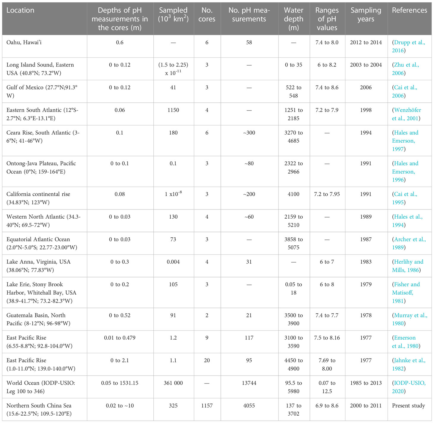
Table 1 Measurements of sediment pH in various published studies.
The sharp decrease in pH in top 2 cm is usually attributed to production of CO2 by aerobic respiration of organic carbon (OC), but secondary oxygenation reactions (oxidation of HS- and Mn2+ by oxygen) may be even more important in the production of H+ (Jourabchi et al., 2005) in the oxic zone. Other important sources of H+ are denitrification, sulfate reduction, oxidation of Fe2+, and precipitation of authigenic MnCO3 and FeS in the suboxic and anoxic zones (Jourabchi et al., 2005). Different geochemical processes may consume H+ in the top 2 cm layer, such as calcite dissolution, Mn(IV) reduction, Fe(III) reduction and sulfide oxidation by MnO2 and Fe(OH)3, but their buffer capacity is weaker than H+ production in this layer (Jourabchi et al., 2005). Below the oxic and suboxic zones is the anoxic zone, where redox activity producing H+ decreases, and diffusion strongly influences vertical pH variations (Jourabchi et al., 2005). However, the latter study only addressed the top meter of the sediment.
According to Einstein’s diffusion equation (Robinson and Stokes, 1970), the vertical variability of pH in the top 10 m of the sediment should be small because of the high diffusion coefficient of hydrogen ions (Li and Gregory, 1974). In this vein, a review chapter (Widdicombe and Spicer, 2011) states that pH profiles “typically follow a sharp decrease from the top sediment layer to a pH minimum situated just below the oxic zone (usually the top few millimeters or centimeters) and subsequently pH becomes invariable with depth”, but this statement was based on a study that had only considered the top 20 cm of the sediment (Burdige et al., 2008). Hence even if sulfate reduction produces H+ and calcite dissolution consumes it in the anoxic zone, pH is not expected to show major variations. However, this hypothesis would need to be tested with field pH data; but very few, if any studies have analyzed vertical pH variability between 1 and ~10 m in the sediment (Table 1).
At the other end of the depth spectrum, the Integrated Ocean Drilling Program collects information on the pH of deep-sea sediment cores (IODP-USIO, 2020). Two pH profiles from the Atlantic Ocean (down to 300 and 600 m in the sediment) show that pH is not invariable below the oxic zone, and low pH values tens of meters down the cores were explained by in situ calcification and AOM (Turchyn and DePaolo, 2011). At the intermediate depth scale of interest to the present work, pH values down to ≥10 m were reported in a study on organic matter diagenesis and mineral processes in sediment cores of the South Atlantic, but the authors did not analyze the vertical pH variations because they used this variable as environmental parameter (Schulz et al., 1994). The word “diagenesis” in the previous sentence refers to physical and chemical changes in sediments after deposition, under the effect of physical, chemical and biological (that is, diagenetic) processes.
In the sediment, porewater is not simply buried along with the settling particles, but its chemical characteristics reflect both the in situ geochemical processes that occur at various depths and the effects of diffusion, advection and bioturbation (Berner, 1980; Jourabchi et al., 2005). Diffusion plays an important role in the transport of dissolved chemical species near the sediment-water interface (Emerson et al., 1982), and can also affect the vertical distribution of properties in porewater much deeper. For example, Adkins et al. (2002) reported that the concentration of chloride in the pore fluid, which is largely unaffected by diagenesis, was sensitive to diffusion in excess of 140 m below the seafloor.
The pH also varies vertically and horizontally depending on the different geochemical processes in different regions. In methane seepage areas, methanogenesis and anaerobic oxidation of methane (AOM) are often associated with sulfate reduction (Miao et al., 2021; Miao et al., 2022). It is thought that in the methanogenesis zone, pH can fall to ~5 (Soetaert et al., 2007; Turchyn and DePaolo, 2011), whereas the AOM generation of two mol-equivalents of alkalinity per mol of dissolved inorganic carbon produced () can lead to an increase in pH in the pore fluid up to ~7.9 (Soetaert et al., 2007; Blouet et al., 2021). Indeed, the associated effect of sulfate reduction on pH switches from consuming H+ at low pH (up to about 6.9) to producing H+ at high pH (Blouet et al., 2021).
Previous studies have investigated the vertical variability of pH at the scale of either centimeters in surface sediment (≤2 m), or tens of meters over several hundred meters (Table 1). Very few studies, if any, have investigated the meter-scale variability of pH between these two depth ranges. The present study does not address the vertical variability of pH in the surface few centimeters of the sediment, which had been the focus of most previous studies on sediment pH. The objectives of the present study are, for the first time in the literature, to describe the spatial and geological time-scale variability of sediment pH in the top ~10 m of the sediment of a deep-sea environment, and propose processes to explain the observed vertical distribution of pH in this sediment. A key objective of the study is to test, down to 10 m in the sediment, the hypothesis found in the literature that diffusion controls the vertical distribution of sediment pH.
Our unique sediment pH dataset comes from 1157 cores collected along the continental slope of the northern South China Sea (nSCS) during 13 oceanographic cruises between years 2000 and 2011. The sediment cores were collected at depths ranging between 137 and 3702 m (Figure 1), their average length was 2.6 m, and the longest core reached 11.9 m.

Figure 1 Study area showing the sampling locations of the 1157 sediment cores along the northern continental shelf of the nSCS. The red dots on the inset map indicate the locations of ODP sites 1144 to 1148 mentioned in the text (IODP-USIO, 2020).
We described the instruments used for core sampling and pH measurements in a previous paper (Shao et al., 2016); see also Supplementary Material 1). Briefly, the cores were taken using a Benthos Piston Gravity Corer or a Benthos Gravity Corer, with a PVC plastic liner placed inside the steel core barrel. When the corer arrived on board the ship, the core in its plastic liner was extracted and quickly cut into several sections, and each section kept in its plastic liner. Measurements of pH and other variables were only done on the sections that presented a good sediment surface.
The pH of the in-core sediment was measured on the head end of each section without extraction of the sediment from the plastic liner or porewater from the sediment. This was done using a method that had been successfully implemented in several studies (Cai, 1992; Cai and Reimers, 1993; Schulz et al., 1994; Cai et al., 2000), and is different from the method recommended by the Integrated Ocean Drilling Program where pH is measured on extracted interstitial water (Expedition 302 Scientists, 2006; Expedition 329 Scientists, 2011). In our study, the sensor was carefully inserted into the center of the head end of the sediment core to a depth of 2-3 cm (that is, the tip of the pH glass sensor reached the depth of 2-3 cm below the upper surface of every section), and the pH value (National Bureau of Standards, NBS, scale) was recorded as the sensor stabilized (that is, within 0.5-1.0 min). Every measurement was performed at least twice, and the mean value calculated. The pH measurements for surface sediment were completed within 10 min of the core arrival on board the ship, and for deeper sediment sections within 5 min after the sections were cut from the core. Overall, pH measurements for all sections of a core were completed within 3 h of the core arrival on board the ship. Details about the sampling, transportation and storage of cores, measurement of pH on cores on board the ship are provided in our previous paper on subsurface-sediment pH (Shao et al., 2016).
The porewater ORP was measured at the same time as pH using a Mettler Toledo FiveEasy™ pH/mV Meter. The temperature of each sediment section was measured at the same time as pH using an instrument that combined a TP-K02 immersion probe CENTER-300 and a thermocouple thermometer, for later temperature correction of pH. At the time of core sampling, in situ bottom-water temperature above the seafloor was measured at some stations using a XXG-T Marine geothermal gradient measurement system (Luo et al., 2007), and seafloor depth was determined with a SeaBeam 2112 Multibeam Bathymetric Sonar. After pH and ORP had been measured on board the ship, each sediment-core section was sealed at both ends, and stored in a refrigerator at 4°C. The concentrations of solid OC and CaCO3 were measured later on sediment samples in a land laboratory following the procedures of the Standardization Administration of the People’s Republic of China (Yan and Huang, 1993; Zhang et al., 1998; Ma et al., 2008; Wang et al., 2010). The measured OC corresponded to total organic carbon.
We summarize here the complementary approaches we used to ensure the quality of pH data. Details of these approaches are provided in Shao et al. (2016) for subsurface-sediment pH, and more details on pH corrections are given in Supplementary Material 2.
The pH of deep-water sediment is sensitive to changes in temperature and pressure that occur when a core is raised from its deep-sea environment to the deck of the ship. In order to minimize temperature effects and avoid exposure of the samples to air, pH was measured in the surface sediment of undisturbed core sections, without extraction. It was explained above that this approach has been successfully used in several previous studies.
We corrected the measured pH for any existing difference between the temperature of in situ bottom water and that of the sediment core at the time of measurement using equations (1) and (2) given in Shao et al. (2016). The accuracy of this correction is not better than about ±0.02 pH unit when the measurement and in situ temperatures differ by 20°C (Gieskes, 1969). To account for the decrease in hydrostatic pressure, we corrected the measured pH values to the in situ hydrostatic pressure using equation (3) in Shao et al. (2016). These two corrections had been applied in previous studies to correct pH in cases where the temperature and/or pressure of measurements differed from those in situ (Culberson and Pytkowicz, 1968; Murray et al., 1980).
It was pointed out by Emerson et al. (1982) that decrease in pressure can cause changes in porewater carbonate system parameters, whose magnitude is variable and related to the carbonate content of the sediment. However, these authors indicated that pH may remain constant as the hydrogen ions released during carbonate precipitation are adsorbed by solid surfaces. If so, the carbonate content of the sediment should not have affected much the pH changes related to pressure decrease during the retrieval of cores. We also explained in Shao et al. (2016) that the so-called “suspension effect” or “colloid effect” in sediment porewater is negligible when pH is measured on marine sediments with a combined glass electrode (Cai, 1992; Cai and Reimers, 1993).
Our data are stated on the NBS pH-scale as previously done by Cai et al. (2000). When salinity varies between 20 and 35, the salinity-related difference between values on the NBS and Seawater pH-scales should range between 0.002 and 0.042 pH unit (Table 7 in Hansson (1973). This difference is much smaller than the vertical variations of >0.1 pH units between two successive sampling depths in most cases in the nSCS and using either pH-scale would not affect our analyses. In addition, vertical variations in salinity are small in nSCS sediment, where they range between 30 and 35 (IODP-USIO (2020). Hence, we did not attempt to correct the NBS pH-scale measurements for salinity in the present study.
Overall, 4055 pH measurements were made on board the ship on different sections of the 1157 cores from the nSCS (Figure 1, Table 2). Because the surface of 4 of the 1157 cores was not appropriate for insertion of the pH sensor (see above), there were only 1153 subsurface-sediment pH data (that is, shallower than or at 0.05 m). Deep-sediment pH (that is, 0.05 m to bottom) was measured on 968 of the 1157 cores, and a total of 2902 values were determined on the non-surface sections of the cores. Hence, there were both subsurface- and deep-sediment pH measurements on 968 of 1157 cores. The total number of pH data available for the present study was thus 1153 + 2902 = 4055.
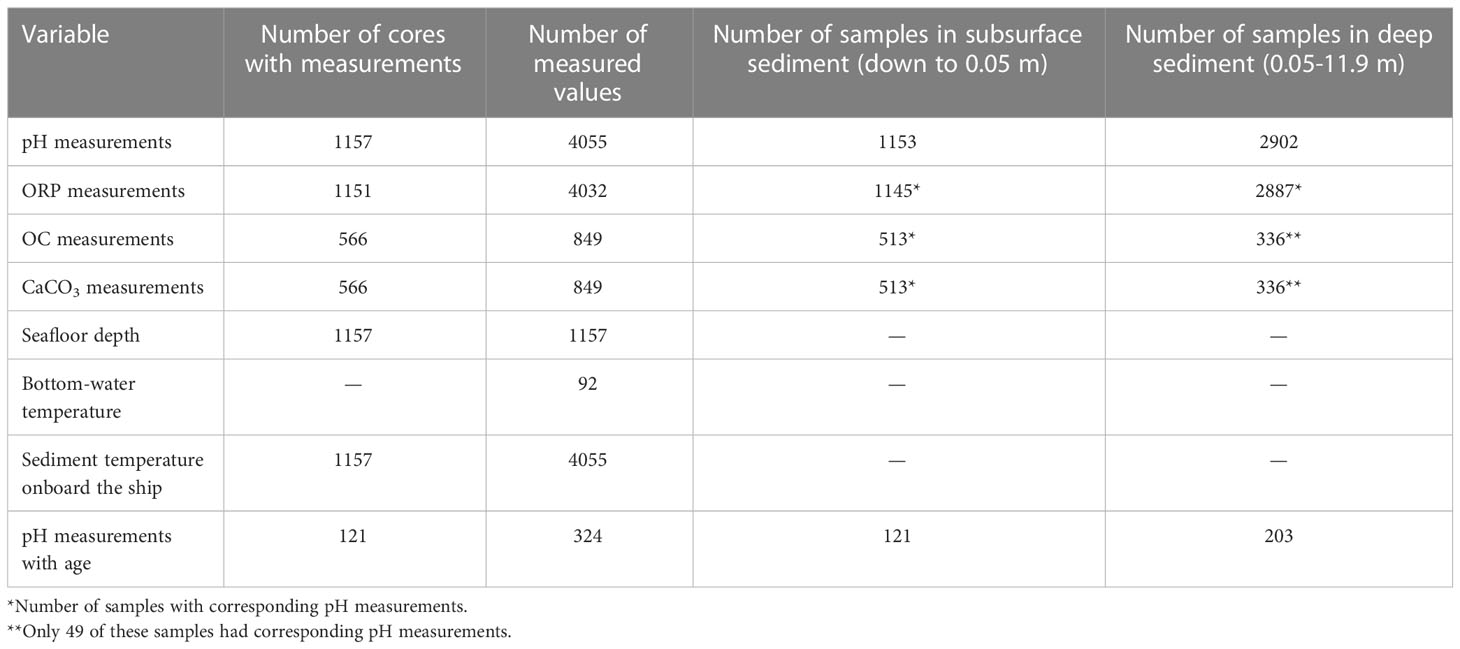
Table 2 General information on the dataset.
There were 4032 measurements of sediment ORP on different sections of 1151 cores, that is, 1145 and 2887 subsurface- and deep-sediment ORP, respectively. The concentrations of solid OC and CaCO3 were determined on the solid sediment of 849 samples from 566 cores, that is, 513 and 336 subsurface- and deep-sediment concentrations, respectively. The number of cores with measurements of pH and ORP and concentrations of OC and CaCO3 was 513, and the number of cores with deep-sediment measurements of the four variables was 49. No additional chemicals were measured in porewater or on solid sediment.
During the cruises, seafloor depth was determined at the 1157 coring sites, and in situ bottom-water temperature was measured at 92 stations. In addition, temperature was measured on board the ship on the 4055 core sections.
In order to investigate the mechanisms influencing the spatial variations in pH, we separated our pH data in the two depth groups defined above, that is, subsurface (≤0.05 m) and deep (>0.05 m) with 1153 and 2902 values, respectively. We assumed that samples in the first group experienced intensive redox processes and were the mass-exchange gateway between seawater and the surface sediment, and those in the second group were subjected to weaker redox processes (Jourabchi et al., 2005; Burdige, 2006). In the text below, we sometimes compare the values in subsurface sediment with those from intermediate (0.05 to 2.0 m) and bottom (2.0 to ~10 m) sediment (we chose the depth of 2.0 m for the practical reason that the length of most cores was at least 2.0 m). It should be remembered that our study does not address the detailed vertical distribution of pH in the upper millimeters or centimeters of the sediment, and thus has no data comparable to the surface-sediment pH values measured or modeled in studies devoted to millimetric or centimetric scales.
To analyze the relationships between subsurface- and deep-sediment pH, we used the division of our study area into the four regions that we had defined in our previous study, where we had investigated the relationships between subsurface-sediment pH and the characteristics of the overlying water column in the nSCS (Shao et al., 2016). These regions were based on the subsurface-sediment contour line pH = 7.5 of (Figure 2A), which delineated areas with pH lower and higher than 7.5. The regions are, from west to east: H (south of Hainan Island), P (Pearl River plume and a downstream submarine canyon), K (area influenced by the western branch of the Kuroshio Intrusion Current) and T (southwest of the coast of Taiwan Island) (Figure 2A). To illustrate the horizontal distribution of intermediate-sediment pH, we projected the vertical pH values between 0.5 and 2 m onto a horizontal plane (Figure 2B).
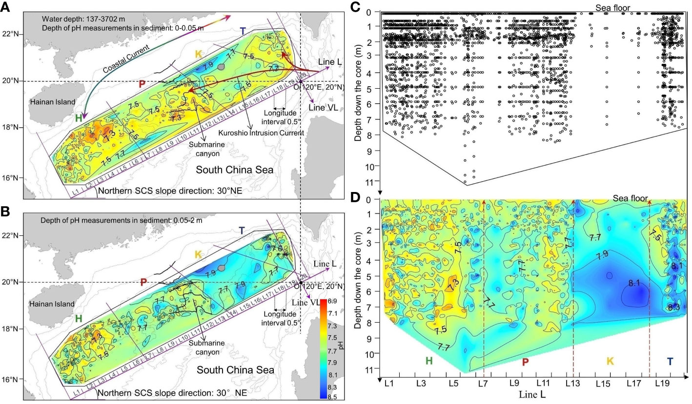
Figure 2 Interpolated maps of sediment pH in the nSCS sediment. Spatial distributions of pH were obtained by natural neighbor interpolation based on (A) 1153 discrete subsurface samples, and (B) 1493 discrete intermediate samples (all values were projected onto a single horizontal plane); line L is oriented 30° to the NE, corresponding to the general direction of the continental slope, and goes through point O. (C) Positions of the 4055 pH data from all depths projected onto a single vertical plane along the continental slope on line L, and (D) depth distribution of pH along line L. The four regions are based on the contour line of subsurface-sediment pH = 7.5: south of Hainan Island (H), Pearl River plume and connected submarine canyon (P), area influenced by the western branch of the Kuroshio Intrusion Current (K), and southwest of the coast of Taiwan Island (T) (Shao et al., 2016).
We represented the vertical pH variations (Figures 2C, D) by projecting all available pH values onto a 2-D vertical plane parallel to the continental slope, that is, line L shown in Figures 2A, B. Line L is oriented 30° to the NE, which corresponds to the general direction of the continental slope in the nSCS, and goes through point O (120°E, 20°N). Line L is defined by the following equation:
Where A=−tan30° , B=1 , and . Based on equation (1), we calculated the geographic position of each in situ point M(xin·situ,yin·situ) projected on line L, N(xprj,yprj) , as follows:
The depth of each point in the projected plane was the same as its in situ depth.
To obtain continuous pH values (Figure 2), we subjected all discrete data points in the horizontal or vertical projection planes, including the data points from a same station, to natural neighbor interpolation as explained in Shao et al. (2016). We used the ArcMap software for the calculations.
The 968 cores with at least 2 pH measurements on the vertical were grouped using the following clustering technique. Given that the pH values had been measured at different depths on different cores, we performed interpolation to obtain evenly distributed data with depth in the cores. We used a linear model for simplicity. To do so, we first fitted the following equation to each vertical pH profile, where pH (y ) was a function of sediment depth (x ):
and used equation (3) to calculate the values of pH at 10 cm intervals along the core, starting at 0 cm (surface of the core), where k was the regression (slope) coefficient and b was the intercept (constant) value. We used equation (3) to interpolate pH values on the vertical assuming linear distribution of pH values as a function of sediment depth between successive sampling points.
Using the pH values at 10 cm intervals, we then clustered the vertical pH profiles as follows. First, we computed the Euclidean distance between each pair of profiles. Second, we clustered all pairs of profiles with the smallest Euclidean distances. Third, we computed the median profile for each of the cluster. Fourth, we added to one of the clusters the pH vertical profile with the smallest Euclidean distance, and repeated the operation until all profiles had been included in one of four clusters, identified below as core clusters 1, 2, 3 and 4. Fifth, we determined the median pH value in each cluster at each 10 cm depth.
We found in the literature 18 cores with age information located in our nSCS study area (Supplementary Material Table S1). To transfer the age information from the 18 dated cores to our sampled cores with pH data, we first selected all cores located in a circle with a radius of 0.5° longitude around each of the 18 dated cores, and considered that all sampled cores within that circle had the same age as the reference dated core. There were 121 of our cores with pH determinations located within 0.5° longitude of the 18 dated cores. We then used linear interpolation (for simplicity) to calculate, for each of the 121 cores, the age of the sediment (yage) at each depth with a pH measurement (xdepth):
where xlower and xupper were the lower and upper values, respectively, of the depth interval containing xdepth in the reference core, and ylower and yupper were the ages of the sediment at xdepth in that core. This way, we ascribed a sediment age to each of the 324 pH data in the 121 cores. Out of the 121 cores, 93 had ≥ 2 pH data.
In order to analyze the variability of pH down the cores, we transformed the vertical changes in pH into absolute changes in hydrogen ion concentration [H+], because changes in pH reflect relative changes in [H+], not absolute changes (Fassbender et al., 2021). To do so, we combined equations 3-5 of Fassbender et al. (2021) to calculate Δ[H+] as follows:
where [H+]upper , [H+]deeper , pHupper and pHdeeper are the [H+] and pH values measured at two consecutive depths down the core, respectively, and the units of Δ[H+] are mol L-1.
We quantified the variability of [H+] and other variables down the cores by calculating for each core the differences between successive values from the sediment subsurface downwards. The formula for [H+] was as follows:
where the units of Δ[H+]depth are mol L-1 m-1. We did the same calculations for ΔORPdepth, ΔCaCO3 depth and ΔOCdepth (units: mV m-1, CaCO3 concentration m-1, and OC concentration m–1, respectively).
Similarly, we calculated sediment age differences between successive [H+] values down cores (mol L–1 ka–1) as follows:
where pHold and pHyoung are the pH values corresponding to two successive sediment ages down the core, and the units of Δ[H+]age are mol L–1 ka-1. We did the same calculations for ΔORPage (units: mV ka–1).
In order to find patterns in vertical [H+] profiles, we first normalized each [H+] value down each core to [H+]subsurface as follows:
Where [H+]subsurface , [H+]depth , pHsubsurface and pHdepth are the [H+] and pH values at each sampling depth below the subsurface of the core and at the subsurface, respectively. We made this calculation for all sampling depths along each core. The resulting [H+]* profiles could be systematically compared because their subsurface values were the same, that is, [H+]∗subsurface=0. In other words, the vertical [H+]* profiles were independent of their subsurface-sediment [H+] values.
We then grouped the vertical [H+]* profiles as follows. First, we selected the [H+]* profiles where all the values -0.1x10⁻⁸ mol L-1 m-1< [H+]*< 0.1x10⁻⁸ mol L-1 m-1. We considered that the values of these profiles (group a) were uniform with depth in the sediment, and removed these profiles from the next steps. Second, we selected the [H+]* profiles with more positive than negative values (group b) as showing a general increase in [H+] (or decrease in pH) with depth. Third, we selected the [H+]* profiles with more negative than positive values (group c) as showing a general decrease in [H+] (or increase in pH) with depth. Fourth, we assigned the [H+]* profiles with an equal number of positive and negative values to either group b’ or c’ (defined in the same way as groups b and c) after removing their [H+]* value closest to 0, based on the idea that this value had the highest likelihood of being randomly positive or negative.
We described the vertical variability of pH and [H+]* with depth by computing median values at successive depths. We used equation (3) to calculate the values of pH at 10 cm intervals along the core, and used the results to compute the median values.
We used contingency table analysis to determine the relationship between the division of cores into four regions and their grouping into four clusters. We also used this analysis to determine the relationships between the three types of vertical [H+]* profiles (uniform, positive, and negative) and environmental variables. In order to do so, we first entered in each cell of contingency table the observed number of cores (O) in the given region and cluster, or the given [H+]* profile type and category of the environmental characteristic under consideration. We then computed for each cell the expected values (E) under the hypothesis of independence between the two variables:
We finally computed the Wilks’ G2 and its associated chi-square probability to test the hypothesis of independence (H0) between the two variables. In contingency tables, we considered cells with (O-E)/[(O+E)/2] >0.3 and<0.3 as indicative of positive and negative correspondence, respectively.
Overall, the pH values ranged between 6.9 and 8.6, the highest value occurring at 4 m in a core of region T (Figure 3). and there were large horizontal variations in the pH of subsurface and intermediate sediment (Figures 2A, B). Median pH values in the four regions generally increased eastwards in both subsurface and intermediate sediment, the highest values being in region K (Table 3). There were corresponding areas of low or high pH values in subsurface and deep sediments, the values in these “chimneys” being vertically coherent from surface down to 8 m (Figure 2D).
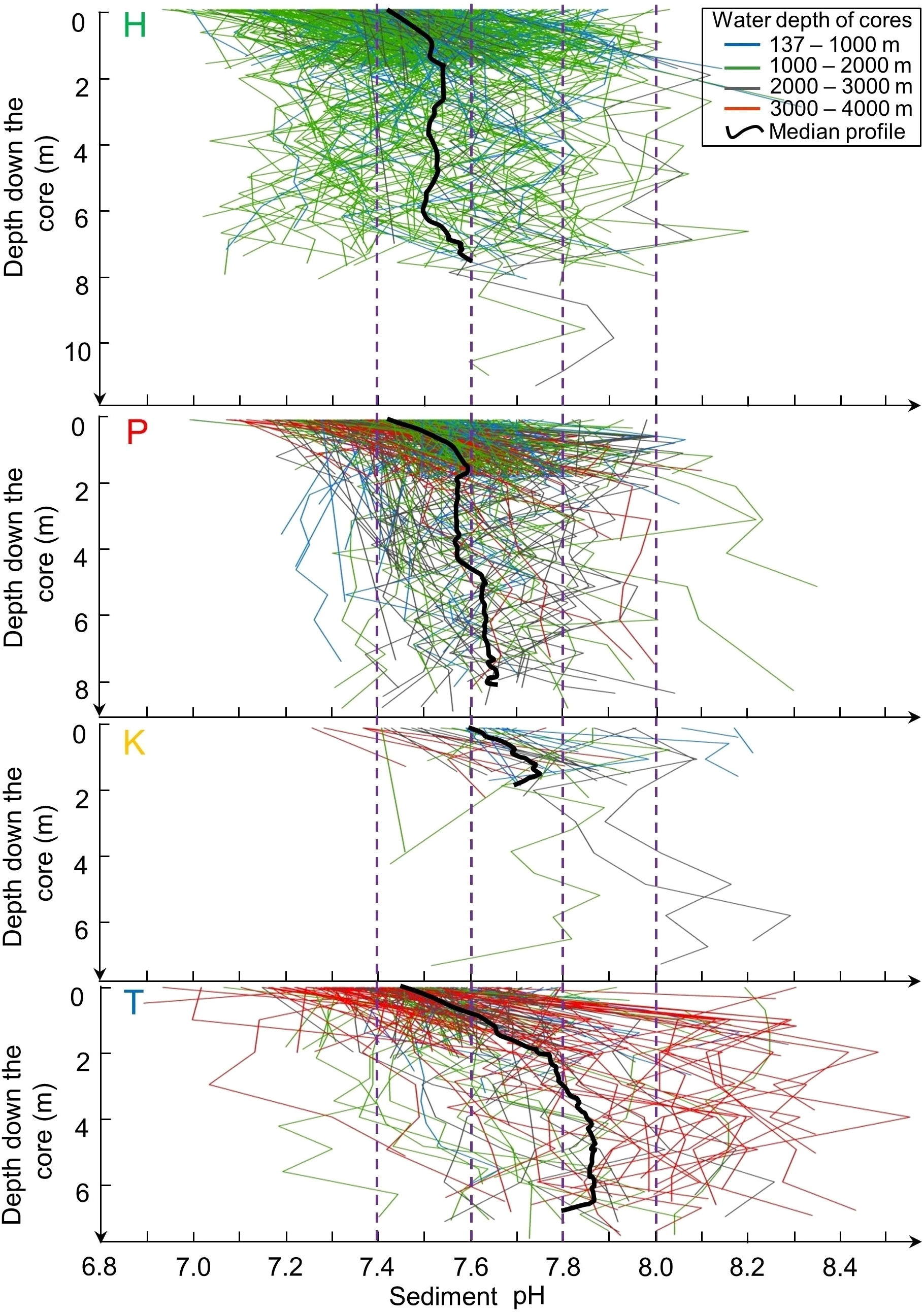
Figure 3 Vertical profiles of pH along the cores as a function of depth in the sediment in the four regions H, P, K and T identified in Figure 2. Black lines: profiles of median values.
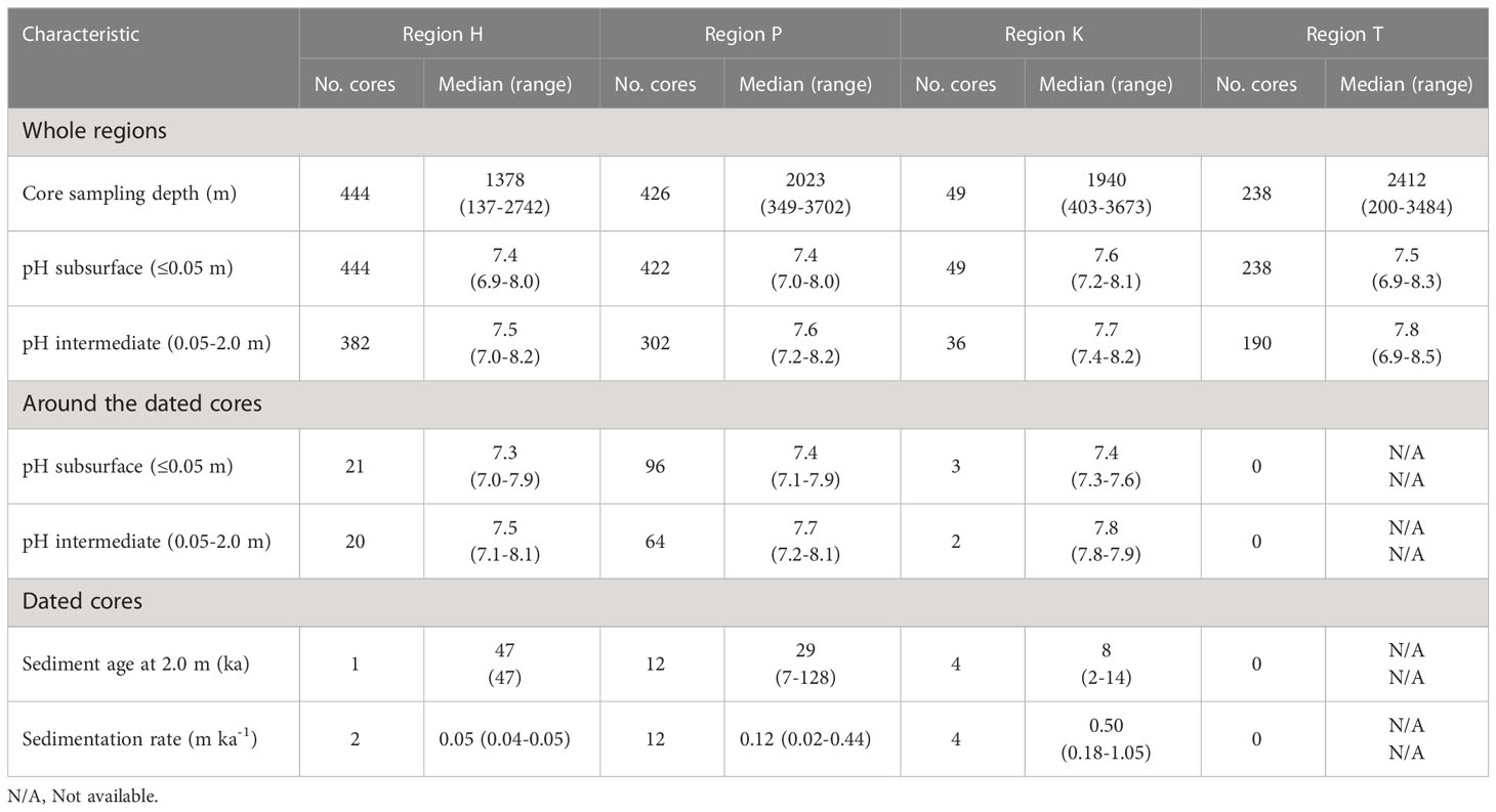
Table 3 Key characteristics of cores (pH, sediment age, and sedimentation rate) in the four regions of the nSCS.
The pH of subsurface sediment was lower than that of intermediate sediment in the whole nSCS (mean values of 7.4 and 7.6, respectively; unpaired t-test, p< 0.001) and also in each of the four regions (Table 3). Below the sediment subsurface, pH in the four regions showed a generally increasing trend with depth in the upper 2 m, and less variability below (Figure 3). This was also the case in the core clusters obtained by free clustering of sediment cores based on their vertical pH profiles (Figure 4; Table 4). Cluster 4 grouped together only four sediment cores (corresponding to the rare pattern of decreasing pH with increasing sediment depth; yellow asterisks in Figure 4A), and was thus not considered in subsequent calculations and discussion.
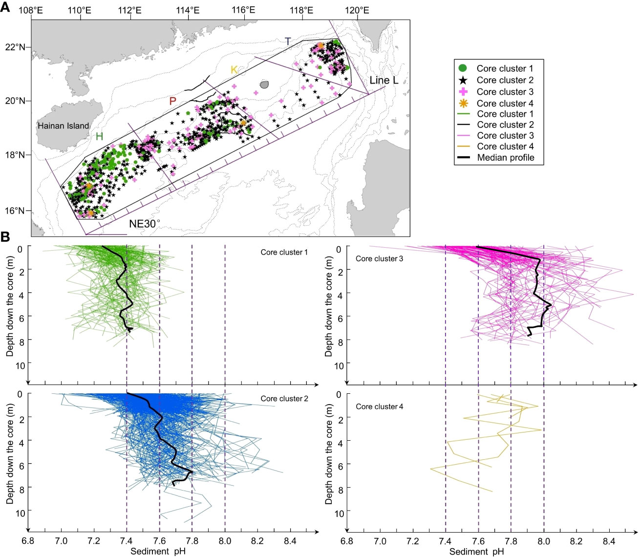
Figure 4 Clusters of sediment cores based on the vertical distributions of pH along the cores. (A) Spatial distribution of the four clusters. (B) Vertical profiles (0 to ~10 m) of pH as a function of depth in the sediment cores of the four clusters. Black lines: profiles of median values (except cluster 4 where there were only four profiles).
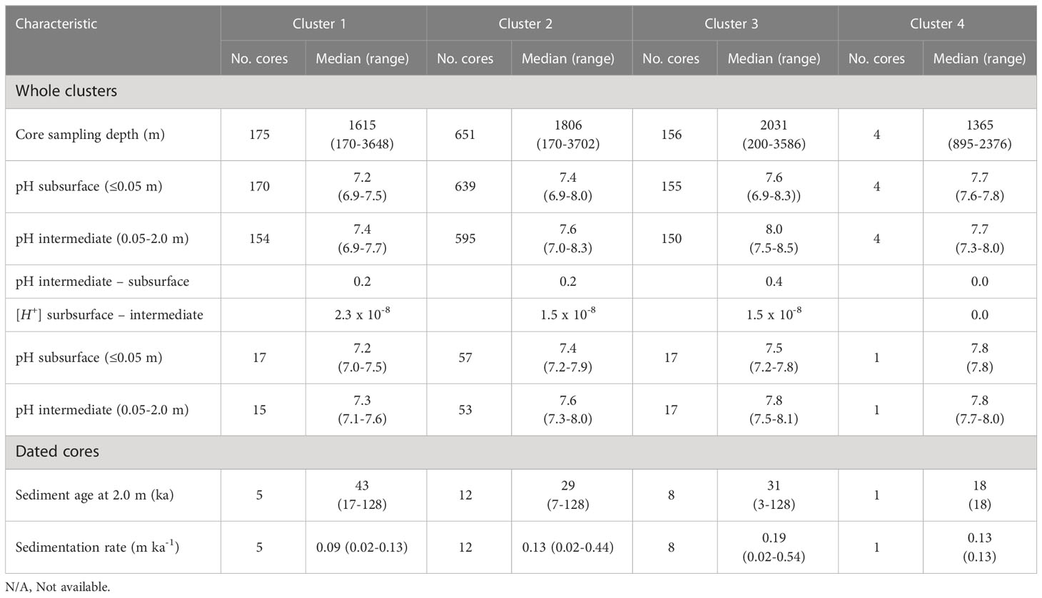
Table 4 Key characteristics of cores (pH, sediment age, and sedimentation rate) in the four core clusters of the nSCS.
There was an overall correspondence between the horizontal pattern of suburface pH and the vertical distributions of pH in the deep sediment (contingency table analysis: p< 0.0001; Supplementary Material Table S2). The contingency table shows that cluster 1, whose pH varied on the vertical around 7.4 was especially well represented in the western part of the nSCS (region H), and cluster 3 (pH ~8.0) in the eastern part (regions K and T) (Supplementary Material Table S2).
We calculated the change in [H+] per unit depth (Δ[H+]depth ) for each successive pair of pH measurements down each of the 968 cores with at least 2 pH data (Figure 5A). Positive and negative Δ[H+]depth indicate increasing and decreasing [H+] with depth, respectively. The numbers of positive and negative Δ[H+]depth values at different depths show that [H+] decreased rapidly with increasing depth in the upper 2 m (that is, larger numbers of negative than positive values), and was less variable below (Figure 5B).
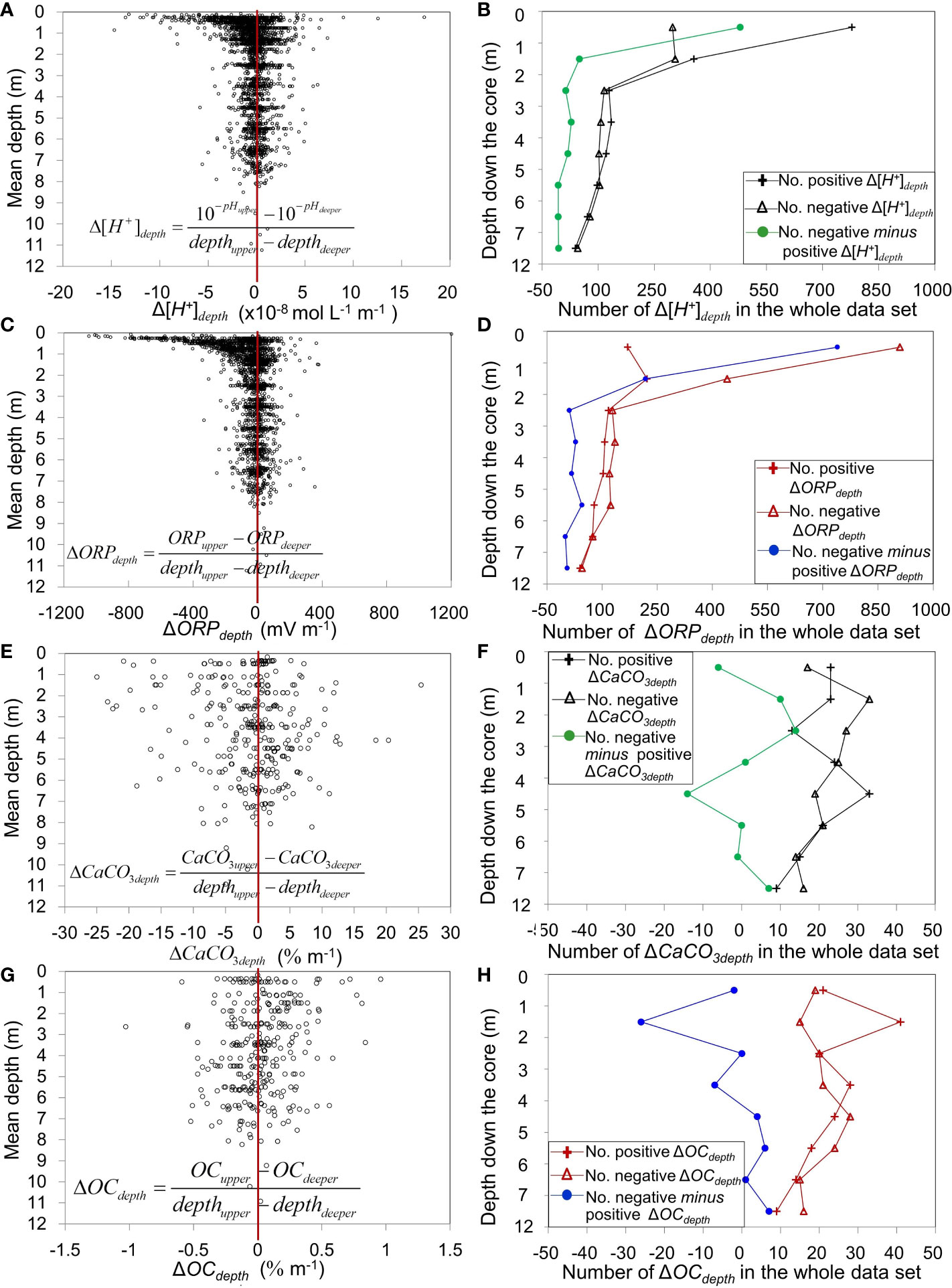
Figure 5 Depth distributions of the differences between two consecutive values down the cores for the whole dataset. Depth differences and distributions of positive and negative values in (A, B) Δ[H+]depth, (C, D) ΔORPdepth (5 values > 1000 are not shown), (E, F) ΔCaCO3depth, and (G, H) ΔOCdepth (Supplementary Material Tables S3, S4). Positive (negative) Δ[H+]depth, ΔORPdepth, ΔCaCO3depth and ΔOCdepth: increasing (decreasing) values with increasing depth. For Δ[H+]depth and ΔORPdepth, there were 2884 paired values from 968 cores, that is, total of 1157 cores with pH and 1151 cores with ORP measurements, among which there were 968 cores with at least 2 values for both pH and ORP measurements. For ΔCaCO3depth and ΔOCdepth , there were 333 paired values from 46 cores, that is, total of 49 cores with CaCO3 and OC measurements, among which there were 46 cores with at least 2 values for both CaCO3 and OC measurements.
We had data for three variables that have important roles in diagenetic geochemical processes in marine sediments. These were the ORP measured on porewater at the same time as pH, and the concentrations of CaCO3 and OC in solid sediment. Similar to [H+], the ORP decreased with increasing depth in the upper 2 m and was more constant below (Figures 5C, D). Concentrations of CaCO3 and OC in the sediment did not exhibit coherent patterns of vertical variability between the subsurface and 8 m (Figures 5E–H).
Patterns in standardized vertical [H+]* profiles were as follows (Figure 6). Overall, median [H+]* values below the subsurface were negative, indicating generally lower [H+] at depth than 2-3 cm below the sediment surface (Figure 6A). Among the 968 [H+]* profiles, 2.2% (28 profiles) were uniform with depth -0.1x10⁻⁸ mol L-1 m-1< [H+]*< 0.1x10⁻⁸ mol L-1 m-1; Figure 6B), 80.3% had mostly negative values (777 negative profiles, of which 729 and 48 belonged to groups c and c’, respectively; Figure 6D), and 17.5% had mostly positive values (170 positive profiles, of which 170 and 0 belonged to groups b and b’, respectively; Figure 6C).
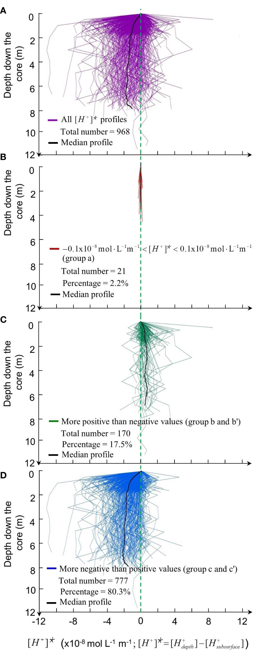
Figure 6 Vertical profiles of [H+]* along the cores as a function of depth in the sediment. (A) Total 968 [H+]* profiles. (B) 21 uniform profiles with -0.1x10‑8 mol L‑1 m-1 < [H+]* < 0.1x10⁻⁸ mol L‑1 m‑1 (group a). (C) 170 mostly negative values (group b and b’). (D) 777 mostly positive [H+]* values (group c and c’). Black lines: profiles of median values.
Among the 18 cores with sediment age information we found in the literature, those located within 40 km of each other had similar depth distributions of ages, and thus similar sedimentation rates. Examples of such pairs of cores and their sedimentation rates are: MD97-2146 and ODP17940 (1.05 and 0.54 m/ka), ODP1145 and ODP17937 (0.23 and 0.18 m/ka), and V36-06-5 and V36-07 (0.13 and 0.10 m/ka) (Figure 7; Supplementary Material Table S1). We thus confidently paired the sediment ages of these 18 cores with the data of our 121 sampled cores located in their vicinities (Figure 7). Out of these 121 cores, 93 had at least 2 pH measurements.
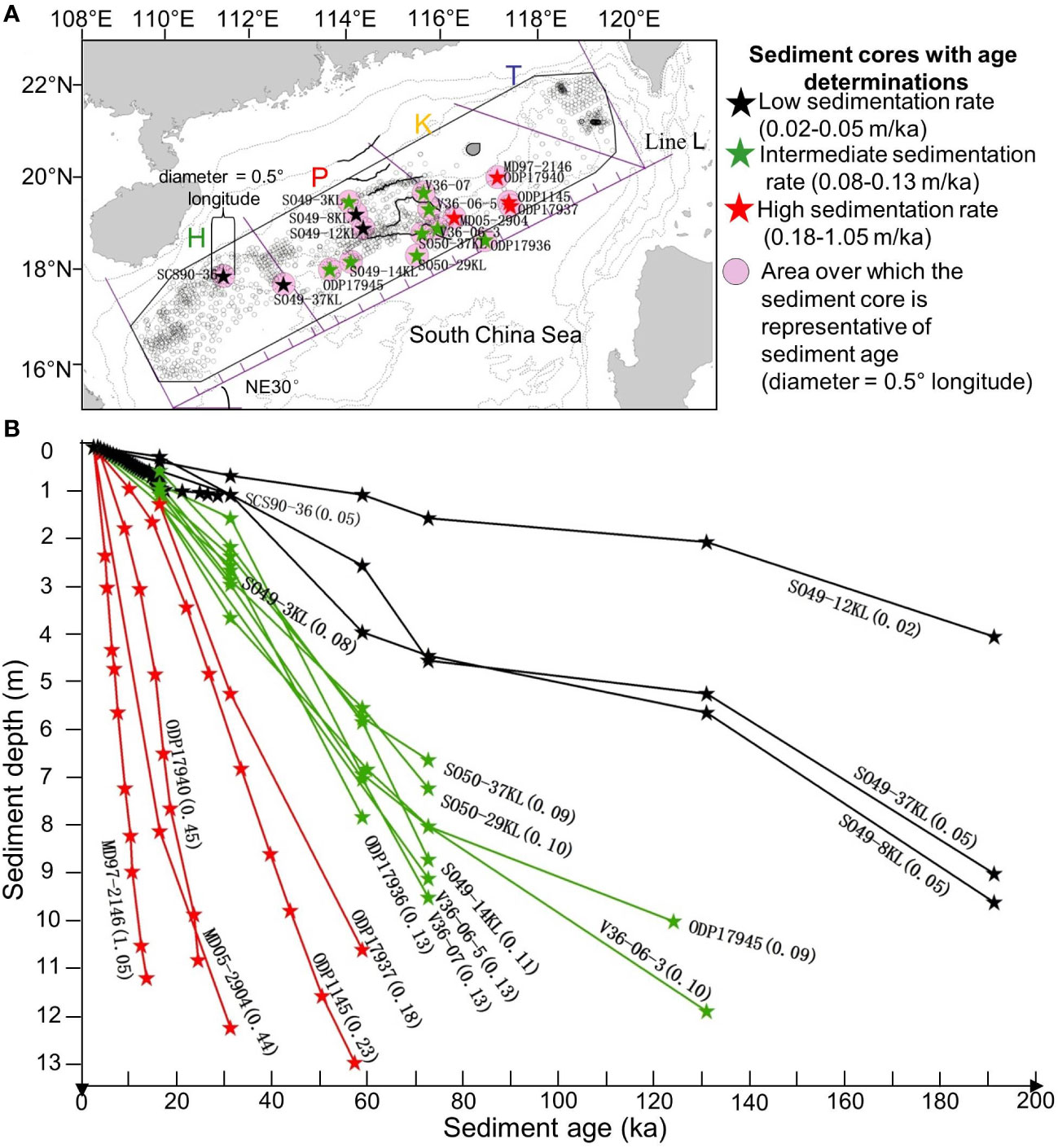
Figure 7 Sediment ages in the nSCS. (A) Locations of 18 cores (from the literature) with sediment age determinations (Supplementary Material Table S1). A total of 121 of our cores were located in the pink circular areas around the 18 cores (diameter = 0.5° longitude); we considered that the ages of sediments in these cores where the same as those of the reference core. (B) For the 18 cores in panel (A), variation of age as a function of depth in the sediment. Near the end of each profile: same core code number as in panel (A), and sedimentation rate (m ka-1) computed from the linear regression (Model I) of all age values on corresponding depths in each profile. The sediment ages along these cores were paired with 324 pH determinations made along our 121 cores (values used in Figure 8).
We calculated the change in [H+] per unit sediment age (Δ[H+]age ) for each successive pair of pH measurements down each of the above 93 cores (Figure 8A). Positive and negative Δ[H+]age indicate increasing and decreasing [H+] with sediment age, respectively. The resulting values show that [H+] decreased with increasing sediment age from present back to 20-40 ka, and were relatively constant in older sediment back to 160 ka (Figure 8B). Similar to [H+], the ORP decreased with increasing sediment age from present back to 20-40 ka, and was more constant back to 160 ka (Figures 8C, D).
Linear regressions of pH on ORP values show that, for the whole sampling area, subsurface-, deep- and total-sediment pH were significantly related to the ORP values (Supplementary Material Figure S1). In addition, the average ORP values were higher in subsurface- than deep-sediment (t-test, p< 0.001).
The results of contingency table analyses of the three types of [H+]* profiles (uniform, positive, and negative) with environmental characteristics were as follows. There were strong relationships with water depth (p< 0.0001; Supplementary Material Table S6), seafloor temperature (p< 0.0001; Supplementary Material Table S7) and subsurface sediment pH (p< 0.0001; Supplementary Material Table S8), a weaker relationship with the solid OC content (p = 0.02; Supplementary Material Table S9), and no relationship with the solid CaCO3 content (p = 0.35; Supplementary Material Table S10). The contingency tables show that there were more observed positive profiles than expected (O > E) in shallow waters, at high seafloor temperatures, and corresponding to high subsurface pH and high solid OC. Conversely, there were less observed positive profiles than expected (O< E) in deep waters, at low seafloor temperatures, and corresponding to low subsurface sediment pH and low solid OC; also, there were less observed negative profiles than expected (O< E) corresponding to high subsurface pH (Supplementary Material Tables S6–S10).
The time scale for the vertical diffusion of a solute signal from ocean-bottom water or surface sediment down to 12 m in the sediment can be calculated using Einstein’s diffusion equation (Robinson and Stokes, 1970):
where T is the average time required to diffuse at distance L, L is depth in the sediment, and DH+ is the hydrogen ion diffusion coefficient. In our case, L = 12 m = 1200 cm.
The diffusion coefficients of ions in deep-sea sediment (Dj.sed.) is related to the seawater diffusion coefficient () as follows (Ullman and Aller, 1982):
where ϕ is porosity, and F is the formation resistivity factor which measures the influence of pore structure on the resistance of sample. In order to obtain Dj.sed., we first estimated , ϕ , and F . The value of in seawater is 56 x 10-6 cm2 s–1 (Li and Gregory, 1974). The value of ϕ in marine sediment is predicted to be 0.4-0.9 (Martin et al., 2015). Finally, F is empirically related to ϕ as follows (Ullman and Aller, 1982):
where m=2 for ϕ=0.2−0.7 and m=3 for ϕ≥0.7 in deeply buried sediment. We calculated the diffusion coefficient of hydrogen ions in sediment (DH+.sed.) combining equations (11) and (12) and using the above range of values of ϕ and m:
We used this DH+.sed. value, to compute T with equation (10):
The value of T in equation (14) indicates that the average time required for H+ to diffuse vertically over 12 m in marine sediment ranges between 495 and 1020 years. This range of years corresponds to sediment thickness of 0.01-1.07 m in the nSCS (Figure B), meaning that the vertical distributions of [H+] and pH there should be quite uniform down to 12 m in the sediment if solely controlled by diffusion.
Most field, laboratory and model studies on the vertical variability of sediment pH in the literature have focused on changes in the top few millimeters or centimeters of the sediment (Table 1). These studies found that pH generally decreased in the top 5 cm of the sediment (Figure 7 of Shao et al. (2016), as a consequence of OC redox processes (for example, Boudreau, 1997; Jourabchi et al., 2005). Indeed, OC redox processes are the most important sources of [H+] in top sediment (Hales and Emerson, 1996; Reimers et al., 1996; Jourabchi et al., 2005), where the oxidation of OC primarily uses dissolved molecular oxygen (Emerson and Bender, 1981; Reimers et al., 1996). Beneath the oxygen-containing sediment layer, anaerobic bacteria oxidize OC by denitrification, Mn-oxide reduction, Fe-oxide reduction, reducing sulfate to sulfide, and methanogenesis (Ben-Yaakov, 1973; Nealson, 1997; Jourabchi et al., 2005).
Contrary to the above, usual studies, our dataset did not include values from the top few millimeters of the sediment, and had 1153 pH measurements made 2-3 cm below the sediment surface which represented 28% of our 4055 total pH data. Our subsurface values were generally quite low, mostly<8.0 (Figure 2A; Table 3), and were likely representative of the subsurface pH minimum reported in previous studies. The horizontal distribution of subsurface-sediment pH in the nSCS, illustrated in the four regions of Figure 2A, reflected the combined effects of several environmental variables discussed by Shao et al. (2016).
Our present work is different from most previous studies as it explores the top ~10 m of the sediment, which is more than 100 to 200 times deeper than the usual top 5 to 10 cm studied in the literature. In fact, 2902 out of our 4055 pH data (72%) were measured deeper than 5 cm in the sediment. Overall in the nSCS, pH was generally higher in the intermediate sediment down to 2 m than in the above subsurface sediment, and often tended to increase with increasing depth below 2 m (Figures 2B, D). There was much variability among the vertical pH profiles in the four regions (Figure 3), but despite this variability, the vertical distributions of median pH values in the four regions showed a general trend of increasing values with depth in the upper 2 m and underlying values increasing (regions P and T) or being quite vertically uniform (region H). The vertical distributions of median pH values resulting from the free clustering of sediment cores (Figure 4) showed the same general trend as in the four regions, that is, vertically increasing pH in the upper 2 m (clusters 1-3) and underlying values either increasing (cluster 2) or being quite vertically uniform (clusters 1 and 3). This vertical pattern occurred irrespective of the magnitude of pH values, which generally increased from regions H to K-T and clusters 1 to 3 (Figures 3, 4; Tables 3, 4).
The Δ[H+]depth values characterized vertical changes in [H+] between successive depths down the cores, that is, positive and negative values corresponded to vertically increasing and decreasing [H+] with increasing depth, respectively (Figure 5A). Considering all nSCS cores together, the vertical distribution of Δ[H+]depth showed high variability among cores in the upper 2 m and less variability below, indicating that values below 2 m were more vertically uniform values than above 2 m. The same general trend of decreasing [H+] with depth in the upper 2 m and more uniform values below was indicated by the decreasing excess of positive over negative Δ[H+]depth values with depth down to 2 m, and almost equal numbers of negative and positive values below 2 m (Figure 5B).
The strong downward decrease in [H+] in the upper 2 m likely reflected the combined action of a number of diagenetic processes in that sediment layer, including redox reactions, ion diffusion, mineral dissolution, precipitation and authigenic processes (for example, carbonate dissolution/precipitation) (Berner, 1980; Parkes et al., 1990; Cragg et al., 1999). The pattern of vertical changes in ORP (ΔORPdepth ) (Figures 5C, D) was similar to that of Δ[H+]depth (Figures 5A, B). Different from the vertical variability in Δ[H+]depth and ΔORPdepth , the concentrations of CaCO3 in the solid sediment (ΔCaCO3depth) were quite uniform with depth (Figure 5E). The latter may indicate that carbonate dissolution/precipitation was quite uniform in the solid sediment down to ≥10 m, contrary to porewater whose upper 2 m were marked by strong gradients in pH and ORP indicating active diagenesis. The increasing number of negative minus positive ΔOCdepth values with increasing depth (from -26 at 1-2 m to +7 at 7-12 m, Figure 5H and Supplementary Material Table S4) reflected the decreasing number of positive ΔOCdepth values especially below 4 m. Hence as depth in the sediment increased, the number of cores where the solid OC content increased with depth became progressively smaller than number of cores where the solid OC content decreased with depth, which could indicate that redox activity progressively consumed OC as depth in the sediment increased.
Given that sediment diagenetic processes occur at geological timescale, [H+] values in deep sediment reflect geochemical and physical processes that took place over long time scales. We used sediment age to characterize these time scales. The Δ[H+]age and ΔORPage values characterized vertical changes in [H+] and ORP between successive ages down the cores, that is, positive and negative values corresponded to vertically increasing and decreasing [H+] and ORP with increasing sediment age, respectively (Figure 8). The vertical distributions indicated a general decrease in [H+] and ORP with increasing sediment age from present back to 20-40 ka, and relatively uniform values in older sediment, showing that geochemical activity mostly took place during the first 20-40 ka after sedimentation. Combining this with the above depth results indicate that, over the last 200 ka, rapid changes in [H+] (and thus pH) and ORP occurred during the first 20-40 ka, which generally corresponded to the upper 2-m layer of the sediment. In older (>20-40 ka), bottom (>2 m) sediment, the [H+] and ORP characteristics were more vertically uniform. The first 20-40 ka, upper 2-m layer of the sediment was thus the geochemically active period and layer.
In 14 of the dated cores (Supplementary Material Table S1) the depths corresponded to boundaries of Marine Isotope Stages (MIS). We transformed the MIS information into ages using the MIS taxonomy of Lisiecki and Raymo (2005), where the age uncertainty is 4 ka from 1 to 0 Ma. All age values are estimates as they were interpolated using equation (4). In the present study, the determination of the period of the geochemical active layer, i.e. 20-40 ka was not affected by this relatively small uncertainty or by the small errors on the ages of the other dated cores.
The vertical [H+]* profiles provide information on deep-sediment [H+] independent of subsurface-sediment [H+] (and thus pH) values (Figure 6). In the nSCS, 2.2% of the 968 vertical profiles of standardized [H+] (that is, [H+]*) had a uniform distribution with depth (group a, Figure 6B). It was shown in the Results that the timescale for the diffusion of a solute signal down to 12 m in sediment was 495-1020 years, and this timescale corresponded to sediment thickness ≤ 1.1 m in the nSCS. Hence, in 2.2% of the cores where the vertical distribution of [H+] (and thus pH) was quite uniform in the nSCS sediment, the vertical distribution of H+ ions in porewater was dominated by vertical diffusion. Although we do not have information on [H+] production, consumption and flux in our cores, the very small fraction of cores with vertically uniform sediment pH leads to reject, for nSCS sediment down to ~10 m, the hypothesis from the literature that diffusion controlled the vertical distribution of pH in porewater below the subsurface.
In 97.8% of the cores, vertical [H+] profiles were not uniform (Figures 6C, D), and thus not dominated by vertical diffusion. In these cores, combined geochemical processes of production and consumption of H+ ions in porewater (for which we have no data) likely affected [H+] more than vertical diffusion. In the remainder of this section, we examine successively the profiles of decreasing and increasing [H+]* with depth.
Most of the nSCS [H+]* profiles were negative (80.3%, groups c and c’; Figure 6D), that is, [H+] along these cores was generally lower (and thus pH generally higher) than at the sediment subsurface. Two successive mechanisms likely explained net consumption of H+ ions at depth in the sediment over most of the nSCS. First in the top centimeters of the sediment, there is strong consumption of degradable organic matter, and the accompanying release of CO2 causes a decrease in pH. Second below the thin oxic zone, various diagenetic geochemical processes, such as the reduction of iron and manganese oxides and the dissolution of calcite consume H+ ions, thus causing lower [H+] (and higher pH) beneath subsurface sediment. These two points are an extension down to ~10 m of mechanisms described by Jourabchi et al. (2005) for the top 50 cm of the sediment.
The fact that most of the nSCS [H+]* profiles were negative is consistent with the inverse relation between pH and ORP in both subsurface and deep sediment (Supplementary Material Figure S1), which indicated that low pH (high [H+]) generally occurred in porewater with strong oxidation potential. In addition, ORP values >200 mV were more frequent in subsurface than deep sediment (Supplementary Material Figures S1B, C), and the stronger ORP in subsurface porewater could have been caused by high content of electron acceptors (for example, oxygen, nitrate, manganese) (Hunting and Kampfraath, 2013), which would have also led to lower subsurface pH (Jourabchi et al., 2005; Shao et al., 2016), hence the inverse relationships between ORP and pH.
The ORP may have been strongly influenced by bacterial activity (Zobell, 1939; Jourabchi et al., 2005; Hunting and Kampfraath, 2013). Indeed, ORP values in the nSCS were strongly positive in subsurface sediment (>200 mV; Supplementary Figure S1B), where bacteria are generally most abundant (Jourabchi et al., 2005), and most values were<200 mV below the subsurface sediment (Supplementary Figure S1C), where total bacterial numbers and the frequency of dividing cells are reported to decrease rapidly (Zobell, 1939; Parkes et al., 1990; Cragg et al., 1999). The ORP decreased rapidly with increasing age during the first 20 ka, and slowly until ~40 ka (top 2 m) (Figure 8C). Decreasing bacterial activity with increasing age would have been accompanied by lower production of respiratory H+ ions and lower metabolic ORP, and thus lower [H+] and higher pH.
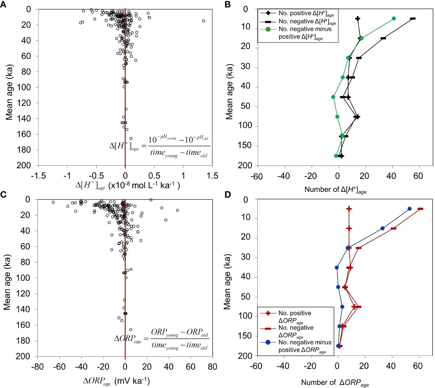
Figure 8 Sediment age distributions of the differences between two consecutive values down a core. Sediment age differences and distributions of positive and negative values in (A, B) Δ[H+]age and (C, D) ΔORPage (Supplementary Material Table S5). Positive (negative) Δ[H+]age and ΔORPage: increasing (decreasing) values with increasing sediment age. For Δ[H+]age and ΔORPage, there were 324 paired values from 93 cores, that is total of 121 cores with pH and ORP measurements, among which there were 93 core with at least 2 values for both pH and ORP measurements.
A relatively small fraction of the nSCS [H+]* profiles of were positive (17.5%, groups b and b’; Figure 6C), that is, [H+] along these cores was generally higher (and thus pH generally lower) than at the sediment subsurface. Two types of environmental factors could explain the occurrence of higher [H+] at depth than at subsurface, that is, characteristics of the ocean environment above the sediment, and chemical composition of the solid sediment.
Two characteristics of the first type were measured in this study, that is, water depth and bottom-water temperature. Contingency table analyses indicate that cores with positive [H+]* profiles were largely from shallower areas with higher bottom temperature (Supplementary Material Tables S6, S7). In the nSCS, subsurface-sediment pH is inversely related to water depth and directly related to bottom-water temperature (Shao et al., 2016), and consistently contingency table analysis showed correspondence of positive [H+]* profiles with higher subsurface-sediment pH (Supplementary Material Table S8).
Two characteristics of the second type were measured on some of our cores, that is, concentrations of OC and CaCO3. Contingency table analyses show correspondence of positive [H+]* cores with higher concentrations of sediment OC, and no relation with the concentrations of sediment CaCO3 (Supplementary Material Tables S9, S10). Hence, deep [H+]* higher than subsurface observed in 17.5% of the cores could reflect the in situ oxidation of higher concentrations of OC in the sediment of these generally shallower, higher bottom-water temperature areas.
Our findings on the vertical distributions of [H+] in the top ~10 m of nSCS sediment can be summarized as follows. The upper 2 m were the site of active geochemical processes that modified [H+] within 20-40 ka. These processes likely included redox reactions, ion diffusion, mineral dissolution, precipitation and authigenic processes (for example, carbonate dissolution/precipitation), and progressive consumption of OC by redox activity with increasing depth in the sediment. The [H+] characteristics of deeper, older sediment likely reflected continuous interactions between in situ geochemical diagenetic processes, which tended to create vertical variations, and vertical diffusion, which tended to even out vertical variability. In other words, deep sediment continued to experience in situ redox processes after the initial 20-40 ka, and the effects of redox processes were partly offset by vertical diffusion, that is, solid OC was progressively consumed as depth in the sediment increased, perhaps down to ~10 m (Figure 5H; Supplementary Material Table S9), and vertical diffusion partly evened out the resulting vertical variability in [H+] and thus pH.
In the literature, there is a report of vertical variations in nSCS sediment pH to much greater depths than this study’s ~10 m, that is, down to 795 m at ODP sites 1144 to 1148 (Figure 1), but the publication IODP-USIO (2020) does not provide explanations for these variations. Looking at the top ~10 m of the sediment in the present study provided a view of pH dynamics very different from that resulting from the usual focus on the top few centimeters. Our new understanding is also probably different from the view that will emerge from the more recent long cores obtained by ocean drilling. Our study identified a consistent [H+] difference between the upper 2 m of the sediment and underneath down to ~10 m that was previously unknown, and suggested that it could be explained by the combined actions of in situ geochemical diagenetic processes and vertical diffusion in the sediment.
We also observed large horizontal variations in the pH of subsurface and intermediate sediment (Figures 2A, B). Median pH values in the four regions generally increased eastwards in both subsurface and intermediate sediment, the highest values being in region K (Table 3).
Our results provide strong indications that pH values deep in the sediment were related to those at the sediment subsurface. First, there were corresponding areas of both low and high pH values in subsurface and deep sediments under the form of “chimneys” of vertically coherent pH from surface down (Figure 2D). Second, the differences between median intermediate and subsurface pH and [H+] were similar in core clusters 1 to 3 (Table 4), and thus independent of the absolute values of pH. Third, contingency table analysis showed an overall correspondence between the horizontal distribution of subsurface pH in the four regions (which were based on the horizontal distribution of subsurface pH) and the three core clusters (which were based on pH profiles), that is, the null hypothesis (H0: independence between regions and clusters) was rejected (p< 0.0001), cluster 1 being especially represented in region H, and cluster 3 in regions K and T (Supplementary Material Table S2; the correspondence between clusters and regions can be seen in Figure 4A). The process linking pH values deep in the sediment to those at the sediment subsurface was vertical diffusion, even if it did not dominate the vertical distribution of pH in most cores (Section 4.2). Hence, the characteristics of the overlying water column that affect the regional variability of surface-sediment pH identified by Shao et al. (2016) influenced the horizontal distribution of pH deep in the sediment.
In addition, higher pH was usually observed deep in the sediment than at subsurface in regions with higher concentrations of sediment OC (Supplementary Material Table S9). This suggests that the continuing remineralization of OC deposited from the overlying water onto the sediment in the past may influence the horizontal distribution of present deep sediment pH. Indeed, the analysis of the vertical variability of solid OC content in the sediment indicated that redox activity progressively consumed OC as depth in the sediment increased (Figure 5H).
In a previous paper (Shao et al., 2016), we had presented a conceptual model of the horizontal variations in subsurface-sediment pH in the nSCS. Here we propose a general conceptual model that combines the physical, chemical and biological factors that likely determined the distributions of pH with depth and sediment age in the upper ~10 m of the sediment (Figure 9). This model summarizes our previous and above findings concerning pH in subsurface and deeper sediment, respectively, in the nSCS during the last 200 ka.
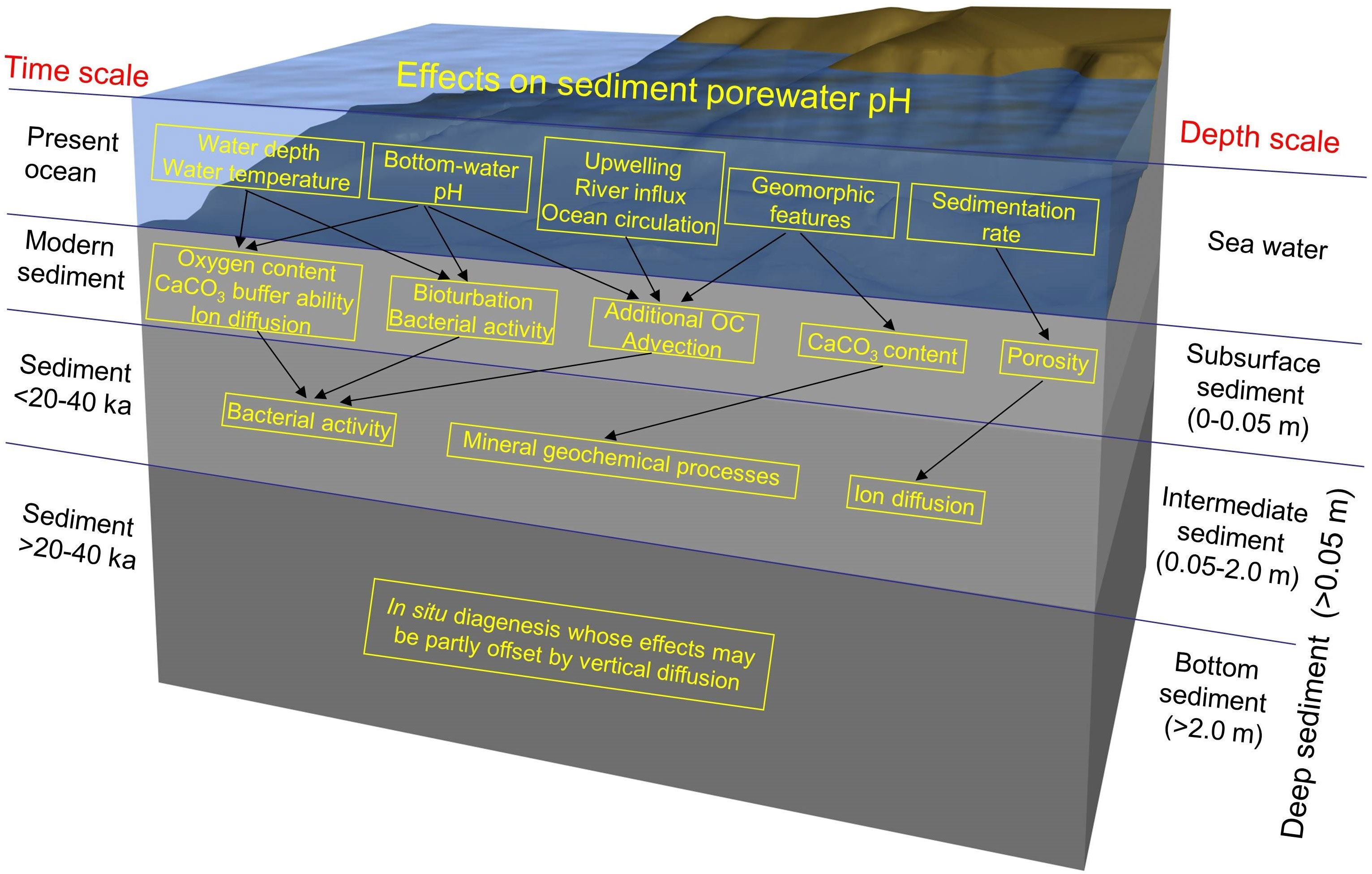
Figure 9 Conceptual model of the factors that likely determined the depth and sediment age distributions of pH in the nSCS during the last 200 ka. Details are provided in the text.
First in modern sediment (top centimeters), the most important sources of porewater H+ are organic carbon (OC) redox processes (Hales and Emerson, 1996; Reimers et al., 1996; Jourabchi et al., 2005). Most of the OC is oxidized in the upper few centimeters of the sediment, primarily utilizing dissolved O2 (Emerson and Bender, 1981; Reimers et al., 1996), and the environment beneath the oxygen-containing layer is anoxic. In the anoxic sediment layer, the evolution of pH depends on such diagenetic processes as diffusion, sulfate reduction, denitrification, manganese reduction, iron reduction, and AOM (Soetaert et al., 2007; Turchyn and DePaolo, 2011). Hydrostatic pressure (water depth) as well as bottom-water temperature and pH affect subsurface-sediment pH through mechanisms that include redox processes (oxygen content) (Jourabchi et al., 2005), the dissolution constants and buffering capacity of CaCO3 (Culberson and Pytkowicz, 1968; Gieskes, 1969), ion diffusion (Li and Gregory, 1974), bioturbation (Trevors, 1985; Arnosti et al., 1998; Atkinson et al., 2007; Widdicombe et al., 2009), and bacterial activity (Cragg et al., 1999; Jourabchi et al., 2005; Zhu et al., 2006). Recent-sediment pH also reflects differences in geomorphic features (Shao et al., 2016), sedimentation rates (Jourabchi et al., 2005) and water-column circulation characteristics, which include upwelling, river influx and ocean currents (Shao et al., 2016). These factors influence subsurface-sediment pH through OC supply for redox activity, advection, and the CaCO3 content and porosity of the sediment.
Second in sediment<20-40 ka (upper 2 m below the sediment subsurface), pH is affected by geochemical reactions that occur in situ over time, and the downward transfer of dissolved chemical species by both diffusion and porewater advection (Li and Gregory, 1974; Boudreau, 1997; Cai et al., 2000; Jourabchi et al., 2005; Stahl et al., 2006). The intermediate-sediment pH is also influenced by bacterial redox activity (Ben-Yaakov, 1973; Nealson, 1997; Jourabchi et al., 2005), and mineralogical reactions (Berner, 1980).
Third in older sediment (>20-40 ka, between 2 and about 10 m), the geochemical characteristics are generally more stable down to 200 ka but generally not uniform with depth, due to in situ diagenesis whose effects are partly offset by vertical diffusion (Berner, 1980; Parkes et al., 1990; Turchyn and DePaolo, 2011).
This conceptual model provides a framework for further studies of sediment pH in the top multi-meter layer of sediments in the World Ocean.
We analyzed the spatial and geological time-scale variability of sediment pH in the top ~10 m of the sediment (down to 11.9 m) in the deep-sea environment of the northern South China Sea. Our results showed a marked downward increase in pH in the upper 2 m of the sediment (first 20-40 ka). In older (>20-40 ka), bottom (>2 m) sediment, the geochemical characteristics were more stable. The first 20-40 ka, upper 2-m layer of the sediment was thus the geochemically active period and layer. The significant decrease of sediment pH in this layer indicated that the hydrogen ion producing reactions were increasingly replaced by hydrogen ion consuming reactions. Below this layer, the weaker redox activity corresponded to the decreased content in OC, which was progressively consumed with increasing depth and time.
The observed strong increase in pH with depth in the top 10 m of the sediment is not consistent the hypothesis found in the literature that diffusion controls, and thus uniforms, the depth distribution of pH below the top few centimeters (i.e. oxic zone) of the sediment.
The original contributions presented in the study are included in the article/Supplementary Material. Further inquiries can be directed to the corresponding author.
CS, DT, and LL designed and performed the research, and analyzed the data. CS, DT, LL, YS and HW wrote the paper. All authors contributed to the article and approved the submitted version.
The present work received funding from: Guangdong Special Support Program (2019BT02H594), Key Special Project of Southern Marine Science and Engineering Guangdong Laboratory (Guangzhou) for Introduced Talents Team, (GML2021GD0810), the National Natural Science Foundation of China (Project 41876136, Key Project 41430968); the Cooperation Project (DD20191037, 2022R-SYS25-03), the 2022 Research Program of Sanya Yazhou Bay Science and Technology City (SKJC-2022-01-001); and the National key R&D program of China (2018YFC0310000) awarded to HW; and the cooperation agreement between the Chinese Academy of Sciences and the French Centre National de la Recherche Scientifique (DT and LL).
We thank Profs. Bernard Boudreau, Dalhousie University, Canada, and Jean-Pierre Gattuso and Nathalie Vigier, Villefranche Oceanography Laboratory, France, for useful suggestions at early writing stages of this work. We also thank the two Frontiers in Marine Science reviewers for their very useful comments and suggestions.
The authors declare that the research was conducted in the absence of any commercial or financial relationships that could be construed as a potential conflict of interest.
All claims expressed in this article are solely those of the authors and do not necessarily represent those of their affiliated organizations, or those of the publisher, the editors and the reviewers. Any product that may be evaluated in this article, or claim that may be made by its manufacturer, is not guaranteed or endorsed by the publisher.
The Supplementary Material for this article can be found online at: https://www.frontiersin.org/articles/10.3389/fmars.2023.1126704/full#supplementary-material
Adkins J. F., McIntyre K., Schrag D. P. (2002). The salinity, temperature, and δ18O of the glacial deep ocean. Science. 298, 1769–1773. doi: 10.1126/science.1076252
Archer D., Emerson S., Reimers C. (1989). Dissolution of calcite in deep-sea sediments: pH and O2 microelectrode results. Geochim. Cosmochim. Acta 53, 2831–2845. doi: 10.1016/0016-7037(89)90161-0
Arnosti C., Jørgensen B., Sagemann J., Thamdrup B. (1998). Temperature dependence of microbial degradation of organic matter in marine sediments: Polysaccharide hydrolysis, oxygen consumption, and sulfate reduction. Mar. Ecol. Prog. Ser. 165, 59–70. doi: 10.3354/meps165059
Atkinson C. A., Jolley D. F., Simpson S. L. (2007). Effect of overlying water pH, dissolved oxygen, salinity and sediment disturbances on metal release and sequestration from metal contaminated marine sediments. Chemosphere. 69, 1428–1437. doi: 10.1016/j.chemosphere.2007.04.068
Ben-Yaakov S. (1973). pH buffering of pore water of recent anoxic marine sediments. Limnol. Oceanogr. 18, 86–94. doi: 10.4319/lo.1973.18.1.0086
Berner R. A. (1980). Early diagenesis: A theoretical approach (Princeton: Princeton University Press).
Blake R. C., Shute E. A., Greenwood M. M., Spencer G. H., Ingledew W. J. (1993). Enzymes of aerobic respiration on iron. FEMS Microbiol. Rev. 11, 9–18. doi: 10.1111/j.1574-6976.1993.tb00261.x
Blouet J.-P., Arndt S., Imbert P., Regnier P. (2021). Are seep carbonates quantitative proxies of CH4 leakage? Modeling the influence of sulfate reduction and anaerobic oxidation of methane on pH and carbonate precipitation. Chem. Geology. 577, 120254. doi: 10.1016/j.chemgeo.2021.120254
Burdige D. J., Zimmerman R. C., Hu X. (2008). Rates of carbonate dissolution in permeable sediments estimated from pore-water profiles: The role of sea grasses. Limnol. Oceanogr. 53, 549–565. doi: 10.4319/lo.2008.53.2.0549
Cai W.-J. (1992). In situ microelectrode studies of the hemipelagic sediments of the northeast pacific ocean (San Diego: Univ. California).
Cai W.-J., Chen F., Powell E. N., Walker S. E., Parsons-Hubbard K. M., Staff G. M., et al. (2006). Preferential dissolution of carbonate shells driven by petroleum seep activity in the gulf of Mexico. Earth Planet Sci. Lett. 248, 227–243. doi: 10.1016/j.epsl.2006.05.020
Cai W.-J., Reimers C. E. (1993). The development of pH and pCO2 microelectrodes for studying the carbonate chemistry of pore waters near the sediment-water interface. Limnol. Oceanogr. 38, 1762–1773. doi: 10.4319/lo.1993.38.8.1762
Cai W.-J., Reimers C. E., Shaw T. (1995). Microelectrode studies of organic carbon degradation and calcite dissolution at a California continental rise site. Geochim. Cosmochim. Acta 59, 497–511. doi: 10.1016/0016-7037(95)00316-R
Cai W.-J., Zhao P., Wang Y. (2000). pH and pCO2 microelectrode measurements and the diffusive behavior of carbon dioxide species in coastal marine sediments. Mar. Chem. 70, 133–148. doi: 10.1016/S0304-4203(00)00017-7
Cragg B., Law K., O’Sullivan G., Parkes R. (1999). “34.Bacterial profiles in deep sediments of the alboran Sea, western Mediterranean, sites 976-978,” in Proceedings of the ocean drilling program: Scientific results. ocean drilling program. Eds. Zahn R., Comas M., Klaus A. (Ocean Drilling Program), 433–438. doi: 10.2973/odp.proc.sr.161.267.1999
Culberson C., Pytkowicz R. M. (1968). Effect of pressure on carbonic acid, boric acid, and the pH in seawater. Limnol. Oceanogr. 13, 403–417. doi: 10.4319/lo.1968.13.3.0403
Drupp P. S., De Carlo E. H., Mackenzie F. T. (2016). Porewater CO2–carbonic acid system chemistry in permeable carbonate reef sands. Mar. Chem. 185, 48–64. doi: 10.1016/j.marchem.2016.04.004
Emerson S. R., Bender M. (1981). Carbon fluxes at the sediment-water interface of the deep-sea: Calcium carbonate preservation. J. Mar. Res. 39, 139–162.
Emerson S., Grundmanis V., Graham D. (1982). Carbonate chemistry in marine pore waters: MANOP sites c and s. Earth Planet Sci. Lett. 61, 220–232. doi: 10.1016/0012-821X(82)90055-3
Emerson S., Jahnke R., Bender M., Froelich P., Klinkhammer G., Bowser C., et al. (1980). Early diagenesis in sediments from the eastern equatorial pacific, i. pore water nutrient and carbonate results. Earth Planet Sci. Lett. 49, 57–80. doi: 10.1016/0012-821X(80)90150-8
Expedition 302 Scientists (2006). “Methods,” in Proceedings of the integrated ocean drilling program. Eds. Backman J., Moran K., McInroy D. B., Mayer L. A. (Tokyo: Integrated Ocean Drilling Program Management International, Inc).
Expedition 329 Scientists (2011). “Methods,” in Proceedings of the integrated ocean drilling program. Eds. Hondt S.D’, Inagaki F., Alvarez Zarikian C. A. (Tokyo: Integrated Ocean Drilling Program Management International, Inc).
Fassbender A. J., Orr J. C., Dickson A. G. (2021). Technical note: Interpreting pH changes. Biogeosciences. 18, 1407–1415. doi: 10.5194/bg-18-1407-2021
Fisher J. B., Matisoff G. (1981). High resolution vertical profiles of pH in recent sediments. Hydrobiologia. 79, 277–284. doi: 10.1007/BF00006325
Gieskes J. M. (1969). Effect of temperature on the pH of seawater. Limnol. Oceanogr. 14, 679–685. doi: 10.4319/lo.1969.14.5.0679
Hales B., Emerson S. (1996). Calcite dissolution in sediments of the ontong-Java plateau: In situ measurements of pore water O2 and pH. Global Biogeochemical Cycles. 10, 527–541. doi: 10.1029/96GB01522
Hales B., Emerson S. (1997). Calcite dissolution in sediments of the ceara rise: In situ measurements of porewater O2, pH, and CO2(aq). Geochim. Cosmochim. Acta 61, 501–514. doi: 10.1016/S0016-7037(96)00366-3
Hales B., Emerson S., Archer D. (1994). Respiration and dissolution in the sediments of the western north Atlantic: Estimates from models of in situ microelectrode measurements of porewater oxygen and pH. Deep Sea Res. Part I: Oceanographic Res. Papers. 41, 695–719. doi: 10.1016/0967-0637(94)90050-7
Hansson I. (1973). A new set of pH-scales and standard buffers for sea water. Deep Sea Res. Oceanographic Abstracts. 20, 479–491. doi: 10.1016/0011-7471(73)90101-0
Herlihy A. T., Mills A. L. (1986). The pH regime of sediments underlying acidified waters. Biogeochemistry. 2, 95–99. doi: 10.1007/BF02186967
Hunting E. R., Kampfraath A. A. (2013). Contribution of bacteria to redox potential (Eh) measurements in sediments. Int. J. Environ. Sci. Technology. 10, 55–62. doi: 10.1007/s13762-012-0080-4
IODP-USIO (2020). Core database. U.S. implementing organization (IODP-USIO). Available at: http://iodp.tamu.edu/janusweb/chemistry/chemiw.cgi.
Jahnke R., Heggie D., Emerson S., Grundmanis V. (1982). Pore waters of the central pacific ocean: Nutrient results. Earth Planet Sci. Lett. 61, 233–256. doi: 10.1016/0012-821X(82)90056-5
Jourabchi P., Van Cappellen P., Regnier P. (2005). Quantitative interpretation of pH distributions in aquatic sediments: A reaction-transport modeling approach. Am. J. Sci. 305, 919–956. doi: 10.2475/ajs.305.9.919
Li Y.-H., Gregory S. (1974). Diffusion of ions in sea water and in deep-sea sediments. Geochim. Cosmochim. Acta 38, 703–714. doi: 10.1016/0016-7037(74)90145-8
Lisiecki L., Raymo M. (2005). A Pliocene-Pleistocene stack of 57 globally distributed benthic 18O records. Paleoceanography 20: PA. 1003, 1–17. doi: 10.1594/PANGAEA.704257
Luo X., Xu X., Zhang Z., Chen Z. (2007). Development and technical character of XXG-T marine geothermal gradient measurement system. Geological Res. South China Sea. 00, 102–110.
Ma Y. A., Xu H. Z., Yu T., He G. K., Zhao Y. Y., Fu Y. Z. (2008). The specification for marine monitoring-part 5: Sediment analysis (Beijing: China Standardization Press).
Martin K. M., Wood W. T., Becker J. J. (2015). A global prediction of seafloor sediment porosity using machine learning. Geophysical Res. Letters. 42, 10,640–610,646. doi: 10.1002/2015GL065279
Miao X., Feng X., Liu X., Li J., Wei J. (2021). Effects of methane seepage activity on the morphology and geochemistry of authigenic pyrite. Mar. Pet. Geol. 133, 105231. doi: 10.1016/j.marpetgeo.2021.105231
Miao X., Liu X., Li Q., Li A., Cai F., Kong F., et al. (2022). Porewater geochemistry indicates methane seepage in the Okinawa trough and its implications for the carbon cycle of the subtropical West pacific. Palaeogeography Palaeoclimatology Palaeoecology. 607, 111266. doi: 10.1016/j.palaeo.2022.111266
Murray J. W., Emerson S., Jahnke R. (1980). Carbonate saturation and the effect of pressure on the alkalinity of interstitial waters from the Guatemala basin. Geochim. Cosmochim. Acta 44, 963–972. doi: 10.1016/0016-7037(80)90285-9
Nealson K. H. (1997). Sediment bacteria: Who’s there, what are they doing, and what’s new? Annu. Rev. Earth Planet Sci. 25, 403–434. doi: 10.1146/annurev.earth.25.1.403
Parkes R. J., Cragg B. A., Fry J. C., Herbert R. A., Wimpenny J. W. T., Allen J. A., et al. (1990). Bacterial biomass and activity in deep sediment layers from the Peru margin [and discussion]. Philos. Trans. R. Soc. London Ser. A. 331, 139–153. doi: 10.1098/rsta.1990.0061
Reimers C. E., Ruttenberg K. C., Canfield D. E., Christiansen M. B., Martin J. B. (1996). Porewater pH and authigenic phases formed in the uppermost sediments of the Santa Barbara basin. Geochim. Cosmochim. Acta 60, 4037–4057. doi: 10.1016/S0016-7037(96)00231-1
Schulz H. D., Dahmke A., Schinzel U., Wallmann K., Zabel M. (1994). Early diagenetic processes, fluxes, and reaction rates in sediments of the south Atlantic. Geochim. Cosmochim. Acta 58, 2041–2060. doi: 10.1016/0016-7037(94)90284-4
Shao C., Sui Y., Tang D., Legendre L. (2016). Spatial variability of surface-sediment porewater pH and related water-column characteristics in deep waters of the northern south China Sea. Prog. Oceanogr. 149, 134–144. doi: 10.1016/j.pocean.2016.10.006
Soetaert K., Hofmann A. F., Middelburg J. J., Meysman F. J. R., Greenwood J. (2007). The effect of biogeochemical processes on pH. Mar. Chem. 105, 30–51. doi: 10.1016/j.marchem.2006.12.012
Stahl H., Glud A., Schröder C. R., Klimant I., Tengberg A., Glud R. N. (2006). Time-resolved pH imaging in marine sediments with a luminescent planar optode. Limnology Oceanography: Methods 4, 336–345. doi: 10.4319/lom.2006.4.336
Trevors J. T. (1985). Effect of temperature on selected microbial activities in aerobic and anaerobically incubated sediment. Hydrobiologia. 126, 189–192. doi: 10.1007/BF00008686
Turchyn A. V., DePaolo D. J. (2011). Calcium isotope evidence for suppression of carbonate dissolution in carbonate-bearing organic-rich sediments. Geochim. Cosmochim. Acta 75, 7081–7098. doi: 10.1016/j.gca.2011.09.014
Ullman W. J., Aller R. C. (1982). Diffusion coefficients in nearshore marine sediments. Limnol. Oceanogr. 27, 552–556. doi: 10.4319/lo.1982.27.3.0552
Wang S. M., Yan W. H., Zheng C. J., Dong G. X. (2010). Method for chemical analysis of rocks and ores-general rulers and regulatons (Beijing: China Standardization Press).
Wenzhöfer F., Adler M., Kohls O., Hensen C., Strotmann B., Boehme S., et al. (2001). Calcite dissolution driven by benthic mineralization in the deep-sea: in situ measurements of Ca2+, pH, pCO2 and O2. Geochim. Cosmochim. Acta 65, 2677–2690. doi: 10.1016/S0016-7037(01)00620-2
Widdicombe S., Dashfield S. L., McNeill C. L., Needham H. R., Beesley A., McEvoy A., et al. (2009). Effects of CO2 induced seawater acidification on infaunal diversity and sediment nutrient fluxes. Mar. Ecol. Prog. Ser. 379, 59–75. doi: 10.3354/meps07894
Widdicombe S., Spicer J. (2011). “Effects of ocean acidification on sediment fauna,” in Ocean acidification (Oxford: Oxford Scholarship Online), 176–191.
Yan M. H., Huang H. P. (1993). Method for chemical analysis of rocks and ores-general rules and regulations (Beijing: China Standardization Press).
Yanagawa K., Morono Y., de Beer D., Haeckel M., Sunamura M., Futagami T., et al. (2013). Metabolically active microbial communities in marine sediment under high-CO2 and low-pH extremes. ISME J. 7, 555–567.
Zhang W. Y., Zhang C. M., Xu K. C., Wang H. C., Chen B. L., Gu G. L. (1998). The specification for marine monitoring-part 5: Sediment analysis (Beijing: China Standardization Press).
Zhu Q., Aller R. C., Fan Y. (2006). Two-dimensional pH distributions and dynamics in bioturbated marine sediments. Geochim. Cosmochim. Acta 70, 4933–4949. doi: 10.1016/j.gca.2006.07.033
Keywords: sediment pH, Northern South China Sea, ~10 m sediment cores, ancient ocean, diagenetic processes
Citation: Shao C, Tang D, Legendre L, Sui Y and Wang H (2023) Vertical distribution of pH in the top ~10 m of deep-ocean sediments: Analysis of a unique dataset. Front. Mar. Sci. 10:1126704. doi: 10.3389/fmars.2023.1126704
Received: 18 December 2022; Accepted: 21 February 2023;
Published: 27 March 2023.
Edited by:
Elva G. Escobar-Briones, National Autonomous University of Mexico, MexicoReviewed by:
Ligia Perez-Cruz, National Autonomous University of Mexico, MexicoCopyright © 2023 Shao, Tang, Legendre, Sui and Wang. This is an open-access article distributed under the terms of the Creative Commons Attribution License (CC BY). The use, distribution or reproduction in other forums is permitted, provided the original author(s) and the copyright owner(s) are credited and that the original publication in this journal is cited, in accordance with accepted academic practice. No use, distribution or reproduction is permitted which does not comply with these terms.
*Correspondence: DanLing Tang, bGluZ3ppc3RkbEAxMjYuY29t
Disclaimer: All claims expressed in this article are solely those of the authors and do not necessarily represent those of their affiliated organizations, or those of the publisher, the editors and the reviewers. Any product that may be evaluated in this article or claim that may be made by its manufacturer is not guaranteed or endorsed by the publisher.
Research integrity at Frontiers
Learn more about the work of our research integrity team to safeguard the quality of each article we publish.