 Huanhai Yang
 Mingyu Sun2
- 1School of Computer Science and Technology, Shandong Technology and Business University, Yantai, Shandong, China
- 2College of Foreign Studies, Shandong Technology and Business University, Yantai, Shandong, China
- 3The Second Medical College, Binzhou Medical University, Yantai, Shandong, China
Dissolved oxygen is an important water quality indicator that affects the health of aquatic products in aquaculture, and its monitoring and prediction are of great significance. To improve the prediction accuracy of dissolved oxygen water quality series, a hybrid prediction model based on variational mode decomposition (VMD) and a deep belief network (DBN) optimized by an improved slime mould algorithm (SMA) is proposed in this paper. First, VMD is used to decompose the nonlinear dissolved oxygen time series into several relatively stable intrinsic mode function (IMF) subsequences with different frequency scales. Then, the SMA is improved by applying elite opposition-based learning and nonlinear convergence factors to increase its population diversity and enhance its local search and global convergence capabilities. Finally, the improved SMA is used to optimize the hyperparameters of the DBN, and the aquaculture water quality prediction VMD-ISMA-DBN model is constructed. The model is used to predict each IMF subsequence, and the ISMA optimization algorithm is used to adaptively select the optimal hyperparameters of the DBN model, and the prediction results of each IMF are accumulated to obtain the final prediction result of the dissolved oxygen time series. The dissolved oxygen data of aquaculture water from 8 marine ranches in Shandong Province, China were used to verify the prediction performance of the model. Compared with the stand-alone DBN model, the prediction performance of the model has been significantly improved, MAE and MSE have been reduced by 43.28% and 40.43% respectively, and (R2) has been increased by 8.37%. The results show that the model has higher prediction accuracy than other commonly used intelligent models (ARIMA, RF, TCN, ELM, GRU and LSTM); hence, it can provide a reference for the accurate prediction and intelligent regulation of aquaculture water quality.
1 Introduction
In the field of aquaculture, the quality of water is an important factor affecting the growth, development and reproduction of aquatic organisms. Water quality is unstable and constantly changing due to factors such as weather, breeding density, fish activity and fishermen intervention. In aquaculture, it is necessary to ensure that the dissolved oxygen content, pH value, water temperature, salinity and other water quality indicators are within the normal ranges. Taking the dissolved oxygen content as an example, the suitable dissolved oxygen content for fish is above 3 mg/L. When the dissolved oxygen content is less than 3 mg/L, the fish will stop eating, and if the dissolved oxygen content is too high, the fish may suffer from bubble disease. Therefore, accurate prediction and timely intervention of water quality indicators to control the aquaculture water environment within an appropriate range are of great significance to ensure the healthy growth of fish.
In recent years, many scholars have done a lot of research on water quality prediction, and applied various models to improve prediction accuracy. Existing water quality prediction models mainly include regression analysis based on mathematical statistics (Areerachakul et al. (2013); Brooks et al. (2016)) and methods based on computational intelligence (Rajaee et al. (2020)). Traditional prediction methods based on regression analysis have high requirements on the distribution of data samples, and a large amount of data is required for training during modeling, which affects the efficiency and accuracy of prediction. Prediction methods based on computational intelligence (machine learning and deep learning) have the characteristics of autonomous learning, optimal calculation, and strong nonlinear fitting capabilities, and are more suitable for predictive modeling of nonlinear aquaculture water quality data. Many scholars have carried out much research on the application of intelligent algorithms to solve the problem of aquaculture water quality prediction and have built a variety of intelligent prediction models based on machine learning algorithms. Examples include genetic programming (Jafari et al. (2020)), general regression neural network (GRNN) (Antanasijević et al. (2014)), autoregressive integrated moving average model (ARIMA) (Xuan et al. (2021)), tree-based artificial intelligence models (Tiyasha et al. (2021)), radial basis function neural networks (Rozario and Devarajan (2021)), fuzzy neural network (Ren et al. (2018)) and Bayesian model averaging (Kisi et al. (2020)). Due to the excellent performance of the deep learning framework in time series forecasting, especially in long-term forecasting, most scholars have studied the application of deep learning methods in water quality forecasting. Examples include convolutional neural network (Ta and Wei (2018)), long short-term memory (Barzegar et al. (2020)), gated recurrent unit neural network (Cao et al. (2020)), bidirectional simple recurrent units (Chen et al. (2022)) and temporal convolutional network (Li et al. (2022b)).
The above intelligent prediction models, combined with the advantages of strong self-adaptation and the generalization ability of machine learning, have achieved good results in the prediction of nonlinear water quality data. Deep belief network (DBN) has the advantages of requiring less training time, effectively extracting data features, reducing the feature dimension and does not easily fall into local optima. DBN have been widely used in emotion recognition (Hassan et al., 2019), time series prediction (Kuremoto et al., 2014), text classification (Jiang et al., 2018) medical diagnosis (Khatami et al., 2017), etc. This paper studies the application of a DBN to accurately predict the development trend of aquaculture water quality.
Dissolved oxygen and other water quality data in aquaculture are affected by many factors, such as chemical reactions, biological activities, meteorological changes, and fishermen intervention, and have the characteristics of nonlinearity, easily changing, and noise. To improve the accuracy and stability of prediction results, most scholars use the method of data decomposition to process a water quality time series as the input sample of a prediction model. The time series decomposition algorithms include empirical mode decomposition (EMD), ensemble empirical mode decomposition (EEMD), complete EEMD with adaptive noise (CEEMDAN), variational mode decomposition (VMD) and others. (Zhang et al., 2021; Zhang et al., 2022) constructed decomposition-ensemble frameworks based on EMD to predict water quality (suspended sediment concentration, SSC) time series, and achieved high prediction accuracy. Liu et al. (2016) applied EMD and a back-propagation neural network (BPNN) to predict water temperature in aquaculture. Huan et al. (2018) and Li et al. (2018) applied EEMD to extract multiscale features from water quality data before making predictions. Lu and Ma (2020) proposed two hybrid short-term dissolved oxygen water quality prediction models, CEEMDAN-XGBoost and CEEMMDAN-RF. Huang et al. (2021) proposed an interval dissolved oxygen water quality prediction method based on VMD and a deep autoregressive recurrent neural network (DeepAR). Ren et al. (2020) applied VMD to decompose dissolved oxygen time series as input samples for the DBN prediction model. Pipelzadeh and Mastouri (2021) implemented a water quality prediction model based on VMD and model tree (MT) to predict total dissolved solids (TDS) and electrical conductivity (EC) water quality parameters. Bi et al. (2023) used VMD to process non-stationary water quality time series to improve prediction accuracy. VMD determines the frequency center and bandwidth of each component by iteratively searching for the optimal solution of the variational mode, prevents mode aliasing by controlling the bandwidth and has strong robustness to sampling and denoising. This paper studies the application of VMD to decompose aquaculture water quality signals to reduce the influence of nonlinear and nonstationary characteristics of the data on the performance of the prediction model and to improve the prediction accuracy.
Most of the intelligent models based on neural networks have shortcomings, such as difficulty in determining hidden neurons, overlearning or under learning, and easily falling into local optima. Moreover, the improper selection of hyperparameters of intelligent models also reduces the prediction accuracy of the model. Therefore, many scholars have studied and applied meta-heuristics algorithm to optimize the hyperparameters of neural network prediction models. Meta-heuristics algorithms mainly include evolutionary algorithms, swarm intelligence algorithms that simulate biological survival, and algorithms that simulate physical phenomena. Evolutionary algorithms draw on the evolutionary process of organisms in nature, including basic operations such as genetic encoding, population initialization and crossover mutation operator. Genetic algorithm (GA) and differential evolution algorithm (DE) are two commonly used evolutionary algorithms (Hu et al., 2022). The optimization algorithms inspired by physical phenomena and designed according to the laws of physics include gravitational search algorithm m (GSA) (Rashedi et al., 2009), gradient-based optimizer (GBO) (Ahmadianfar et al., 2020) and atom search optimization (ASO) (Zhao et al., 2019), etc (Emam et al., 2023). The swarm intelligence optimization algorithm is an intelligent algorithm that simulates the behavior of groups of fish, birds, wolves of bacteria in nature and uses information exchange and cooperation between groups to achieve optimization purposes (Wang et al., 2022). Swarm intelligence algorithms that have been widely used in recent years include monarch butterfly optimization (MBO)(Wang et al., 2019), hunger games search (HGS) (Yang et al., 2021), sparrow search algorithm (SSA) (Xue and Shen, 2020), dingoes hunting strategy (DHS) (Peraza-Vázquez et al., 2021), bald eagle search (BES) (Alsattar et al., 2020), Wild horse optimizer (WHO) (Naruei and Keynia, 2021), whale optimization algorithm (WOA) (Mirjalili and Lewis, 2016), colony predation algorithm (CPA)(Yang et al., 2021), weighted mean of vectors (INFO) (Ahmadianfar et al., 2022), harris hawks optimization (HHO) 109 (Heidari et al., 2019) and slime mould algorithm (SMA) (Li et al., 2020). The slime mould optimization algorithm is an optimization algorithm proposed according to the vegetative growth process of a slime mould. The algorithm has the advantages of a simple structure, fast convergence speed, strong local search ability and relatively stable effect. In this paper, the optimization performance of the SMA is further improved, the improved SMA (ISMA) is used to optimize the hyperparameters of the DBN prediction model, and the optimal hyperparameter combination is used to construct the aquaculture water quality prediction model to achieve accurate prediction of water quality time series.
The main contributions of this paper include the following four points:
(1) In this paper, the multiscale decomposition of the water quality signal is carried out by VMD to reduce the complexity of the nonlinear dissolved oxygen time series, and the relatively stable subsequence is used to train the prediction model to improve the prediction accuracy.
(2) To set the number of VMD modes more reasonably, this paper calculates the mean absolute error (MAE) between the original signal and the decomposed mode reconstruction sequence and determines the mode decomposition number according to the change trend of the MAE value to prevent information loss and mode aliasing.
(3) In this paper, elite opposition-based learning and improved nonlinear convergence factors are used to improve the SMA with multiple strategies, which improves the diversity of the initial population of the algorithm, balances the global search ability and local search ability of the algorithm, and makes it have better convergence accuracy and stability.
(4) Through the ISMA, the training process of the DBN neural network is optimized to obtain the best parameter combination, which makes the model structure more reasonable and greatly improves the prediction accuracy of the time series.
2 Material and methods
2.1 Study area and data source
In this paper, the time series of dissolved oxygen in aquaculture water of marine ranches in Shandong Province, China, was used as a data sample to construct an accurate water quality prediction model. In recent years, Shandong Province has vigorously developed the construction of marine ranching, and more than 150 high-quality marine ranching projects have been built thus far. The authors of this paper deployed water quality sensors in 8 marine ranches on the Shandong Peninsula and established multiple aquaculture water quality data collection networks. Starting from June 2020, time series data, such as dissolved oxygen, pH, salinity, and water temperature, for aquaculture water quality indicators were collected year round, and the data were collected every ten minutes. Figure 1 shows the approximate locations of the marine ranches where water quality data were collected. Table 1 shows the descriptive statistics of the dissolved oxygen time series collected from 8 marine ranches from June 1, 2021 to July 1, 2022.
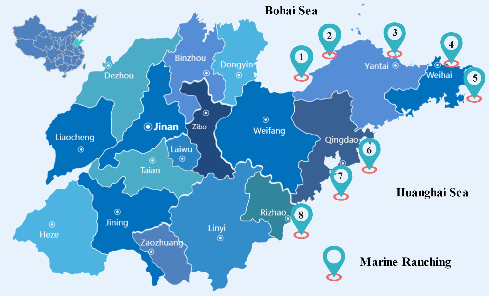
Figure 1 Approximate location of marine ranches where water quality data was collected.
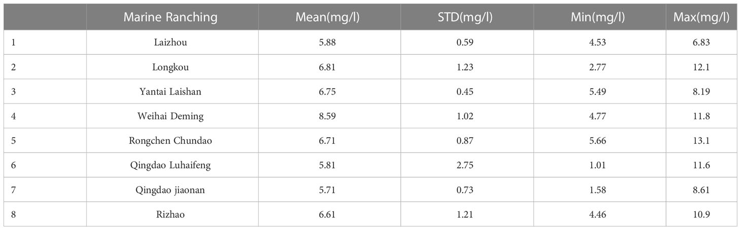
Table 1 Descriptive statistics of dissolved oxygen time series collected from 8 marine ranches.
2.2 Variational mode decomposition
VMD is an adaptive, completely non recursive variational mode signal decomposition method that determines the frequency center and bandwidth of each component by iteratively searching for the optimal solution of the variational model. The nonstationary time series is decomposed into relatively stationary intrinsic mode function (IMF) subsequences with different frequency scales. The center frequency of
each subsequence is . The constraint condition is that the sum of the IMF components is equal to the original signal. The specific construction steps are as follows:
(1) Obtain the signal of each IMF component through the Hilbert transform, calculate its unilateral spectrum, and use exponential correction to modulate the spectrum of each mode function to the corresponding baseband [13], as shown in the following equation (1).
In the above formula, represents the k IMF components obtained by the decomposition process, and represents the center frequency of each component, is a generalized function, that is, the Dirac delta function, is the imaginary unit, and exponential correction is used to modulate the spectrum of each mode function to the corresponding fundamental frequency band (Niu et al., 2020).
(2) Calculate the square of the norm of the gradient of the demodulated signal and perform Gaussian smoothing to obtain the bandwidth of each mode signal, as shown in the following equation (2)
In the above formula, indicates 2-norm processing and is the convolution operation.
(3) When construct a variational problem, the sum of the estimated bandwidths of each mode is the smallest, the constraint condition is that the sum of all modes is equal to the original signal , and the corresponding constraint variational expression is shown in equation (3).
(4) To find the optimal solution of the constrained variational problem, the augmented Lagrangian function is introduced by taking advantage of the quadratic penalty term and the Lagrangian multiplier to transform the constrained variational problem into an unconstrained variational problem, as shown in Equation (4).
In the above formula, is the quadratic penalty term, which can ensure the accuracy of signal reconstruction in a Gaussian noise environment. is the Lagrangian multiplication operator, which can maintain the strictness of the constraints (Dragomiretskiy and Zosso, 2014; Yang and Liu, 2022).
(5) Use the alternating direction method of multipliers (ADMM) to iteratively solve each IMF component and its corresponding center frequency . The formulas are (5) and (6), respectively.
where w is the frequency, is the Fourier transform of the original signal f(t), and and are the Fourier transforms of and , respectively.
2.3 Slime mould algorithm
The SMA was proposed by Li et al. in 2020. The algorithm mainly simulates the behavior and morphological changes in slime moulds during foraging foraging (Li et al., 2020). The slime mould judges the location of the food according to the concentration of the food. The higher the concentration of food is, the stronger the propagating waves generated by the biological oscillator in the body. This causes an increase in the width of the veins, forming a network of veins with different thicknesses between multiple food sources and establishing the best path for finding food. In addition, after the slime mould obtains food, there is still a certain probability of searching the unknown area (Zubaidi et al., 2020). The position update formula of a slime mould individual is shown in (7).
Among them, and represent the upper and lower boundaries of the search range, is a random oscillation ranging from -a to a and gradually approaches 0 as the number of iterations increases, oscillates from -1to 1 and finally tends to 0. Moreover, represents a random value in the [0,1] interval, z is a custom parameter that represents the proportion of randomly distributed slime mould individuals to the population and is generally 0.03, t is the current iteration number, and represents the slime mould individual with the best fitness. represents the position of the current iteration of the slime mould individual, and and are the positions of two random individuals. represents the weight coefficient.
The update formulas of the control parameter , parameter and parameter in formula (7) are formulas (8), (9) and (10), respectively.
In the above formula, is the number of slime mould populations, and represents the fitness value of the i-th slime mould individual. is the current optimal fitness value. The function is a nonlinear activation function whose output value is in the interval [-1,1].
In the above formula, is the current number of iterations, and is the maximum number of iterations. The function is the reverse hyperbolic tangent function.
The value of oscillates in the interval , and the synergy between and simulates the selection behavior of slime moulds. The weight coefficient of slime mould individuals is related to their fitness value. The weight formula of individuals whose fitness value sequence is in the top 50% in the slime mould population is provided in (11).
The weight coefficient formula of other slime mould individuals is provided in (12).
In Equations (11) and (12), represents a random number ranging from 0 to 1, and and represent the best and worst fitness values for the current iteration, respectively.
2.4 Deep belief network
A DBN is a deep neural network composed of multiple layers of restricted Boltzmann machines (RBMs) and one layer of a back propagation (BP) neural network (Hinton and Salakhutdinov, 2006; Hinton et al., 2006). The RBM consists of a visible layer and a hidden layer. In the DBN structure, the hidden layer of the bottom RBM is the visible layer of the next RBM, and the output of the last RBM is used as the input of the BP neural network. The training process of the DBN is carried out layer by layer, and the RBM of the current layer can be trained only after the RBM of the previous layer is fully trained. The structure of a simple DBN model is shown in Figure 2.
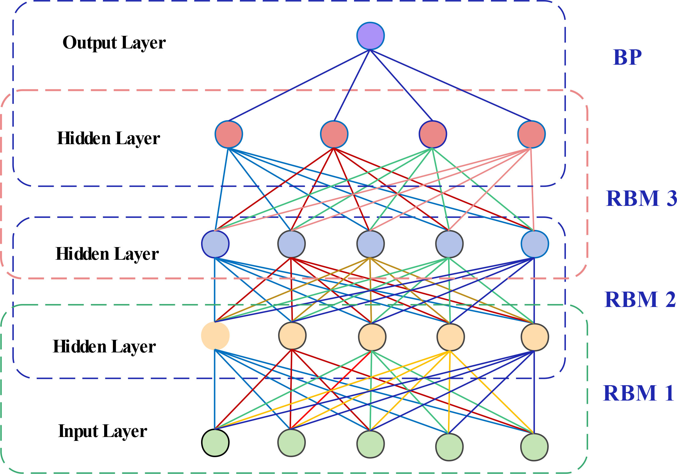
Figure 2 Structure diagram of the DBN model.
The optimization of the DBN model consists of two steps: unsupervised training and supervised fine-tuning. The DBN trains each layer of RBM separately, determines the weights and offsets of the first RBM, and uses the states of its hidden neurons as the input vector for the second RBM. After the second RBM is fully trained, the second RBM is stacked on top of the first RBM, and each layer of RMB is trained in turn, making sure to extract as much feature information as possible.
The last layer of the DBN is the BP neural network. During supervised tuning training, the BP algorithm is used to update the weights and biases of the model. Each layer of RBM can only ensure that the weights and bias values in its own layer are optimal for the feature vector mapping of this layer and not for the feature vector mapping of the entire DBN. The BP algorithm propagates the error information from top to bottom to each layer of the RBM and fine-tunes the entire DBN layer by layer. RBM is a shallow neural network with only two layers. The training time of RBM is significantly reduced compared with the deep neural network. The overall training of the DBN deep neural network is simplified to the training of multiple RBMs, which can improve the training efficiency and speed up the convergence speed. After training, the network is fine-tuned by the BP algorithm, so that the model converges to the local optimum, improves the convergence accuracy, and realizes the efficient training of the DBN neural network. The DBN prevents falling into a local optimum through unsupervised layer-by-layer training and improves the convergence speed and accuracy through supervised fine-tuning.
2.5 Evaluation of the predictive models
The accuracy of the prediction model is measured by calculating the similarity between the predicted value and the actual value. Common evaluation indicators include mean absolute error (MAE), mean absolute percentage error (MAPE), mean squared error (MSE), Willmott indexr (WI)(Willmott et al., 2012) and goodness of fit (). In this paper, the above indicators are used to evaluate the prediction performance of our model and other comparative models. Assuming that the predicted value is , the actual value is , and is the number of samples, the formulas of each indicator are as follows: (13), (14), (15), (16) and (17).
where is the mean of all samples.
3 Simulation experiment and result analysis
3.1 Decomposition of dissolved oxygen time series
Aquaculture water quality data are easily affected by the external environment, biological activities and fishermen intervention. They have the characteristics of nonlinearity and instability and are affected by the accuracy and performance of water quality sensor acquisition equipment, and the data contain much noise. Therefore, training the model directly with the original dissolved oxygen time series limits the accuracy and stability of the prediction to a certain extent. Through the mode decomposition of VMD, multiple IMF subsequences with different frequency scales and relative stability are obtained. Using each subsequence for model training can greatly improve the prediction accuracy.
When applying VMD for mode decomposition, we can set the number of mode decomposition components according to the data characteristics. When the number of modes is too small, some important information in the original signal will be filtered, which will affect the accuracy of subsequent predictions. When the number of modes is too large, the center frequencies of adjacent mode components will be closer, resulting in mode overlap and excessive decomposition. In this paper, when determining the number of VMD modes, the MAE of the original signal and the decomposed mode reconstruction sequence is used as the optimization index, and the mode decomposition number is determined according to the change trend of the MAE value. The calculation of the MAE is shown in Equation (18).
In the above formula, is the original signal to be decomposed, is the decomposed mode component, is the number of mode components, and is the length of the time series. The VMD of 8640 dissolved oxygen data from Weihai Demingmarine ranching from June 1, 2021, to August 1, 2021, is taken as an example to optimize the mode decomposition number. In this paper, the number of decomposition components is set in the range of 2 to 10. After each decomposition step, the decomposed IMF sequence is reconstructed, and the MAE value of the reconstructed sequence and the original sequence are calculated. From the variation trend of the MAE in Figure 3, it can be found that when the number of decomposition modes is 4, the value of the MAE tends to be stable, so the number of VMD modes of this dissolved oxygen time series is set to 4.
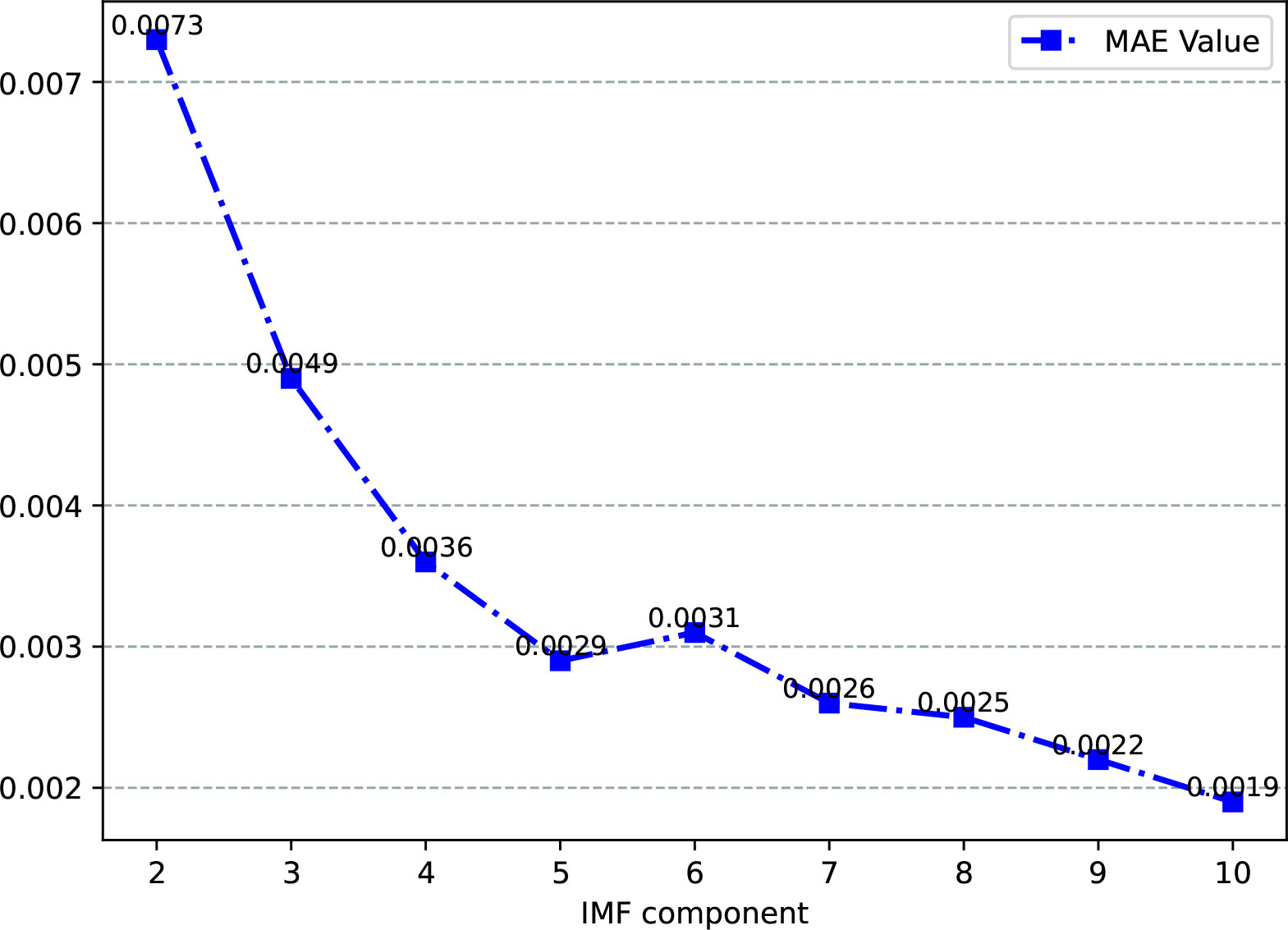
Figure 3 The change curve of the MAE value.
Figure 4 shows the decomposition effect of this dissolved oxygen time series.
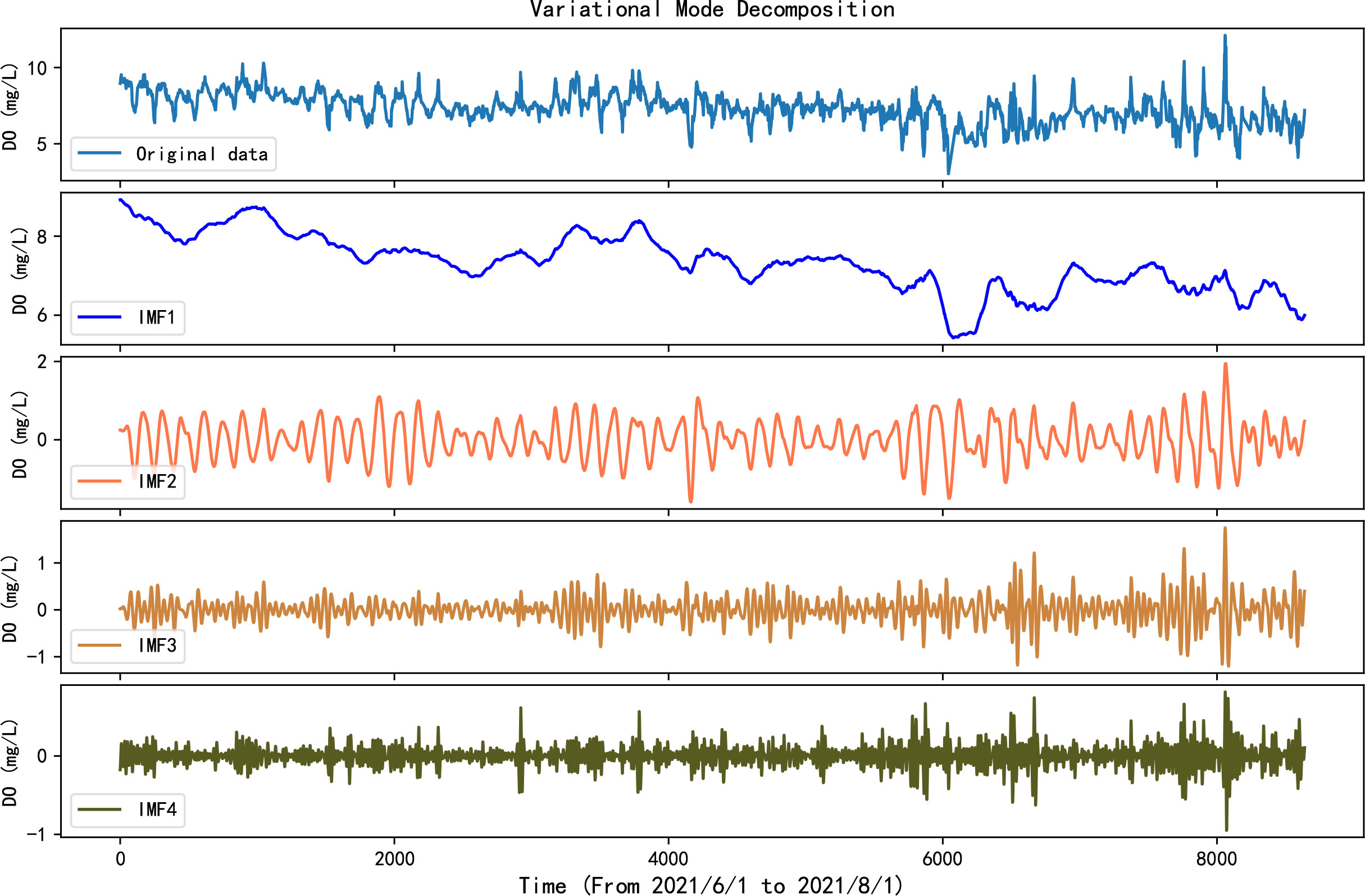
Figure 4 VMD of the dissolved oxygen time series.
3.2 Improved slime mould algorithm
The SMA has a simple structure and strong global search ability, but it also has shortcomings, such as a weak shrinkage mechanism and the tendency to easily fall into a local optimum. To make the SMA have better convergence accuracy and more stability, this paper uses elite opposition-based learning and a nonlinear convergence factor to improve it and proposes a multi strategy ISMA.
The opposition-based learning (OBL) model proposed by Tizhoosh calculates the current solution and the opposite solution in the process of searching for a feasible solution to a problem and selects an item that is closer to the optimal solution for the next iteration (Rahnamayan et al., 2008). OBL has been applied to improve various intelligent algorithms (Gupta et al., 2020; Shekhawat and Saxena, 2020; Tubishat et al., 2020; Wang et al., 2021; Li et al., 2022a).
Elite OBL (EOBL) forms an elite population and its opposite population based on the individual with the best fitness and then selects an individual with better fitness from the two populations to form a new population (Abualigah et al., 2021).
Assuming that at the t-th iteration, is the elite solution of individual in the dimension, then its opposite solution is . Its solution formula is shown in equation (19).
Among them, is a random value in the range of 0 to 1, and and are the minimum and maximum values of the j-th dimension individual, respectively. If the elite opposition solution exceeds the boundary, it is reset by random generation, as shown in formula (20).
The performance of the slime mould optimization algorithm is greatly affected by the quality of the initial population. A high-quality initial population can speed up the convergence of the algorithm and help to find the global optimal solution. This paper applies the EOBL strategy to the initialization of the SMA population, calculates the fitness value, obtains the elite slime mould individuals and dynamic boundaries, and improves the quality and diversity of the initial population.
In the iterative optimization process of SMA, the change in parameter has an important influence on balancing the global search ability and local exploration ability. Parameter decreases rapidly in the early iterations, this decrease slows down inthe later iterations, and a smaller in the early stage is not conducive to global exploration. Therefore, this paper proposes a new nonlinear decreasing strategy, and the updated formula for parameter is shown in (21).
Among them, is the current number of iterations, and is the maximum number of iterations.
As shown in Figure 5, the parameter a in this paper decreases slowly in the early stage, which is beneficial to global exploration. In later iterations, the speed of convergence is accelerated, which is beneficial to the local search.
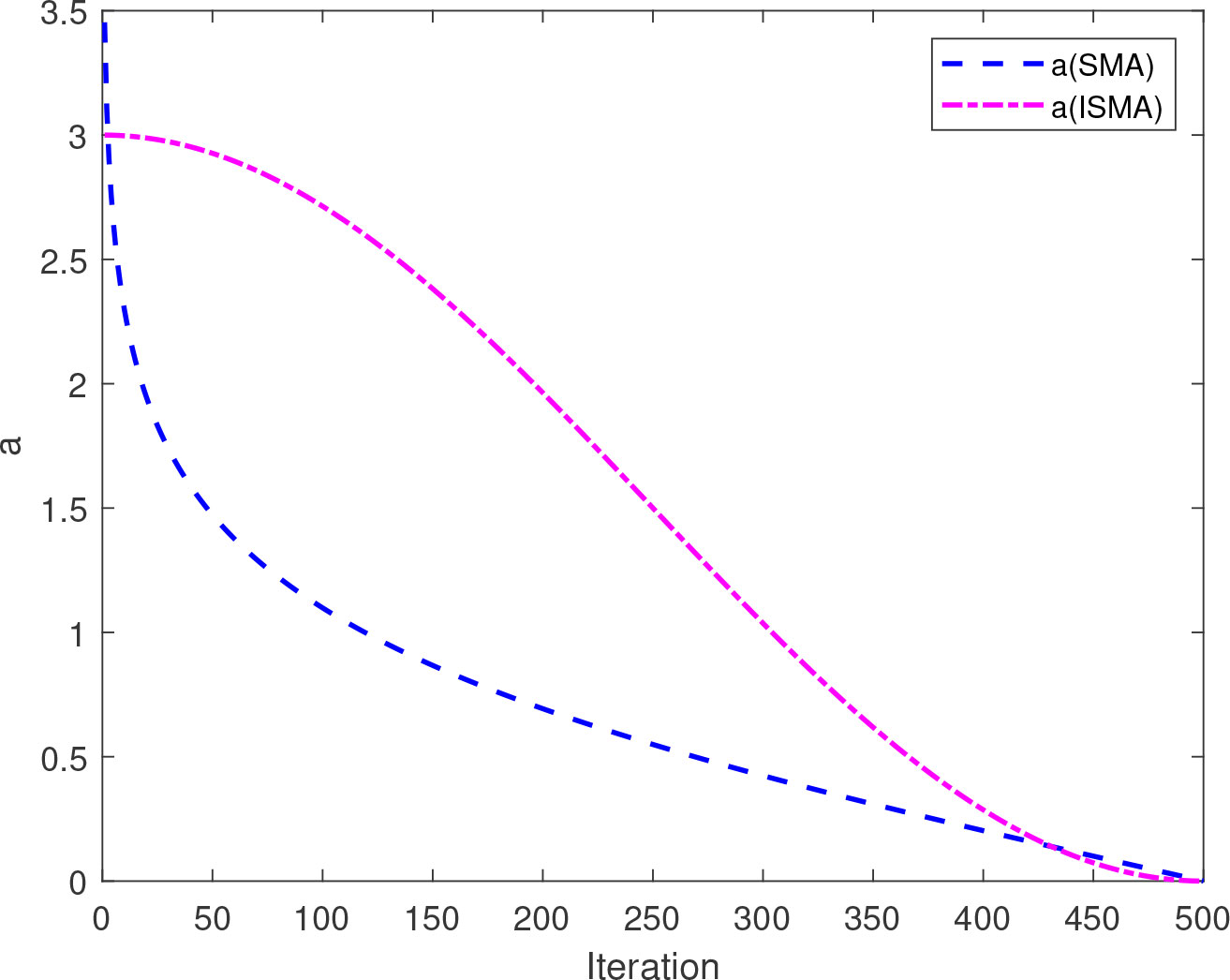
Figure 5 Convergence curve for parameter a.
3.3 DBN prediction model optimized based on the ISMA
In the construction of the DBN prediction model, several hyperparameter settings are involved, including the number of hidden layers, the number of nodes in each layer, the training times and learning rate in the unsupervised pretraining stage and the momentum. If the hyperparameter optimization is carried out by means of experimental verification, the process is slow, and it is difficult to obtain the best combination of hyperparameters. Therefore, this paper uses the ISMA to optimize the hyperparameters to build the prediction model.
The construction steps of an aquaculture water quality prediction model (VMD-ISMA-DBN) based on VMD and the ISMA to optimize the DBN are as follows.
(1) In view of the nonlinear and nonstationary characteristics of the dissolved oxygen series in aquaculture water quality, VMD was used to decompose the data series into multiple relatively stable IMF components.
(2) EOBL and a nonlinear convergence factor are applied to improve the optimization performance of the SMA to improve its convergence accuracy and stability.
(3) The optimization algorithm of DBN hyperparameters is studied, and a DBN prediction model optimized by the ISMA (ISMA-DBN) is constructed.
(4) Take each IMF subsequence decomposed by VMD as input samples to train the ISMA-DBN model, obtain the optimal hyperparameter combination of each sequence, and predict each subsequence.
(5) The prediction values of each IMF subsequence are superimposed to obtain the final prediction result of the original sequence, and the performance of the prediction model is verified by comparative experiments.
The structure diagram of the VMD-ISMA-DBN prediction model is shown in Figure 6.
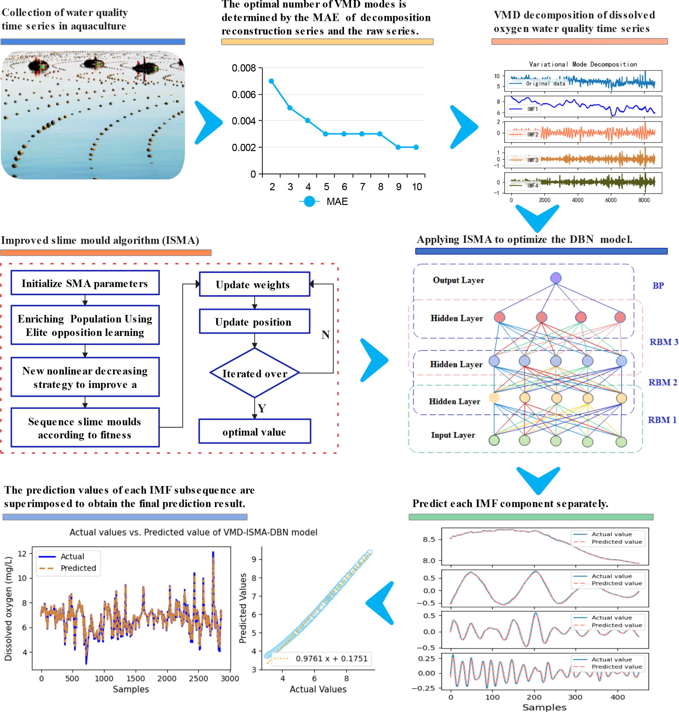
Figure 6 Framework of the VMD-ISMA-DBN prediction model.
Using the dissolved oxygen data of the Laizhou marine ranch as the experimental sample of the VMD-ISMA-DBN model, the four IMF subsequences obtained by mode decomposition were trained and predicted. The first 80% of the data were used as the training set, and the last 20% of the data were used as the test set. Figure 7 shows the convergence curves for each IMF sequence trained using the SMA-DBN model and the ISMA-DBN model respectively
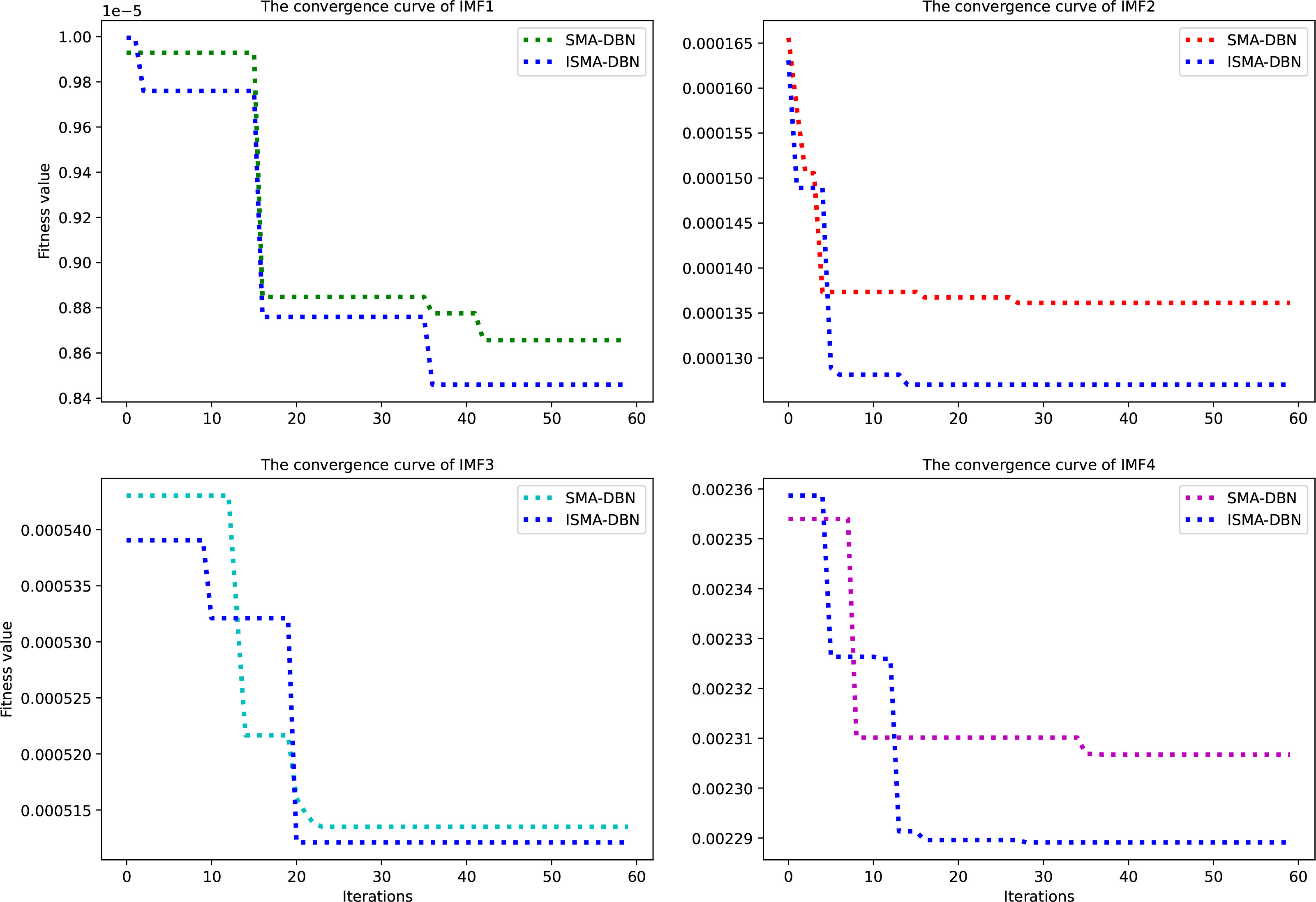
Figure 7 Convergence curves of the IMF components.
As shown in Figure 7, in the iterative optimization process of the four IMF subsequences, compared with SMA-DBN, ISMA-DBN has faster convergence speed, higher convergence accuracy, and stronger ability to avoid falling into local optimum. Table 2 shows the optimal values of the hyperparameters of the DBN model optimized by the ISMA for each IMF sequence, including the learning rate of the pretraining (lr_p), the number of iterations for pretraining (epo_p), the learning rate for fine-tuning (lr_f), the number of iterations for fine-tuning (epo_f), the momentum, the batch size (B_S) and the number of hidden layers (nlayer). From the data in Table 2, it can be seen that the prediction of the two high-frequency components of IMF3 and IMF4 is relatively difficult, and the network structure is more complex than the two low-frequency components of IMF1 and IMF2.
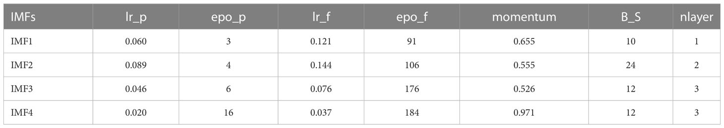
Table 2 Optimal hyperparameter values of the DBN for each IMF subsequence.
Figure 8 shows the fitting effect of each IMF subsequence predicted by the VMD-ISMA-DBN model proposed in this paper.
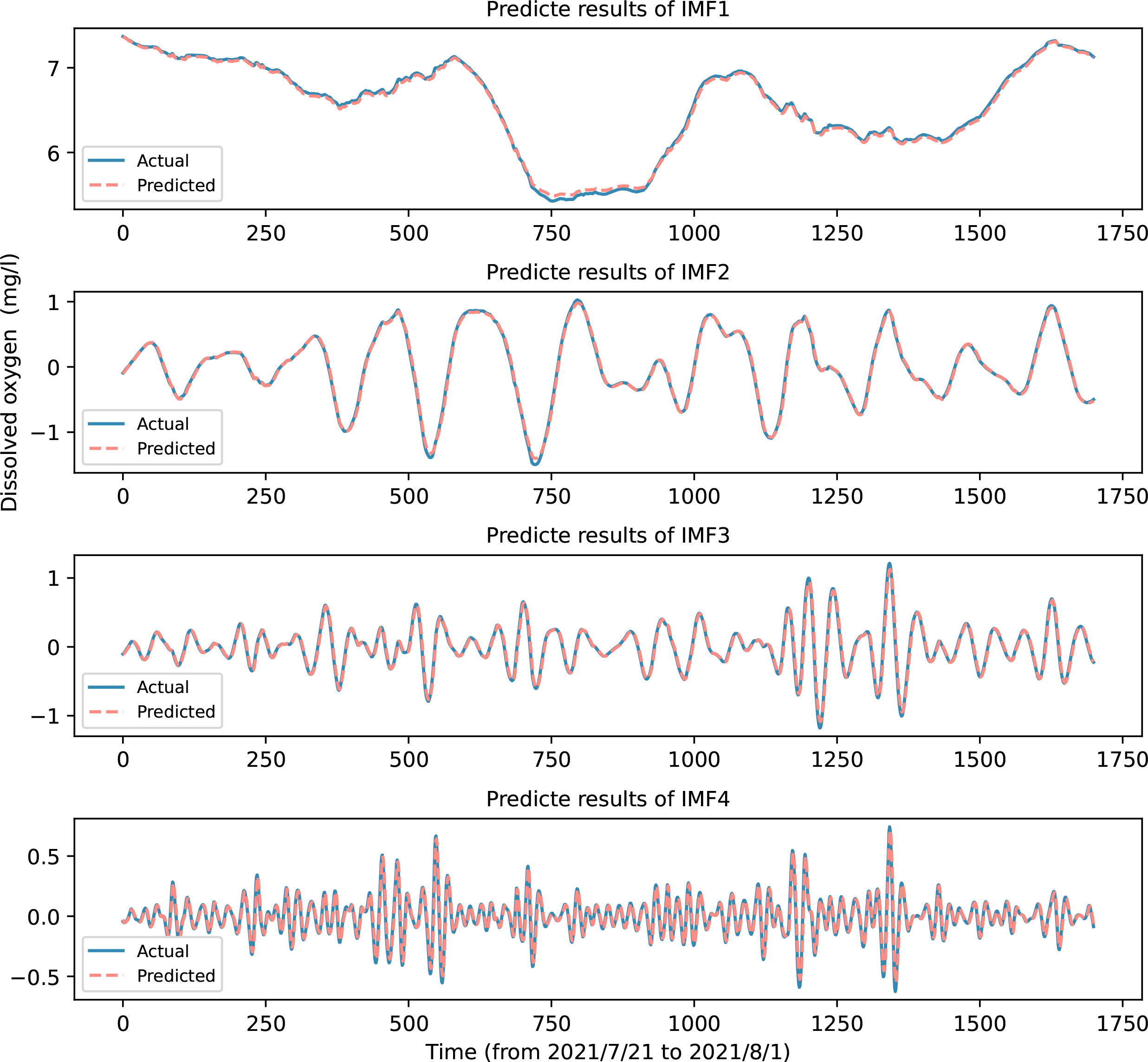
Figure 8 Prediction effect of the VMD-ISMA-DBN model on IMF subsequences.
Figure 8 shows that after dividing the original time series into relatively stable IMF subsequences, the complexity of the series is reduced, and the prediction accuracy is greatly improved. The low-frequency components with strong regularity and large amplitudes have an accurate prediction effect. There are some errors in the prediction of the high-frequency signal, but due to its small amplitude, it has little effect on the final prediction after being superimposed with the prediction result of the low-frequency component.
The prediction results of each IMF component are superimposed to obtain the final prediction results of the original dissolved oxygen time series. As shown in Figure 9, the predicted value after superposition fits well with the actual value, and the model in this paper shows very accurate prediction performance.
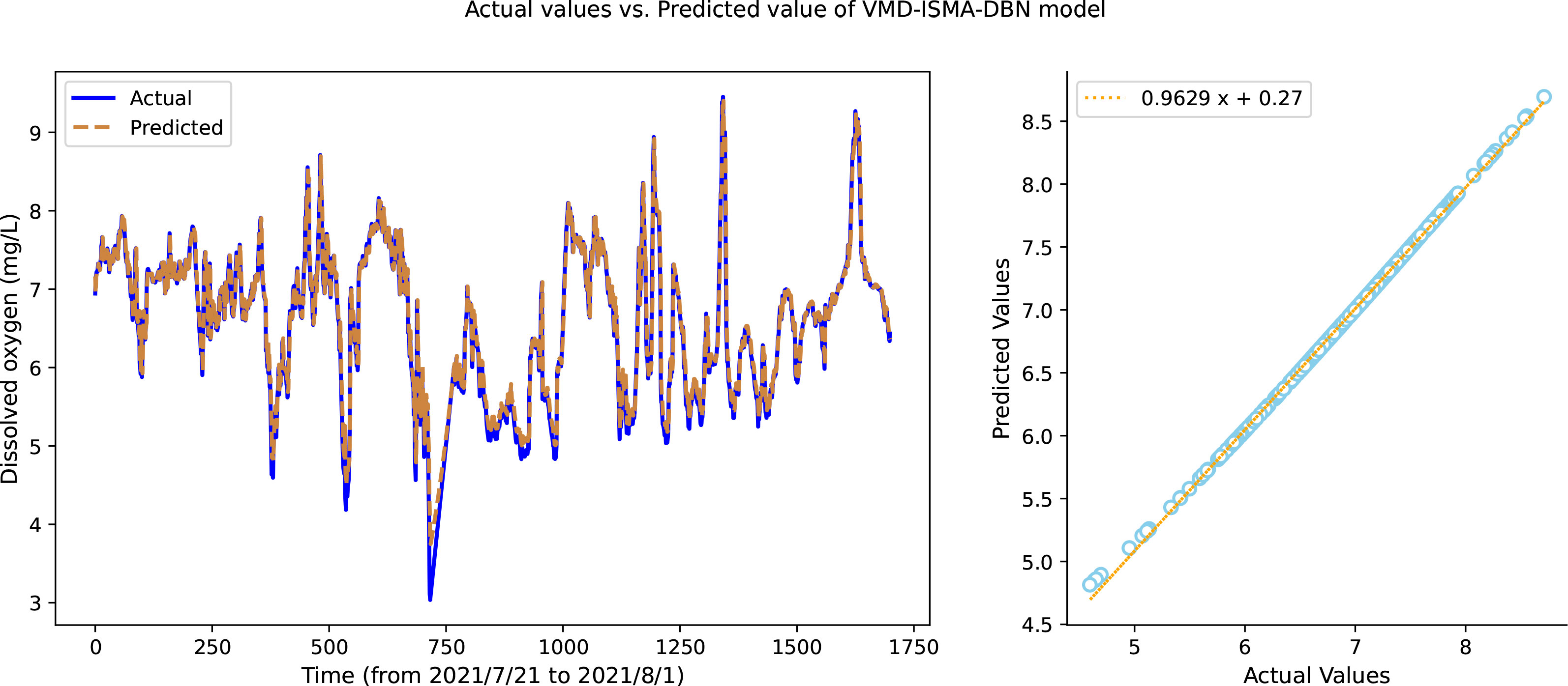
Figure 9 Final prediction effect of the VMD-ISMA-DBN model.
4 Results
4.1 Ablation study
To verify the effectiveness of each component of VMD-ISMA-DBN in improving model performance, the following five prediction models were constructed for ablation research.
(1) A DBN is used to build a prediction model, the hyperparameters of the model are .manually selected through experience, and the original dissolved oxygen sequence is used as the input sample.
(2) The SMA is used to optimize the DBN model, the model hyperparameters are selected through the optimization algorithm, the original dissolved oxygen sequence is used as the input sample, and the model is named SMA-DBN.
(3) Only the EOBL mechanism is used to improve the SMA; the improved algorithm is used to optimize the DBN model, the original dissolved oxygen sequence is used as the input sample, and the model is named ISMA1-DBN.
(4) The SMA is improved only by changing the convergence factor. The DBN model is optimized with the ISMA, the original dissolved oxygen sequence is used as the input sample, and the model is named ISMA2-DBN.
(5) The SMA is improved by using the combination of the EOBL mechanism and by changing the convergence factor, and the ISMA is used to optimize the DBN. The original sequence is used as the input sample, and the model is named ISMA-DBN.
The above five models are compared with the VMD-ISMA-DBN model proposed in this paper, and the experimental results are shown in Figure 10.

Figure 10 Results of the ablation experiments.
The evaluation index values of each experimental model are shown in Table 3.
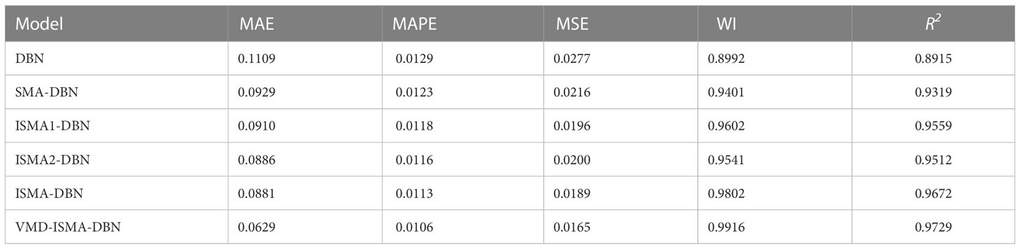
Table 3 The prediction performance evaluation index value of each model.
As shown in Figure 10 and Table 3, the DBN model needs to adjust many hyperparameters, and the prediction error is large if adjusted purely by experience. The training process of the DBN model is optimized by the SMA, the setting of hyperparameters is more reasonable, and the prediction error is reduced. The two strategies of EOBL and the improved convergence factor are separately used to optimize the SMA. The ISMA further optimizes the hyperparameter combination of the DBN, and the prediction accuracy is further improved. The original dissolved oxygen time series is preprocessed by VMD, and the decomposed signal is smoother, which can reduce the difficulty of prediction and significantly improve the prediction performance. The prediction curve of the VMD-ISMA-DBN model proposed in this paper has a better fitting effect than the other methods in the maximum value and minimum value, and the prediction trend is closer to the actual curve, which illustrates the more accurate prediction effect.
4.2 Comparative experiments
To further verify the prediction performance of the VMD-ISMA-DBN model, it is compared with six other intelligent prediction models, namely, the autoregressive integrated moving average model (ARIMA) (Xuan et al. (2021)), random forest (RF) regressor (Tiyasha et al. (2021)), temporal convolutional network (TCN) (Li et al. (2022b)), extreme learning machine (ELM) (An et al. (2022)), gated recurrent unit (GRU) (Cao et al. (2020) and long short-term memory (LSTM) (Barzegar et al. (2020)) The main parameters of each model are shown in Table 4.
Table 4 The main parameters of each comparative model.
Figure 11 shows the prediction effect of each comparative model and VMD-ISMA-DBN on a 12-hour dissolved oxygen time series. It shows that the VMD-ISMA-DBN model proposed in this paper has a better prediction effect on dissolved oxygen water quality data than the other comparison models, and the prediction curve is more in line with the actual time series.
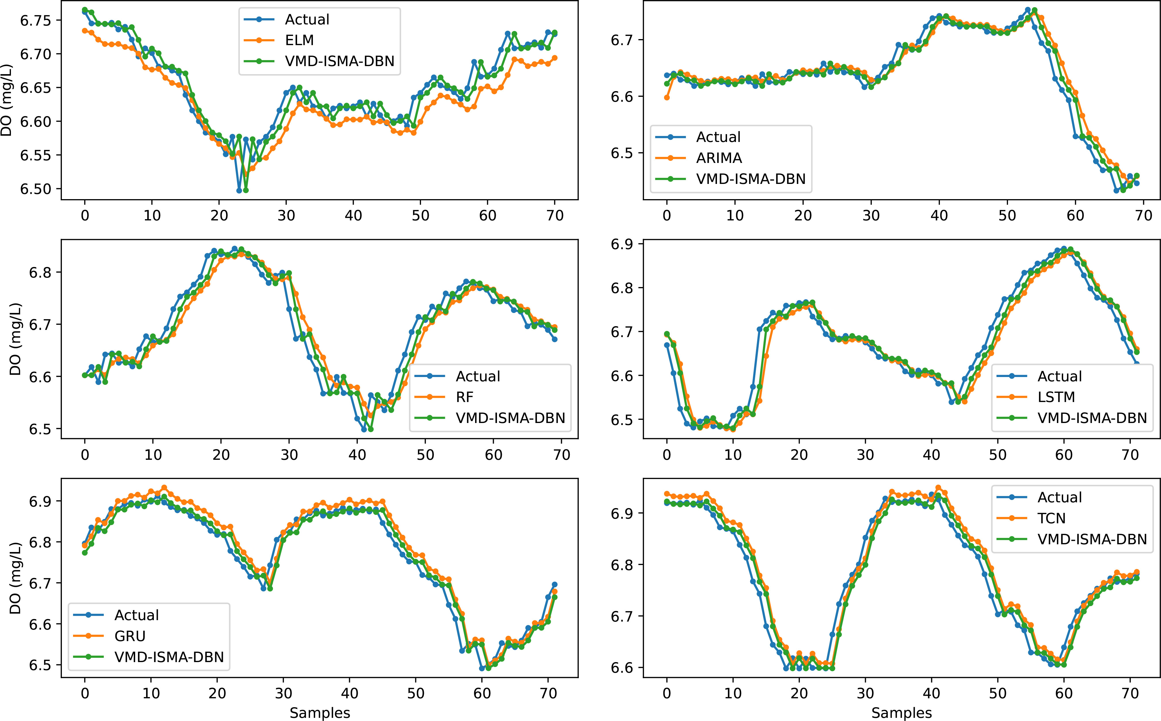
Figure 11 Comparison of the prediction effects of each model and VMD-ISMA-DBN.
The ARIMA model performs stationary preprocessing on nonstationary sequences by means of differencing, and it cannot capture nonlinear relationships well. For unstable and nonlinear water quality data, the hyperparameter optimization process is complicated, and the prediction accuracy is lower than that of other models. The RF regressor model integrates multiple decision trees, and overfitting may occur when it is used for the prediction of time series with considerable noise. Due to the complexity of its structure, it takes more time to train than other models. The ELM has the characteristics of few training parameters and a fast training speed. However, for aquaculture water quality data with noise interference, the prediction effect of the ELM model is unstable. The LSTM and GRU neural networks achieve good results in time series prediction and solve the long-term dependency problem of RNNs. The vanishing gradient problem may occur during the training process. The model structure of the LSTM and GRU models is relatively complex, and it is easy to consume much memory when the training sequence is long. The TCN prediction model has the advantages of a stable gradient, low training memory requirements and accepting variable length inputs. The TCN model achieves better performance than the LSTM and GRU models in the prediction of dissolved oxygen time series. The DBN has the advantages of easy expansion, fast training, and less convergence time. In this paper, the improved SMA is used to optimize the hyperparameters of the DBN, and VMD is used to decompose the dissolved oxygen time series. The model in this paper achieves higher prediction accuracy than the other comparative models.
To verify the generalization performance of the model in this paper, the dissolved oxygen data of 6 other marine ranches were selected for experimental verification, and different time spans were selected to study the short-term and long-term prediction performance of the model. The water quality data of all marine ranches were collected every 10 minutes, and approximately 140 pieces of effective dissolved oxygen data were collected every day. During the experiment, 80% of the data are selected as the training set, and 20% of the data are used as the test set. Table 5 shows the statistics of the experimental data.
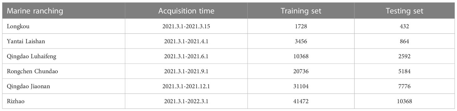
Table 5 Statistics of the experimental data.
Figure 12 shows that the model in this paper achieves good prediction performance for the dissolved oxygen time series from the six marine ranches, and the prediction curve fits the actual data curve well, indicating that the prediction model has strong generalization performance and stability. Observing the prediction effect of different time spans from 15 days to 1 year, the prediction error of the long-term series increases to a certain extent, and the fitting effect of the data mutation decreases. The reason for this phenomenon may be the accumulation of prediction errors. The model in this paper eliminates the influence of data non stationarity on the prediction effect by decomposing the water quality data by VMD and optimizes the parameters of the DBN model through the ISMA, which makes the hyperparameter settings reasonable and improves the prediction accuracy. The experimental results show that the VMD-ISMA-DBN model proposed in this paper is suitable for the prediction of aquaculture water quality time series.
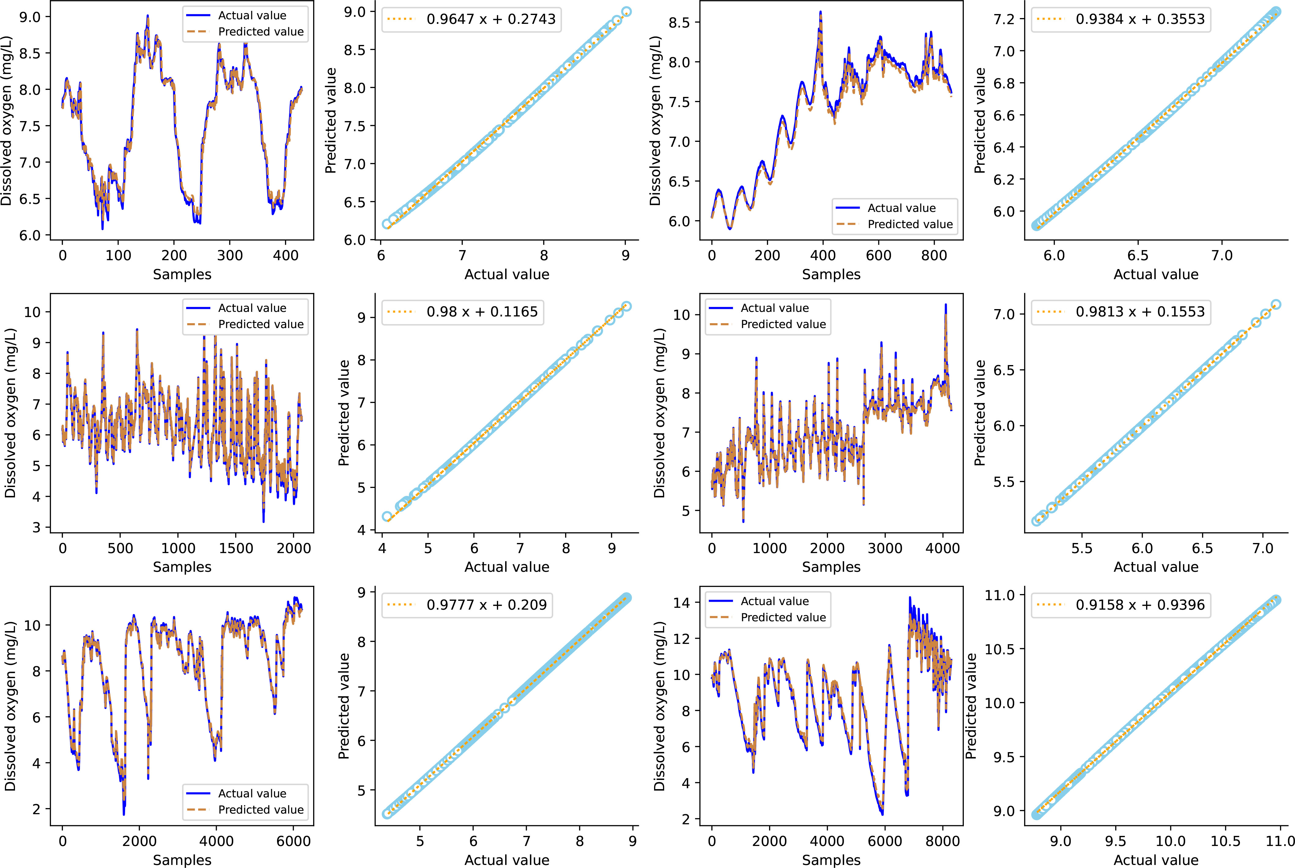
Figure 12 Prediction effect of the VMD-ISMA-DBN model on water quality data from multiple marine ranches.
5 Conclusion
In order to accurately predict the change trend of dissolved oxygen time series in aquaculture water, this paper proposes a DBN model based on ISMA optimization, and uses the VMD algorithm to decompose the input samples to reduce the impact of data fluctuations on water quality prediction. Ablation study shows that this model can significantly improve the prediction performance of the stand-alone DBN model. Comparative experiments show that this model has higher prediction accuracy and better generalization performance than other commonly used intelligent prediction models.
In this paper, a univariate recursive forecasting method is used to establish a model, and the historical time series of dissolved oxygen is used to predict future values. This model does not consider the impact of environmental factors and other water quality indicators on dissolved oxygen, which limits the universality of the prediction model to a certain extent.
In the future, we will study the interaction between the spatiotemporal environment and water quality indicators, build a multivariate water quality prediction model, and study the optimization of the hyperparameters of the deep learning model by intelligent algorithms to further improve the prediction accuracy.
Data availability statement
The original contributions presented in the study are included in the article/Supplementary material. Further inquiries can be directed to the corresponding authors.
Author contributions
HY conceived the framework of the paper, designed simulation experiments and intelligent algorithms, and co-wrote the paper. MS collected experimental data, designed figures and tables, conducted paper reviewing, and performed critical corrections. SL analyzed the experimental data, conducted simulated experiments and algorithm design, and co-wrote the paper.
Conflict of interest
The authors declare that the research was conducted in the absence of any commercial or financial relationships that could be construed as a potential conflict of interest.
Publisher’s note
All claims expressed in this article are solely those of the authors and do not necessarily represent those of their affiliated organizations, or those of the publisher, the editors and the reviewers. Any product that may be evaluated in this article, or claim that may be made by its manufacturer, is not guaranteed or endorsed by the publisher.
References
Abualigah L., Diabat A., Elaziz M. A. (2021). Improved slime mould algorithm by opposition-based learning and levy flight distribution for global optimization and advances in real-world engineering problems. J. Ambient Intell. Human. Comput. 14, 1163–1202 doi: 10.1007/s12652-021-03372-w
Ahmadianfar I., Bozorg-Haddad O., Chu X. (2020). Gradient-based optimizer: a new metaheuristic optimization algorithm. Inf. Sci. 540, 131–159. doi: 10.1016/j.ins.2020.06.037
Ahmadianfar I., Heidari A. A., Noshadian S., Chen H., Gandomi A. H. (2022). Info: an efficient optimization algorithm based on weighted mean of vectors. Expert Syst. Appl. 195, 116516. doi: 10.1016/j.eswa.2022.116516
Alsattar H. A., Zaidan A. A., Zaidan B. B. (2020). Novel meta-heuristic bald eagle search optimisation algorithm. Artif. Intell. Rev. 53, 2237–2264. doi: 10.1007/s10462-019-09732-5
An G., Chen L., Tan J., Jiang Z., Li Z., Sun H. (2022). Ultra-short-term wind power prediction based on pvmd-esma-delm. Energy Rep. 8, 8574–8588. doi: 10.1016/j.egyr.2022.06.079
Antanasijević D., Pocajt V., Perić-Grujić A., Ristić M. (2014). Modelling of dissolved oxygen in the danube river using artificial neural networks and monte carlo simulation uncertainty analysis. J. Hydrol. 519, 1895–1907. doi: 10.1016/j.jhydrol.2014.10.009
Areerachakul S., Sophatsathit P., Lursinsap C. (2013). Integration of unsupervised and supervised neural networks to predict dissolved oxygen concentration in canals. Ecol. Model. 261-262, 1–7. doi: 10.1016/j.ecolmodel.2013.04.002
Barzegar R., Aalami M. T., Adamowski J. (2020). Short-term water quality variable prediction using a hybrid cnn–lstm deep learning model. Stochastic Environ. Res. Risk Assess. 34, 415–433. doi: 10.1007/s00477-020-01776-2
Bi J., Zhang L., Yuan H., Zhang J. (2023). Multi-indicator water quality prediction with attention-assisted bidirectional lstm and encoder-decoder. Inf. Sci. 625, 65–80 doi: 10.1016/j.ins.2022.12.091
Brooks W., Corsi S., Fienen M., Carvin R. (2016). Predicting recreational water quality advisories: a comparison of statistical methods. Environ. Model. Software 76, 81–94. doi: 10.1016/j.envsoft.2015.10.012
Cao X., Liu Y., Wang J., Liu C., Duan Q. (2020). Prediction of dissolved oxygen in pond culture water based on k-means clustering and gated recurrent unit neural network. Aquacul. Eng. 91, 102122. doi: 10.1016/j.aquaeng.2020.102122
Chen Z., Hu Z., Xu L., Zhao Y., Zhou X. (2022). Da-bi-sru for water quality prediction in smart mariculture. Comput. Electron. Agric. 200, 107219. doi: 10.1016/j.compag.2022.107219
Dragomiretskiy K., Zosso D. (2014). Variational mode decomposition. IEEE Trans. Signal Process. 62, 531–544. doi: 10.1109/TSP.2013.2288675
Emam M. M., Houssein E. H., Ghoniem R. M. (2023). A modified reptile search algorithm for global optimization and image segmentation: case study brain mri images. Comput. Biol. Med. 152, 106404. doi: 10.1016/j.compbiomed.2022.106404
Gupta S., Deep K., Heidari A. A., Moayedi H., Wang M. (2020). Opposition-based learning harris hawks optimization with advanced transition rules: principles and analysis. Expert Syst. Appl. 158, 113510. doi: 10.1016/j.eswa.2020.113510
Hassan M. M., Alam M. G. R., Uddin M. Z., Huda S., Almogren A., Fortino G. (2019). Human emotion recognition using deep belief network architecture. Inf. Fusion 51, 10–18. doi: 10.1016/j.inffus.2018.10.009
Heidari A. A., Mirjalili S., Faris H., Aljarah I., Mafarja M., Chen H. (2019). Harris Hawks optimization: algorithm and applications. Future Generat. Comput. Syst. 97, 849–872. doi: 10.1016/j.future.2019.02.028
Hinton G. E., Osindero S., Teh Y.-W. (2006). A fast learning algorithm for deep belief nets. Neural Comput. 18, 1527–1554. doi: 10.1162/neco.2006.18.7.1527
Hinton G. E., Salakhutdinov R. R. (2006). Reducing the dimensionality of data with neural networks. Science 313, 504–507. doi: 10.1126/science.1127647
Hu G., Zhong J., Wang X., Wei G. (2022). Multi-strategy assisted chaotic coot-inspired optimization algorithm for medical feature selection: a cervical cancer behavior risk study. Comput. Biol. Med. 151, 106239. doi: 10.1016/j.compbiomed.2022.106239
Huan J., Cao W., Qin Y. (2018). Prediction of dissolved oxygen in aquaculture based on eemd and lssvm optimized by the bayesian evidence framework. Comput. Electron. Agric. 150, 257–265. doi: 10.1016/j.compag.2018.04.022
Huang J., Huang Y., Hassan S. G., Xu L., Liu S. (2021). Dissolved oxygen content interval prediction based on auto regression recurrent neural network. J. Ambient Intell. Human. Comput. 14, 7255–7264. doi: 10.1007/s12652-021-03579-x
Jafari H., Rajaee T., Kisi O. (2020). Improved water quality prediction with hybrid wavelet-genetic programming model and shannon entropy. Natural Resour. Res. 29, 3819–3840. doi: 10.1007/s11053-020-09702-7
Jiang M., Liang Y., Feng X., Fan X., Pei Z., Xue Y., et al. (2018). Text classification based on deep belief network and softmax regression. Neural Comput. Appl. 29, 61–70. doi: 10.1007/s00521-016-2401-x
Khatami A., Khosravi A., Nguyen T., Lim C. P., Nahavandi S. (2017). Medical image analysis using wavelet transform and deep belief networks. Expert Syst. Appl. 86, 190–198. doi: 10.1016/j.eswa.2017.05.073
Kisi O., Alizamir M., Docheshmeh Gorgij A. (2020). Dissolved oxygen prediction using a new ensemble method. Environ. Sci. pollut. Res. 27, 9589–9603. doi: 10.1007/s11356-019-07574-w
Kuremoto T., Kimura S., Kobayashi K., Obayashi M. (2014). Time series forecasting using a deep belief network with restricted boltzmann machines. Neurocomputing 137, 47–56. doi: 10.1016/j.neucom.2013.03.047
Li S., Chen H., Wang M., Heidari A. A., Mirjalili S. (2020). Slime mould algorithm: a new method for stochastic optimization. Future Generat. Comput. Syst. 111, 300–323. doi: 10.1016/j.future.2020.03.055
Li C., Li Z., Wu J., Zhu L., Yue J. (2018). A hybrid model for dissolved oxygen prediction in aquaculture based on multi-scale features. Inf. Process. Agric. 5, 11–20. doi: 10.1016/j.inpa.2017.11.002
Li W., Wei Y., An D., Jiao Y., Wei Q. (2022b). Lstm-tcn: dissolved oxygen prediction in aquaculture, based on combined model of long short-term memory network and temporal convolutional network. Environ. Sci. pollut. Res. 29, 39545–39556. doi: 10.1007/s11356-022-18914-8
Li M., Xu G., Lai Q., Chen J. (2022a). A chaotic strategy-based quadratic opposition-based learning adaptive variable-speed whale optimization algorithm. Math. Comput. Simulation 193, 71–99. doi: 10.1016/j.matcom.2021.10.003
Liu S., Xu L., Li D. (2016). Multi-scale prediction of water temperature using empirical mode decomposition with back-propagation neural networks. Comput. Electrical Eng. 49, 1–8. doi: 10.1016/j.compeleceng.2015.10.003
Lu H., Ma X. (2020). Hybrid decision tree-based machine learning models for short-term water quality prediction. Chemosphere 249, 126169. doi: 10.1016/j.chemosphere.2020.126169
Mirjalili S., Lewis A. (2016). The whale optimization algorithm. Adv. Eng. Software 95, 51–67. doi: 10.1016/j.advengsoft.2016.01.008
Naruei I., Keynia F. (2021). Wild horse optimizer: a new meta-heuristic algorithm for solving engineering optimization problems. Eng. Comput. 38, 3025–3056. doi: 10.1007/s00366-021-01438-z
Niu H., Xu K., Wang W. (2020). A hybrid stock price index forecasting model based on variational mode decomposition and lstm network. Appl. Intell. 50, 4296–4309. doi: 10.1016/j.compag.2019
Peraza-Vázquez H., Peña-Delgado A. F., Echavarría-Castillo G., Morales-Cepeda A. B., Velasco-Álvarez J., Ruiz-Perez F. (2021). A bio-inspired method for engineering design optimization inspired by dingoes hunting strategies. Math. Problem. Eng. 2021, 9107547. doi: 10.1155/2021/9107547
Pipelzadeh S., Mastouri R. (2021). Modeling of contaminant concentration using the classification-based model integrated with data preprocessing algorithms. J. Hydroinformat. 23, 639–654. doi: 10.2166/hydro.2021.138
Rahnamayan S., Tizhoosh H. R., Salama M. M. A. (2008). Opposition-based differential evolution. IEEE Trans. Evolution. Comput. 12, 64–79. doi: 10.1109/TEVC.2007.894200
Rajaee T., Khani S., Ravansalar M. (2020). Artificial intelligence-based single and hybrid models for prediction of water quality in rivers: a review. Chemomet. Intelligent Lab. Syst. 200, 103978. doi: 10.1016/j.chemolab.2020.103978
Rashedi E., Nezamabadi-pour H., Saryazdi S. (2009). Gsa: a gravitational search algorithm. Inf. Sci. 179, 2232–2248. doi: 10.1016/j.ins.2009.03.004
Ren Q., Wang X., Li W., Wei Y., An D. (2020). Research of dissolved oxygen prediction in recirculating aquaculture systems based on deep belief network. Aquacul. Eng. 90, 102085. doi: 10.1016/j.aquaeng.2020.102085
Ren Q., Zhang L., Wei Y., Li D. (2018). A method for predicting dissolved oxygen in aquaculture water in an aquaponics system. Comput. Electron. Agric. 151, 384–391. doi: 10.1016/j.compag.2018.06.013
Rozario A. P. R., Devarajan N. (2021). Monitoring the quality of water in shrimp ponds and forecasting of dissolved oxygen using fuzzy c means clustering based radial basis function neural networks. J. Ambient Intell. Human. Comput. 12, 4855–4862. doi: 10.1007/s12652-020-01900-8
Shekhawat S., Saxena A. (2020). Development and applications of an intelligent crow search algorithm based on opposition based learning. ISA Trans. 99, 210–230. doi: 10.1016/j.isatra.2019.09.004
Ta X., Wei Y. (2018). Research on a dissolved oxygen prediction method for recirculating aquaculture systems based on a convolution neural network. Comput. Electron. Agric. 145, 302–310. doi: 10.1016/j.compag.2017.12.037
Tiyasha T., Tung T. M., Bhagat S. K., Tan M. L., Jawad A. H., Mohtar W. H. M. W., et al. (2021). Functionalization of remote sensing and on-site data for simulating surface water dissolved oxygen: development of hybrid tree-based artificial intelligence models. Mar. pollut. Bull. 170, 112639. doi: 10.1016/j.marpolbul.2021.112639
Tubishat M., Idris N., Shuib L., Abushariah M. A., Mirjalili S. (2020). Improved salp swarm algorithm based on opposition based learning and novel local search algorithm for feature selection. Expert Syst. Appl. 145, 113122. doi: 10.1016/j.eswa.2019.113122
Wang G.-G., Deb S., Cui Z. (2019). Monarch butterfly optimization. Neural Comput. Appl. 31, 1995–2014. doi: 10.1007/s00521-015-1923-y
Wang G., Guo S., Han L., Song X., Zhao Y. (2022). Research on multi-modal autonomous diagnosis algorithm of covid-19 based on whale optimized support vector machine and improved d-s evidence fusion. Comput. Biol. Med. 150, 106181. doi: 10.1016/j.compbiomed.2022.106181
Wang S., Liu Q., Liu Y., Jia H., Abualigah L., Zheng R., et al. (2021). A hybrid ssa and sma with mutation opposition-based learning for constrained engineering problems. Comput. Intell. Neurosci. 2021, 6379469. doi: 10.1155/2021/6379469
Willmott C. J., Robeson S. M., Matsuura K. (2012). A refined index of model performance. Int. J. Climatol. 32, 2088–2094. doi: 10.1002/joc.2419
Xuan W., Tian W., Liao Z. (2021). Statistical comparison between sarima and ann’s performance for surface water quality time series prediction. Environ. Sci. pollut. Res. 28, 33531–33544. doi: 10.1007/s11356-021-13086-3
Xue J., Shen B. (2020). A novel swarm intelligence optimization approach: sparrow search algorithm. Syst. Sci. Control Eng. 8, 22–34. doi: 10.1080/21642583.2019.1708830
Yang Y., Chen H., Heidari A. A., Gandomi A. H. (2021). Hunger games search: visions, conception, implementation, deep analysis, perspectives, and towards performance shifts. Expert Syst. Appl. 177, 114864. doi: 10.1016/j.eswa.2021.114864
Yang H., Liu S. (2022). Water quality prediction in sea cucumber farming based on a gru neural network optimized by an improved whale optimization algorithm. PeerJ Comput. Sci. 8, 1000. doi: 10.7717/peerj-cs.1000
Zhang S., Wu J., Jia Y., Wang Y.-G., Zhang Y., Duan Q. (2021). A temporal lasso regression model for the emergency forecasting of the suspended sediment concentrations in coastal oceans: accuracy and interpretability. Eng. Appl. Artif. Intell. 100, 104206. doi: 10.1016/j.engappai.2021.104206
Zhang S., Wu J., Wang Y.-G., Jeng D.-S., Li G. (2022). A physics-informed statistical learning framework for forecasting local suspended sediment concentrations in marine environment. Water Res. 218, 118518. doi: 10.1016/j.watres.2022.118518
Zhao W., Wang L., Zhang Z. (2019). Atom search optimization and its application to solve a hydrogeologic parameter estimation problem. Knowledge-Based Syst. 163, 283–304. doi: 10.1016/j.knosys.2018.08.030
Keywords: dissolved oxygen, aquaculture, water quality prediction, variational mode decomposition, deep belief network, slime mould algorithm
Citation: Yang H, Sun M and Liu S (2023) A hybrid intelligence model for predicting dissolved oxygen in aquaculture water. Front. Mar. Sci. 10:1126556. doi: 10.3389/fmars.2023.1126556
Received: 18 December 2022; Accepted: 17 May 2023;
Published: 06 June 2023.
Edited by:
Shengyan Pu, Chengdu University of Technology, ChinaReviewed by:
Saad Shauket Sammen, University of Diyala, IraqJinran Wu, Australian Catholic University, Australia
Salim Heddam, University of Skikda, Algeria
Huiling Chen, Wenzhou University, China
Yonggang Li, Central South University, China
Copyright © 2023 Yang, Sun and Liu. This is an open-access article distributed under the terms of the Creative Commons Attribution License (CC BY). The use, distribution or reproduction in other forums is permitted, provided the original author(s) and the copyright owner(s) are credited and that the original publication in this journal is cited, in accordance with accepted academic practice. No use, distribution or reproduction is permitted which does not comply with these terms.
*Correspondence: Shue Liu, bHNlMzJAYnptYy5lZHUuY24=; Huanhai Yang, MjAxNTExODA5QHNkdGJ1LmVkdS5jbg==