Ensemble-based data assimilation for predictable zones and application for non-linear deep-water waves

The ensemble-based variational method is easier to implement and parallelize than the adjoint method. For circumstances in which observed data are too limited and sparse for oceanographic data assimilation, the surface wave reconstruction by ensemble adjoint-free data assimilation (SWEAD) method was developed in a previous study. SWEAD generates ensembles of search directions from Fourier modes to numerically differentiate the squared error between observed data and a physical model. However, Fourier modes are global bases and could be redundant for a narrow predictable zone confined by a dispersion relationship. To concentrate ensembles on the predictable zone, we propose using singular value decomposition (SVD) of the approximated Jacobian of the squared error. Here, the Jacobian was first approximated by the linear dispersion relationship and successively updated to consider the non-linearity of the physical system. A new criterion for reusing the ensemble was also devised for this new method, increasing the dimension of search directions. A twin experiment was conducted for non-linear deep-water waves, and the optimization efficiency of the new method—SWEAD using SVD (SWEAD-S)—was significantly greater than that of SWEAD. Expansion of the predictable zone caused by the effect of non-linearity on the wave group velocity is thought to be essential for this improvement.

1 Introduction

Observed ocean data are often spatially sparse, and the unobserved physical state needs to be estimated from the observed data for a certain period. The four-dimensional variational (4DVar) method estimates the physical state by minimizing the squared error between the value estimated by the physical model and the observed data as a cost function. To solve this least-squares problem, the linear approximation of the cost function must be determined. Methods to do this include the adjoint method, which uses the adjoint code of the physical model, and the ensemble method, which numerically differentiates the cost function by perturbed ensemble simulation. In recent years, the 4DVar method has been studied using the ensemble method because it does not require adjoint codes, which are expensive to implement, and because parallel computation is straightforward.

The ensemble-based 4DVar (En4DVAR) method utilizes the ensemble members of meteorological forecasts (Liu et al., 2008; Liu et al., 2009). The maximum likelihood ensemble filter (Zupanski, 2005) provides perturbed ensemble members from the square root decomposition of the error covariance matrix. The adjoint-free 4DVar (a4dVar) method alternates perturbation vectors in each iteration of the optimization process (Yaremchuk et al., 2009). The ensemble members are taken from the empirical orthogonal function (EOF) of the model trajectories (Panteleev et al., 2015) or the misfit derived from the model and observed data (Yaremchuk et al., 2016; Yaremchuk et al., 2017). In contrast to meteorological forecasts, a4dVar is generally suitable for oceanographic problems, given that there is no reliable information on their perturbation modes, which have a faster growth rate. a4dVar stacks the perturbed ensemble simulation to construct an approximate of the Hessian matrix of the cost function for efficient optimization. Similar to the Krylov subspace method, a4dVar reinitializes the perturbed ensemble simulation at certain conditions defined for the decay rate of the cost function (Yaremchuk et al., 2016) or the eigenvalues of the Hessian matrix (Yaremchuk et al., 2017).

Fujimoto and Waseda (2020) modified a4dVar and named their modified version SWEAD (surface wave reconstruction by ensemble adjoint-free data assimilation). SWEAD stacks the perturbed ensemble simulation to approximate the Hessian matrix while ensuring conformity to the linear approximation. Eventually, the dimension of the Hessian matrix has no limitations owing to the reinitialization, thereby increasing convergence speed. SWEAD was originally developed to estimate non-linear deep-water waves from observed data and has already been applied to field measurements in the ocean. SWEAD has been used to reconstruct a wave field around an observational tower with stereo camera data (Watanabe et al., 2019), and a non-linear wave group, called the oblique soliton, was captured (Waseda et al., 2021).

In dispersive waves such as deep-water waves, Wu (2004) and Qi et al. (2018) showed that the dispersion relationship confines the predictable zone for a limited amount of observational data. Meanwhile, SWEAD uses Fourier modes to generate perturbed ensembles (see Figure 2 of Fujimoto and Waseda (2020)), which are global bases and would be redundant for the limited predictable zone. Wu (2004) also showed the SVD analysis yields modes that are most sensitive to the cost function. The predictable zone can be evaluated by singular value decomposition (SVD) of the linear dispersion relationship (see Section 2.3.1). To improve optimization efficiency, we proposed using SVD to concentrate ensembles on the predictable zone and accumulate the generated ensembles. Several new techniques for efficient optimization were also devised. We name the method proposed in this study SWEAD-S (SWEAD utilizing SVD).

Section 2 reviews the ensemble methods, including SWEAD, and describes SWEAD-S. A typical example of non-linear dispersive waves is deep-water waves. This study targeted non-linear deep-water waves to demonstrate the performance of SWEAD-S. Section 3 provides a brief background of non-linear deep-water wave studies and the configuration of twin experiments. In Section 4, the performance of SWEAD and SWEAD-S are compared through twin experiments. Finally, Section 5 outlines the findings and directions for future research.

2 Methodology

The 4DVar method minimizes the squared error between a model prediction and observed data as the cost function as:

$\begin{array}{ll}L(\widetilde{\mathbf{\text{x}}})=\frac{1}{2}{(\widetilde{\mathit{\text{A}}}(\widetilde{\mathbf{\text{x}}})-\widetilde{\mathbf{\text{y}}})}^{*}{\mathbf{\text{R}}}^{-1}(\widetilde{\mathit{\text{A}}}(\widetilde{\mathbf{\text{x}}})-\tilde{\mathbf{y}})+\frac{1}{2}{\widetilde{\mathbf{\text{x}}}}^{*}{\mathbf{\text{D}}}^{-1}\tilde{\mathbf{x}},& (1)\end{array}$

where $\widetilde{\mathit{\text{A}}}(\widetilde{\mathbf{\text{x}}})$ is the prediction by the physical model, $\widetilde{\mathbf{\text{x}}}$ is the initial condition, $\widetilde{\mathbf{\text{y}}}$ is the observed data, and R and D are the observational and background error covariance matrices, respectively. To simplify the equation, the variables are scaled as:

$\begin{array}{ll}\mathbf{\text{x}}={\mathbf{\text{D}}}^{-1/2}\widetilde{\mathbf{\text{x}}},\mathbf{\text{y}}={\mathbf{\text{R}}}^{-1/2}\widetilde{\mathbf{\text{y}}},\mathit{\text{A}}(\mathbf{x})={\mathbf{\text{R}}}^{-1/2}\widetilde{\mathit{\text{A}}}(\widetilde{\mathbf{\text{x}}}).& (2)\end{array}$

The cost function can be reduced to:

$\begin{array}{ll}L(\mathbf{\text{x}})=\frac{1}{2}\Vert \mathit{\text{A}}(\mathbf{x})-{\mathbf{\text{y}}\Vert }^2+\frac{1}{2}{\Vert \mathbf{\text{x}}\Vert }^2,& (3)\end{array}$

where ‖·‖² denotes the L2 norm. We considered only the observational error term (sometimes called misfit) to simplify the discussion:

$\begin{array}{ll}L(\mathbf{\text{x}})=\frac{1}{2}{\Vert \mathit{\text{A}}(\mathbf{\text{x}})-\mathbf{\text{y}}\Vert }^2& (4)\end{array}$

The case where the regularization term is included is explained in Section 2.3.5.

2.1 Fundamentals of ensemble-based 4Dvar

The gradient of the cost function is written as:

$\begin{array}{ll}\nabla L(\mathbf{\text{x}})={\mathbf{\text{A}}}^{*}(\mathit{\text{A}}(\mathbf{\text{x}})-\mathbf{\text{y}}).& (5)\end{array}$

where A denotes the Jacobian matrix of A(x) For a non-linear wave system, its Jacobian A cannot be expressed analytically and must be obtained numerically. Therefore, the adjoint method requires differentiating all procedures of the physical model and the observational operator, transposing it, and implementing it in a program. On the other hand, the ensemble-based 4DVar method differentiates the cost function numerically by ensemble simulations. Let V denote a matrix representing the perturbation of the initial values and let w_n denote weight coefficients for updating the initial values x_n+1=x_n+Vw_n, where n is an index of iteration. The cost function is rewritten as:

$\begin{array}{ll}L({\mathbf{\text{w}}}_n)=\frac{1}{2}{\Vert \mathit{\text{A}}({\mathbf{\text{x}}}_n+{\mathbf{\text{Vw}}}_{\mathit{\text{n}}})-\mathbf{\text{y}}\Vert }^2.& (6)\end{array}$

The perturbations δY of the physical model A(x) are obtained by comparing an unperturbed simulation and perturbed ensemble simulations:

$\begin{array}{ll}\begin{array}{l}\mathbf{\delta }{\mathbf{\text{Y}}}_{(m)}=\frac{\mathit{\text{A}}({\mathbf{\text{x}}}_n+ϵ{\mathbf{\text{v}}}_{(m)})-\mathit{\text{A}}({\mathbf{\text{x}}}_n)}{ϵ}\\ \mathbf{\delta }\mathbf{\text{Y}}=(\cdots \mathbf{\delta }{\mathbf{\text{Y}}}_{(m)}\cdots ), \mathbf{\text{V}}=(\cdots {\mathbf{\text{v}}}_{(m)}\cdots ), m=1\cdots N_{ens}\end{array}& (7)\end{array}$

ε is a sufficiently small number, such as 0.001. Eq. (6) is summarized as δY = AV in matrix form. Therefore,

$\begin{array}{ll}L({\mathbf{\text{w}}}_n)\approx \frac{1}{2}{\Vert \mathit{\text{A}}({\mathbf{\text{x}}}_n)+{\mathbf{\text{AVw}}}_n-\mathbf{\text{y}}\Vert }^2=\frac{1}{2}{\Vert \mathit{\text{A}}({\mathbf{\text{x}}}_n)+\mathbf{\delta }{\mathbf{\text{Yw}}}_n-\mathbf{\text{y}}\Vert }^2& (8)\end{array}$

The optimal update w_n is such that the gradient of its cost function is zero ∇L(w_n) = 0; therefore, the following equation is solved for w_n:

$\begin{array}{ll}\begin{array}{l}\nabla L({\mathbf{\text{w}}}_n)=\mathbf{\delta }{\mathbf{\text{Y}}}^{*}(\mathit{\text{A}}({\mathbf{\text{x}}}_n)+\mathbf{\text{δ}}{\mathbf{\text{Yw}}}_n-\mathbf{\text{y}})=\mathbf{0}\\ \therefore \mathbf{\delta }{\mathbf{\text{Y}}}^{*}\mathbf{\delta }{\mathbf{\text{Yw}}}_n=-\mathbf{\delta }{\mathbf{\text{Y}}}^{*}(\mathit{\text{A}}({\mathbf{\text{x}}}_n)-\mathbf{\text{y}}).\end{array}& (9)\end{array}$

The cost function L(w_n) is optimized in the search subspace of w_n spanned by V. Hence, V is crucial for efficient optimization efficiency. As described in the introduction, perturbed ensembles can be generated in several ways. For example, in the a4dVar method, ensembles of search directions are generated based on model trajectories and misfit EOFs. SWEAD uses Fourier modes as perturbations instead of EOFs because it is intended for water waves.

2.2 Summary of a4dVar and SWEAD

Solving Eq. (9) corresponds to the Gauss–Newton method because the Hessian matrix of the cost function is approximated by a product of the Jacobian matrix δY^*δY = V^*A^*AV in the subspace spanned by V. To improve optimization speed, the dimension of subspace V should be increased. a4dVar and SWEAD stack perturbations to approximate the Hessian matrix and expand the dimension of subspace V. The perturbations generated in previous iterations V_s,n-1 and δY_s,n-1 are reused, combined with the new perturbations V_n and δY_n in the n-th iteration, and stacked (V_s,n−1|V_n)→V and (δY_s,n−1|δY_n)→δY. Then, Eq. (9) is solved with the stacked V and δY.

The perturbations for the next iteration V_n should be orthogonal to the stacked perturbations V_s,n-1 to keep δY^*δY well conditioned. In other words, V_n should be drawn from an orthogonal complement ${\mathbf{\text{V}}}_{s,n-1}^{\perp }$ of V_s,n-1, which is obtained by the Gram–Schmidt orthogonalization method. Yaremchuk et al. (2009) state that this orthogonalization-optimization process is analogous to the generalized minimal residuals (GMRES) method (Saad and Schultz, 1986), which is a Krylov subspace method. SWEAD uses Fourier modes as the perturbations because they are an orthogonal basis, and Gram–Schmidt orthogonalization is not required. SWEAD uses Fourier modes V_n different from V_s,n-1.

The difference between a4dVar and SWEAD is how V_s,n-1 and δY_s,n-1 are reused. As shown in Figure 1A, a4dVar reuses all ensembles, i.e., V→V_s,n and δY→δY_s,n, but it reinitializes V and δY in a certain condition (Yaremchuk et al., 2016; Yaremchuk et al., 2017). This reinitialization corresponds to the restart technique of GMRES to keep δY^*δY well conditioned. In contrast, SWEAD reuses some ensembles V_reused and δY_reused, conforming to the linear approximation δY_reused≈AV_reused from V, then ensembles are stacked V_reused→V_s,n and δY_reused→δY_s,n, as shown in Figure 1B. To check the conformity to the linear approximation, a certain criterion is employed, as described later in Section 2.3.4. The stacking procedure of SWEAD does not limit the dimension of V and could contribute to faster optimization of the cost function.

FIGURE 1

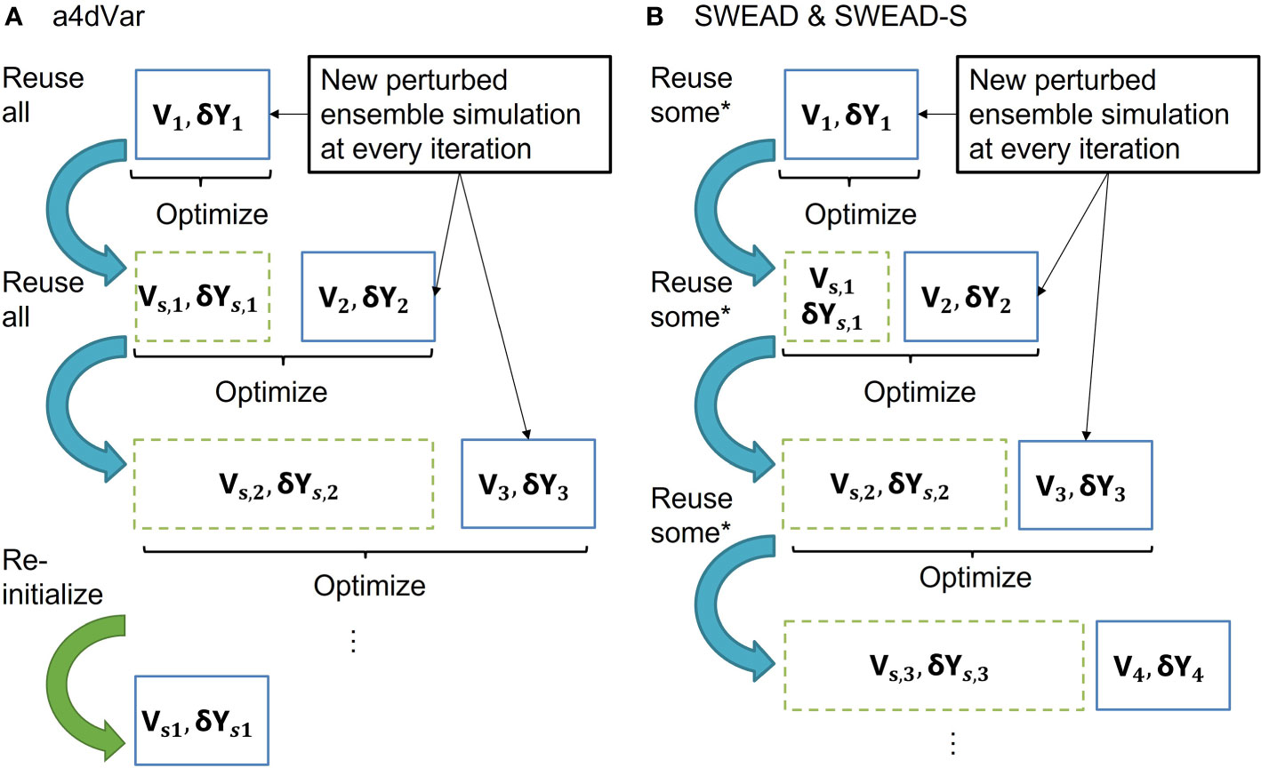
Figure 1 Schematic illustration of stacking algorithm for (A) a4dVar and (B) SWEAD and SWEAD-S. This figure is a modification of Fujimoto and Waseda (2020). © American Meteorological Society. Used with permission.

2.3 Proposed method: SWEAD-S

The following sections explain what is changed in SWEAD-S from SWEAD, taking deep-water waves as an example.

2.3.1 Predictable zone and singular value decomposition

A wave group conveys wave energy and information, and the wave group velocity determines how far the wave field can be predicted from observed data. Wu (2004) and Qi et al. (2018) analyzed the predictable zone of linear deep-water waves. The predictable zone, which is an area confined by the lowest and fastest wave group velocities, becomes narrower if the measurement period is shorter, or if the directional spread of the wave becomes broader (see Figures 2, 3 of Qi et al. (2018)).

The predictable zone is related to the singular vectors of the Jacobian A, and its SVD is A=UΣV^* , where U and V are unitary matrices containing the left and right singular vectors. ∑ is a rectangular diagonal matrix with non-negative real numbers on its diagonal. Let V_o be the right singular vector corresponding to the kernel space Ker(A) and ${\mathbf{\text{V}}}_o^{\perp }$ be the right singular vector corresponding to the orthogonal complement space (Ker(A))^⊥ . Let ${\mathbf{\text{Σ}}}_o^{\perp }$ be the diagonal matrix with the singular value corresponding to ${\mathbf{\text{V}}}_o^{\perp }$; A=UΣV^* can be rewritten as $\mathbf{\text{ A}}={\mathbf{\text{UΣ}}}_o^{\perp }{\mathbf{\text{V}}}_o^{\perp }$. The structure of the matrices is illustrated in Figure 2. We assumed that the observed data were sparse, and the physical dimension N_phys (column) was larger than the observational dimension N_obs (row).

FIGURE 2

Figure 2 SVD of the Jacobian matrix A = U∑V^*.

The solution to Ax = y is:

$\begin{array}{ll}\mathbf{\text{x}}={\mathbf{\text{V}}}_o^{\perp }{\mathbf{\text{Σ}}}_o^{\perp -1}{\mathbf{\text{U}}}^{*}\mathbf{\text{y}}+{\mathbf{\text{V}}}_o\mathbf{\chi }.& (10)\end{array}$

χ is an arbitrary vector, and V_oχ corresponds to an indefinite part of the solution. The term ${\mathbf{\text{V}}}_o^{\perp }{\mathbf{\text{Σ}}}_o^{\perp -1}{\mathbf{\text{U}}}^{*}\mathbf{\text{y}}$ corresponds to a definite part of the solution known as the minimum-norm solution. From the observed data y, only the first term of the above equation can be calculated; the second term is unknown owing to the arbitrary vector χ. Therefore, the subspace spanned by ${\mathbf{\text{V}}}_o^{\perp }$ corresponds to the predictable zone.

If the wave system is linear, then the Jacobian A is approximated by the linear dispersion relationship as A'. For example, the linear dispersion relationship of deep-water waves is ω² = gk, where ω denotes the angular frequency, g denotes the gravitational acceleration, and k denotes the wavenumber. If the observed data are from a water level gauge and $\widetilde{\mathbf{\text{x}}}$ is the Fourier coefficient of the initial surface elevation, then (R^(−1/2)A'D^(1/2))_qr = exp [i(ω_rt_q)], where q is the index of time and r is the index of the angular frequency and wavenumber. The approximated Jacobian is also decomposed as A'= UΣV^*. An example of the right singular vectors ${\mathbf{\text{V}}}_o^{\perp }$ and singular values ${\mathbf{\text{Σ}}}_o^{\perp }$ are shown in Figure 3. Here, we assumed that the length of the time series of the water level gauge was 25T_p and that the spatial domain was 32λ_p, where T_p denoted the peak wave period and λ_p denoted the peak wavelength. This setting is the same as that of the twin experiment of this study, as described later in Section 3.2. The spatial extents of the right singular vectors were limited to< 25λ_p, as shown in Figure 3D, and depended on their wavenumber components, as shown in Figure 3C.

FIGURE 3

Figure 3 Approximated Jacobian obtained from the linear dispersion relation. (A) The real part of the approximated Jacobian A’, (B) the singular values of the approximated Jacobian, (C) the absolute values of the right singular vectors of the approximated Jacobian in the wavenumber domain, and (D) the absolute values of the right singular vectors transformed to the spatial domain.

2.3.2 Generating ensembles in the predictable zone

SWEAD uses Fourier modes, which are global bases and could be redundant for the limited predictable zone. SWEAD-S utilizes SVD to find the most effective perturbations to decrease the cost function.

The gradient is estimated with the approximated Jacobian and its SVD A'=UΣV^* as:

$\begin{array}{ll}{\mathbf{\text{A'}}}^{*}(\mathit{\text{A}}({\mathbf{\text{x}}}_n)-\mathbf{\text{y}})={\mathbf{\text{VΣ}}}^{*}{\mathbf{\text{U}}}^{*}(\mathit{\text{A}}({\mathbf{\text{x}}}_n)-\mathbf{\text{y}}).& (11)\end{array}$

Let a vector d be defined such that Vd = A′^*(A(x_n)−y), and then:

$\begin{array}{ll}\mathbf{\text{d}}={\mathbf{\text{Σ}}}^{*}{\mathbf{\text{U}}}^{*}(\mathit{\text{A}}({\mathbf{\text{x}}}_n)-\mathbf{\text{y}}).& (12)\end{array}$

d reflects larger singular values of the approximated Jacobian A' and the misfit and indicates the singular vectors that are most sensitive to the misfit. Therefore, SWEAD-S generates perturbations from the right singular vectors V corresponding to leading components of d. SWEAD-S automatically neglects V_o, which corresponds to the zero-singular value, and the generated ensembles are limited to the predictable zone.

As mentioned in Section 2.2, the perturbations for the next iteration V_n should be orthogonal to the stacked perturbations V_s,_n-1. After projecting the approximated Jacobian A' onto an orthogonal complement ${\mathbf{\text{V}}}_{s,n-1}^{\perp }$ of the projection operator ${\mathbf{\text{V}}}_{s,n-1}^{\perp }{\mathbf{\text{V}}}_{s,n-1}^{\perp *}$, SWEAD-S calculates SVD as described below:

$\begin{array}{ll}{\mathbf{\text{A'V}}}_{s,n-1}^{\perp }{\mathbf{\text{V}}}_{s,n-1}^{\perp *}={\mathbf{\text{UΣV}}}^{*}, \mathbf{\text{d}}={\mathbf{\text{Σ}}}^{*}{\mathbf{\text{U}}}^{*}(\mathbf{\text{A}}({\mathbf{\text{x}}}_n)-\mathbf{\text{y}}).& (13)\end{array}$

${\mathbf{\text{V}}}_{s,n-1}^{\perp }$ is obtained by the Gram–Schmidt orthogonalization method. SWEAD-S selects new perturbations V_n from V corresponding to leading components of d.

2.3.3 Updating the approximated Jacobian

If the approximated Jacobian is fixed, the optimization becomes slower because the non-linearity is not reflected in the perturbation generation, as demonstrated in Section 4. SWEAD-S updates the approximated Jacobian sequentially as A'V_n←δY_n .

From Eq. (2), the amplitudes of the spectral peaks and the rest are all normalized. However, because the non-linear wave interaction is active in a wavenumber range near the spectral peak, the generated perturbations should concentrate on the spectral peak. Therefore, V_n and the approximated Jacobian A' are restored to the original scale:

$\begin{array}{ll}{\mathbf{\text{V}}}_{\mathbf{\text{D}}n}\text{ = }{\mathbf{\text{D}}}^{\mathrm{1/2}}{\mathbf{\text{V}}}_n,\widetilde{\mathbf{\text{A}}}\text{'}\text{ = }\mathbf{A}\text{'}{\mathbf{\text{D}}}^{-1/2}.& (14)\end{array}$

The approximated Jacobian is projected to the subspace spanned by ${{\mathbf{\text{V}}}^{*}}_{\mathbf{\text{D}}n}$ with the projection operator ${\mathbf{\text{P}}}_{\mathbf{\text{D}}}={\mathbf{\text{V}}}_{\mathbf{\text{D}}n}{({\mathbf{\text{V}}}_{\mathbf{\text{D}}n}^{*}{\mathbf{\text{V}}}_{\mathbf{\text{D}}n})}^{-1}{\mathbf{\text{V}}}_{\mathbf{\text{D}}n}^{*}$ and updated with $\mathbf{\text{A}}\text{'}{\mathbf{\text{V}}}_n=\widetilde{\mathbf{\text{A}}}\text{'}{\mathbf{V}}_{\text{D}n}\to \mathbf{\delta }{\mathbf{Y}}_n$ as:

$\begin{array}{ll}\begin{array}{l}\widetilde{\mathbf{\text{A}}}\text{'}=\widetilde{\mathbf{\text{A}}}\text{'}+\widetilde{\mathbf{\text{A}}}\text{'}({\mathbf{\text{P}}}_{\mathbf{\text{D}}}-{\mathbf{\text{P}}}_{\mathbf{\text{D}}})\\ =\widetilde{\mathbf{\text{A}}}\text{'}+\widetilde{\mathbf{\text{A}}}\text{'}({\mathbf{\text{V}}}_{\mathbf{\text{D}}n}-{\mathbf{\text{V}}}_{\mathbf{\text{D}}n})({\mathbf{\text{V}}}_{\mathbf{\text{D}}n}^{\ast }{\mathbf{\text{V}}}_{\mathbf{\text{D}}n}{)}^{\mathrm{-1}}{\mathbf{\text{VD}}}_n^{\ast }\\ \leftarrow \widetilde{\mathbf{\text{A}}}\text{'}+(\mathbf{\delta }{\mathbf{\text{Y}}}_n-\mathbf{\text{A}}\text{'}{\mathbf{\text{V}}}_n)({\mathbf{\text{V}}}_{\mathbf{\text{D}}n}^{\ast }{\mathbf{\text{V}}}_{\mathbf{\text{D}}n}{)}^{\mathrm{-1}}{\mathbf{\text{V}}}_{\mathbf{\text{D}}n}^{\ast }\end{array}.& (15)\end{array}$

The second term on the right side of Eq. (11) indicates the updated δY_n−A′V_n  of the linear approximation δY = AV by changing the control variable x_n projected to the subspace spanned by V_Dn. By multiplying D^1/2 by both sides of Eq. (15), we obtain the following equation of updated A':

$\begin{array}{ll}\mathbf{\text{A}}\leftarrow \mathbf{\text{A}}\text{'}+(\mathbf{\text{δ}}{\mathbf{\text{Y}}}_n- \mathbf{\text{A}}\text{'}{\mathbf{\text{V}}}_n){({\mathbf{\text{V}}}_n^{\ast }\mathbf{D}{\mathbf{\text{V}}}_n)}^{-1}{\mathbf{\text{V}}}_n^{\ast }\mathbf{\text{D}}.& (16)\end{array}$

2.3.4 Criteria for perturbations to be reused

The Hessian matrix H of the cost function L(w_n) is:

$\begin{array}{ll}\mathbf{\text{H}}=\mathbf{\delta }{\mathbf{\text{Y}}}^{*}\mathbf{\delta }\mathbf{\text{Y}}+\mathbf{\sum }_{t=1}^{N_T}(A_t({\mathbf{\text{x}}}_n)-y_t){\mathbf{\text{V}}}^{*}{\mathbf{\nabla }}^2{\mathbf{\text{A}}}_t\mathbf{\text{V,}}& (17)\end{array}$

where A_t and y_t denote elements of A and y, respectively, in the time index t. N_T is the total number of time steps. Let S denote the second term on the right side of the equation; then, H=δY^*δY+S. Ensemble 4Dvar methods such as a4dVar can be regarded as a type of Gauss–Newton method because the second term S is truncated as H=δY^*δY. If x_n is close to the optimal solution, A_t(x_n)−y_t is small, and this approximation is reasonable. Otherwise, S should be considered for the optimization.

The following condition, called the secant condition, should hold for the H=δY^*δY+S and the gradient  ∇L(x_n) :

$\begin{array}{ll}\mathbf{\text{H}}{\mathbf{\text{w}}}_n=(\mathbf{\text{δ}}{\mathbf{\text{Y}}}^{*}\mathbf{\delta }\mathbf{\text{Y}}+\mathbf{\text{S}}){\mathbf{\text{w}}}_n={\mathbf{\text{V}}}^{*}\mathbf{\nabla }L({\mathbf{\text{x}}}_{n+1})-{\mathbf{\text{V}}}^{*}\mathbf{\nabla }L({\mathbf{\text{x}}}_n).& (18)\end{array}$

The secant condition underlies the derivation of quasi-Newtonian methods such as the Broyden–Fletcher–Goldfarb–Shanno (BFGS) formula (Nocedal and Wright, 2006).

Let us introduce ${\mathbf{w}}_n^{\text{'}}$, which satisfies the following equation:

$\begin{array}{ll}\mathbf{\delta }{\mathbf{\text{Y}}}^{*}\mathbf{\delta }\mathbf{\text{Y}}{\mathbf{w}}_n^{\text{'}}\equiv {\mathbf{\text{V}}}^{*}\nabla L({\mathbf{\text{x}}}_{n+1})-{\mathbf{\text{V}}}^{*}\nabla L({\mathbf{\text{x}}}_n).& (19)\end{array}$

SWEAD-S considers S by comparing w_n and ${\mathbf{\text{w}}}_n^{\text{'}}$. If δY^*δY and S are both diagonal matrices, then:

$\begin{array}{ll}\begin{array}{l}{({\mathbf{\text{w}}}_n)}_i=\frac{1}{{(\mathbf{\delta }{\mathbf{\text{Y}}}^{*}\mathbf{\delta }\mathbf{\text{Y}})}_{ii}+{(\mathbf{\text{S}})}_{ii}}{({\mathbf{V}}^{*}\mathbf{\nabla }L({\mathbf{\text{x}}}_{n+1})-{\mathbf{\text{V}}}^{*}\mathbf{\nabla }L({\mathbf{\text{x}}}_n))}_i\\ {({\mathbf{\text{w}}}_n^{\text{'}})}_i=\frac{1}{{(\mathbf{\delta }{\mathbf{\text{Y}}}^{*}\mathbf{\delta }\mathbf{\text{Y}})}_{ii}}{({\mathbf{\text{V}}}^{*}\mathbf{\nabla }L({\mathbf{\text{x}}}_{n+1})-{\mathbf{\text{V}}}^{*}\mathbf{\nabla }L({\mathbf{x}}_n))}_i.\\ \therefore \frac{{({\mathbf{\text{w}}}_n)}_i}{{({\mathbf{\text{w}}}_n^{\text{'}})}_i}-1=\frac{{(\mathbf{\text{S}})}_{ii}}{{(\mathbf{\text{δ}}{\mathbf{\text{Y}}}^{*}\mathbf{\delta }\mathbf{\text{Y}})}_{ii}}.\end{array}& (20)\end{array}$

${({\mathbf{\text{w}}}_n)}_i/{({\mathit{\text{w}}}_n^{\text{'}})}_i-1$ indicates the ratio of S compared with δY^*δY in each ensemble dimension. For the assumption H=δY^*δY to be valid, S should be suppressed. Therefore, only perturbations satisfying the following criterion are reused in SWEAD-S:

$\begin{array}{ll}\left|\frac{{({\mathbf{\text{w}}}_n)}_i}{{({\mathbf{\text{w}}}_n^{\text{'}})}_i}-1\right|<e_{TOL},& (21)\end{array}$

where e_TOL denotes the error tolerance. In SWEAD, the following criterion equation is used:

$\begin{array}{ll}\frac{\left|{({\mathbf{\text{w}}}_n)}_i-{({\mathbf{\text{w}}}_n^{\text{'}})}_i\right|}{{\mathit{\text{σ}}}_{wn}}<e_{TOL}.& (22)\end{array}$

σ_wn denotes the standard deviation of w_n. Fujimoto and Waseda (2020) did not offer a rationale for the old criterion in Eq. (22), but now the new criterion in Eq. (21) has a rationale.

For δY^*δY and S to both be diagonal matrices, δY^*δY needs to be an eigenvalue decomposed as δY^*δY = MΛM^*, where Λ denotes the eigenvalue matrix. δY^*δY is a Hermitian matrix and M is a unitary matrix; then, MM^*=M^*M=I . Although S has $N_{ens}^2$ elements, w_n and ${\mathbf{\text{w}}}_n^{\text{'}}$ are vectors of N_ens elements, and only N_ens elements of S can be estimated. We assumed that M^*SM is a diagonal matrix and estimated the N_ens diagonal elements using a heuristic approach:

$\begin{array}{ll}\mathbf{\delta }{\mathbf{\text{Y}}}^{*}\mathbf{\delta }\mathbf{\text{Y}}+\mathbf{S}=\mathbf{\text{M}}\mathbf{\Lambda }{\mathbf{\text{M}}}^{*}+\mathbf{\text{S}}=\mathbf{\text{M}}(\mathbf{\Lambda }+{\mathbf{\text{M}}}^{*}\mathbf{\text{SM}}){\mathit{\text{M}}}^{*}& (23)\end{array}$

After these matrices are replaced as δY←δYM , V←VM, and S←M^*SM, Eq. (18) still holds. δY^*δY and S are already diagonalized, and Eq. (20) is valid.

Note that the difference in gradients was approximated by:

$\begin{array}{ll}{\mathbf{\text{V}}}^{*}\mathbf{\nabla }L({\mathbf{\text{x}}}_{n+1})-{\mathbf{\text{V}}}^{*}\mathbf{\nabla }L({\mathbf{\text{x}}}_n)={\mathbf{\text{V}}}^{*}{\mathbf{\text{A}}}^{*}(\mathit{\text{A}}({\mathbf{\text{x}}}_{n+1})-\mathbf{y})-{\mathbf{\text{V}}}^{*}{\mathbf{\text{A}}}^{*}(\mathit{\text{A}}({\mathbf{\text{x}}}_n)-\mathbf{\text{y}})\approx \mathbf{\text{δ}}{\mathbf{\text{Y}}}^{*}(\mathit{\text{A}}({\mathbf{\text{x}}}_{n+1})-\mathit{\text{A}}({\mathbf{\text{x}}}_n)).& (24)\end{array}$

2.3.5 Inclusion of the regularization term

Eqs. (9) and (19) are rewritten to include the regularization term:

$\begin{array}{ll}(\mathbf{\delta }{\mathbf{\text{Y}}}^{*}\mathbf{\delta }\mathbf{\text{Y}}+{\mathbf{\text{V}}}^{*}\mathbf{\text{V}}){\mathbf{\text{w}}}_n=-\mathbf{\delta }{\mathbf{\text{Y}}}^{*}(\mathit{A}({\mathbf{\text{x}}}_n)-\mathbf{\text{y}})-{\mathbf{\text{V}}}^{*}\mathbf{\text{x}}& (25)\end{array}$

$\begin{array}{ll}(\mathbf{\delta }{\mathbf{\text{Y}}}^{*}\mathbf{\delta }\mathbf{\text{Y}}+{\mathbf{\text{V}}}^{*}\mathbf{\text{V}}){\mathbf{\text{w}}}_{\mathbf{\text{n}}}^{\text{'}}\equiv \mathbf{\delta }{\mathbf{\text{Y}}}^{*}(\mathit{\text{A}}({\mathbf{\text{x}}}_{n+1})-\mathit{\text{A}}({\mathbf{\text{x}}}_n))+{\mathbf{\text{V}}}^{*}{\mathbf{\text{Vw}}}_n.& (26)\end{array}$

Additionally, for the eigenvalue decomposition of δY^*δY, the background error covariance matrix is also considered:

$\begin{array}{ll}\mathbf{\delta }{\mathbf{\text{Y}}}^{*}\mathbf{\delta }\mathbf{\text{Y}}+{\mathbf{\text{V}}}^{*}\mathbf{\text{V}}={\mathbf{\text{MΛM}}}^{*}& (27)\end{array}$

$\begin{array}{ll}\mathbf{\delta }\mathbf{\text{Y}}\leftarrow \mathbf{\delta }\mathbf{\text{YM}}, \mathbf{\text{V}}\leftarrow \mathbf{\text{VM}}.& (28)\end{array}$

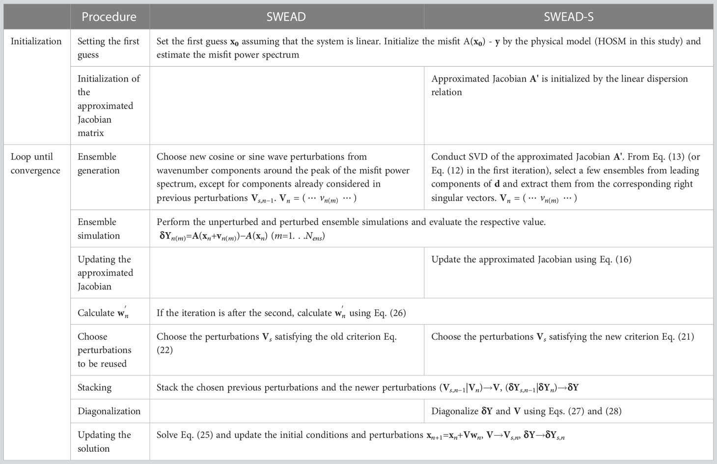
The differences between SWEAD and SWEAD-S are summarized in Table 1.

TABLE 1

Table 1 Scheme of SWEAD and SWEAD-S.

3 Twin experiment for non-linear deep-water waves

As described in Section 2.3.3, SWEAD-S updates the approximation of the Jacobian matrix, starting from the linear dispersion relationship. In this study, we tested SWEAD-S for deep-water waves, which are a typical example of non-linear dispersive waves.

Non-linearity is essential for accurately predicting propagation of deep-water waves (e.g., Mei et al., 2005). The third-order non-linearity increases the propagation speed of Stokes waves. If a is wave amplitude, then the angular frequency of the Stokes wave is ω²=gk(1+1/2 a²k²) . This equation means that the wave phase velocity ω/k increases with 1/2 a²k² . The third-order non-linearity could also increase the probability of large waves in irregular wave fields (Janssen, 2003). For irregular waves, H_m0 denotes the significant wave height, which is a typical wave height corresponding to 4σ, where σ is the standard deviation of the surface elevation. If the crest height of a wave is > 1.25H_m0, or if the wave height is > 2H_m0, the wave is commonly called a “freak wave” or “rogue wave” (Haver, 2004). Recent studies on non-linear deep-water waves have been summarized by Waseda (2019).

The higher-order spectral method (HOSM) (Dommermuth and Yue, 1987; West et al., 1987) is a promising method for predicting the propagation of non-linear deep-water waves and has been used in many studies (e.g., Ducrozet et al., 2007; Xiao et al., 2013; Bitner-Gregersen et al., 2020). The advantage of HOSM is that it can be applied to a wave field with a broad spectrum, like real ocean waves.

Some studies (Yoon et al., 2015; Wang and Pan, 2021) have applied the Kalman filter to HOSM. Additionally, other studies (Wu, 2004; Aragh et al., 2008; Blondel-Couprie et al., 2010; Blondel-Couprie et al., 2013; Qi et al., 2016; Köllisch et al., 2018) have applied the variational method to HOSM. The Kalman filter is adequate when the observed data are sufficient, but otherwise it might suffer filter divergence. We adopted the variational method in this study because it is relatively stable, even if the observed data are insufficient.

As described in the next section, HOSM is based on the Taylor expansion of governing equations of water waves and includes many expanded terms, which can make the implementation of the adjoint method for HOSM difficult. Therefore, SWEAD and SWEAD-S adopt the ensemble-based variational method.

3.1 Wave model: HOSM

Deep-water waves can be regarded as inviscid, irrotational, free-surface flows. The governing equations of deep-water waves are as follows (Zakharov, 1968):

The equation of continuity:

$\begin{array}{ll}\frac{{\partial }^2\varphi }{\partial z^2}=-{\nabla }^2\varphi , -d\le z\le \eta & (29)\end{array}$

The bottom boundary condition:

$\begin{array}{ll}\frac{\partial \Phi }{\partial z}=0 at z=-\infty & (30)\end{array}$

Kinematic free surface boundary condition:

$\begin{array}{ll}\frac{\partial \eta }{\partial t}+\nabla \Phi ·\nabla \eta =(1+{(\nabla \eta )}^2)Wat z=\eta & (31)\end{array}$

Dynamic free surface boundary condition (Bernoulli’s law):

$\begin{array}{ll}\frac{\partial \Phi }{\partial t}+\frac{1}{2}{(\nabla \Phi )}^2+g\eta =\frac{1}{2}(1+{(\nabla \eta )}^2)W^{2}at z=\eta ,& (32)\end{array}$

where

$$\begin{array}{l}\eta (x, y, t) \text{is the surface elevation}\\ \nabla =({\partial }_x, {\partial }_y): \text{is the nabla for the horizontal axis}\\ \Phi (x,y,t)=\varphi (x,y,z=\eta ,t) \text{is the velocity potential at the surface}\\ W={\partial }_z\varphi (x,y,z=\eta ,t) \text{is the vertical velocity at the surface}\\ g: \text{is the gravitational acceleration.}\end{array}$$

In the governing equations, the vertical surface velocity W is unknown. By assuming non-breaking waves, HOSM expands the vertical velocity as:

$\begin{array}{ll}W={\displaystyle \sum _{m=1}^M{w}^{(m)}}& (33)\end{array}$

$\begin{array}{ll}{w}^{(m)}={\displaystyle \sum _{l=0}^{m-1}\frac{{\eta }^l}{l!}\frac{{\partial }^{l+1}}{\partial z^{l+1}} {\varphi }^{(m-l)}{|}_{z=0}}& (34)\end{array}$

$\begin{array}{ll}\begin{array}{l}O(1):{\varphi }^{(1)}{|}_{z=0}=\Phi \\ O(m):{\varphi }^{(m)}{|}_{z=0}=-\sum _{l=1}^{m-1} \frac{{\eta }^l}{l!}\frac{{\partial }^l}{\partial z^l} {\varphi }^{(m-l)}{|}_{z=0},m\ge 2\end{array}& (35)\end{array}$

Substituting W with the free-surface boundary conditions in Eqs. (32) and (33) (West et al., 1987):

$\begin{array}{ll}\begin{array}{l}\frac{\partial \eta }{\partial t}=-\nabla \Phi ·\nabla \eta +{\displaystyle \sum _{m=1}^M{w}^{(m)}}+{(\nabla \eta )}^2{\displaystyle \sum _{m=1}^{M-2}{w}^{(m)}},\\ \frac{\partial \Phi }{\partial t}=-\frac{1}{2}{(\nabla \Phi )}^2-g\eta +\frac{1}{2}{\displaystyle \sum _{m=1}^{M-1}{w}^{(m)}{w}^{(M-m)}}\\ +\frac{1}{2}{(\nabla \eta )}^2{\displaystyle \sum _{m=1}^{M-3}{w}^{(m)}{w}^{(M-2-m)}}.\end{array}& (36)\end{array}$

HOSM solves these equations under periodic boundary conditions for utilizing the fast Fourier transform (FFT) to evaluate spatial derivatives. Because w^(m) consists of M terms of ϕ^(m)|_z=0  from Eq. (34), W involves O(M²) terms. HOSM can represent the free-surface boundary conditions accurately if terms of the fifth and higher orders are included, but this can result in boundary conditions that consist of several tens of terms.

3.2 Configuration of the twin experiments

To compare the performance of SWEAD and SWEAD-S, we conducted a twin experiment similar to that of Fujimoto and Waseda (2020). Time series of surface elevations were extracted from the output of the HOSM simulation initialized by a given spectrum and were contaminated by random noise. Those time series were considered as virtual observed data, which were assimilated into HOSM. Then, the whole wave field was estimated by SWEAD or SWEAD-S, and the true and estimated wave fields were compared.

HOSM generated a freak wave with a crest height of 1.5 H_m0. The generated wave field was taken as the truth. The power spectrum is a standard wave spectrum: the JONSWAP spectrum with γ = 3.3 (Hasselmann et al., 1973). The wave steepness was H_m0k_p/2=0.11 so that the non-linearity of the wave field was significant; k_p=2π/λ_p was the peak wavenumber. The computational domain for the initial simulation of the truth was 128λ_p to suppress the influence of the periodic boundary condition. In the wavenumber region, the computational domain spanned up to 8k_p (Tanaka and Yokoyama, 2004). According to Dommermuth (2000), a linear wave field gradually transitions to a non-linearly consistent wave field, including bound waves. The control variable x was set to the initial value of the water level before the non-linear spin-up (t=−5T_p). The time step was set to Δt=T_p/50 , and the fourth-order Runge–Kutta method was used.

The water level time series, including the freak wave, was used as the observed data (Figure 4). The white Gaussian noise was added to the time series, and the standard deviation was 10% of the standard deviation of the original water level time series. To emulate a situation in which the computational domain was redundant when compared with the predictable zone, the computational domain was set to 32λ_p (Figure 4), which was roughly twice as large as the linearly predictable zone corresponding peak wavenumber (LPZP) of 15λ_p for the observed time series 25T_p.

FIGURE 4

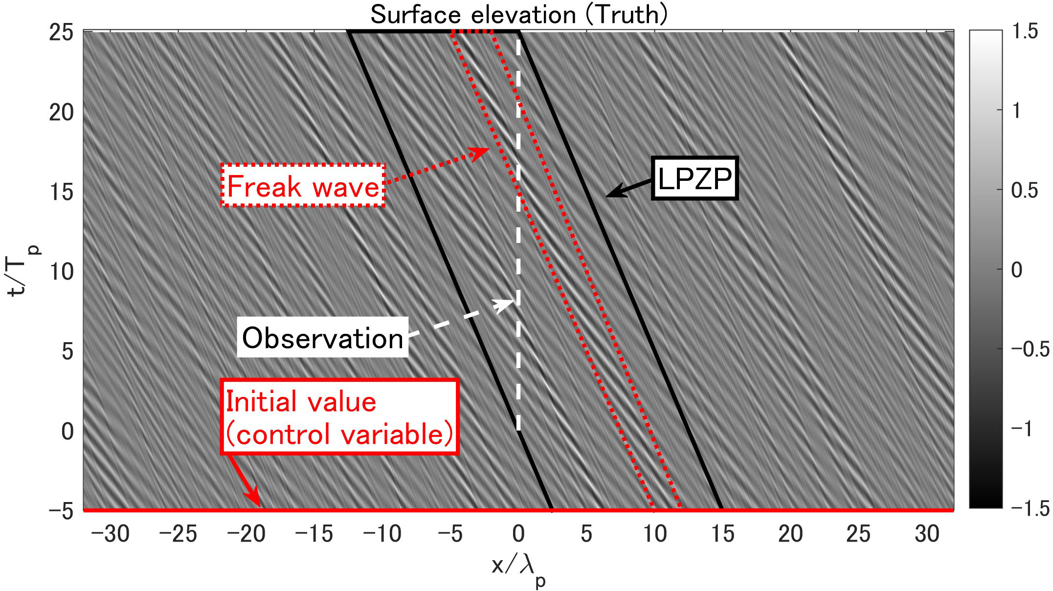
Figure 4 Generated truth (contours), measured points in the water level time series (dashed white lines), and linearly predictable zone corresponding peak wavelength (LPZP, solid black line). The wave groups, including the freak wave, are shown as red dotted lines. The initial value was taken as the control variable in the analysis.

Owing to insufficient observed data, the minimization of the cost function could be unstable. Regularization is a technique to stabilize a solution to an ill-posed problem by constraining the solution with prior information (Tikhonov and Arsenin, 1979). In SWEAD and SWEAD-S, the control variable $\widetilde{\mathbf{\text{x}}}$ is the Fourier coefficient of the initial wave field in the wavenumber space, and D is a diagonal matrix with a prior estimation of the power spectrum S(k) in its diagonal components, i.e., diag(D)= αS(k) . α is the regularization parameter. In this twin experiment, S(k) was the JONSWAP spectrum defined above. In reality, S(k) must be obtained by some other means, for example by spectral wave models such as WAVEWATCH III (Tolman, 2016). The regularization parameter α was determined to be α = 0.001 by the L-curve method (Hansen, 1992). Data assimilations were performed with 10 realizations of the noise with 10 ensembles N_ens=10 . e_TOL was selected as the best value for the old and new criteria: e_TOL = 0.2 and 0.5, respectively.

4 Results and discussion

The methods SWEAD and SWEAD-S were compared. As shown in Table 2, (a) is the conventional method, SWEAD, (b) is the SWEAD-S variant using the new criterion of reusing the perturbations in Eq. (21), and (c–e) are SWEAD-S variants, differing in whether they conduct the Jacobian update in Eqs. (12) and (13) and the diagonalization in Eq. (16).

TABLE 2

Table 2 Procedures of SWEAD and some variants of SWEAD-S.

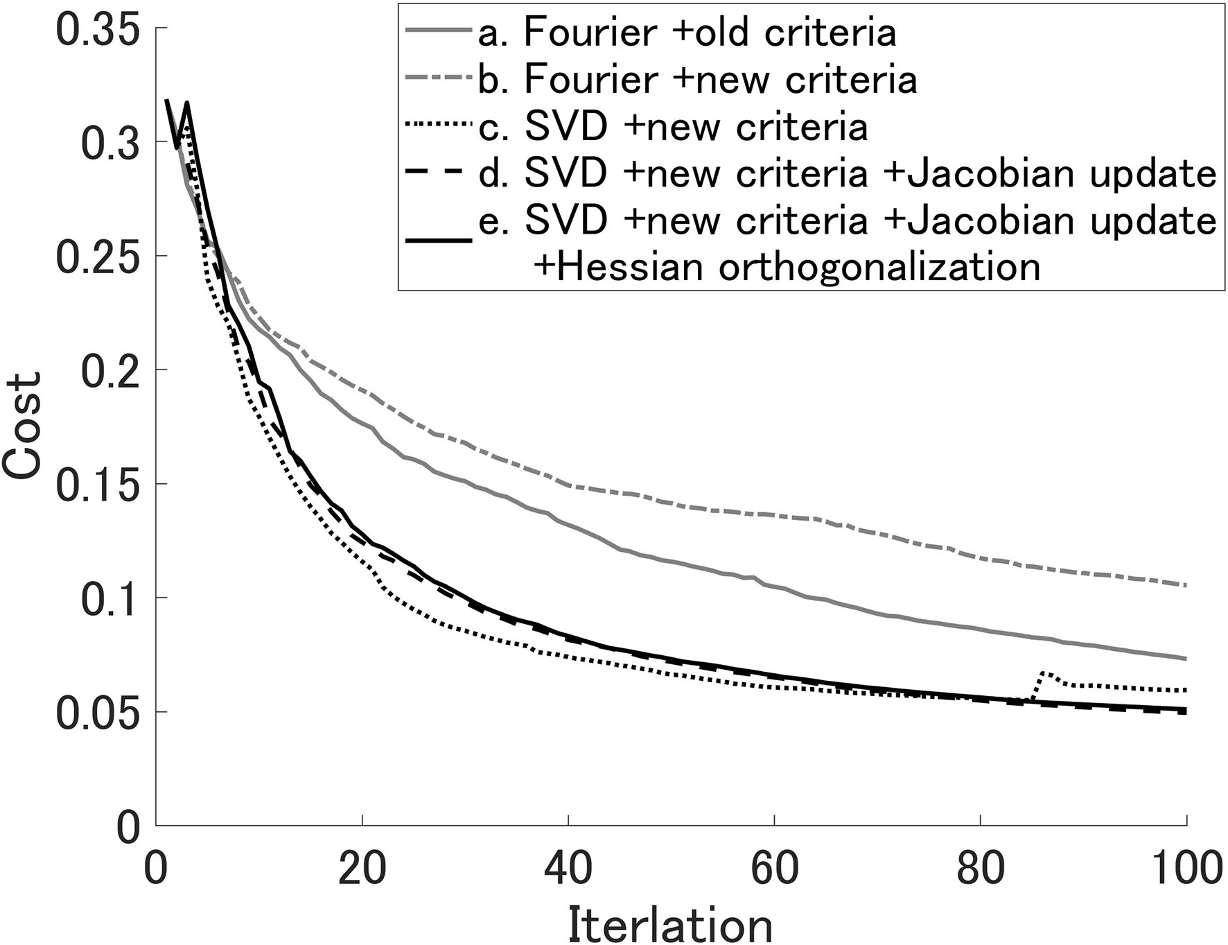
Figure 5 shows the root mean square error (RMSE) (Figure 5A) and correlation (Figure 5B) within the LPZP for each iteration averaged over the 10 realizations of the white Gaussian noise, and Figure 6 shows the averaged cost function for each iteration.

FIGURE 5

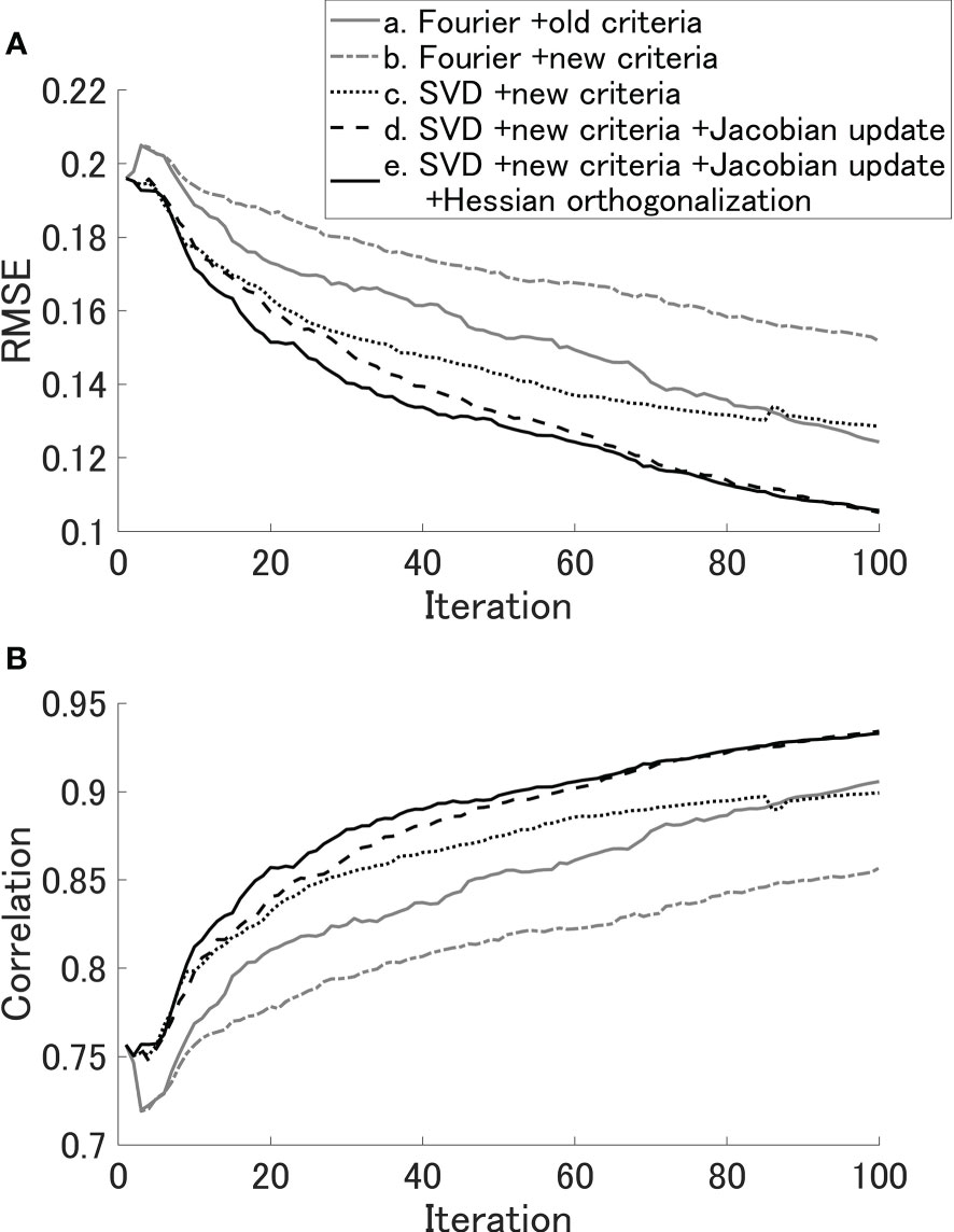
Figure 5 Estimation error within the LPZP averaged over the 10 realizations of the white Gaussian noise.

FIGURE 6

Figure 6 Cost function averaged over the 10 realizations of the white Gaussian noise.

4.1 Improvements by generating perturbations with SVD

SWEAD (a) and SWEAD-S (c) at the 20th iteration are compared in Figure 7. Because SWEAD (Figure 7A) did not explicitly consider the predictable zone in the ensemble generation, there was innovation, a difference between the analytical value and the linear first guess, beyond the LPZP. In contrast, as shown in Figure 7B, the innovation of SWEAD-S (c) was within the range of the LPZP because the SVD concentrated the search direction within the predictable zone.

FIGURE 7

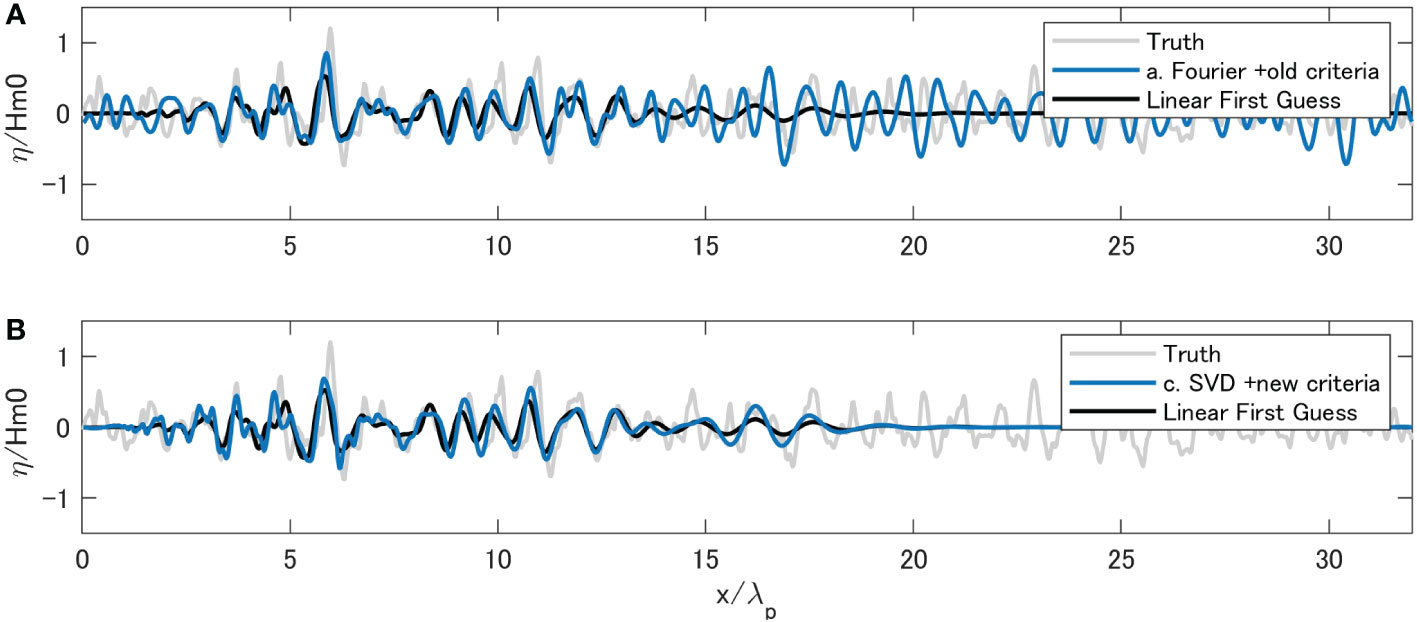
Figure 7 The analyses of SWEAD (a) and SWEAD-S variant (c) are compared to the truth and the linear first guess in panel (A, B), respectively.

The optimization efficiency of SWEAD-S (c) exceeded that of SWEAD (a) by up to approximately 85 iterations (Figure 5). However, SWEAD (a) caught up with the SWEAD-S variant that fixed the approximated Jacobian (c) in approximately 85 iterations (Figure 5). As described next, the method using SVD can be improved by updating the approximated Jacobian.

4.2 Improvements by updating the approximated Jacobian

The SWEAD-S variant with the updated Jacobian (d) optimized more efficiently than that without the updated Jacobian (c) after the 20th iteration (Figure 6). The variant with the updated Jacobian (d) also outperformed SWEAD (a) in terms of efficiency and accuracy (Figure 5). The correlation reached 0.9 in 94 iterations in SWEAD (a), but in 52 iterations in the SWEAD-S variant with the updated Jacobian (d). In other words, the SWEAD-S variant with the updated Jacobian (d) was twice as fast as SWEAD (a).

The reason for this improvement could be that the approximated Jacobian given by the linear dispersion relation (Figure 3) limited the predictable zone of each mode up to x = 25λ_p, which corresponds to the LPZP. Meanwhile, no such limit appeared in the updated approximated Jacobian (Figure 8). As shown in Figure 8B, the number of non-zero-singular values of the approximated Jacobian obtained after 100 iterations in the SWEAD-S variant with the updated Jacobian (d) was approximately 100. In contrast, that of the approximated Jacobian given by the linear dispersion relation was approximately 50 (Figure 3B). The spread of right singular vectors in the spatial dimension of SWEAD-S (e) increased from the linear dispersion relation, as shown in Figures 3D, 8D. Therefore, updating the approximated Jacobian is essential to expand the predictable zone. The non-linearity increases the wave group velocity, and the predictable zone should expand. It seems that this expansion of the predictable zone was reflected by the updates in the approximated Jacobian.

FIGURE 8

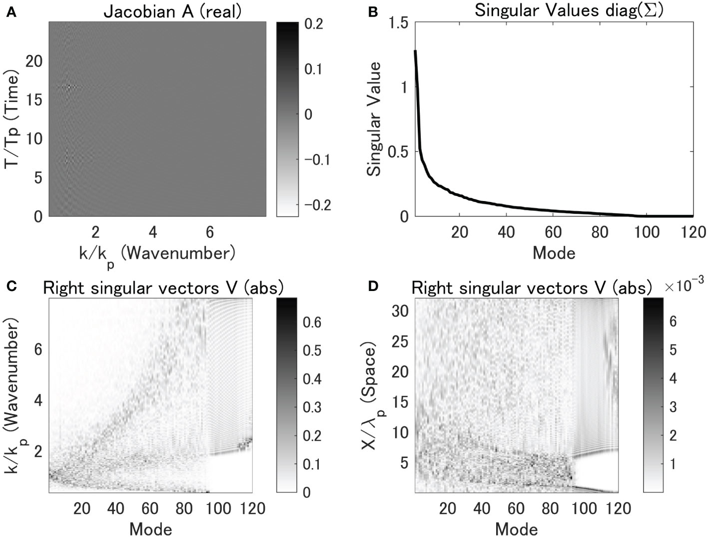
Figure 8 Approximated Jacobian obtained from the linear dispersion relation. (A) The real part of the approximated Jacobian A’, (B) the singular values of the approximated Jacobian, (C) the absolute values of the right singular vectors of the approximated Jacobian in the wavenumber domain, and (D) the absolute values of the right singular vectors transformed to the spatial domain.

4.3 Effects of different criteria on reusing perturbations

We confirmed that the old criterion in Eq. (22) resulted in an unstable optimization in SWEAD-S and then devised the new criterion in Eq. (21). Although the old criterion optimized faster than the new criterion in the SWEAD variant with the new criterion (b) (Figure 6), the SWEAD-S variants combining SVD and the new criterion formula (d, e) were the most computationally efficient among all cases.

The SWEAD-S variant with the diagonalization in Eqs. (27) and (28) (e) was optimized faster than the variant without diagonalization (d) at the early stage of the iteration, but variant (e) was caught up later by variant (d). Although the diagonalization was introduced to clarify the rationale of the new criterion equation, it had little advantage for optimization efficiency. As the optimization progresses, term S decreases, and the criterion equation should become uncritical.

The analytical values obtained after 100 iterations of the SWEAD-S method (e) are shown in Figure 9. As shown in Figure 4, the freak wave was located at approximately x = 10λ_p at t=−5T_p. In SWEAD-S, the freak wave was reproduced with sufficient accuracy.

FIGURE 9

Figure 9 Analytical values for the initial value (t = -5T_p) obtained after 100 iterations with SWEAD-S (e). The truth is shown as a black dashed line, and the analytical value is shown as a gray dashed line for each realization. The wave group leading to the freak wave existed around x/λ_p = 11 (Figure 4).

5 Conclusion

This study proposes the use of SWEAD-S, which uses the SVD of the approximated Jacobian to generate perturbations only in the predictable region. SWEAD-S updates the approximated Jacobian for generating ensembles, considering non-linearity. Furthermore, we devised a new criterion equation with a clear rationale for reusing perturbations by referring to the secant condition. This method is relevant where the physical system is weakly non-linear and a linear dispersion relation can roughly approximate the Jacobian. Non-linear deep-water waves are an appropriate example. We tested SWEAD-S using a twin experiment on a large wave called a freak wave, which was generated by HOSM. SWEAD-S reconstructed the freak wave well from only time series data of surface elevation. Furthermore, the optimization speed of SWEAD-S was twice as fast as that of SWEAD. Updating the approximated Jacobian contributes to improving the convergence speed and estimation accuracy by reflecting the expansion of the predictable zone due to non-linearity.

SWEAD-S is not limited to deep-water waves and might apply to other media of weakly non-linear dispersive waves. Nonetheless, strongly non-linear phenomena involving wave breaking are currently unsuitable for SWEAD-S. SWEAD-S is thought to apply to multi-directional waves; Fujimoto and Waseda (2020) demonstrated that SWEAD was applicable to a multi-directional wave field in a 32λ_p square, where the physical dimension of HOSM was O(~10⁵). However, a supercomputer was needed for such a high-dimensional problem, and a further decrease in computational burden is required. Storing the approximated Jacobian requires a large memory, limiting the dimensions of the physical space.

Data assimilation with a phase-resolved non-linear wave model such as HOSM will have many uses in both industry and academia. The wave field around ships or offshore structures could be monitored for marine safety. Additionally, the wave estimation itself could be a tool used for researching wave dynamics both in the ocean and in wave tanks. This study offers a theoretical framework for data assimilation of deep-water waves. However, SWEAD-S was assessed only via simulations; integrating the data assimilation technique and measurements remains challenging. Future studies could develop a method to represent modeling and observational errors in the ocean.

Data availability statement

The raw data supporting the conclusions of this article will be made available by the authors, without undue reservation.

Author contributions

WF: Investigation, conceptualization, methodology, software, writing-original draft. KI: Review and editing, project administration, resources. All authors contributed to the article and approved the submitted version.

Acknowledgments

The authors acknowledge Takuji Waseda, who provided valuable advice during preparation of the final version of the manuscript. We would like to thank Editage (www.editage.com) for English language editing.

Conflict of interest

WF and KI are employees of Nippon Kaiji Kyokai (ClassNK).

Publisher’s note

All claims expressed in this article are solely those of the authors and do not necessarily represent those of their affiliated organizations, or those of the publisher, the editors and the reviewers. Any product that may be evaluated in this article, or claim that may be made by its manufacturer, is not guaranteed or endorsed by the publisher.

References

Aragh S., Nwogu O., Lyzenga D. (2008). “Improved estimation of ocean wave fields from marine radars using data assimilation techniques,” in The Eighteenth International Offshore and Polar Engineering Conference (Vancouver, Canada) 8, 565. Available at: http://www.miseagrant.umich.edu/downloads/research/journals/08-330.pdf.

Google Scholar

Bitner-Gregersen E. M., Gramstad O., Magnusson A. K., Sames P. C. (2020). “Occurrence frequency of a triple rogue wave group in the ocean,” in Proceedings of the ASME 2020 39th International Conference on Ocean, Offshore and Arctic Engineering. Volume 2A: Structures, Safety, and Reliability (American Society of Mechanical Engineers: Virtual Conference, Online). doi: 10.1115/OMAE2020-19314

CrossRef Full Text | Google Scholar

Blondel-Couprie E., Bonnefoy F., Ferrant P. (2010). Deterministic non-linear wave prediction using probe data. Ocean Eng. 37, 913–926. doi: 10.1016/j.oceaneng.2010.03.002

CrossRef Full Text | Google Scholar

Blondel-Couprie E., Bonnefoy F., Ferrant P. (2013). Experimental validation of non-linear deterministic prediction schemes for long-crested waves. Ocean Eng. 58, 284–292. doi: 10.1016/j.oceaneng.2012.10.014

CrossRef Full Text | Google Scholar

Dommermuth D. G. (2000). The initialization of nonlinear waves using an adjustment scheme. Wave Motion 32, 307–317. doi: 10.1016/S0165-2125(00)00047-0

CrossRef Full Text | Google Scholar

Dommermuth D. G., Yue D. K. P. (1987). A high-order spectral method for the study of nonlinear gravity waves. J. Fluid Mech. 184, 267–288. doi: 10.1017/S002211208700288X

CrossRef Full Text | Google Scholar

Ducrozet G., Bonnefoy F., Le Touzé D., Ferrant P. (2007). 3-d HOS simulations of extreme waves in open seas. Natural Hazards Earth Syst. Sci. 7, 109–122. doi: 10.5194/nhess-7-109-2007

CrossRef Full Text | Google Scholar

Fujimoto W., Waseda T. (2020). Ensemble-based variational method for nonlinear inversion of surface gravity waves. J. Atmos. Ocean Technol. 37, 17–31. doi: 10.1175/JTECH-D-19-0072.1

CrossRef Full Text | Google Scholar

Hansen P. C. (1992). Analysis of discrete ill-posed problems by means of the l-curve. SIAM Rev. 34, 561–580. doi: 10.1137/1034115

CrossRef Full Text | Google Scholar

Hasselmann K., Barnett T. P., Bouws E., Carlson H., Cartwright D. E., Enke K., et al. (1973). Measurements of wind-wave growth and swell decay during the joint north Sea wave project (JONSWAP) (Deutches Hydrographisches Institut). Available at: http://repository.tudelft.nl/view/hydro/uuid%3Af204e188-13b9-49d8-a6dc-4fb7c20562fc/.

Google Scholar

Haver S. (2004). “A possible freak wave event measured at the draupner jacket January 1 1995,” in Rogue waves 2004 : proceedings of a workshop organized by Ifremer and held in Brest, France. 1–8. Available at: http://www.ifremer.fr/web-com/stw2004/rw/fullpapers/walk_on_haver.pdf.

Google Scholar

Janssen P. A. E. M. (2003). Nonlinear four-wave interactions and freak waves. J. Phys. Oceanogr. 33, 863–884. doi: 10.1175/1520-0485(2003)33<863:NFIAFW>2.0.CO;2

CrossRef Full Text | Google Scholar

Köllisch N., Behrendt J., Klein M., Hoffmann N. (2018). Nonlinear real time prediction of ocean surface waves. Ocean Eng. 157, 387–400. doi: 10.1016/j.oceaneng.2018.03.048

CrossRef Full Text | Google Scholar

Liu C., Xiao Q., Wang B. (2008). An ensemble-based four-dimensional variational data assimilation scheme. part I: Technical formulation and preliminary test. Mon. Weather Rev. 136, 3363–3373. doi: 10.1175/2008MWR2312.1

CrossRef Full Text | Google Scholar

Liu C., Xiao Q., Wang B. (2009). An ensemble-based four-dimensional variational data assimilation scheme. part II: Observing system simulation experiments with advanced research WRF (ARW). Mon. Weather Rev. 137, 1687–1704. doi: 10.1175/2008MWR2699.1

CrossRef Full Text | Google Scholar

Mei C. C., Stiassnie M., Yue D. K. P. (2005). Theory and applications of ocean surface waves (World Scientific).

Google Scholar

Nocedal J., Wright S. J. (2006). “Fundamentals of unconstrained optimization,” in Numerical optimization (New York, NY: Springer New York), 10–29. doi: 10.1007/978-0-387-40065-5_2

CrossRef Full Text | Google Scholar

Panteleev G., Yaremchuk M., Rogers W. E. (2015). Adjoint-free variational data assimilation into a regional wave model. J. Atmos. Ocean Technol. 32, 1386–1399. doi: 10.1175/JTECH-D-14-00174.1

CrossRef Full Text | Google Scholar

Qi Y., Wu G., Liu Y., Yue D. K. P. (2018). Predictable zone for phase-resolved reconstruction and forecast of irregular waves. Wave Motion 77, 195–213. doi: 10.1016/J.WAVEMOTI.2017.12.001

CrossRef Full Text | Google Scholar

Qi Y., Xiao W., Yue D. K. P. P. (2016). Phase-resolved wave field simulation calibration of sea surface reconstruction using noncoherent marine radar. J. Atmos. Ocean Technol. 33, 1135–1149. doi: 10.1175/JTECH-D-15-0130.1

CrossRef Full Text | Google Scholar

Saad Y., Schultz M. H. (1986). GMRES: A generalized minimal residual algorithm for solving nonsymmetric linear systems. SIAM J. Sci. Stat. Comput. 7, 856–869. doi: 10.1137/0907058

CrossRef Full Text | Google Scholar

Tanaka M., Yokoyama N. (2004). Effects of discretization of the spectrum in water-wave turbulence. Fluid Dyn. Res. 34, 199. doi: 10.1016/J.FLUIDDYN.2003.12.001

CrossRef Full Text | Google Scholar

Tikhonov A. N., Arsenin V. Y. (1979). Solutions of ill-posed problems. SIAM Rev. 21, 266–267. doi: 10.1137/1021044

CrossRef Full Text | Google Scholar

Tolman H. L. (2016). User manual and system documentation of WAVEWATCH III. (U. S. Department of CommerceNational Oceanic and Atmospheric Administration National Weather ServiceNational Centers for Environmental Prediction University Research Court College Park, MD 20740: Environmental Modeling CenterMarine Modeling and Analysis Branch).

Google Scholar

Wang G., Pan Y. (2021). Phase-resolved ocean wave forecast with ensemble-based data assimilation. J. Fluid Mech. 918, A19. doi: 10.1017/jfm.2021.340

CrossRef Full Text | Google Scholar

Waseda T. (2019). “Nonlinear processes,” in Ocean wave dynamics (Singapore: World Scientific), 103–161. doi: 10.1142/9789811208676_0004

CrossRef Full Text | Google Scholar

Waseda T., Watanabe S., Fujimoto W., Nose T., Kodaira T., Chabchoub A. (2021). Directional coherent wave group from an assimilated non-linear wavefield. Front. Phys. 9. doi: 10.3389/fphy.2021.622303

CrossRef Full Text | Google Scholar

Watanabe S., Fujimoto W., Nose T., Kodaira T., Davies G., Lechner D., et al. (2019). “Data assimilation of the stereo reconstructed wave fields to a nonlinear phase resolved wave model,” in Proceedings of the ASME 2019 38th international conference on ocean, offshore and Arctic engineering (Glasgow, Scotland, U.K: ASME). doi: 10.1115/OMAE2019-95949

CrossRef Full Text | Google Scholar

West B. J., Brueckner K. A., Janda R. S., Milder D. M., Milton R. L. (1987). A new numerical method for surface hydrodynamics. J. Geophys. Res. 92, 11803–11824. doi: 10.1029/JC092iC11p11803

CrossRef Full Text | Google Scholar

Wu G. (2004). Direct simulation and deterministic prediction of Large-scale nonlinear ocean wave-field (Boston: Massachusetts Institute of Technology), Vol. 258.

Google Scholar

Xiao W., Liu Y., Wu G., Yue D. K. P. (2013). Rogue wave occurrence and dynamics by direct simulations of nonlinear wave-field evolution. J. Fluid Mech. 720, 357–392. doi: 10.1017/jfm.2013.37

CrossRef Full Text | Google Scholar

Yaremchuk M., Martin P., Beattie C. (2017). A hybrid approach to generating search subspaces in dynamically constrained 4-dimensional data assimilation. Ocean Model. (Oxf) 117, 41–51. doi: 10.1016/j.ocemod.2017.08.003

CrossRef Full Text | Google Scholar

Yaremchuk M., Martin P., Koch A., Beattie C. (2016). Comparison of the adjoint and adjoint-free 4dVar assimilation of the hydrographic and velocity observations in the Adriatic Sea. Ocean Model. (Oxf) 97, 129–140. doi: 10.1016/j.ocemod.2015.10.010

CrossRef Full Text | Google Scholar

Yaremchuk M., Nechaev D., Panteleev G. (2009). A method of successive corrections of the control subspace in the reduced-order variational data assimilation*. Mon. Weather Rev. 137, 2966–2978. doi: 10.1175/2009MWR2592.1

CrossRef Full Text | Google Scholar

Yoon S., Kim J., Choi W. (2015). “An explicit data assimilation scheme for a nonlinear wave prediction model based on a pseudo-spectral method,” in IEEE Journal of Oceanic Engineering. 1. doi: 10.1109/JOE.2015.2406471

CrossRef Full Text | Google Scholar

Zakharov V. E. (1968). Stability of periodic waves of finite amplitude on the surface of a deep fluid. J. Appl. Mech. Tech. Phys. 9, 190–194. doi: 10.1007/BF00913182

CrossRef Full Text | Google Scholar

Zupanski M. (2005). Maximum likelihood ensemble filter: Theoretical aspects. Mon. Weather Rev. 133, 1710–1726. doi: 10.1175/MWR2946.1

CrossRef Full Text | Google Scholar