Laboratory study on movement characteristics of a river plume using particle image velocimetry

Rivers are important passages for land-based materials transported to the sea, such as fresh water, sediment, pollutants, and nutrients. River discharge with land-based materials will form a river plume with a buoyancy flow. The river plume is subject to the interaction between nearshore runoff with seawater. In this study, the movement characteristics of the river plume are investigated based on particle image velocimetry (PIV) and the dye tracing method. It is found that the change of flow rate and environmental water density will shape the river plume pattern in both the plan view and the side view. The combined effect of flow rate and environmental water density could be described by the Froude number. The river plume has a free surface in the x-z plane and the horizontal velocity of the plume can be fitted with a 1/2 Gaussian distribution curve. The change of flow rate has little effect on the type of plume thickness curve, while the increase of environmental water density will change the thickness curve type of the river plume. The stable thickness of the river plume increases with the increase of the Froude number. The maximum value of turbulent kinetic energy is located in the middle layer, and the increase of the flow rate or the density difference leads to the increase in the turbulent kinetic energy.

1 Introduction

Rivers are important passages for land-based materials transported to the sea. Lots of fresh water, sediment, pollutants, and nutrients are discharged into the adjacent sea area through estuaries. Land-based materials will directly affect the near-shore water environment and the aquatic ecological conditions. The impact area and the impact extent of land-based materials carried by rivers are primarily affected by the hydrodynamics of the river discharged into the sea. From the perspective of coastal environmental hydraulics, the discharge of rivers with land-based materials will form a river plume with a buoyancy flow. The river plume is the interaction between the nearshore runoff with the seawater (Cameron and Pritchard, 1963).

River plume has several characteristics that distinguishes it from pipe flow. The spatial scale of a river plume is much larger than that of a pipe flow. The river plume has a free surface and will move above the ambient water due to buoyancy. Similar to the jet or plume flow formed via a pipe, the movement and transport of river plume is driven by the momentum of the river and the dynamic conditions of the environmental water. Therefore, there are two main types of factors affecting the mixing and transport of river plume. One is the parameters related to the river plume itself, such as the flow rate, the estuary width, and the angle between river plume and coastline. The other is the parameters related to the environmental water, such as the water depth, the tidal current, and the wave. Due to the huge kinetic energy contained in the runoff, an interface of the upper freshwater layer and the lower salt water layer is formed. The interface shear is quite strong, resulting in the lower low-momentum and high-salinity water being swept and mixed by the upper flow (Garvine, 1975). At the same time, the various substances carried by the runoff, especially the pollutants and nutrients suspended in it, are also mixed and diluted by the mixing of freshwater with salt water.

Over the past decades, many researchers have conducted various studies on the river plume and analyzed the salinity change, the front structure, and dynamic process affected by it through field measurement data and the numerical simulation method. For example, Lentz (2004) developed a scale analysis theory to distinguish the features related to the river plume such as flow type, structure, and propagation velocity. Horner-Devine et al., (2009) provides a conceptual summary of the interaction between recirculated buoyancy flow and tides by cruise data. The tide modifies the structure of the plume in the region near the river mouth. The tidal plume flows over the top of the re-circulating plume and is typically bounded by strong fronts that may penetrate well below the re-circulating plume water and eventually spawn internal waves that mix the re-circulating plume further. In addition to the tide, the dynamic action of environmental fluid also includes wind and wave. The influence mechanism of wind on the mixing of estuarine plumes is different from that of tidal current. The wind increases the turbulence intensity on the surface of the flow, thereby enhancing the mixing effect of river plumes and ambient fluid. The wind also generates wind-driven flow on the surface of the water, affecting the movement track of river plumes (Nezlin and DiGiacomo, 2005; Feddersen et al., 2016; Rijnsburger et al., 2018; Qu and Hetland 2019). The impact of waves on river plumes is mainly that the frontal incoming waves increase the broadening of river plumes (Nardin et al., 2013).

However, the field observation of a river plume has certain limitations, which cannot accurately realize the motion observation of all water masses within a certain range. Therefore, laboratory experiments are required as a supplement to conduct more targeted research on the structure and movement characteristics of a river plume. Yuan et al. (2011, Yuan and Horner-Devine 2013) compared the river plume in the laboratory with and without lateral limits and found that lateral spreading dramatically modifies the plume structure. The spreading plume layer consists of approximately linear density and velocity profiles that extend to the surface, whereas the channelized plume profiles are uniform near the surface. Yuan et al. (2018) studied the influence of periodically changing flow on coastal buoyancy flow through the laboratory rotating platform. It was found that the bulge geometry oscillates between a circular plume structure that extends mainly in the offshore direction, and a compressed plume structure that extends mainly in the alongshore direction. The oscillations result in periodic variations in the width and depth of the bulge and the incidence angle formed where the bulge flow re-attaches with the coastal wall.

Despite meaningful results from previous research, laboratory investigations of river plume are still insufficient. The effect of the buoyancy and the flow rate on the movement characteristics of the river plume has been less studied. In fact, the difference in density between the upper and lower fluid layers has a great influence on the change of fluid turbulence intensity and velocity. The mixing process and movement characteristics of a river plume under the effect of different buoyancy and the plume flow rate are comprehensively studied using particle image velocimetry (PIV) technology. The main contents of this paper are organized as follows. In Section 2, the experimental setup and PIV measuring system are briefly described. The results, including the river plume qualitative description, the river plume quantitative flow field, Gaussian distribution of horizontal velocity, the river plume thickness, and the turbulent kinetic energy of the river plume, are presented in Section 3. Finally, conclusions are summarized in Section 4.

2 Methodology

2.1 Experimental setup

As shown in Figure 1, the experiment was conducted in a rectangular tank (1.5m long, 0.6m wide, and 0.5m deep). The rectangular tank was made with transparent acrylic plates with a good light transmission. The river plume was discharged from the right side of the rectangular tank, and the left side was designed with extra length as a buffer to reduce the backflow. The source of the river plume is a constant water tank located 3.0m above the rectangular tank, which is connected to a rectangular channel through a pipe. The center of the river mouth water surface was defined as the origin of the Cartesian coordinate. x positive direction is right, representing the onshore coordinates; z positive direction is upward, representing vertical coordinates; y is alongshore coordinate. The mouth of the rectangular channel is submerged in the environmental water. The width of the rectangular channel is 5 cm and the slope is 0.16.

FIGURE 1

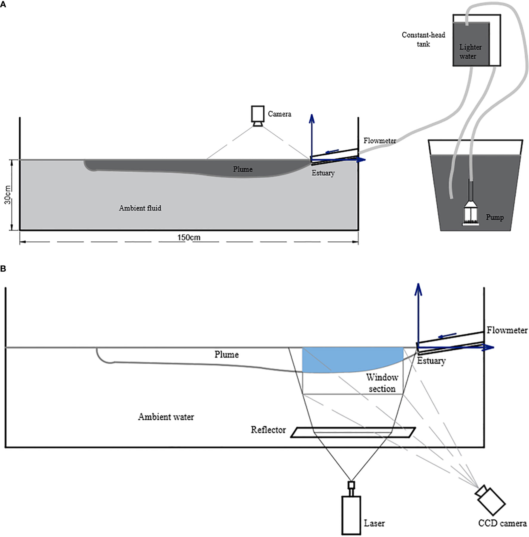
Figure 1 Diagram of the experimental setup: qualitative plan-view experiment (A) and qualitative and quantitative side-view experiment (B).

Two stages of experiment were designed in this study: the qualitative and the quantitative measurement. In the qualitative experiment, the plume was stained with dye, and two cameras were set above and in front of the rectangular tank, similar to the work of Pan et al. (2022). As a result, the planar view of the plume movement at the x-y plane and the side view at the x-z plane were captured. For quantitative experiments, the velocity of the plume movement at the x-z plane was recorded by the PIV system. The size of the field of view (FOV) was 35 cm × 12 cm.

2.2 PIV system and post-processing

The PIV system consists of a high-speed camera with 2-Gigabyte-memory storage and a continuous laser with a wavelength of 532nm. The resolution of the high-speed camera is 2048 × 2048 pixels. The camera framing rate was set to 200fps. The output power of the MGL-W-532 solid state laser was set to 8W. In the experiment, the incident light of the laser was parallel to the rectangular tank bottom and then was reflected by a plane mirror which had an angle of 45° with the bottom. As a result, the laser light could pass vertically upwards through the central axis of the river plume. The thickness of the laser light was about 2mm. Hence, the river plume was illuminated by the laser light. At the same time, tracer particles with a diameter of 50μm were added into the river plume.

A multi-grid interrogation method, which can increase the spatial and temporal resolution of flow field (Hsieh, 2008; Hsieh et al., 2016), was used in the post-processing stage. The multi-grid interrogation method consisted of three different interrogation window sizes: 32×32 pixels, 16×16 pixels, and 8×8 pixels. All passes adopted a 50% overlap between adjacent sub-windows. In traditional PIV image processing, a fixed time interval is usually used to calculate flow field. But if the velocity gradient is large (i.e., jet), adopting a fixed-time interval will inevitably result in bias error when calculating relatively small velocities. By adopting the multi-time interval method, the aforementioned bias error can be reduced. Four different time intervals (1, 3, 9, and 21) were used in this method; the most suitable time interval would be selected to reduce errors in the post-processing stage. Details of this multi-time interval algorithm can be found in Hsieh et al. (2016).

2.3 Experimental cases

In this study, nine cases of river plume were carried out for both the qualitative dyeing experiments and the velocity measurements. The specific parameters of the experimental cases are shown in Table 1. The effects of the buoyancy change and the flow rate on the movement characteristics of the river plume were examined.

TABLE 1

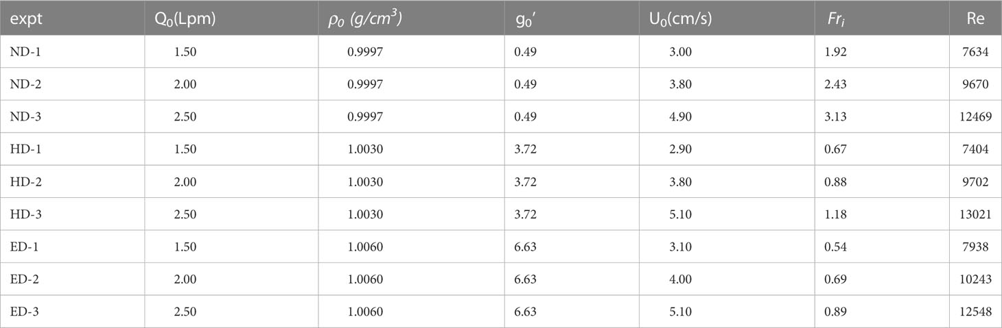
Table 1 The parameters of the experiments.

The initial velocity of the plume could be calculated by using the initial flow rate. The reduced gravitational acceleration was used to describe the effect of different buoyancies. Hence, the Froude number Fr_i, which is the ratio of inertial force to the buoyancy, could be described as

$\begin{array}{ll}{g}_0^{\prime }=\frac{{\rho }_0-\rho }{{\rho }_0}g& (1)\end{array}$

Where ρ₀ is the density of ambient fluid, ρ is the density of inflow, and g is gravitational acceleration,

$\begin{array}{ll}F{r}_i=\frac{U_0}{\sqrt{g_0^{\prime }{H}_0}}& (2)\end{array}$

Where U_0, $g_0^{\prime }$, and H₀ represent the velocity, reduced gravity, and the maximum depth of river plume inflow. The Reynolds number of each case is also listed in Table 1.

$\begin{array}{ll}\text{Re}=\frac{\rho U_0{H}_0}{\text{μ}}& (3)\end{array}$

Where μ represents the dynamic viscosity of the water.

In these cases, Fr_i ranges from 0.54 to 3.13. If Fr_i > 1, the flow is supercritical and if Fr_i < 1 the flow is subcritical. Re ranges from 7404 to 13021, indicating that the flow of each case is turbulent.

3 Result and discussion

3.1 Qualitative description of river plume

River plume generally enters the ocean from a channel with a certain gradient. In this study, the slope is set to 0.16. The dynamic processes of a river plume movement could be divided into the near-field process and the far-field process. In the near-field area, the initial velocity of the river plume causes the velocity shear and turbulence mixing with the sea water, and the density difference between the river plume and the sea water will cause a lateral expansion of the plume. In the far-field of the plume, the thickness of the plume tends to be stable and the mixing between the two water layers is weakened. The plan view and side view of the river plume in the qualitative experiments are illustrated in Figures 2, 3. All sets of the views were captured when the river plume was steady.

FIGURE 2

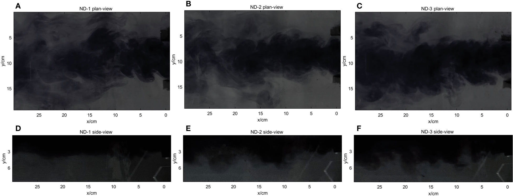
Figure 2 Plan and side view of plume with an ambient water density of 0.9997g/cm³: plan-view of Case ND-1,ND-2 and ND-3 (A–C),side-view of Case ND-1,ND-2 and ND-3 (D–F).

FIGURE 3

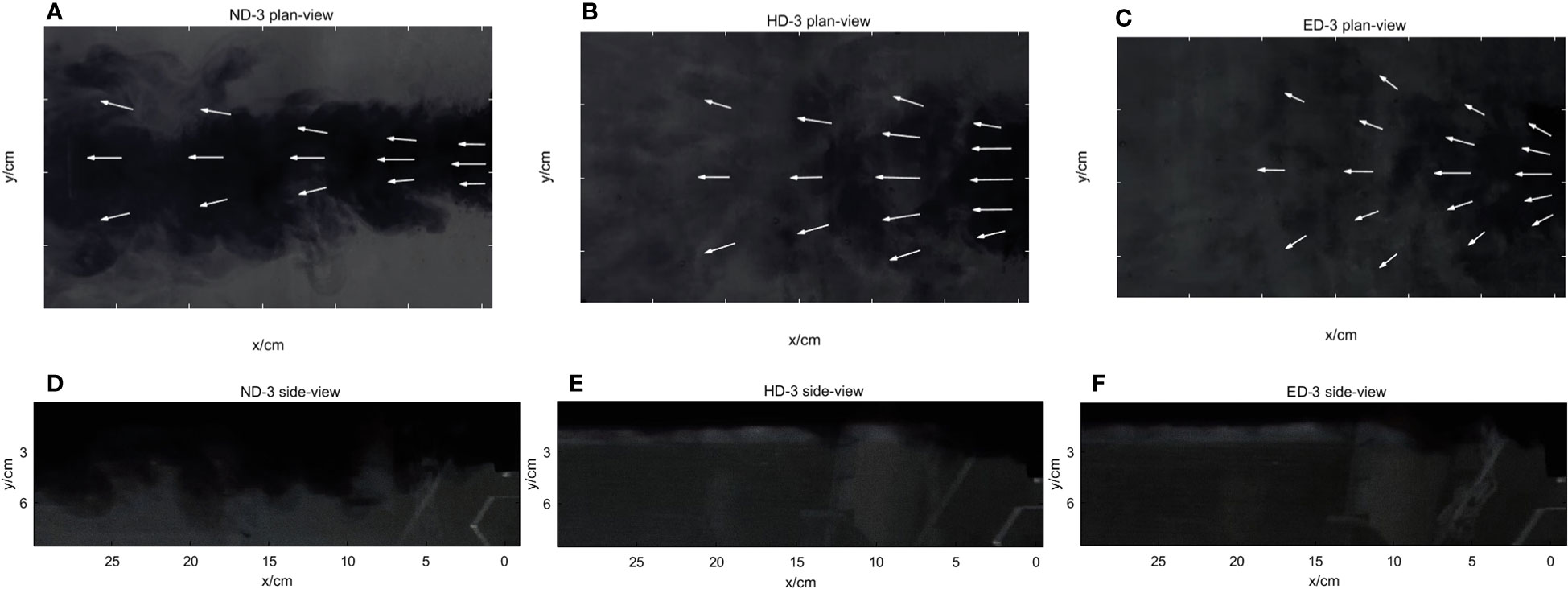
Figure 3 Plan and side view of plume with the flow rate of 2.5lpm: plan-view of Case ND-3, HD-3 and ED-3 (A–C),side-view of Case ND-3, HD-3 and ED-3 (D–F).

Figure 2 shows the qualitative description for cases ND-1, ND-2, and ND-3. The Froude number Fr_i of these three cases are larger than those in other cases; ND-3 is the largest of all groups and the flow is supercritical. For the plan view of these three cases, the river plume appears as jet-like currents with large offshore velocities and begins to show the tendency to expand laterally after maintaining the jet-like state. The change of plume shape caused by the increase of initial velocity shows that the lateral diffusion trend of plume decreases slightly within the observation range.

For the side view of these three cases, it is found that the plume maintains a steady state with a relatively constant thickness after a certain downward intrusion at the estuary. The stable thickness of the river plume in case ND-1 is obviously smaller than that in case ND-2 and case ND-3, and the stable thickness of the river plume in ND-3 is slightly greater than that in case ND-2. Comparing the pattern of mixing between the river plume and the ambient fluid, the mixing in case ND-1 is the weakest blending, and the interface between the river plume and the ambient fluid was the smoothest and most stable in the three cases. The mixing between the river plume and the ambient fluid in case ND-2 and case ND-3 at the interface was significantly stronger. The Kelvin–Helmholtz instability at the interface was more obvious in the two cases. In the observation of qualitative experiments, it is found that a more obvious vortex is formed when the front of the river plume interacts with the ambient fluid.

Figure 3 is the plan view and side view of the river plume at three ambient fluid densities at a flow rate of 2.5 LPM, namely case ND-3, case HD-3, and case ED-3. Among the three cases, ND-3 has the largest Fr_i, followed by Fr_i of HD-3, with Fr_i of ED-3 being the smallest.

In the sets of plan view, unlike case ND-3(high Fr_i) which shows a strong jet-like state, flows of case HD-3 and case ED-3 only maintain the offshore direction at the central axis and within a certain width, while the edge of the plume shows a clear lateral spread trend. In other words, the alongshore movement of the two plumes are significantly stronger than that in case ND-3. The higher the ambient fluid density is, the more obvious the lateral spread trend of the river plume is, and the river plume shape changes from a “trumpet” shape to “fan” shape.

In the sets of side views, the plume pattern of case HD-3 and case ED-3 are quite similar and differ greatly from case ND-3, and the Kelvin–Helmholtz instability at the interface gradually decreases with the increase of the ambient fluid density. That is to say, the increasing of the ambient fluid density limits the mixing at the interface between the river plume and the ambient fluid.

3.2 Flow field of river plume

The flow field of the river plume in all cases is shown in Figure 4. It is obvious that the flow field of the river plume is distributed with the maximum velocity at the surface layer. The velocity decreases gradually along the downward water depth, and the velocity of each layer of the river plume decreases gradually along the entrance toward the offshore direction. With the increase of the flow rate, the overall velocity of the river plume increases (the average surface velocities of HD-1, HD-2, and HD-3 are 2.2, 3.4, and 4.7 cm/s respectively); the high velocity range of plume also increases, while the low velocity range changes a little.

FIGURE 4

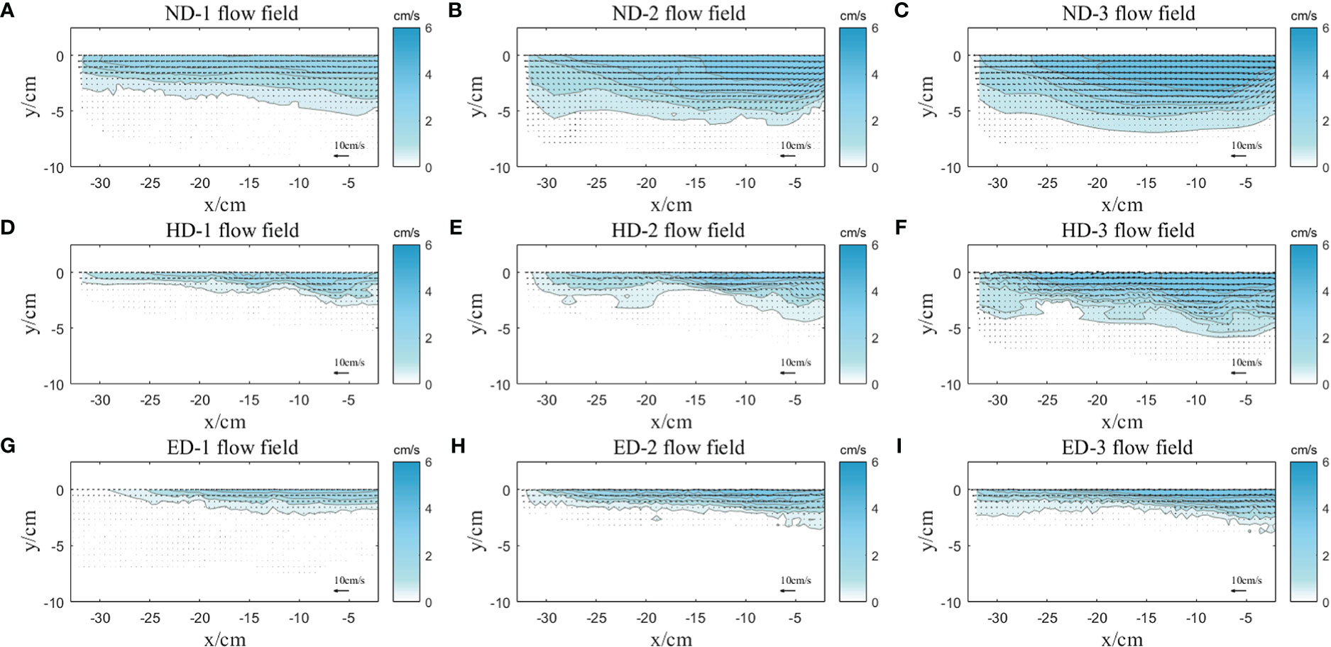
Figure 4 Flow field of the river plume in all cases: Case ND-1 (A), Case ND-2 (B), Case ND-3 (C),Case HD-1 (D), Case HD-2 (E), Case HD-3 (F), Case ED-1 (G), Case ED-2 (H) and Case ED-3 (I).

Due to the slope of the rectangular channel being 0.16, in case ND-2 and case ND-3, the direction of velocity vectors at the middle and bottom layer presents a downward direction deviating from the horizontal in the near mouth, but after moving for a distance under the buoyancy effect (relatively smaller than in HD and ED groups), they gradually change to deviating from the horizontal to the upward direction.

For the plume in case HD and ED groups, their velocity vectors all deviate from the horizontal upward direction near the river mouth. After moving to the surface, the velocity vector turns to the horizontal direction. It indicates that the buoyancy effect on the plume is obviously greater than the effect of its inertial force in these cases, and it is consistent with the phenomena in the plan view of Figure 3. Under the action of buoyancy, the flow in the lower layer gradually rises to the surface, and the fluid that was originally on the surface of the plume is pushed to two flanks.

3.3 Gaussian distribution of horizontal velocity

Zhao et al. (2019) fitted the vertical velocity of the vertically discharged buoyant flow with a Gaussian distribution curve and the vertical velocity in different water depths conforms to the curve well. The horizontal velocity distribution along the water depth of the river plume in this study also follows the Gaussian distribution well. The river plume has a free surface in the x-z plane, and the surface velocity is maximum. Therefore, this paper selects half of the Gaussian distribution to fit the horizontal velocity of the river plume and uses the axis of the Gaussian distribution to correspond to the horizontal velocity of the free surface, obtaining a good fitting effect. Yuan et al. (2018) used the variance of Gaussian distribution to define the width of plume in plan-view (b=Cσ). According to the experimental observation and freshwater conservation, C was set to 4, which was consistent with the width of buoyancy flow. In this study, we use C=2.2 to represent the horizontal velocity distribution width of each section because half of the Gaussian distribution was fitted with the data.

Figure 5 shows the fitting result of the horizontal velocity of each section for case ND-1, case ND-2, and case ND-3. The horizontal velocity of each section in the three cases increases significantly with the increase of flow rate and decreases with the increase of offshore distance. The distribution width of horizontal velocity also decreases along the river plume movement direction.

FIGURE 5

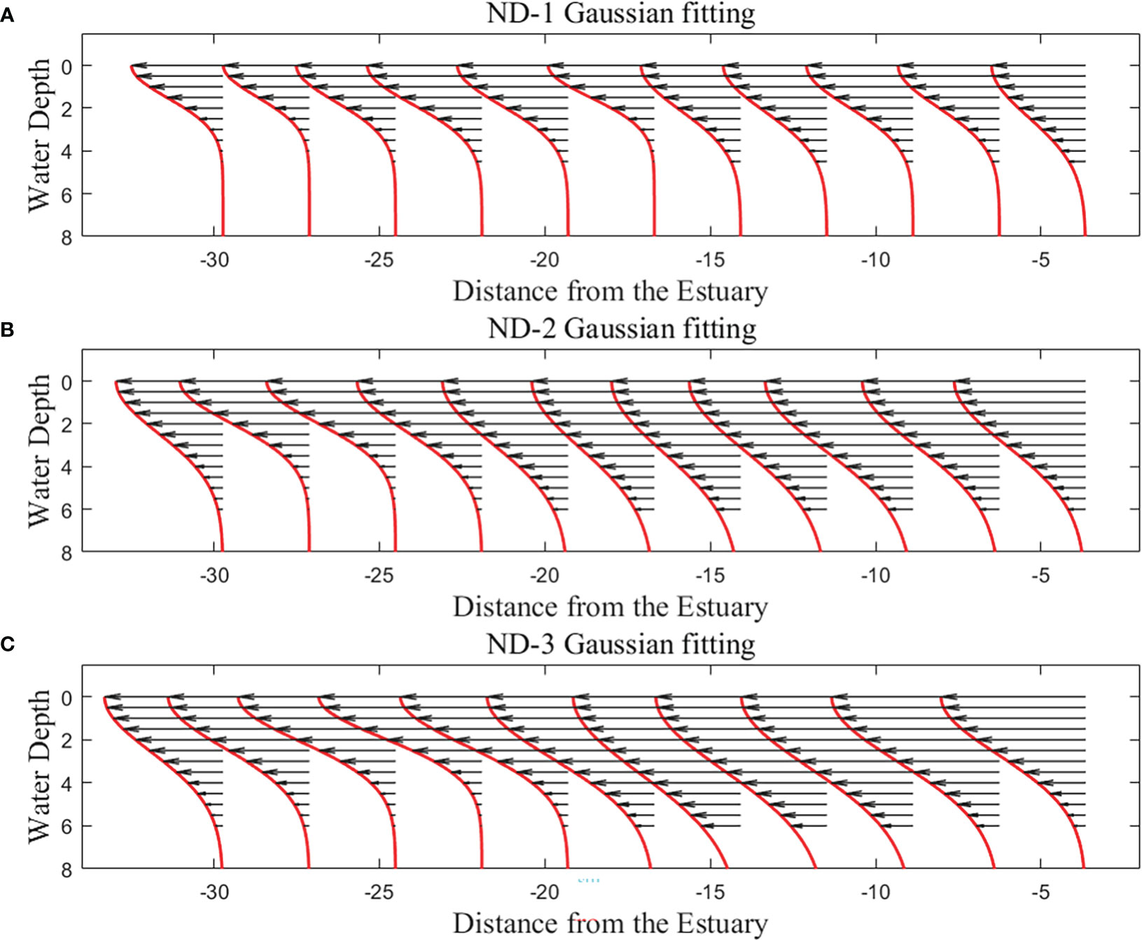
Figure 5 Gaussian distribution of horizontal velocity of ND groups: Case ND-1 (A), Case ND-2 (B) and Case ND-3 (C).

Figure 6 shows the fitting result of the horizontal velocity of each section for case ND-3, case HD-3, and case ED-3 under the condition that the plume flow rate is 2.5 LPM. The horizontal velocities of each section in the three groups change a little with the density of the environmental fluid, while the distribution width of the horizontal velocities change greatly. The increase of environmental fluid density reduces the width of horizontal velocity distribution at the same location, but each section still conforms well to the Gaussian distribution.

FIGURE 6

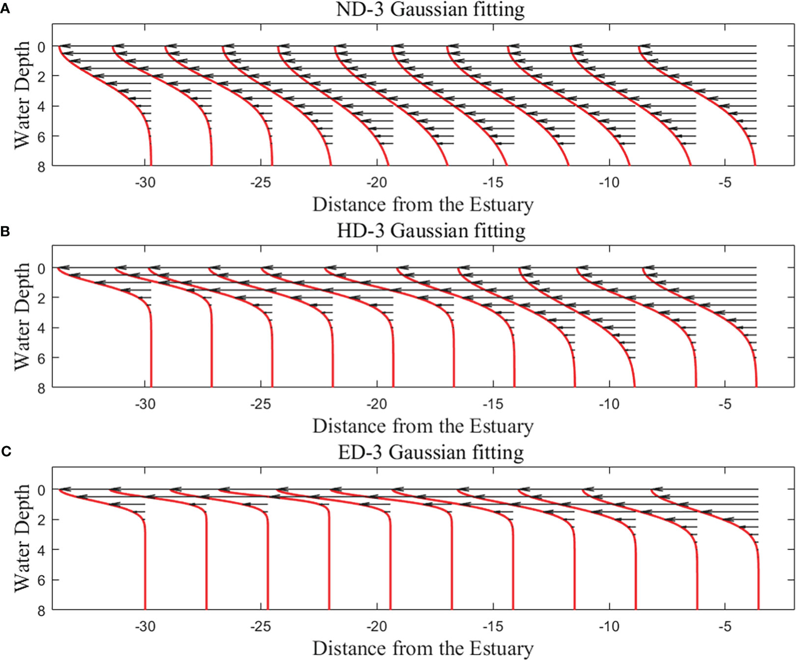
Figure 6 Gaussian distribution of horizontal velocity of D-3 groups: Case ND-3 (A), Case HD-3 (B) and Case ED-3 (C).

3.4 Thickness of the river plume

The water depth where the horizontal velocity drops to 1/e of the surface velocity is defined as the plume thickness in this study, which is similar to the definition of the half-width with a free jet. Starting from the maximum thickness location, the thickness scatter points of the river plume on each section were fitted with different types of curve, as shown in Figure 7.

FIGURE 7

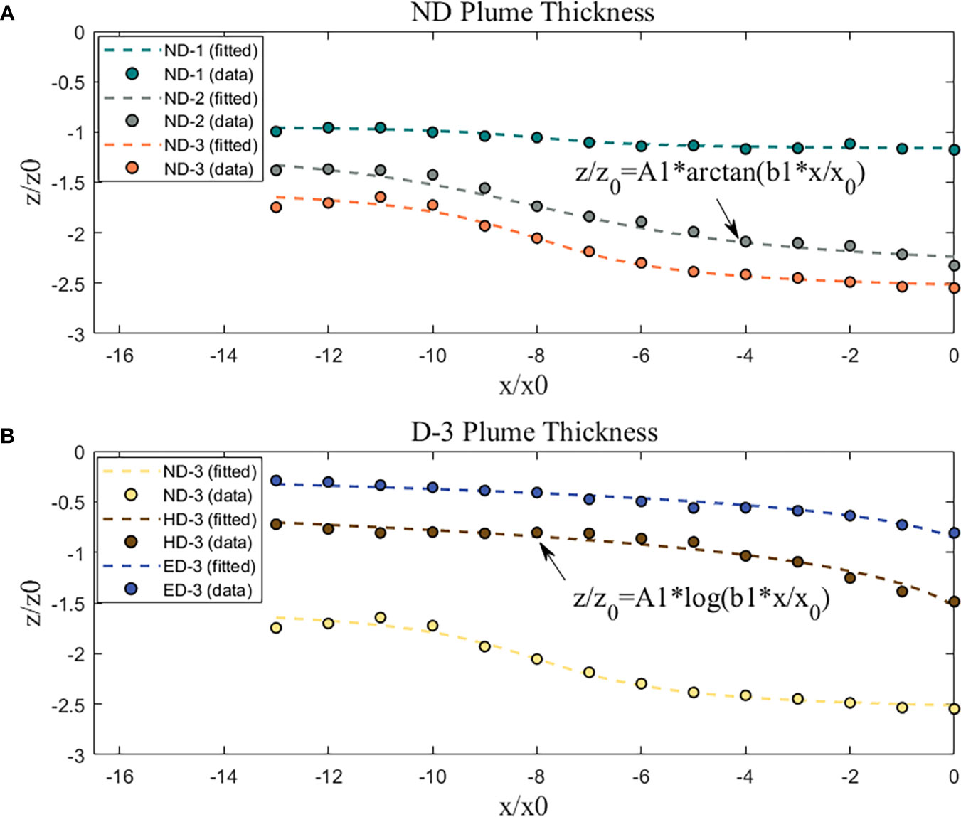
Figure 7 Thickness of river plume in different cases: ND group (A) and D3 group (B).

For the cases in the ND group, the densities of environmental water are the same. The thickness change along the river plume movement direction is similar in these cases, and the curve types do not change. All of them in these three cases are the inverse tangent function type, and the increase of flow rate only causes the change of parameter A1. The thickness in case ND-2 and case ND-3 increases first and then decreases along the river plume movement direction, and the decreasing of the flow rate makes the thickness curve tend to be flat. For the cases in the D-3 group, the change of the environmental water density causes a great change in the shape of the thickness curve. The shape of the thickness curve changes from an inverse tangent curve to a log curve with the increase of the environmental water density. The thickness curves of case HD-3 and case ED-3 are in the form of log curves. Compared with case HD-3, the environmental water density in case ED-3 is higher, resulting in the maximum thickness of plumes being smaller, the stable thickness being smaller, and the decreasing rate of the thickness from the maximum thickness to the stable thickness being significantly smaller.

Under the effects of the buoyancy and the inertial force, the upper and lower layer of water shear with each other and the plume thickness changes along the river plume direction. Figure 8 shows the relationship between the thickness of river plume after reaching stability with the Froude number Fr_i. The Froude number of case ED and HD groups is relatively small, and the stable thickness of the river plume will be small. The scattered points lie in the lower left corner. The Froude number of case ND group is relatively large, and as a result the stable thickness of river plume is also large. An obvious linear relationship could be found between the stable thickness of the river plume with the Froude number. It indicates that the Froude number is a key parameter to describe the behaviors of the river plume.

FIGURE 8

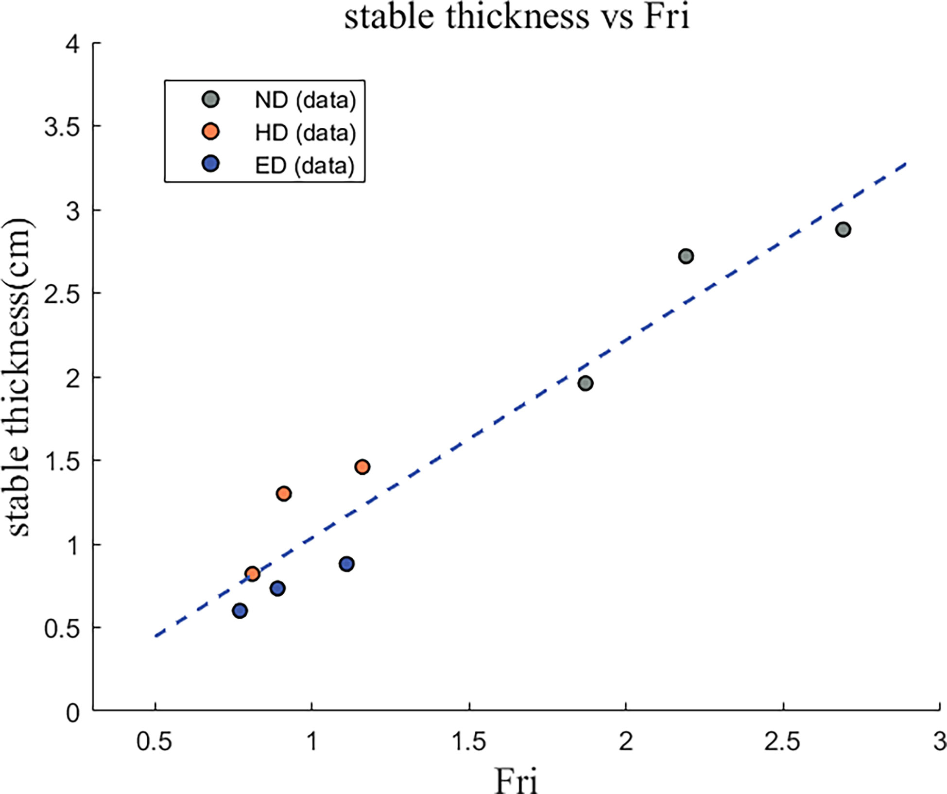
Figure 8 The relationship between the stable thickness and the Froude number.

3.5 Turbulent kinetic energy

Turbulent kinetic energy is an important parameter reflecting the turbulent characteristics of river plume. Turbulent kinetic energy is defined as follows:

$\begin{array}{ll}\text{k}=\frac{1}{2}(u_i^{\text{'}2}+v_i^{\text{'}2})& (4)\end{array}$

$\begin{array}{ll}{u}_i^{\text{'}}=u_i-{\overline{u}}_i& (5)\end{array}$

$\begin{array}{ll}{k}_{Ui}=\frac{1}{2}\frac{{\sum }_{i=1}^n{u}_i^{\text{'}2}}{n}=\frac{1}{2}\frac{{\sum }_{i=1}^n{(u_i-{\overline{u}}_i)}^2}{n}& (6)\end{array}$

$\begin{array}{ll}{k}_{Vi}=\frac{1}{2}\frac{{\sum }_{i=1}^n{v}_i^{\text{'}2}}{n}=\frac{1}{2}\frac{{\sum }_{i=1}^n{(v_i-{\overline{v}}_i)}^2}{n}& (7)\end{array}$

Where, k is turbulent kinetic energy and $u_i^{\prime }$ is the fluctuating velocity, defined as the D-value of velocity u_i and average speed ${\overline{u}}_i$. Therefore, the turbulent kinetic energy at the measuring point is k_{i =} k_Ui + k_Vi.

In the flow field, the turbulent kinetic energy k_i is used to represent the velocity fluctuating energy, that is, if the turbulent kinetic energy at a certain position is higher, there will be greater velocity fluctuating, and more energy transfer and dissipation.

We chose the section where the plume thickness is the largest as an example. The distribution of turbulent kinetic energy along the water depth in such a section was drawn in Figure 9. It is obvious that the increase of flow rate will cause the increase of turbulent kinetic energy. In each case, the maximum value of turbulent kinetic energy is located in the middle layer, and the turbulent kinetic energy gradually increases from the surface to the middle layer and then decreases to the bottom. The turbulent kinetic energy of the surface layer is obviously smaller than that of the middle layer. At the bottom boundary of the plume, the mixing of plume makes the velocity in this area reduce significantly. The increase of environmental water density will also enhance the turbulent kinetic energy. MacDonald and Geyer (2004) measured the velocities at three passes at the estuarine front in Fraser River, and the distribution shape of TKE production is quite similar to this study. TKE of the pass with higher salinity is significantly larger, and the peak is also closer to the upper layer. The results here verify the distribution pattern of TKE, and show the change of TKE under the influence of environmental water density and flow rate. A higher TKE production implies that the mixing between the river plume and the ocean will be increased and will enhance the exchange of substances.

FIGURE 9

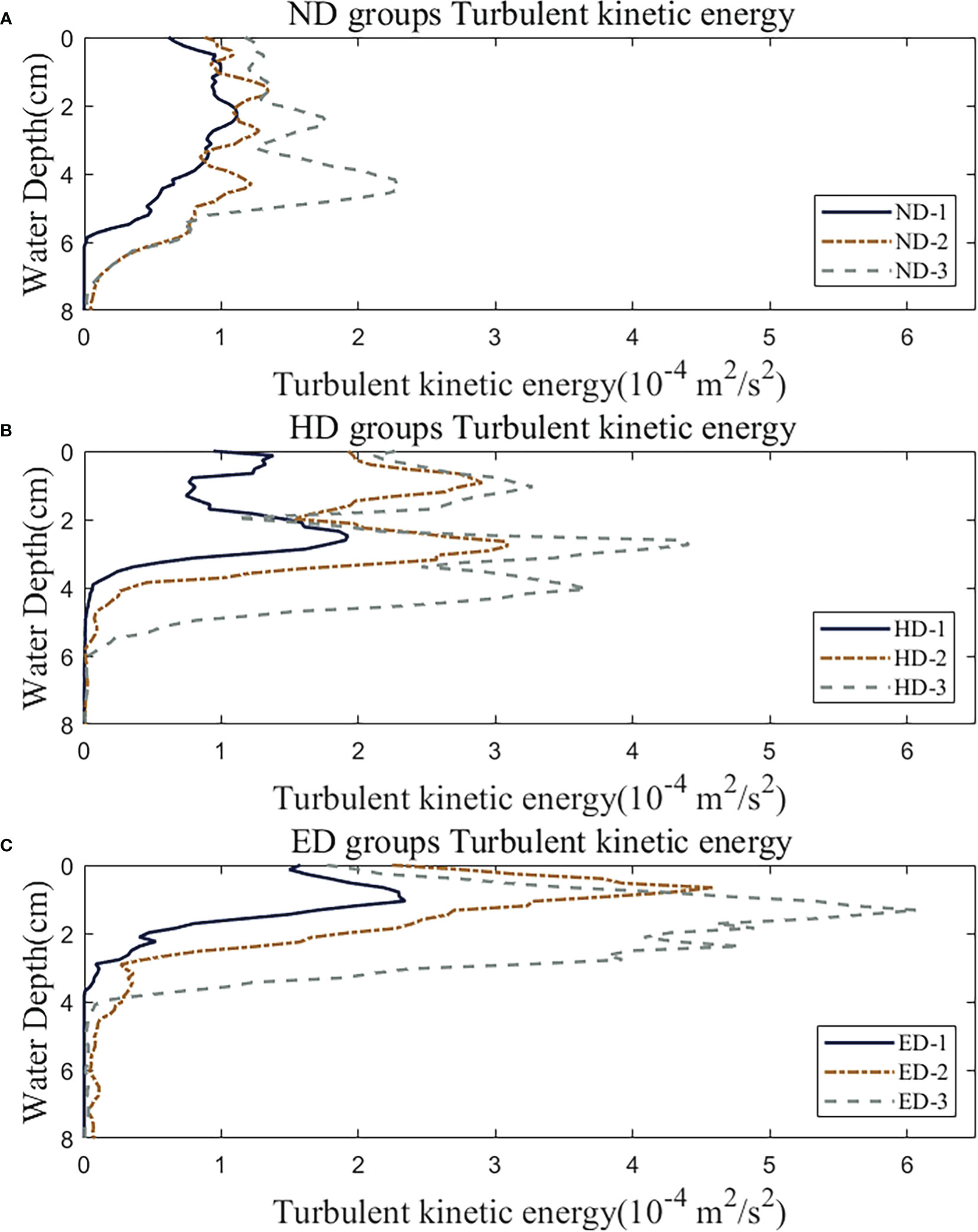
Figure 9 Turbulent kinetic energy at the maximum thickness section: ND group (A), HD group (B) and ED group (C).

4 Conclusions

In this study, the mixing process and movement characteristics of a river plume under the effect of different buoyancies and the plume flow rates are comprehensively studied using particle image velocimetry (PIV) technology. The main conclusions are summarized as follows.

(1) The change of flow rate and environmental water density will shape the river plume pattern in both the plan view and the side view. The combined effect of flow rate and environmental water density could be described by the Froude number.

(2) The river plume has a free surface in the x-z plane and the horizontal velocity of the plume could be fitted with a 1/2 Gaussian distribution curve.

(3) The thickness of the river plume increases with the increase of flow rate, and the increase in the density of ambient water changes the shape of the plume thickness curve from an arctan-type to log-type. The stable thickness of the river plume increases with the increase of the Froude number.

(4) The maximum value of turbulent kinetic energy is located in the middle layer, and the increase of the flow rate or the density difference leads to the increase in the turbulent kinetic energy.

Data availability statement

The original contributions presented in the study are included in the article/supplementary material. Further inquiries can be directed to the corresponding author.

Author contributions

ZX: conceptualization, methodology, formal analysis, and writing—review and editing. CX: experiment, and writing—original draft. GW: formal analysis and writing—review and editing. JZ: formal analysis, visualization, and writing—review. YC: writing—review and editing. All authors contributed to the article and approved the submitted version.

Funding

We are sincerely grateful for the support from the Key Research and Development Program of Hebei Province (21373302D), Marine Ecological Restoration and Smart Ocean Engineering Research Center of Hebei Province (HBMESO2308) and the National Natural Science Foundation of China (51979076).

Conflict of interest

The authors declare that the research was conducted in the absence of any commercial or financial relationships that could be construed as a potential conflict of interest.

Publisher’s note

All claims expressed in this article are solely those of the authors and do not necessarily represent those of their affiliated organizations, or those of the publisher, the editors and the reviewers. Any product that may be evaluated in this article, or claim that may be made by its manufacturer, is not guaranteed or endorsed by the publisher.

References

Cameron W. M., Pritchard D. W. (1963). “Estuaries,” in The Sea, vol. 2 . Ed. Hill M. N. (New York: Wiley), 306–324.

Google Scholar

Feddersen F., Olabarrieta M., Guza R. T., Winters D., Raubenheimer B., Elgar S. (2016). Observations and modeling of a tidal inlet dye tracer plume. J. Geophys. Res.: Oceans 121 (10), 7819–7844. doi: 10.1002/2016JC011922

CrossRef Full Text | Google Scholar

Garvine R. W. (1975). The distribution of salinity and temperature in the Connecticut river estuary. J. Geophys. Res. 80 (9), 1176–1183. doi: 10.1029/JC080i009p01176

CrossRef Full Text | Google Scholar

Horner-Devine A. R., Jay D. A., Orton P. M., Spahn E. Y. (2009). A conceptual model of the strongly tidal Columbia river plume. J. Mar. Syst. 78 (3), 460–475. doi: 10.1016/j.jmarsys.2008.11.025

CrossRef Full Text | Google Scholar

Hsieh S. C. (2008). Establishment of high time-resolved PIV system with application to the characteristics of a near wake flow behind a circular cylinder (Taiwan: National Chung Hsing University).

Google Scholar

Hsieh S. C., Low Y. M., Chiew Y. M. (2016). Flow characteristics around a circular cylinder subjected to vortex-induced vibration near a plane boundary. J. Fluids Structures 65, 257–277. doi: 10.1016/j.jfluidstructs.2016.06.007

CrossRef Full Text | Google Scholar

Lentz S. (2004). The response of buoyant coastal plumes to upwelling-favorable winds. J. Phys. oceanogr. 34 (11), 2458–2469. doi: 10.1175/JPO2647.1

CrossRef Full Text | Google Scholar

MacDonald D. G., Geyer W. R. (2004). Turbulent energy production and entrainment at a highly stratified estuarine front. J. Geophys. Res.: Oceans 109, C05004. doi: 10.1029/2003JC002094

CrossRef Full Text | Google Scholar

Nardin W., Mariotti G., Edmonds D. A., Guercio R., Fagherazzi S. (2013). Growth of river mouth bars in sheltered bays in the presence of frontal waves. J. Geophys. Res.: Earth Surface 118, 872–886. doi: 10.1002/jgrf.20057

CrossRef Full Text | Google Scholar

Nezlin N. P., DiGiacomo P. M. (2005). Satellite ocean color observations of stormwater runoff plumes along the San Pedro shelf (southern California) during 1997-2003. Continental Shelf Res. 25, 1692–1711. doi: 10.1016/j.csr.2005.05.001

CrossRef Full Text | Google Scholar

Pan Y., Yin S., Chen Y. P., Yang Y. B., Xu C. Y., Xu Z. S. (2022). An experimental study on the evolution of a submerged berm under the effects of regular waves in low-energy conditions. Coast. Eng. 176, 104169. doi: 10.1016/j.coastaleng.2022.104169

CrossRef Full Text | Google Scholar

Qu L., Hetland R. D. (2019). Temporal resolution of windforcing required for river plumesimulations. J. Geophys. Res.: Oceans 124, 1459–1473. doi: 10.1029/2018JC014593.

CrossRef Full Text | Google Scholar

Rijnsburger S., Flores R. P., Pietrzak J. D., Horner-Devine A. R., Souza A. J. (2018). The influence of tide and wind on the propagation of fronts in a shallow river plume. J. Geophys. Res.: Oceans 123, 5426–5442. doi: 10.1029/2017JC013422

CrossRef Full Text | Google Scholar

Yuan Y., Avener M. E., Horner-Devine A. R. (2011). A two-color optical method for determining layer thickness in two interacting buoyant plumes. Experiments fluids 50 (5), 1235–1245. doi: 10.1007/s00348-010-0969-y

CrossRef Full Text | Google Scholar

Yuan Y., Horner-Devine A. R. (2013). Laboratory investigation of the impact of lateral spreading on buoyancy flux in a river plume. J. Phys. Oceanogr. 43 (12), 2588–2610. doi: 10.1175/JPO-D-12-0117.1

CrossRef Full Text | Google Scholar

Yuan Y., Horner-Devine A. R., Avener M., Bevan S. (2018). The role of periodically varying discharge on river plume structure and transport. Continental Shelf Res. 158, 15–25. doi: 10.1016/j.csr.2018.02.009

CrossRef Full Text | Google Scholar

Zhao L., Zhang W., He Z., Tan L., Jiang H. (2019). The process of mass transport for a buoyant plume in linearly stratified environment. J. Shanghai Jiaotong Univ. 53 (04), 473–479. doi: 10.16183/j.cnki.jsjtu.2019.04.012

CrossRef Full Text | Google Scholar