Data driven three-dimensional temperature and salinity anomaly reconstruction of the northwest Pacific Ocean

By virtue of the rapid development of ocean observation technologies, tens of petabytes of data archives have been recorded, among which, the largest portion are those derived from the orbital satellites, embodying the character of ocean surface. Nevertheless, the insufficiency of information below the subsurface restricts the utilization of these data and the understanding of ocean dynamics. To circumvent these difficulties, we present the spatially three-dimensional reconstruction of ocean hydrographic profiles at depth based on the satellites and in-situ measurement data. In this manuscript, long short-term memory network (LSTM) and Gaussian process regression (GPR) methods are invoked to predict the temperature and salinity profiles in the northwest Pacific Ocean, and to improve computational and storage efficiency, the proper orthogonal decomposition (POD) method is subtly incorporated into these two models. LSTM and GPR show satisfactory results, with the root mean square error (RMSE) of temperature is less than 1.45, and the RMSE of salinity is less than 0.19. The incorporation of the POD method substantially accelerates efficiency, particularly in the LSTM model, which improves 7.5-fold without significant accuracy loss. The sensitivity of different sea surface parameters on the reconstructed profiles reveals that sea surface height anomaly and latitude significantly influence the reconstruction of temperature anomaly (TA) and salinity anomaly (SA) profiles. Besides, sea surface salinity and sea surface temperature anomalies can improve the model's estimation ability for the upper TAs and SAs, respectively. The contribution of monthly climatology to temperature and salinity profile estimation is also explored in this paper. It is shown that adding monthly mean climatology to the input of the model can achieve more accurate estimates.

1 Introduction

Ocean is an integral part of the global climate system and plays a crucial role in regulating climate change and balancing the Earth’s energy (Su et al., 2018). Knowledge of the vertical distribution of ocean temperature and salinity is significant for exploring the complex dynamical processes and ecosystems within the ocean (Rao and Sivakumar, 2003; Wilson and Coles, 2005; de Boyer Montégut et al., 2007; Helber et al., 2010; Meehl et al., 2011; Qin et al., 2015). However, the currently accumulated vertical temperature and salinity data is far from sufficient, and the problem of sparseness and discontinuity of the observed data due to the limitation of the number of observation points has severely limited the study of ocean processes and mechanisms (Klemas and Yan, 2014; Liu, 2016). Although the rapid development of satellite remote sensing technology has made it possible to provide more and more high-resolution, multi-scale and long-term continuous observation data, these data are limited to the ocean’s surface. They cannot provide spatial and temporal continuous information on the subsurface structure of the ocean (Ali et al., 2004; Wu et al., 2012; Bao et al., 2018). One fact is that the sea surface state is closely related to the subsurface features. According to the laws of ocean dynamics, many deep dynamic processes still generate signals at the sea surface, which satellite sensors can capture (Fiedler, 1988). Therefore, various underwater temperature and salinity reconstruction methods combining in situ observation data and satellite remote sensing data have been developed over the years.

One typical approach to reconstructing the internal structure from sea surface information is based on dynamics. Assimilation of observational data in numerical simulations (Ghil and Malanotte-Rizzoli, 1991; Troccoli and Haines, 1999; Vossepoel and Behringer, 2000; Carrassi et al., 2018; Moore et al., 2019) is a typical dynamics approach to inverse ocean subsurface information. However, this often requires many computing resources, and uncertainties in the initial and forced fields make the estimation accuracy impossible to guarantee (Robinson and Lermusiaux, 2000). Using a simplified dynamical framework can improve computational efficiency to some extent. Held et al. (Isern-Fontanet et al., 2006) proposes a method based on surface quasi-geostrophic (SQG) (Held et al., 1995) that derives subsurface density from sea surface density, sea surface height, and historical buoyancy frequency profiles. Further, Lapeyre and Klein (Lapeyre and Klein, 2006) developed an effective SQG (eSQG), assuming that the ocean interior’s potential vorticity (PV) is correlated with the surface density. eSQG was shown to be effective in improving subsurface flow field reconstructions (Isern-Fontanet et al., 2008; Qiu et al., 2016). Based on SQG, Wang et al. (Liu et al., 2017) proposed the internal + SQG (isQG) method, which superimposes the SQG mode with the positive and first oblique pressure modes to achieve subsurface density reconstruction by solving the surface quasi-geostrophic equation and the internal equation. The method’s effectiveness has been verified in different studies (Liu et al., 2014; Liu et al., 2017). However, due to the simplified model, some complex dynamical processes in the ocean are neglected (Liu et al., 2019; Meng and Yan, 2022), and the methods based on SQG can directly invert the density field, which will introduce additional errors when reconstructing the temperature and salinity fields (Chen et al., 2020).

Statistical methods are also widely used to reconstruct the three-dimensional structural field of the ocean. In earlier studies, linear regression (Willis et al., 2003; Nardelli and Santoleri, 2004; Guinehut et al., 2012) and least squares regression (Carnes et al., 1990; Carnes et al., 1994) were used to estimate deep ocean information. Besides, methods based on empirical orthogonal functions (EOF) (Maes et al., 2000; Meinen and Watts, 2000; Buongiorno Nardelli and Santoleri, 2005; Yan et al., 2020) are widely used to reconstruct the subsurface vertical structure. These methods use EOF to decompose the ocean vertical state vector, retain a few major modes, and then use least-squares regression or variational method (Fujii and Kamachi, 2003a; Fujii and Kamachi, 2003b) to solve for the objective function controlled by the sea surface information and the major modes. With the development of artificial intelligence techniques and machine learning methods, an increasing number of studies are focusing on the potential of machine learning methods in three-dimensional temperature and salinity field reconstruction. These methods can effectively mine the intrinsic patterns between data and estimate the structure of physical quantities in the ocean interior from sea surface parameters. Currently, self-organization mapping (Wu et al., 2012; Chen et al., 2018), support vector machine regression (Su et al., 2015; Li et al., 2017), random forest (Su et al., 2018), and neural network-based methods (Ali et al., 2004; Ballabrera-Poy et al., 2009; Bao et al., 2018; Lu et al., 2019; Buongiorno Nardelli, 2020; Su et al., 2020; Su et al., 2021) have been applied to estimate three-dimensional thermohaline fields. The results show that the machine learning methods can achieve better reconstruction based on a large amount of observation data and have strong generalizability.

In this context, this paper applies several different regression methods to estimate the subsurface temperature anomaly (TA) and subsurface salinity anomaly (SA). The first method used is Gaussian process regression (GPR) (Williams and Rasmussen, 1995; Rasmussen and Williams, 2005), an effective tool widely used in complex real-world problems (Stein, 1999; Forrester et al., 2008; Nguyen and Peraire, 2016). GPR is flexible enough to obtain estimates of unknown quantities using simple matrix operations and often achieves reliable accuracy on small data sets. More critically, it can effectively measure the uncertainty in the prediction because it gives the distribution of the predicted values (Rasmussen and Williams, 2005). The second one is the long short-term memory network (LSTM) (Hochreiter and Schmidhuber, 1997), a deep learning algorithm that can learn long-time dependencies (Sak et al., 2014; Wan et al., 2018; Yeo and Melnyk, 2019). However, training LSTM is often computationally expensive (Masuko, 2017), which is more fully reflected in ocean applications with ”big data” characteristics. Therefore, to reduce the training time and save storage costs, we further propose LSTM-POD and GPR-POD to predict the vertical distribution of TA and SA by introducing POD (Liang et al., 2002), a widely used tool for reduced order modeling (Lucia et al., 2004; Quarteroni et al., 2015). Specifically, POD can achieve simplification and dimensionality reduction of the dataset by identifying the few main modes that represent the three-dimensional temperature and salinity fields with relative precision. And then the TA and SA profiles can be approximated as linear combinations of these modes, we only need to learn the relationship between the coefficients and the input parameters by LSTM and GPR, which greatly simplifies the regression model. Therefore, the first goal of this paper is to explore the reconstruction accuracy of different models and the degree of improvement of the POD on computational efficiency. The reliability and computational efficiency of the proposed methods is verified by calculating the root mean square error (RMSE) between the estimated TA and SA profiles and the Argo thermohaline anomaly profiles, as well as comparing the CPU time of different methods. In addition, we point out that it is only necessary to interpolate the modes about the depth, and the linear combination of the interpolated modes according to the predicted coefficients can be used to obtain TA and SA estimates for any depth.

In particular, the effects of different parameters on TA and SA estimates are also investigated by comparing the prediction accuracy of models with various input parameters and calculating the correlation coefficients between input parameters and the temperature and salinity anomalies. In addition, this paper evaluates the potential application of climatology in temperature and salinity reconstruction using different combinations of temperature and salinity climatology data.

This paper is organized as follows. The study area and the data we used are presented in Section 2. Section 3 gives an overview of the methodology used in this paper. Section 4 is devoted to the description of the results, we draw conclusions in section 5.

2 Data

The goal of this paper is to reconstruct the three-dimensional thermohaline structure of the Northwest Pacific Ocean (95° W-135° W, 5° S-45° N) for the period 2011-2021. The sources of ocean observations used in this study are: Argo data, satellite sea surface temperature (SST), satellite sea surface salinity (SSS), and sea surface height anomaly (SSHA), which are described below. The climatology of the World Ocean Atlas 2018 (WOA18), used as the monthly mean of climatology is also presented.

2.1 Argo data

The Argo profiles are obtained from Global Sea Ocean Argo Scatter Dataset (V3.0) (Liu et al., 2021) provided by the China Argo Real-time Data Center (ftp://ftp.argo.org.cn/pub/ARGO/global/). This dataset collects more than 2.3 million temperature and salinity depth profiles observed by over 15,000 automated profiling buoys deployed in the global ocean by international Argo member countries during July 2000 through June 2020. Data inside the region of 95° W-135° W and 5° S-45° N for the period 2011-2021 are considered here. Profiles with depths exceeding 700 m are selected, and the profiles are interpolated through a spline into the same 71 vertical levels extending from the surface (5 m) to 705 m (vertical step is 10 m).

2.2 Satellite SST data

The SST data of this study are created by the OSTIA (Operational SST and Ice Analysis) system, using re-processed ESA SST CCI, C3S EUMETSAT and REMSS satellite data and in situ data from the HadIOD dataset, distributed through the Copernicus Marine Environment Monitoring Service (CMEMS, http://marine.copernicus.eu/services-portfolio/access-to-products/, product_id = SST_GLO_SST_L4_REP_OBSERVATIONS_010_011). This product provides daily maps of the SST and SST uncertainty on a global regular grid at 0.05° resolution, which are stored using the netCDF format using the Group for High Resolution SST specification.

2.3 Satellite SSS data

The SSS data is a Level 4 products on a 0.25 degree spatial and 4-day temporal grid produced by the International Pacific Research Center (IPRC) at the University of Hawaii at Manoa in collaboration with the Santa Rosa Remote Sensing System (RSS) in California in conjunction with observations from NASA’s Aquarius/SAC-D and Soil Moisture Active (SMAP) satellite missions. The product is a continuous, consistent multi-satellite SSS data obtained by optimal interpolation with a 7-day decorrelation time scale (Melnichenko et al., 2016). Their mean root mean squared difference from globally synchronized in situ data is about 0.19 psu and the product bias is about zero.

2.4 Satellite SSHA data

The altimeter sea level anomalies with daily and 0.25°×0.25° resolutions are provided by Sea Level TAC (Thematic Assembly Centre, https://resources.marine.copernicus.eu/product-detail/SEALEVEL_GLO_PHY_L4_MY_008_047/DATA-ACCESS). The data produced in the frame of this TAC are generated by the processing system including data from all altimeter Copernicus missions (Sentinel-6A, Sentinel-3A/B) and other collaborative or opportunity missions (e.g.: Jason-3, Saral[-DP]/AltiKa, Cryosat-2, OSTM/Jason-2, Jason-1, Topex/Poseidon, Envisat, GFO, ERS-1/2, Haiyang-2A/B/C).

2.5 Climatology data

The climate data used in this study are from World Ocean Atlas 2018 (Boyer et al., 2018) (https://www.ncei.noaa.gov/products/world-ocean-atlas), which is provided by the National Oceanographic Data Center (now the National Centers for Environmental Information - NCEI)(Boyer et al., 2018) (https://www.ncei.noaa.gov/products/world-ocean-atlas). The atlas is an objectively analyzed, quality-controlled collection of temperature, salinity, oxygen, phosphate, silicate, and nitrate averages based on profile data from the World Ocean Database and distributed online by NCEI. Monthly climatology fields of temperature and salinity at standard depth levels at a spatial resolution of 0.25°×0.25° were used in this study and interpolated by cubic spline onto regularly spaced vertical grids (10 m apart).

Note that all satellite data and climatology data are interpolated to the same spatial distribution as the Argo observations by bilinear interpolation in the present study. And anomalies are defined as the observation data (SST,SSS,Argo) subtracted by the monthly WOA18 data.

3 Method

3.1 Gaussian process regression

In this section, GPR is used to estimate the vertical profiles of TA and SA. The SAs and TAs in each level are considered as a collection of some random variables and obey a joint Gaussian distribution, defined as $y=f(x)+ϵ$, where $x$ is input vector of predicted parameters, which are sea surface temperature anomaly (SSTA), sea surface salinity anomaly (SSSA), sea surface height anomaly(SSHA), longitude (LON), latitude(LAT) and the day of the year projected on a circle (JULD). The prior distribution of $f(x)$ is assumed to be a GP given by $f(x)\sim GP(0,\kappa (x,x))$, and $\kappa$ is the semi-positive definite kernel. $ϵ\sim GP(0,{\chi }^2)$ denotes the Gaussian noise term, here $\chi$ is the standard deviation. Based on the historical Argo profiles and remote sensing data, we can collect $n$ TA observations or SA observations at depth $z$ to form the observation set $y=\left\{y_1,y_2,\dots ,y_n\right\}$. Corresponding to each observation, we have also collected a set of input parameters ${\mathbf{X}}_{\mathbf{\text{g}}}=[x_1\mid x_2\left|\dots \right|x_n]\in {ℝ}^{d\times n}$, here $x_i=(SST{A}_i,SSS{A}_i,SSH{A}_i,LO{N}_i,LA{T}_i,$ Then the prior distribution of $y$ can be given as:

$\begin{array}{ll}y|{\mathbf{X}}_{\mathbf{\text{g}}}\sim \mathcal{N}(0,{\mathbf{\text{K}}}_y),{\mathbf{\text{K}}}_y=\text{Cov}[y\mid {\mathbf{X}}_{\mathbf{\text{g}}}]=\kappa ({\mathbf{X}}_{\mathbf{\text{g}}},{\mathbf{X}}_{\mathbf{\text{g}}})+{\chi }^2{\mathbf{\text{I}}}_n.& (1)\end{array}$

GPR estimates the posterior distribution of an unknown quantity under the assumptions of a Gaussian process and the likelihood of a normal distribution. Specifically, from the above assumptions, it is known that the joint probability distribution of the estimated value $f_{*}$ at the new input parameter $x_{*}$ and the existing observation $y$ is a joint normal distribution of the following form:

$\begin{array}{ll}\left[\begin{array}{c}\mathit{y}\\ f_{*}\end{array}\right]\sim \mathcal{N}\left(0,\left[\begin{array}{cc}{\mathbf{\text{K}}}_y& {\mathbf{\text{K}}}_{*}\\ {\mathbf{\text{K}}}_{*}^{\text{T}}& {\mathbf{\text{K}}}_{**}\end{array}\right]\right),& (2)\end{array}$

where ${\mathbf{\text{K}}}_{*}=\kappa ({\mathbf{X}}_{\mathbf{\text{g}}},x_{*})$, ${\mathbf{\text{K}}}_{**}=\kappa (x_{*},x_{*})$. Combining the prior assumption and the likelihood, the posterior distribution of $f_{*}$ can be derived from the maximum likelihood method (Williams and Rasmussen, 1995),

$\begin{array}{ll}\begin{array}{l}{f}_{*}\mid x_{*},{\mathbf{X}}_{\mathbf{\text{g}}},y\sim GP(m^{*},C^{*}),\hfill \\ m^{*}={\mathbf{\text{K}}}_{*}^{\text{T}}{\mathbf{\text{K}}}_y^{-1}y,C^{*}={\mathbf{\text{K}}}_{**}-{\mathbf{\text{K}}}_{*}^{\text{T}}{\mathbf{\text{K}}}_y^{-1}{\mathbf{\text{K}}}_{*}.\hfill \end{array}& (3)\end{array}$

The reconstruction of TA and SA profiles using GPR is carried out in the python library (GPy, 2012), and the output is a vector consisting of the TA profile and SA profile in series at the same location. The kernel function chosen in this paper is the radial basis function. The minimum and maximum of the input/output can be utilized to scale the input/output to [0,1] to eliminate the magnitude effect before the model is trained.

In summary, the derivation of the vertical structure of TA and SA using GPR involves two processes: online and offline stages. In the offline stage, historical observations are collected to build the corresponding input/output training set, from which the GPR is trained to learn the mapping of the input parameters to the TA and SA profiles. In the online stage, the corresponding TA and SA profiles are estimated from the already trained GPR for the new input parameters. The flowchart of TA and SA estimation using the GPR is shown in Figure 1.

FIGURE 1

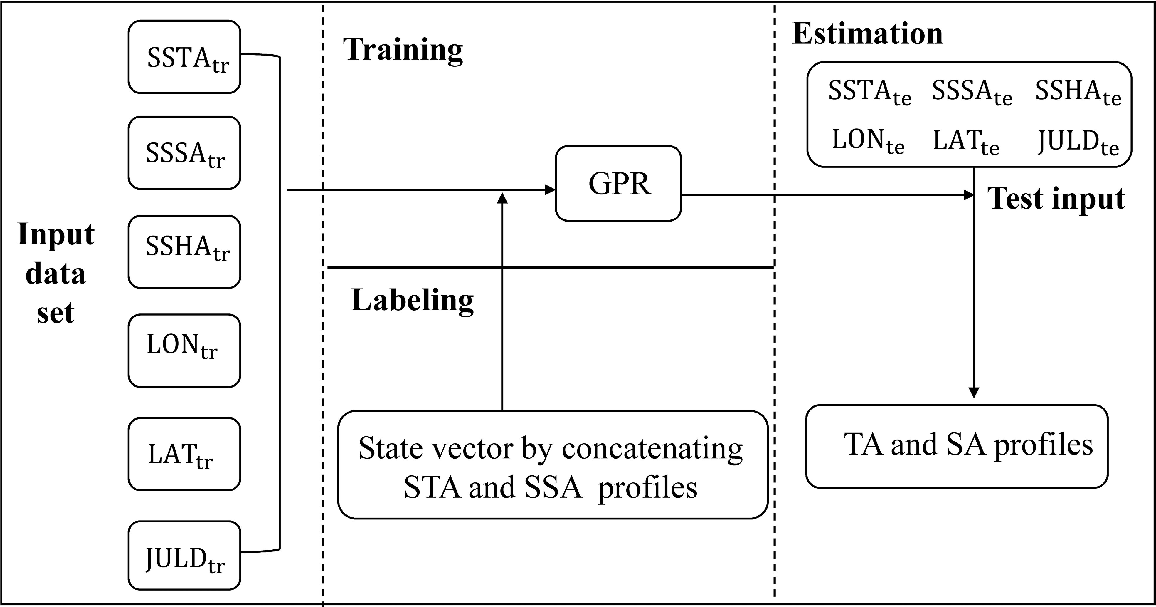
Figure 1 Flowchart of salinity and temperature estimation using GPR.

3.2 Long short-term memory network

LSTM is an extension of the traditional recurrent neural network (RNN), which is mainly used to deal with the case of traditional RNN failure. It solves the problem of gradient disappearance and gradient explosion of traditional RNNs to a certain extent to learn long-term dependent information. Same as general RNN, it also consists of a series of repeating cells with sequential connections, but the structure of the cells is more complex. Crucially, the LSTM adds a state vector updated over time to the cells, which can selectively record the information of the system and preserve the long-term state of the system. Each cell has three inputs, the input $x_i$ of the network at the current time, the output value $h_{i-1}$ at the previous time, and the cell state $C_{i-1}$ at the last time. The input variables are passed through three gates with different functions, namely forget gate, input gate and output gate, to forget and add information to the cell state C_i at the current moment and update the output state $h_i$ at the current moment. The structure of each cell is shown in Figure 2 (Hochreiter and Schmidhuber, 1997), and the tasks of the different gates are implemented using the following equations (Hochreiter and Schmidhuber, 1996; Gers et al., 2000):

FIGURE 2

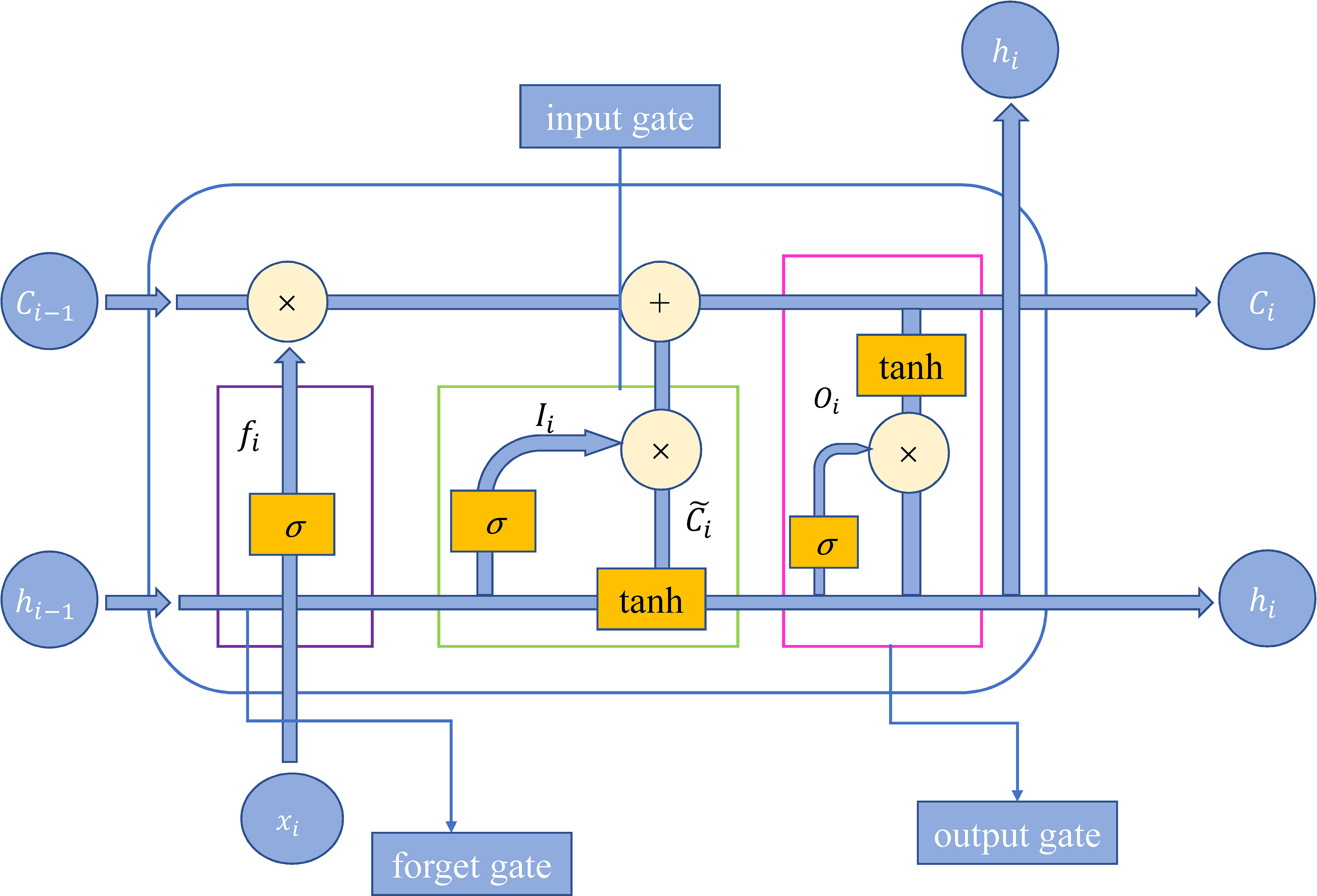
Figure 2 Structure of single cell.

$\begin{array}{ll}\begin{array}{l}{f}_i=\sigma (W_f[h_{i-1},x_i]+b_f),I_i=\sigma (W_I[h_{i-1},x_i]+b_I),\hfill \\ {\tilde{C}}_i=\tanh (W_C[h_{i-1},x_i]+b_C),O_i=\sigma (W_O[h_{i-1},x_i]+b_O),\hfill \\ C_i=f_i*C_{i-1}+I_i*{\tilde{C}}_i,h_i=O_i*\tanh (C_i),\hfill \end{array}& (4)\end{array}$

where $\sigma$ denotes the sigmoid activation function, $W_f,W_I,W_C,W_O$ are weight matrices, $b_f,b_I,b_C,b_O$ are model biases, and $*$ represents dot product operation.

Referring to (Buongiorno Nardelli, 2020), we also use LSTM to estimate the TA and SA profiles. TAs and SAs from different depths are considered the output states of different cells. The input to each cell is the same, a multivariate vector consisting of SSTA, SSSA, SSHA, LON, LAT, and JULD corresponding to the current position. The structure of the LSTM we used is the same as that in (Buongiorno Nardelli, 2020), i.e., a 2-layer stacked network. Each layer contains 35 hidden units, and the optimization algorithm is Adam (Kingma and Ba, 2014). Similarly, we also use max−min normalization to preprocess the data before the LSTM training.

3.3 Proper orthogonal decomposition

POD, which has a wide range of applications in various fields (Liang et al., 2002; Pinnau, 2008; Chapelle et al., 2012; Singler, 2014), provides a means to obtain a low-dimensional description of the system. This method extracts a small number of modes from historical TA and SA profiles that can represent the main features of the field, which simplifies and reduces the dimensionality of the data. The temperature-salinity anomaly profiles at the same location are placed in a multivariate matrix X

$$\mathbf{\text{X}}=\left[\begin{array}{cccc}{T}_{11}& T_{12}& \dots & T_{1n}\\ T_{21}& T_{22}& \dots & T_{2n}\\ \dots & \dots & \dots & \dots \\ T_{m1}& T_{m2}& \dots & T_{mn}\\ S_{11}& S_{12}& \dots & S_{1n}\\ S_{21}& S_{21}& \dots & S_{2n}\\ \dots & \dots & \dots & \dots \\ S_{m1}& S_{m2}& \dots & S_{mn}\end{array}\right]\stackrel{\text{Δ}}{=}[u_1|u_2|\dots |u_n]\in {ℝ}^{2m\times n},$$

where $m$ is the number of vertical levels, $n$ is the number of vertical profiles. In order to calculate the $k$ modes, we only need to do the singular value decomposition of $\mathbf{\text{X}}$ as follows:

$$X=U\text{Σ}{Z}^{\text{T}},$$

where $U\in {ℝ}^{2m\times r}$ and $Z\in {ℝ}^{n\times r}$ are orthogonal matrices. The matrix $\text{Σ}=diag({\sigma }_1,{\sigma }_2,\dots ,{\sigma }_r)$ contains the singular value ${\sigma }_1\ge {\sigma }_2\ge \dots \ge {\sigma }_r$, where $r$ is the rank of $X$. The first $k$ columns of $U$ are the $k$ modes to be computed, which we denote as

$$U_k=U[:,1:k]=\left[\begin{array}{c}{L}_1\\ M_1\end{array}\begin{array}{c}\dots \\ \dots \end{array}\begin{array}{c}{L}_k\\ M_k\end{array}\right].$$

The dimensions of $L_i={[L_{1i},L_{2i},\dots ,L_{mi}]}^{\top }$ and $M_i={[M_{1i},M_{2i},\dots ,M_{mi}]}^{\top }$ is $m\times 1$. Then the corresponding TA profile can be represented by a linear combination of $L_i(i=1,2,\dots ,k)$, and the SA profile is represented by a linear combination of $M_i(i=1,2,\dots ,k)$, where the unknown coefficients are shared. A common method for solving the coefficients is to solve a linear system that is obtained by equating the corresponding sea surface elements inthe reconstructed anomaly profiles to sea surface observations. In this case, $k=2$ is required. To increase $k$, other physical quantities of the ocean need to be added to $X$ to impose constraints on the combined coefficients.

Different from the above methods, in this paper, two methods, GPR and LSTM, are utilized to learn the relationship from the sea surface parameters to the coefficients. In particular, $U_k$ is the solution of the following minimization problem

$\begin{array}{ll}\underset{\mathbf{\text{W}}ϵ{\mathbf{\text{Y}}}_k}{\min }{\Vert \mathbf{\text{X}}-\mathbf{\text{ W}}{\mathbf{\text{W}}}^{\text{T}}\mathbf{\text{X}}\Vert }_F^2 ,& (5)\end{array}$

where ${\mathbf{\text{Y}}}_k=\{\mathbf{\text{W}}\in {ℝ}^{2m\times k}:{\mathbf{\text{W}}}^{\text{T}}\mathbf{\text{W}}={\mathbf{\text{I}}}_k\}$, ${\Vert ·\Vert }_F$ is the Frobenius norm, and the error is estimated as

$\begin{array}{ll}{\Vert \mathbf{\text{X}}-{\mathbf{\text{U}}}_k{\mathbf{\text{U}}}_k^{\text{T}}\mathbf{\text{X}}\Vert }_F^2 =\sum _{i=k+1}^r{\sigma }_i^2.& (6)\end{array}$

From this, we can naturally compute the coefficient vector ${\alpha }_i={\mathbf{\text{U}}}_k^{\text{T}}{u}_i\stackrel{\text{Δ}}{=}{[{\alpha }_i^1,{\alpha }_i^2,\dots ,{\alpha }_i^k]}^{\top }$ corresponding to the historical temperature and salinity anomaly profile $u_i$. And, we can determine $k$ by the following equation according to the required accuracy

$\begin{array}{ll}\frac{{\displaystyle \sum _{i=1}^k{\sigma }_i^2}}{{\displaystyle \sum _{i=1}^r{\sigma }_i^2}}\ge 1-\delta ,& (7)\end{array}$

where $\delta$ is user defined cut-off threshold. To retrieve the vertical structure of TA and SA from the sea surface parameters, we collect the input parameters $x_i$ corresponding to the obtained state vector

$u_i(i=1,2,\dots ,n)$. Here $x_i$ is still a vector consisting of SSTA, SSSA, SSHA, LON, LAT and JULD. Then based on the collected dataset $D_{tr}=\left\{(x_1,{\alpha }_1),(x_2,{\alpha }_2),\dots ,(x_n,{\alpha }_n)\right\}$, we can train GPR or LSTM to build the mapping of input parameters $x$ to coefficients $\alpha$, then the TA and SA are reconstructed as (Hesthaven et al., 2016; Guo and Hesthaven, 2019)

$$\begin{array}{l}T(x)=\sum _{i=1}^k{\alpha }^i(x)L_i,S(x)=\sum _{i=1}^k{\alpha }^i(x)M_i.\hfill \end{array}$$

The corresponding flow chart is given in Figure 3.

FIGURE 3

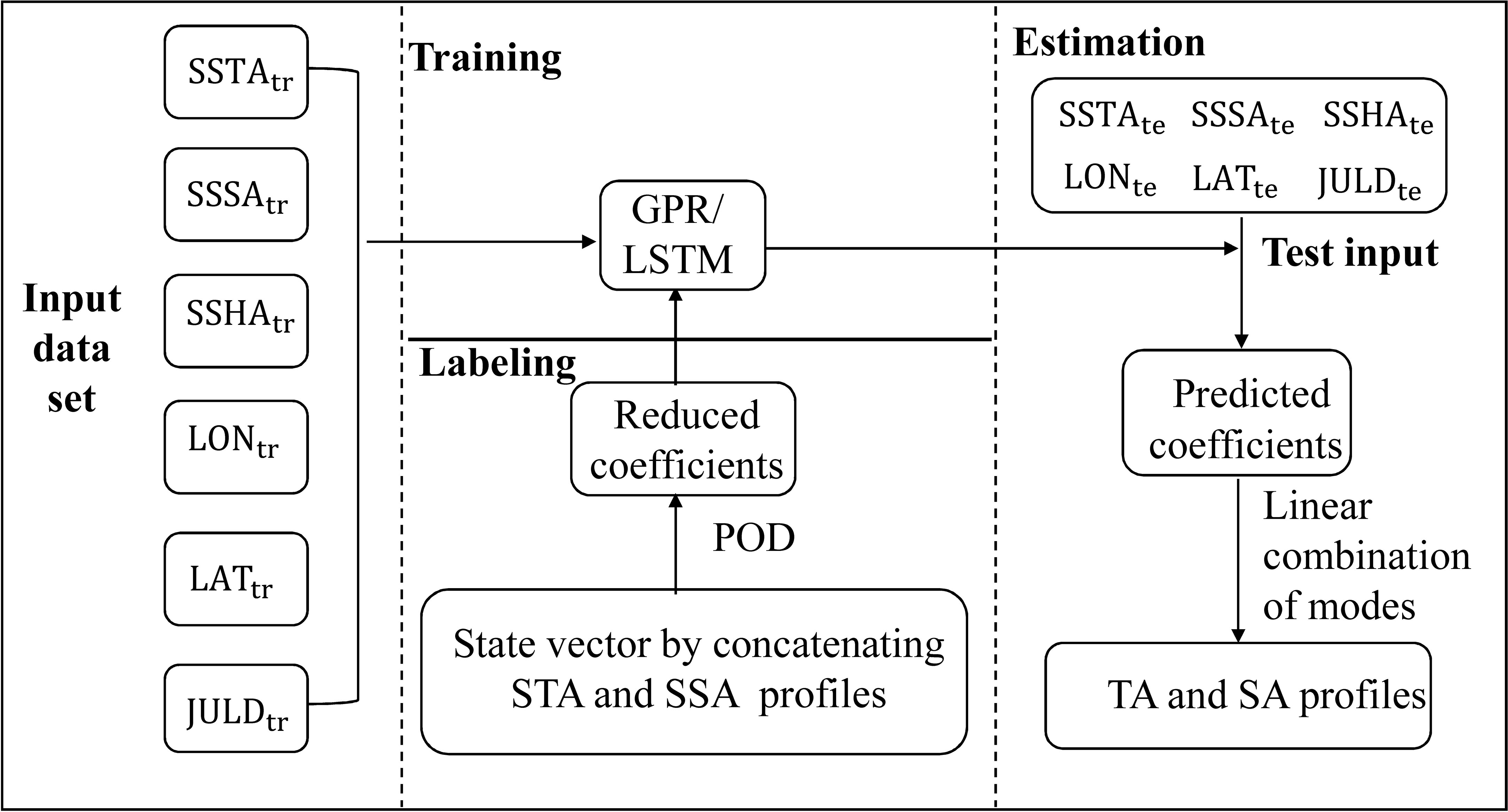
Figure 3 Flowchart of salinity and temperature estimation using GPR-POD and LSTM-POD.

Further, we point out that $L_i$ and $M_i$ are actually functions of depth $z$. To estimate the TA and SA at any depth $z^{*}$, we use cubic spline interpolation to interpolate $L_i$ and $M_i$ with respect to depth $z$ to obtain the corresponding interpolation functions ${\tilde{L}}_i(z)$ and ${\tilde{M}}_i(z)$ satisfying ${\tilde{L}}_i(z_j)=L_{ji}$ and ${\tilde{M}}_i(z_j)=M_{ji}(i=1,2,\dots ,k,j=1,2,\dots ,,m)$, where $z_i(i=1,2,\dots ,m)$ denotes the vertical levels, so that the TA and SA at depth $z^{*}$ can be reconstructed as

$$\begin{array}{l}T(z^{*},x)=\sum _{i=1}^k{\alpha }^i(x){\tilde{L}}_i(z^{*}),S(z^{*},x)=\sum _{i=1}^k{\alpha }^i(x){\tilde{M}}_i(z^{*}).\hfill \end{array}$$

4 Results

4.1 Comparison between different models

To evaluate the performance of different models, we randomly selected 20% of the 11,374 Argo profiles as the test set and the remaining 80% as the training set. Different models are then employed to retrieve TA and SA profiles with the same inputs, i.e., SSTA, SSSA, SSHA, LON, LAT, and JULD. The RMSE between TA and SA profiles obtained from these models and the Argo profiles is calculated to evaluate the performance of the different methods. The RMSE of the WOA is obtained by comparing the temperature and salinity profiles obtained after interpolating the monthly mean of the climatology of WOA18 with the Argo profiles. Let δ=0.04% and we choose k=14 modes, in fact, before performing the POD, we similarly scaled the data between 0 and 1. Figure 4 shows the vertical distribution of the RMSEs estimated by the different models. The RMSEs of all proposed methods are smaller than the RMSE of the WOA18, and a similar vertical structure can be seen in the different models. The RMSEs are small at the sea surface but increase rapidly with depth, decrease rapidly after reaching the maximum, and stabilized. This may be related to the complex dynamical processes in the ocean’s upper layers and the perturbations in the mixed and thermocline layers, while the seawater is relatively stable in the deeper layers. The RMSEs of temperature reach their maximum at 105 - 115 m, and only near this depth (where the temperature variation is relatively large), LSTM shows superior performance in predicting TA profiles compared to other methods. This suggests that LSTM may have greater potential for approximating strongly nonlinear functions since, at depths where temperature changes rapidly, the relationship between temperature and depth is more complex and may have stronger nonlinearity.

FIGURE 4

Figure 4 Estimated RMSEs of different models. (A) RMSEs of estimated temperature. (B) RMSEs of estimated salinity.

However, the performance of the four methods is comparable from an overall perspective. The RMSEs of salinity reach their maximum between 55 - 65 m. Although the four reconstruction methods have comparable accuracy, GPR performs a little better than LSTM in the reconstruction of upper salinity, which may arise because the rate of change of the salinity profile is not as large as that of the temperature profile, GPR can produce sufficiently accurate approximations, while LSTM has a more complex structure and numerous parameters, making them reliant on large amounts of training data to obtain more accurate predictions. In addition, the POD combined with the regression methods does not cause a large loss in the accuracy of the estimated profiles, which is better reflected in the RMSEs of GPR and GPR-POD, as the RMSEs of both are almost the same. The selected modes are sufficient to characterize the vast majority of the temperature and salinity fields. To further measure the uncertainty of the estimates of GPR-based methods, Figure 5 shows the standard deviation of the posterior distribution of the GPR and GPR-POD predictions. We can see that both methods display similar distribution patterns, with comparable uncertainty estimates at most points, but the uncertainty of the model prediction is higher at the western boundary of the region, which can be attributed to the limited training data available in this region. This also shows a drawback of the GPR-based approach, which is better suited for interpolated predictions rather than extrapolation. Notably, the predictions of GPR-POD exhibit higher levels of uncertainty, despite comparable RMSEs between GPR-POD and GPR. This discrepancy may be attributed to the fact that more information is available in the training data for GPR, making it more confident in its predictions.

FIGURE 5

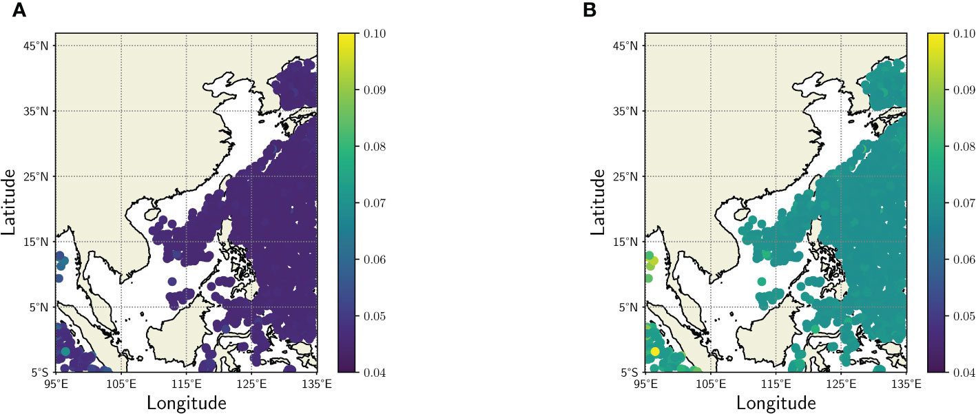
Figure 5 Uncertainty estimation of (A) GPR and (B) GPR-POD.

Considering the inhomogeneity and sparsity of spatio-temporal distribution of thermohaline data, all the thermohaline relationships in the test set are drawn in the same graph (Figure 6), the purpose of which is to compare the predictions of different models, in which the different colors of points are to better distinguish the differences between points. The main distribution structure of T-S graph reconstructed by all methods is similar to that of Argo field, but the distribution range of points is more concentrated than that of Argo field. From the T-S graphs, it can be observed that the reconstructed results are generally weaker for the points with larger absolute values of salinity anomalies. To better visualize the predicted distribution of temperature and salinity anomalies, a histogram of the number of salinity anomalies in different intervals is displayed at the top of the T-S graph, and a histogram of temperature anomalies is displayed on the right side of the T-S graph. The histogram of salinity anomalies reveals that the distribution of LSTM-POD is more consistent with that of Argo, while LSTM underestimates the number of points of salinity anomalies in the interval [-0.5,0], which is overestimated by GPR and GPR-POD. The histograms of temperature anomalies from different models indicate that all four methods overestimate the number of temperature anomalies in the interval [0,2.5], but their overall distribution is very similar to that of Argo. In conclusion, the reconstructed methods can predict the main distribution structure of the T-S graph. Although there are slight differences in the distribution range and there may be problems of underestimating the thermohaline state, the performance of the proposed reconstructed methods is generally satisfactory. Furthermore, Figure 7 displays the scatter plots of the LSTM estimated and Argo’s temperature and salinity anomalies at a depth of 105 m. This depth is significantly impacted by the variation of the upper mixed layer, and the RMSE estimated for temperature and salinity at this depth is also large. The results indicate that the overall discrepancy between them is minimal, as the LSTM prediction preserves the fundamental characteristics of the temperature and salinity anomalies, and its pattern (positive or negative) is accurately reconstructed.

FIGURE 6

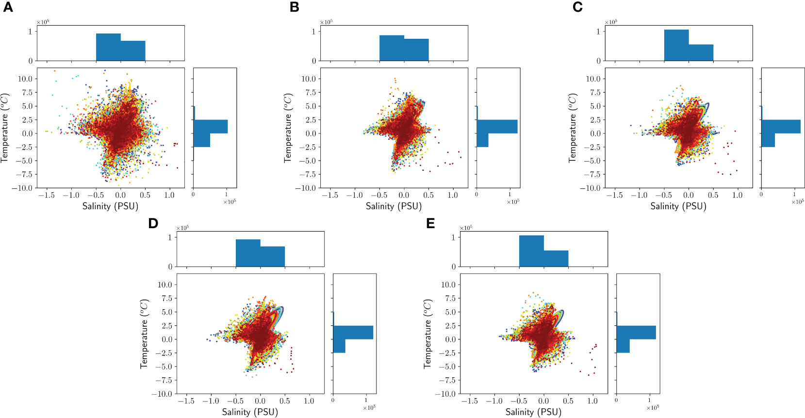
Figure 6 T-S graph and histogram of temperature and salinity anomalies for different models. (A) T-S graph for Agro (left and bottom), histogram of the number of salinity anomalies in different intervals for Agro (top), histogram of the number of temperature anomalies in different intervals for Agro (right). Panels (B-E) are the same as panels (A), respectively, except for (B) LSTM, for (C) GPR, for (D) LSTM-POD and for (E) GPR-POD.

FIGURE 7

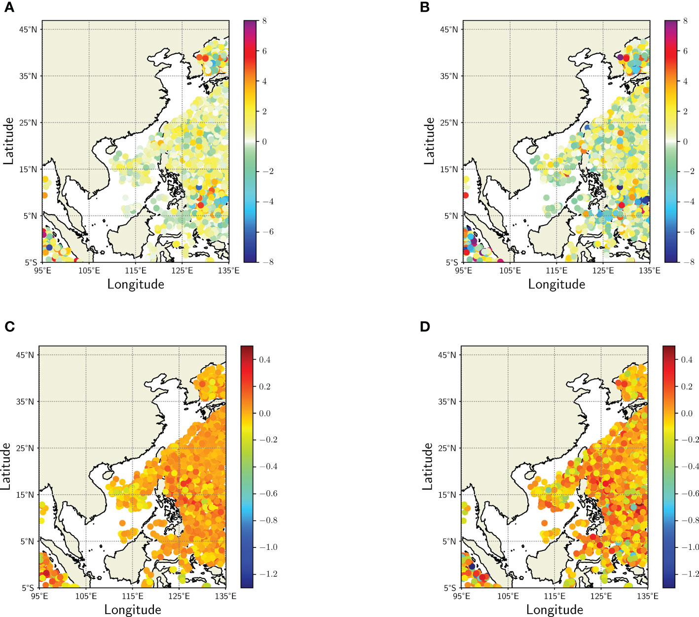
Figure 7 TAs and SAs of different models at 105 m. (A) LSTM-estimated TAs. (B) Argo TAs. (C) LSTM-estimated SAs. (D) Argo SAs.

To further compare the improvement of POD on the computational efficiency of different models, we compare the running times of different models. The CPU times of LSTM and LSTM-POD are 11216 s and 1488 s, respectively, computed using a laptop with 4 Intel(R) Core(TM) i7-6770 CPU @ 3.40GHz and 8G Memory. Since GPR requires higher memory for matrix operations, GPR and GPR-POD are run using a single node with a single core in Tianhe-2, which adopts an Intel Xeon E5-2692 v2 CPU @ 2.20GHz and 64GB Memory. Furthermore, the running times of GPR and GPR-POD are 891 s and 788 s, respectively. We can see that the training time of LSTM can be significantly reduced by combining POD, as LSTM takes 7.5 times longer than LSTM-POD. However, this reduction is not apparent in GPR, this is attributed to the fact that the computational complexity of GPR-POD is ${\rm O}(k{n}^3)$, while the computational complexity of GPR is ${\rm O}(2m{n}^3)$. In this case, n=9099,k=14,m=71, the improvement in training time is insignificant when the number of training samples is much larger than the number of output dimensions.

4.2 Sensitivity of different parameters in GPR-POD

To test the sensitivity of the estimated TA and SA to different input parameters, we compare GPR-POD estimates with different training inputs. Figure 8. shows the RMSEs of temperature with various inputs, and as well as the correlation between test input parameters, the correlation between test input parameters, and test TA profiles , and the correlation between test input parameters and test SA profiles. By observing the RMSEs of temperature, we can find that the RMSE of the model without SSHA in the input is large at all depths, which indicates that SSHA plays a vital role in ocean motion and processes. In fact, changes in the subsurface layer may give rise to changes in SSH resulting from the interaction of several factors, such as heat exchange, internal thermal expansion, and ocean circulation. A rise in sea temperature leads to an increase in SSH, while a decrease in sea temperature leads to a reduction in SSH. The correlation coefficients between SSHA and TA profiles also affirm the excellent association between SSHA and TA. Notably, the correlation coefficient between SSHA and TA is the highest among all input parameters except SSTA. In addition, SSH changes under the influence of wave and wind shear. Incorporating SSHA into the model input can provide more information for predicting TA. Latitude, longitude, and time all improve the TA profile reconstruction to different degrees, showing that geographic and temporal information is helpful in predicting TA. In particular, incorporating latitude data yields a more substantial reduction in RMSE than incorporating longitude data, suggesting that latitude has a greater impact on TA reconstruction. This is because the discrepancy in solar radiation across different latitudes results in significant variations in sea temperature in the north-south direction. Therefore, latitude information is essential to improve the performance of subsurface reconstruction. Furthermore, the correlation between latitude and TA profiles is higher compared to that between longitude and TA profiles, highlighting the importance of considering latitude when predicting TA. The model without SSTA in the input has the largest RMSE in the upper layer (<100 m ), but when the depth is greater than 100 m, there is almost no difference between the model without SSTA and GPR-POD ( all parameters as input). This suggests that SSTA data mainly improve the reconstruction of upper layer TA, while deeper temperature variations are difficult to be interpreted from satellite measurements. In addition to the fact that SSSA has no significant relationship with ocean interior temperature, which can also be verified by observing the correlation between SSSA and TA profiles. Similar results can be observed in the RMSEs of salinity, where adding both latitude and SSHA data reduces the RMSEs of salinity at all depths. The relationship between ocean salinity and temperature on density is a fundamental aspect that affects changes in SSH, causing SSHA and SA profiles to have some correlation. Latitude also influences changes in ocean salinity as a result of a combination of factors, including precipitation, evaporation, and mixing of water masses. Consequently, incorporating latitude and SSHA into the prediction of subsurface salinity can significantly improve model accuracy. SSSA data play an important role in the reconstruction of upper ocean SA profiles, while they do not help much in the reconstruction of deep SA profiles, and the correlation between SSSA and SA gradually decreased with increasing depth. The RMSEs of several other models show that longitude, time, and SSTA have somewhat limited improvements on the models, where longitude and time can reduce the maximum of salinity RMSE, while SSTA has no significant improvement on the reconstruction of SA profiles.

FIGURE 8

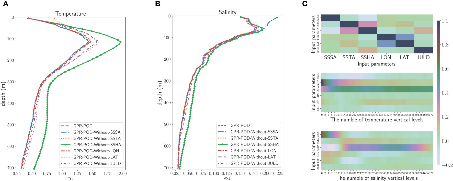
Figure 8 (A) RMSEs of temperature from models with different sea surface inputs. (B) RMSEs of salinity from models with different sea surface inputs. (C) heat map of correlation coefficients.

4.3 The performance of climatology on three-dimensional salinity and temperature fields reconstruction

To test the influence of climatology on the temperature and salinity reconstruction models, we considered three different inputs and outputs for LSTM and GPR. The inputs are 1) X: SSTA, SSSA, SSHA, LAT, LON, JULD; 2) X-Without-WOA: SST, SSS, SSHA, LAT, LON, JULD, and 3) X-WOA: SST, SSS, SSHA, LAT, LON, JULD, SS (climatology), ST (climatology) and the outputs are 1) X: STA, SSA; 2) X-Without-WOA: SS, ST, and 3) X-WOA: SS, ST. The RMSEs estimated by different models are shown in Figure 9. Observing the RMSEs of the two regression models with various inputs and outputs, we can find a similar behavior, especially when the temperature at depths of less than 100 m and the salinity at depths of less than 200 m, training the models with the temperature and salinity anomaly fields can significantly improve the prediction accuracy than directly using temperature and salinity as the input and output of the model. This is because the seasonal variation signal disappears after calculating the anomaly field using the monthly mean of climatology, thus making the SS and SA easier to predict. On the other hand, incorporating monthly temperature and salinity climatology fields into the model input gives the most accurate estimates. Climatological information added to the input can effectively reduce the impact of the sea surface parameter errors. In summary, seasonal variations in seawater temperature and salinity play a crucial role in oceanic processes. The information provided by seasonal variations in temperature and salinity can help us better estimate temperature and salinity structure within the ocean.

FIGURE 9

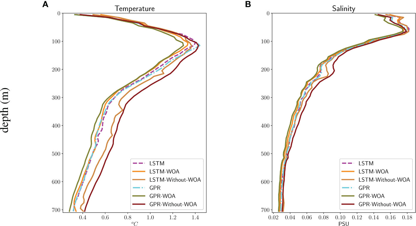
Figure 9 The RMSEs of temperature and salinity from models with different inputs and outputs. (A) RMSEs of estimated temperature. (B) RMSEs of estimated salinity.

Comparing LSTM and GPR with the same input and output, it can be found that the accuracy of GPR with temperature and salinity climatology as input is higher than that of LSTM. This is due to the inclusion of monthly climate fields of temperature and salinity in the input, which makes the model less complex. Similar to the findings in Section 4.1, GPR can provide more accurate predictions when the amount of training data is not abundant. In contrast, the performance of GPR without considering climatology is the worst, expressly, by up to 20% (∼245 m) over the GPR-WOA estimate. When only sea surface parameters are included in the input without climatology as an aid, it leads to a more complex relationship between the input and output in the model. The LSTM, on the other hand, can better approximate the strongly nonlinear function, so the GPR-Without-WOA does not perform as well as the LSTM-Without-WOA.

4.4 Estimation of temperature and salinity using continuous remote sensing data from SSHA and SSTA

Since the SSS data is the 4-day temporal grid, in order to make full use of the other daily satellite and in situ observations, we use the SSTA, SSHA, LAT, LON, and JULD as model inputs in this section to train the LSTM model (named LSTM-Daily) to estimate the TA and SA profiles. Thus, there are 45,031 Argo observation profiles available, and again, 80% are randomly selected as the training set, and the remaining 20% are used to test the model’s performance. The RMSEs of the temperature and salinity estimated by LSTM-Daily are shown in Figure 10, respectively, besides the RMSE reduction rate of LSTM relative to climatological estimates also shown in Figure 10. It is clear that the RMSE of the estimated TA profiles is reduced by 20%−70% compared to climatology. By increasing the training data size, a more accurate reconstruction of the temperature profiles can be obtained. On the other hand, the prediction accuracy decreases for salinity at depths less than 100 due to the lack of SSS information, which again validates the importance of SSSA for SA reconstruction at a depth of less than 100 m. However, when the depth is greater than 100 m, as the effect of SSSA data disappears, higher accuracy SA estimation can be achieved again due to increased training data size.

FIGURE 10

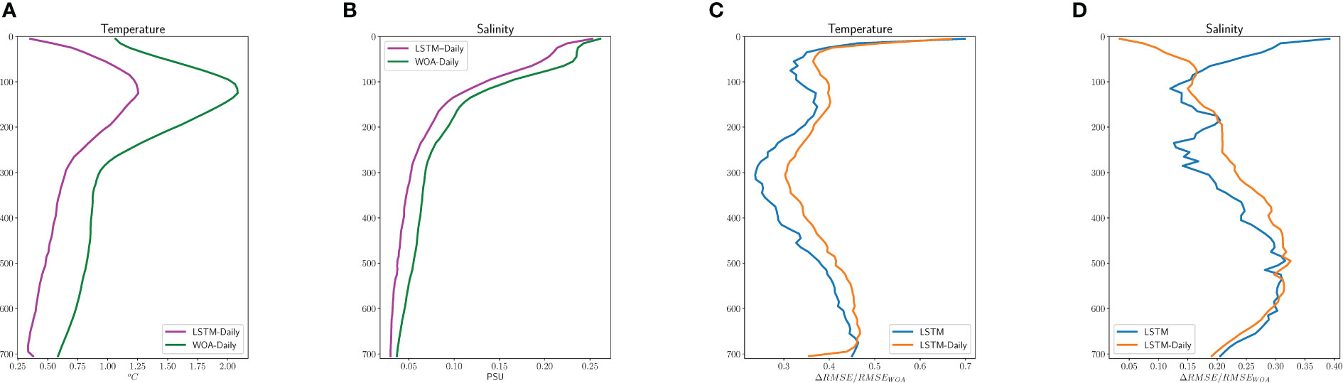
Figure 10 The RMSEs of estimated temperature and salinity, and the reduction of RMSE for LSTM reconstructed profiles relative to climatological profiles. (A) RMSEs of estimated temperature. (B) RMSEs of estimated salinity. (C) The reduction of temperature’s RMSE. (D) The reduction of salinity’s RMSE.

5 Discussion

This paper applies several methods to estimate the TA and SA profiles from sea surface parameters, namely LSTM, GPR, LSTM-POD, and GPR-POD. LSTM and GPR directly train the model with TAs and SAs at different depths as the output. At the same time, LSTM-POD and GPR-POD combine LSTM, GPR respectively, with POD, which can downscale the data, and it assumes that only a small number of modes are needed to represent the main features of the temperature and salinity anomaly fields. Thus, only the model needs to be trained to estimate the coefficients, i.e., the output of the model is the reduced coefficients corresponding to the temperature-salinity anomaly profiles, which greatly simplifies the regression model. In addition, using the predicted coefficients, a linear combination of the interpolated modes can estimate TA and SA at any depth. We selected Argo observations and satellite remote sensing data for the Northwest Pacific Ocean in 2011-2021 for training and testing. The accuracy and reliability of the proposed methods are evaluated by calculating the RMSEs of the estimated profiles, and the results show that these methods can accurately derive the TA and SA profiles, and the introduction of POD greatly saves time and storage costs without additional loss of accuracy, especially for LSTM.

In order to determine the relative importance of different input parameters to the temperature and salinity reconstruction, we evaluate the results of several models with different inputs, in addition to which correlations between different parameters and TA and SA profiles are calculated. The results show that the most significant improvements can be obtained by including SSHA and latitude. On the other hand, SSTA and SSSA play an important role in the TA and SA reconstruction in the upper layers (>100 m), but this role decreases with increasing depth. In addition, by using the temperature and salinity monthly climatological fields, especially when added to the input of the regression model, fairly good profile predictions can be obtained, both for LSTM and GPR. This suggests that the introduction of climatology can effectively reduce the effect of sea surface errors and provide more information to the regression model, thus effectively improving the accuracy and robustness of the model. This also inspires us to explore multiple satellite measurements further to improve the reliability of the estimates in the future.

In general, the proposed methods can be effectively used for reconstructing temperature and salinity profiles, particularly when monthly climatology of temperature and salinity is included as an input to the GPR. The techniques presented in this article for estimating subsurface temperature and salinity do not require any prior knowledge or assumptions and are highly versatile and generalized. These models can accurately predict new subsurface temperature and salinity values as long as it is well-trained. It is expected that the proposed methods can be beneficial for the detection of the thermal structure of the ocean interior in marine science and climate change research, as well as for more precise analysis of temperature and salinity changes. However, it is important to note that, unlike dynamic-based reconstruction methods, the proposed methods are solely based on data and lack of physical interpretation, which may be a limitation in the development of artificial intelligence approaches to oceanography. With the rapid advancement of ocean modeling capability, observation technology and artificial intelligence, it is a promising direction to effectively combine the advantages of a dynamics-based approach and data-driven approach in future work, enhance the ability of model prediction and physical interpretation, and establish a deep learning model based on physical information.

Data availability statement

The original contributions presented in the study are included in the article/supplementary material. Further inquiries can be directed to the corresponding author.

Author contributions

YC: Methodology, Investigation, Performer Experiment, Writing Original Draft. LL: Data Collection and Curation, Writing-Review. XC: Formal Analysis, Writing-Review and Editing. ZW: Supervision, Writing-Reviewing. XS: Writing-Review and Editing. CY: Writing-Review and Editing. ZG: Writing-Review, Project Administration, Funding Acquisition. All authors contributed to the article and approved the submitted version.

Funding

This study was supported by the National Key Research and Development Program of China (2021YFF0704000), the Taishan Scholars Progam (tsqn202211059) and the Fundamental Research Funds for the Central Universities (202265005, 202264007).

Acknowledgments

The authors would like to thank the reviewers for their valuable suggestions on the manuscript.

Conflict of interest

The authors declare that the research was conducted in the absence of any commercial or financial relationships that could be construed as a potential conflict of interest.

The reviewer XL declared a shared affiliation with the authors to the handling editor at the time of review.

Publisher’s note

All claims expressed in this article are solely those of the authors and do not necessarily represent those of their affiliated organizations, or those of the publisher, the editors and the reviewers. Any product that may be evaluated in this article, or claim that may be made by its manufacturer, is not guaranteed or endorsed by the publisher.

References

Ali M., Swain D., Weller R. A. (2004). Estimation of ocean subsurface thermal structure from surface parameters: a neural network approach. Geophysical Res. Lett. 31, L20308. doi: 10.1029/2004GL021192

CrossRef Full Text | Google Scholar

Ballabrera-Poy J., Mourre B., Garcia-Ladona E., Turiel A., Font J. (2009). Linear and non-linear t–s models for the eastern north atlantic from argo data: role of surface salinity observations. Deep Sea Res. Part I: Oceanographic Res. Papers 56, 1605–1614. doi: 10.1016/j.dsr.2009.05.017

CrossRef Full Text | Google Scholar

Bao S., Ren Z., Wang H., Yan H., Yu Y., Chen J. (2018). Salinity profile estimation in the pacific ocean from satellite surface salinity observations. J. Atmospheric Oceanic Technol. 36, 53–68. doi: 10.1175/JTECH-D-17-0226.1

CrossRef Full Text | Google Scholar

Boyer T. P., Garcia H. E., Locarnini R. A., Zweng M. M., Mishonov A. V., Reagan J. R., et al. (2018). World ocean atlas 2018. (United States: NOAA National Centers for Environmental Information). Dataset. Available at: https://www.ncei.noaa.gov/archive/accession/NCEI-WOA18.

Google Scholar

Buongiorno Nardelli B. (2020). A deep learning network to retrieve ocean hydrographic profiles from combined satellite and in situ measurements. Remote Sens. 12, 3151. doi: 10.3390/rs12193151

CrossRef Full Text | Google Scholar

Buongiorno Nardelli B., Santoleri R. (2005). Methods for the reconstruction of vertical profiles from surface data: multivariate analyses, residual gem, and variable temporal signals in the north pacific ocean. J. Atmospheric Oceanic Technol. 22, 1763–1781. doi: 10.1175/JTECH1792.1

CrossRef Full Text | Google Scholar

Carnes M. R., Mitchell J. L., de Witt P. W. (1990). Synthetic temperature profiles derived from geosat altimetry: comparison with air-dropped expendable bathythermograph profiles. J. Geophysical Research: Oceans 95, 17979–17992. doi: 10.1029/JC095iC10p17979

CrossRef Full Text | Google Scholar

Carnes M. R., Teague W. J., Mitchell J. L. (1994). Inference of subsurface thermohaline structure from fields measurable by satellite. J. Atmospheric Oceanic Technol. 11551–566. doi: 10.1175/1520-0426(1994)011<0551:IOSTSF>2.0.CO;2

CrossRef Full Text | Google Scholar

Carrassi A., Bocquet M., Bertino L., Evensen G. (2018). Data assimilation in the geosciences: an overview of methods, issues, and perspectives. Wiley Interdiscip. Reviews: Climate Change 9, e535. doi: 10.1002/wcc.535

CrossRef Full Text | Google Scholar

Chapelle D., Gariah A., Sainte-Marie J. (2012). Galerkin approximation with proper orthogonal decomposition : new error estimates and illustrative examples. ESAIM: Math. Model. Numerical Anal. 46, 731–757. doi: 10.1051/m2an/2011053

CrossRef Full Text | Google Scholar

Chen Z., Wang X., Liu L. (2020). Reconstruction of three-dimensional ocean structure from Sea surface data: an application of isQG method in the southwest Indian ocean. J. Geophysical Res. (Oceans) 125, e2020JC016351. doi: 10.1029/2020JC016351

CrossRef Full Text | Google Scholar

Chen C., Yang K., Ma Y., Wang Y. (2018). Reconstructing the subsurface temperature field by using sea surface data through self-organizing map method. IEEE Geosci. Remote Sens. Lett. 15, 1812–1816. doi: 10.1109/LGRS.2018.2866237

CrossRef Full Text | Google Scholar

de Boyer Montégut C., Mignot J., Lazar A., Cravatte S. (2007). Control of salinity on the mixed layer depth in the world ocean: 1. general description. J. Geophysical Research: Oceans 112, C06011. doi: 10.1029/2006JC003953

CrossRef Full Text | Google Scholar

Fiedler P. (1988). Surface manifestations of subsurface thermal structure in the california current. J. Geophysical Res. 93, 4975–4983. doi: 10.1029/JC093iC05p04975

CrossRef Full Text | Google Scholar

Forrester A. I., Sóbester A., Keane A. J. (2008). Engineering Design via Surrogate Modelling: A Practical Guide. (Chichester, UK: John Wiley & Sons Ltd.) doi: 10.1002/9780470770801

CrossRef Full Text | Google Scholar

Fujii Y., Kamachi M. (2003a). A reconstruction of observed profiles in the sea east of japan using vertical coupled temperature-salinity eof modes. J. Oceanography 59, 173–186. doi: 10.1023/A:1025539104750

CrossRef Full Text | Google Scholar

Fujii Y., Kamachi M. (2003b). Three-dimensional analysis of temperature and salinity in the equatorial pacific using a variational method with vertical coupled temperature-salinity empirical orthogonal function modes. J. Geophysical Research: Oceans 108, 3297. doi: 10.1029/2002JC001745

CrossRef Full Text | Google Scholar

Gers F. A., Schmidhuber J., Cummins F. (2000). Learning to forget: continual prediction with LSTM. Neural Comput. 12, 2451–2471. doi: 10.1162/089976600300015015

PubMed Abstract | CrossRef Full Text | Google Scholar

Ghil M., Malanotte-Rizzoli P. (1991). Data Assimilation in Meteorology and Oceanography. (Elsevier) Adv. Geophysics. 33, 141–266. doi: 10.1016/S0065-2687(08)60442-2

CrossRef Full Text | Google Scholar

GPy (2012). Gpy: a gaussian process framework in python. (Sheffield, UK: The University of Sheffield)

Google Scholar

Guinehut S., Dhomps A.-L., Gilles L., Traon P.-Y. (2012). High resolution 3-d temperature and salinity fields derived from in situ and satellite observations. Ocean Sci. Discussions 9, 1313–1347. doi: 10.5194/osd-9-1313-2012

CrossRef Full Text | Google Scholar

Guo M., Hesthaven J. S. (2019). Data-driven reduced order modeling for time-dependent problems. Comput. Methods Appl. Mechanics Eng. 345, 75–99. doi: 10.1016/j.cma.2018.10.029

CrossRef Full Text | Google Scholar

Helber R., Richman J., Barron C. (2010). The influence of temperature and salinity variability on the upper ocean density and mixed layer. Ocean Sci. Discussions (OSD) 7, 1469–1495. doi: 10.5194/osd-7-1469-2010

CrossRef Full Text | Google Scholar

Held I. M., Pierrehumbert R. T., Garner S. T., Swanson K. L. (1995). Surface quasi-geostrophic dynamics. J. Fluid Mechanics 282, 1–20. doi: 10.1017/S0022112095000012

CrossRef Full Text | Google Scholar

Hesthaven J., Rozza G., Stamm B. (2016). Certified reduced basis methods for parametrized partial differential equations. (Switzerland: Springer) doi: 10.1007/978-3-319-22470-1

CrossRef Full Text | Google Scholar

Hochreiter S., Schmidhuber J. (1996). “LSTM can solve hard long time lag problems,” in Proceedings of the 9th international conference on neural information processing systems, vol. NIPS’96. (Cambridge, MA, USA: MIT Press), 473–479.

Google Scholar

Hochreiter S., Schmidhuber J. (1997). Long short-term memory. Neural Comput. 9, 1735–1780. doi: 10.1162/neco.1997.9.8.1735

PubMed Abstract | CrossRef Full Text | Google Scholar

Isern-Fontanet J., Chapron B., Lapeyre G., Klein P. (2006). Potential use of microwave sea surface temperatures for the estimation of ocean currents. Geophysical Res. Lett. 33, OS14B–OS101. doi: 10.1029/2006GL027801

CrossRef Full Text | Google Scholar

Isern-Fontanet J., Lapeyre G., Klein P., Chapron B., Hecht M. W. (2008). Three-dimensional reconstruction of oceanic mesoscale currents from surface information. J. Geophysical Research: Oceans 113, C09005. doi: 10.1029/2007JC004692

CrossRef Full Text | Google Scholar

Kingma D., Ba J. (2014). Adam: A method for stochastic optimization. (San Diego: 3rd International Conference for Learning Representations). arXiv preprint arXiv:1412.6980

Google Scholar

Klemas V., Yan X.-H. (2014). Subsurface and deeper ocean remote sensing from satellites: an overview and new results. Prog. Oceanography 122, 1–9. doi: 10.1016/j.pocean.2013.11.010

CrossRef Full Text | Google Scholar

Klemas V., Yan X.-H. (2014). Subsurface and deeper ocean remote sensing from satellites: An overview and new results. Progress in Oceanography 122, 1–9. doi: 10.1016/j.pocean.2013.11.010

CrossRef Full Text | Google Scholar

Lapeyre G., Klein P. (2006). Dynamics of the upper oceanic layers in terms of surface quasigeostrophy theory. J. Phys. Oceanography 36, 165–176. doi: 10.1175/JPO2840.1

CrossRef Full Text | Google Scholar

Li W., Su H., Wang X., Yan X. (2017). Estimation of global subsurface temperature anomaly based on multisource satellite observations. J. Remote Sens. 21, 881–891. doi: 10.11834/jrs.20177026

CrossRef Full Text | Google Scholar

Liang Y., Lee H., Lim S., Lin W., Lee K., Wu C. (2002). Proper orthogonal decomposition and its applications - part I: theory. J. Sound Vibration 252, 527–544. doi: 10.1006/jsvi.2001.4041

CrossRef Full Text | Google Scholar

Liu Z., Li Z., Lu S., Wu X., Sun C., Xu J. (2021). Scattered dataset of global ocean temperature and salinity profiles from the international argo program. J. Global Change Data Discovery 5, 312–321. doi: 10.3974/geodp.2021.03.09

CrossRef Full Text | Google Scholar

Liu L., Peng S., Huang R. X. (2017). Reconstruction of ocean’s interior from observed sea surface information. J. Geophysical Research: Oceans 122, 1042–1056. doi: 10.1002/2016JC011927

CrossRef Full Text | Google Scholar

Liu L., Peng S., Wang J., Huang R. X. (2014). Retrieving density and velocity fields of the ocean’s interior from surface data. J. Geophysical Research: Oceans 119, 8512–8529. doi: 10.1002/2014JC010221

CrossRef Full Text | Google Scholar

Liu L., Xue H., Sasaki H. (2019). Reconstructing the ocean interior from high-resolution Sea surface information. J. Phys. Oceanography 49, 3245–3262. doi: 10.1175/JPO-D-19-0118.1

CrossRef Full Text | Google Scholar

Lu W., Su H., Yang X., Yan X.-H. (2019). Subsurface temperature estimation from remote sensing data using a clustering-neural network method. Remote Sens. Environ. 422, 213–222. doi: 10.1016/j.rse.2019.04.009

CrossRef Full Text | Google Scholar

Lucia D. J., Beran P. S., Silva W. A. (2004). Reduced-order modeling: new approaches for computational physics. Prog. Aerospace Sci. 40, 51–117. doi: 10.1016/j.paerosci.2003.12.001

CrossRef Full Text | Google Scholar

Maes C., Behringer D., Reynolds R., Ji M. (2000). Retrospective analysis of the salinity variability in the western tropical pacific ocean using an indirect minimization approach. J. Atmospheric Oceanic Technol. 17, 512–524. doi: 10.1175/1520-0426(2000)017<0512:RAOTSV>2.0.CO;2

CrossRef Full Text | Google Scholar

Masuko T. (2017). “Computational cost reduction of long short-term memory based on simultaneous compression of input and hidden state,” in 2017 IEEE automatic speech recognition and understanding workshop (ASRU) (Piscataway, New Jersey, USA: IEEE), 126–133. doi: 10.1109/ASRU.2017.8268926

CrossRef Full Text | Google Scholar

Meehl G. A., Arblaster J. M., Fasullo J. T., Hu A., Trenberth K. E. (2011). Model-based evidence of deep-ocean heat uptake during surface-temperature hiatus periods. Nat. Climate Change 1, 360–364. doi: 10.1038/nclimate1229

CrossRef Full Text | Google Scholar

Meinen C. S., Watts D. R. (2000). Vertical structure and transport on a transect across the north atlantic current near 42° n: time series and mean. J. Geophysical Research: Oceans 105, 21869–21891. doi: 10.1029/2000JC900097

CrossRef Full Text | Google Scholar

Melnichenko O., Hacker P., Maximenko N., Lagerloef G., Potemra J. (2016). Optimum interpolation analysis of aquarius sea surface salinity. J. Geophysical Research: Oceans 121, 602–616. doi: 10.1002/2015JC011343

CrossRef Full Text | Google Scholar

Meng L., Yan X.-H. (2022). Remote sensing for subsurface and deeper oceans: an overview and a future outlook. IEEE Geosci. Remote Sens. Magazine 10, 72–92. doi: 10.1109/MGRS.2022.3184951

CrossRef Full Text | Google Scholar

Moore A., Martin M., Akella S., Arango H., Balmaseda M., Bertino L., et al. (2019). Synthesis of ocean observations using data assimilation for operational, real-time and reanalysis systems: a more complete picture of the state of the ocean. Front. Mar. Sci. 6. doi: 10.3389/fmars.2019.00090

CrossRef Full Text | Google Scholar

Nardelli B. B., Santoleri R. (2004). Reconstructing synthetic profiles from surface data. J. Atmospheric Oceanic Technol. 21, 693–703. doi: 10.1175/1520-0426(2004)021<0693:RSPFSD>2.0.CO;2

CrossRef Full Text | Google Scholar

Nguyen N., Peraire J. (2016). Gaussian Functional regression for output prediction: model assimilation and experimental design. J. Comput. Phys. 309, 52–68. doi: 10.1016/j.jcp.2015.12.035

CrossRef Full Text | Google Scholar

Pinnau R. (2008). Model reduction via proper orthogonal decomposition. In: Schilders W. H. A., van der Vorst H. A., Rommes J. (eds) Model Order Reduction: Theory, Research Aspects and Applications. Mathematics in Industry. (Springer, Berlin, Heidelberg). vol 13. doi: 10.1007/978-3-540-78841-6_5

CrossRef Full Text | Google Scholar

Qin S., Zhang Q., Yin B. (2015). Seasonal variability in the thermohaline structure of the western pacific warm pool. Acta Oceanologica Sin. 34, 44–53. doi: 10.1007/s13131-015-0696-6

CrossRef Full Text | Google Scholar

Qiu B., Chen S., Klein P., Ubelmann C., Fu L.-L., Sasaki H. (2016). Reconstructability of three-dimensional upper-ocean circulation from swot sea surface height measurements. J. Phys. Oceanography 46, 947–963. doi: 10.1175/JPO-D-15-0188.1

CrossRef Full Text | Google Scholar

Quarteroni A., Manzoni A., Negri F. (2015). Reduced basis methods for partial differential equations: an introduction. (Cham, Switzerland: Springer International Publishing). doi: 10.1007/978-3-319-15431-2

CrossRef Full Text | Google Scholar

Rao R. R., Sivakumar R. (2003). Seasonal variability of sea surface salinity and salt budget of the mixed layer of the north indian ocean. J. Geophysical Research: Oceans 108, 3009. doi: 10.1029/2001JC000907

CrossRef Full Text | Google Scholar

Rasmussen C. E., Williams C. K. I. (2005). Gaussian Processes for machine learning (Cambridge, Massachusetts, USA: The MIT Press). doi: 10.7551/mitpress/3206.001.0001

CrossRef Full Text | Google Scholar

Robinson A. R., Lermusiaux P. F. J. (2000). “Overview of data assimilation,” in Harvard Reports in Physical/Interdisciplinary, ocean science (Cambridge, Massachusetts, USA: Harvard University), vol. 62.

Google Scholar

Sak H., Senior A. W., Beaufays F. (2014). Long short-term memory recurrent neural network architectures for large scale acoustic modeling. Proceedings of the Annual Conference of the International Speech Communication Association, INTERSPEECH. 338–342. doi: 10.48550/arXiv.1402.1128

CrossRef Full Text | Google Scholar

Singler J. R. (2014). New POD error expressions, error bounds, and asymptotic results for reduced order models of parabolic PDEs. SIAM J. Numerical Anal. 52, 852–876. doi: 10.1137/120886947

CrossRef Full Text | Google Scholar

Stein M. L. (1999). Interpolation of spatial data: some theory for kriging. (New York: Springer Science+Business Media). doi: 10.1007/978-1-4612-1494-6

CrossRef Full Text | Google Scholar

Su H., Li W., Yan X.-H. (2018). Retrieving temperature anomaly in the global subsurface and deeper ocean from satellite observations. J. Geophysical Res. (Oceans) 123, 399–410. doi: 10.1002/2017JC013631

CrossRef Full Text | Google Scholar

Su H., Wang A., Zhang T., Qin T., Du X., Yan X.-H. (2021). Super-resolution of subsurface temperature field from remote sensing observations based on machine learning. Int. J. Appl. Earth Observation Geoinformation 102, 102440. doi: 10.1016/j.jag.2021.102440

CrossRef Full Text | Google Scholar

Su H., Wu X., Yan X.-H., Kidwell A. (2015). Estimation of subsurface temperature anomaly in the indian ocean during recent global surface warming hiatus from satellite measurements: a support vector machine approach. Remote Sens. Environ. 160, 63–71. doi: 10.1016/j.rse.2015.01.001

CrossRef Full Text | Google Scholar

Su H., Zhang H., Geng X., Qin T., Lu W., Yan X.-H. (2020). Open: a new estimation of global ocean heat content for upper 2000 meters from remote sensing data. Remote Sens. 12, 2294. doi: 10.3390/rs12142294

CrossRef Full Text | Google Scholar

Troccoli A., Haines K. (1999). Use of the temperature—salinity relation in a data assimilation context. J. Atmospheric Oceanic Technol. 16, 2011–2025. doi: 10.1175/1520-0426(1999)016<2011:UOTTSR>2.0.CO;2

CrossRef Full Text | Google Scholar

Vossepoel F. C., Behringer D. W. (2000). Impact of sea level assimilation on salinity variability in the western equatorial pacific. J. Phys. Oceanography 30, 1706–1721. doi: 10.1175/1520-0485(2000)030<1706:IOSLAO>2.0.CO;2

CrossRef Full Text | Google Scholar

Wan Z. Y., Vlachas P., Koumoutsakos P., Sapsis T. (2018). Data-assisted reduced-order modeling of extreme events in complex dynamical systems. PloS One 13, e0197704. doi: 10.1016/j.jcp.2015.12.035

PubMed Abstract | CrossRef Full Text | Google Scholar

Williams C. K. I., Rasmussen C. E. (1995). “Gaussian Processes for regression,” in Proceedings of the 8th international conference on neural information processing systems (Cambridge, MA, USA: MIT Press).

Google Scholar

Willis J. K., Roemmich D., Cornuelle B. (2003). Combining altimetric height with broadscale profile data to estimate steric height, heat storage, subsurface temperature and sea-surface temperature variability. J. Geophysical Research: Oceans 108, 3292. doi: 10.1029/2002JC001755

CrossRef Full Text | Google Scholar

Wilson C., Coles V. J. (2005). Global climatological relationships between satellite biological and physical observations and upper ocean properties. J. Geophysical Research: Oceans 110, C10001. doi: 10.1029/2004JC002724

CrossRef Full Text | Google Scholar

Wu X., Yan X.-H., Jo Y.-H., Liu W. T. L. (2012). Estimation of subsurface temperature anomaly in the north atlantic using a self-organizing map neural network. J. Atmospheric Oceanic Technol. 29, 1675–1688. doi: 10.1175/JTECH-D-12-00013.1

CrossRef Full Text | Google Scholar

Yan H., Wang H., Zhang R., Chen J., Bao S., Wang G. (2020). A dynamical-statistical approach to retrieve the ocean interior structure from surface data: sqg-meof-r. J. Geophysical Research: Oceans 125, e2019JC015840. doi: 10.1029/2019JC015840

CrossRef Full Text | Google Scholar

Yeo K., Melnyk I. (2019). Deep learning algorithm for data-driven simulation of noisy dynamical system. J. Comput. Phys. 376, 1212–1231. doi: 10.1016/j.jcp.2018.10.024

CrossRef Full Text | Google Scholar