 Jeremy Wilkinson1*
 Gaëlle Veyssière1,2
 Nick Hughes3
 Matthew Ayre4Maribeth Murray4Robert Headland5
 Ryan Charles1,6
- 1Atmosphere, Ice and Climate, British Antarctic Survey, Cambridge, United Kingdom
- 2Centre for Polar Observation and Modelling, University College London, London, United Kingdom
- 3Norwegian Ice Service, Norwegian Meteorological Institute, Tromsø, Norway
- 4Arctic Institute of North America, University of Calgary, Calgary, AB, Canada
- 5Scott Polar Research Institute, University of Cambridge, Cambridge, United Kingdom
- 6International Union for Conservation of Nature (IUCN) Species Survival Commission (SSC) Shark Specialist Group (SSG), Dubai, United Arab Emirates
British whalers were the first and last from Europe to hunt bowhead whales (Balaena mysticetus) commercially from the Arctic whaling grounds of the Greenland Sea (East Greenland-Svalbard-Barents stock) and Davis Strait (East Canada-West Greenland stock). Thus, British Arctic whaling records are unique, as they include both the beginning and the final story of the near extirpation of the species from these waters. By consolidating, cross-checking, and updating the work of numerous colleagues over the years, a database of over 11,000 individual records of British whaling voyages to these grounds between 1725 and 1913 has been established. Using conversion algorithms, it has been possible to derive statistically robust information on the length of the bowheads caught from the amount of oil they yielded. Translating oil yield to whale length is an important step as oil yield is one of the most common parameters documented within historical whaling records. Analysis suggests the length of whales caught at these two whaling grounds, Greenland Sea and Davis Strait, were different. A higher proportion within the East Greenland-Svalbard-Barents stock, taken from the Greenland Sea grounds, measured less than 12.5m (classed as juveniles), whilst the East Canada-West Greenland stock, taken from Davis Strait grounds, were skewed towards larger whales, 13 to 14 m long (classed as sexually mature). Furthermore, there was clear evidence that a shift in the distribution of whale length occurred when the whalers extended their hunting grounds to encompass additional regions within the Greenland Sea and Davis Strait in 1814 and 1817 respectively. Prior to expansion, we find that that the vast majority (85%) of the East Canada-West Greenland stock were of the length that are classified as sexually mature (>13.0 m), whereas only 39% of East Greenland-Svalbard-Barents stock taken were of this size. After the enlargement of the whaling grounds, the length distribution shifted with a reduction to 50% of the East Canada-West Greenland stock and an increase to 44% of the East Greenland-Svalbard-Barents stock being categorised as sexually mature. These results show the important information that may be derived from historical whaling records. Since the commercial hunt of the bowheads ceased in the European Arctic there have been substantial changes in both the oceanographic and sea ice regime in the region, thus understanding the past through whaling records can help to understand the implications of future climate-induced changes in bowhead whale populations and their habitat.
Introduction
The first report on the vast numbers of bowhead whales (Balaena mysticetus) in Arctic waters made by a European was probably by the Englishman Anthonie Jenkinson during his voyage to Russia in 1557 (Jenkins, 1921). In the years that followed several similar observations were reported. Dutch navigator Willem Barentsz, during his discovery of Svalbard in 1596, described the presence of numerous whales within the surrounding waters. In 1607, the Englishman Henry Hudson reported that there were many whales, walruses, and seals, frequenting that same region. In 1610, Jonas Poole provided an account of the abundance of whales in the fjords of Spitsbergen (Svalbard), as well as other natural resources of the land. He stated that the “supply of whales appeared unlimited, and that the whales lay so thick about the ship that some ran against our cables, some against the ship, and one against the rudder. One lay under our beake-head [protruding part of the fore section of a 16th to 18th century sailing ship] and slept there a long while.” (Conway, 1906, p48; Jenkins, 1921, p37). Note; henceforth the use of the term whales within this manuscript relates to bowheads unless otherwise specified.
The economic potential of the bowhead whale lay in the value of its oil and its baleen laminae (known as whalebone by the whalers, and within this manuscript). Therefore, it is of no surprise that these reports interested English financiers (the United Kingdom did not formally exist until 1 May 1707). As a result, in 1611 Jonas Poole, under the employment of the Muscovy Company, led the first whaler, the 160-ton Margaret, to the waters surrounding Svalbard and made the first recorded kill of a bowhead (Jackson, 1978). The Dutch arrived in the following year (1612) (via the Noordsche Compagnie), as well as a ship from Spain with an English pilot (Jenkins, 1921, p 93). These were followed a few years later by the Danish and French, and it was not until 1640 that the Germans participated in Arctic whaling (Jenkins, 1921). Consequently, 1611 could be regarded as the start of the European Arctic whaling trade; a trade which proved remarkably resilient with over 300 years of continuous, unregulated, commercial bowhead whaling in the region.
Indigenous knowledge combined with information from commercial whalers and scientific research has revealed many aspects of bowhead whale biology and ecology. Bowheads spend most of their life in the waters of the Arctic and in close association with sea ice. Traits for living in this extreme environment include the lack of dorsal fin to enable them to surface through moderately-thick sea ice, a thick layer of blubber, a long lifespan of approximately 200 years, late sexual maturation (age around mid-20s or 12.5-13.5 m in length), a gestation period of about a year and an inter-calf interval of around 3 to 4 years, the longest baleen plate of any whale (over 600 plates suspended from the rostrum), a low core body temperature, and a proportionally large head that is about a third of its body length (Kovacs et al., 2020; George et al, 2021a). They generally dive to depths of less than 300m, with Calanoid copepods being an important prey (Heide-Jørgensen et al, 2021). There are several stages in the life cycle of bowhead whales, these can be divided into the following distinctive year groups (i) birth to 1 year, (ii) 1 to 2 years, (iii) 2 to 6 years (iv) 6 to 25 years and (v) 26 to 200+ years. For a full descriptions of the characteristics associated with these groups the reader is referred to George and Thewissen, (2021b).
Bowhead whales are subdivided into 4 distinct stocks based upon genetics and the regions they frequent, these are (i) Okhotsk, (ii) Bering-Chukchi-Beaufort, (iii) East Greenland-Svalbard-Barents (EG-S-B) and (iv) East Canada-West Greenland (EC-WG) (Baird and Bickham, 2021). This manuscript focuses on the EG-SB stock, which frequent the Greenland Sea whaling grounds, and the EC-WG stock, which frequent the Davis Strait whaling grounds (see Figures 1–3). Genetic studies have consistently shown a slight but statistically significant population differentiation between the EC-WG and the EG-S-B stocks, which is consistent with historic sporadic gene flow between stocks in a species with a long generation time. (Baird and Bickham, 2021). Both the EG-S-B and the EC-WG stocks do not migrate to temperate or tropical waters to calve, but live amongst the sea ice year-round, possibly because the ice provides protection from their main predator, killer whales (Orcinus orca) (George et al, 2021a). The temporal and spatial movement of these stocks could be described as loosely following a migration, this is because their movements have a larger degree of variability than other Arctic cetaceans (Heide-Jørgensen et al, 2021).
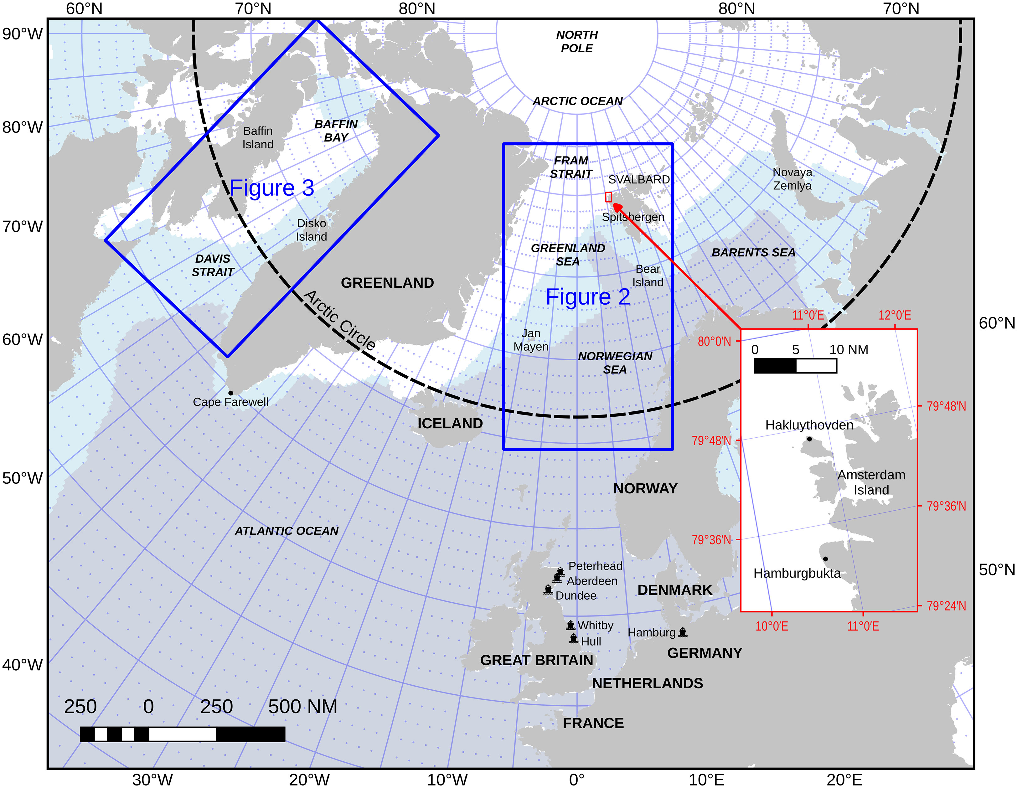
Figure 1 Map showing the Arctic whaling region of the North Atlantic Arctic, with the principal uropean nations involved in the trade as well as key localities. It also displays the typical 19th century sea ice cover during winter (March: light-blue shading) and summer (August: white shading) for the 1850s from Walsh et al (2017) Red box shows the north-eastern reaches of Svalbard where shore-based whaling occurred, blue box (left) indicates the Greenland Sea whaling grounds covered by Figure 2 and the blue box (right) denotes the Davis Strait whaling grounds covered by Figure 3. Note: Bowheads taken from the Greenland Sea are from the East Greenland-Svalbard-Barents Sea stock and those in the Davis Strait/Baffin Bay area are from the East Canada-West Greenland stock (Baird and Bickham, 2021).
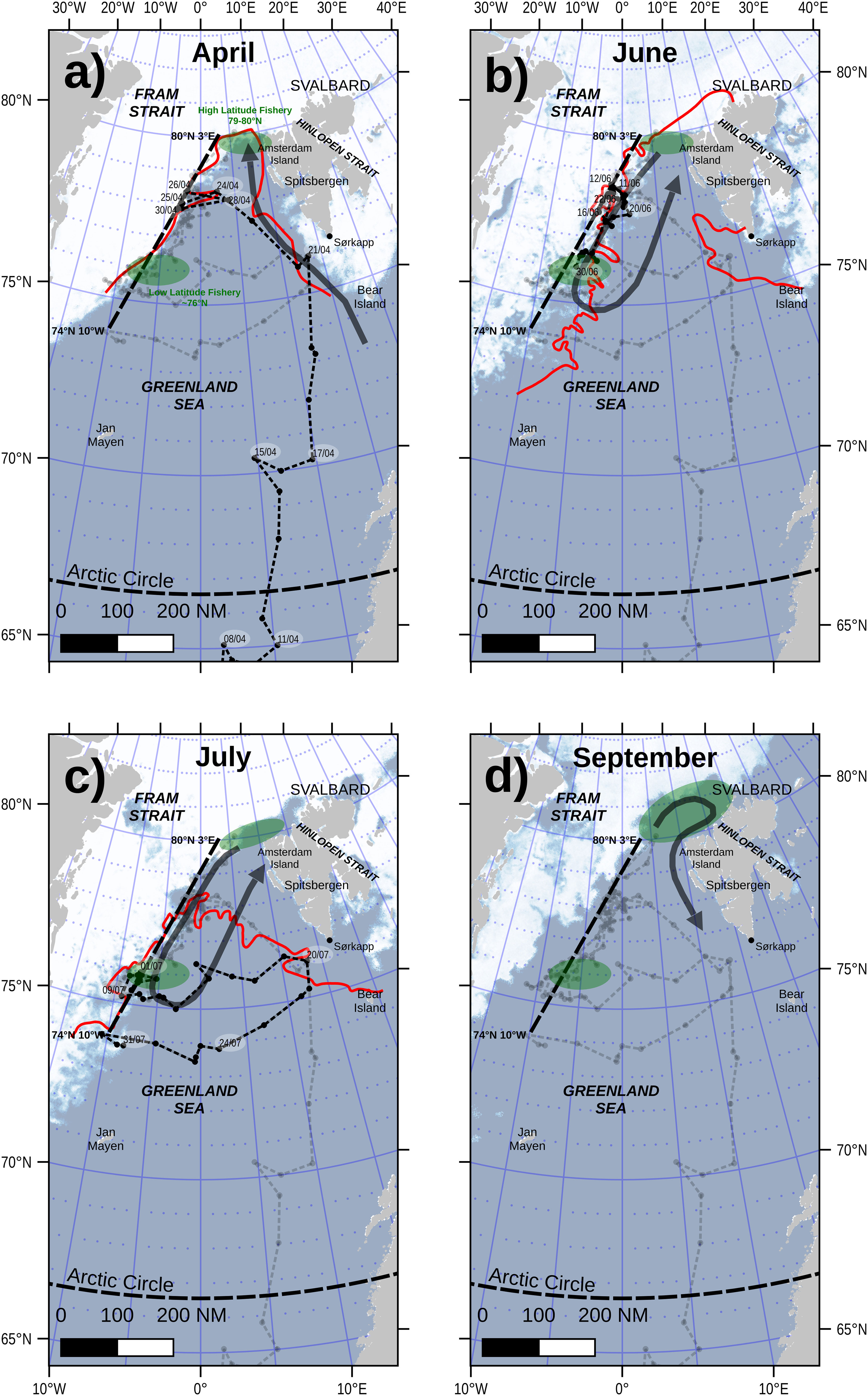
Figure 2 Map showing the whaling regions of the Greenland Sea for the months (A) April, (B) June, (C) July, and (D) September. High and low latitude whaling grounds (green ellipse). Underling ice cover (shading: white) is present satellite observations at the end of each month. Historic ice edge (Red line: from ACSYS, 2003). General monthly route of whaling ships hunting the East Greenland-Svalbard-Barents Sea stock (black arrow). Ship route of 1817 the Esk (Scoresby, 1820) where the black line for active month, otherwise grey shaded line. Generally, the most productive fishing grounds were to the west of the black dashed line. Bowheads taken from the Greenland Sea are from the East Greenland-Svalbard-Barents Sea stock (Baird and Bickham, 2021).
The explicit purpose of this manuscript is to extend previous work on North Atlantic bowhead populations (Ross, 1979; Mitchell and Reeves, 1981; Ross and MacIver, 1982; Allen & Keay, 2006; George and Thewissen, 2021b) by re-examining the British whaling records, especially records of the numbers of whales caught, the length of longest whalebone (baleen) and amount of oil yielded. By doing so we hope to quantify better the length of the whales caught, to determine whether there was a size differentiation between bowhead whales within the Greenland (EG-S-B stock) and Davis Strait (EC-WG stock) whaling grounds (Figure 1), and if this size distribution remained consistent over time. This is important as changes in the length of whales could indicate a shift in their ecology. Furthermore, as size is generally correlated with age and hence with sexual maturity (Cosens and Blouw, 2003), it could also reflect hunting pressure as whales of a certain size are removed from the gene pool.
This manuscript describes the history of whaling in the European Arctic, before analysing data from the newly produced British Antarctic Survey’s Arctic Whaling Database (BAS-AWD). This includes a discussion on the number of whales killed by the industry, with the quantity of oil and blubber secured from each voyage. After this, we refine the algorithms that enable the length of the whales caught to be estimated from the volume of oil produced or the length of their longest whalebone. The British fleet exploited both the Greenland grounds (Figure 1) and Davis Strait grounds (Figure 3), so data from these whaling regions are treated separately to allow comparative analyses between the stocks.
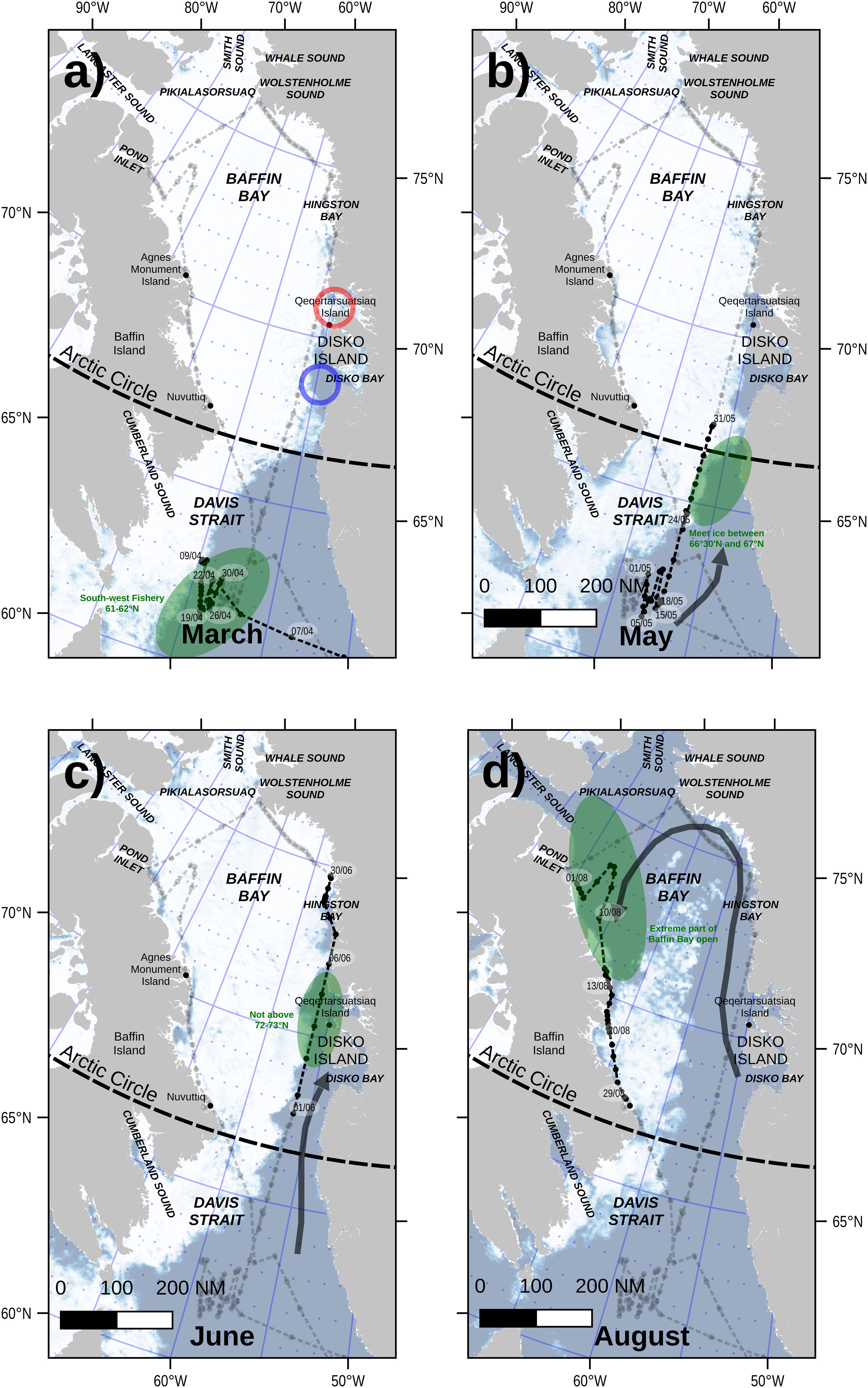
Figure 3 Map showing the whaling regions of the Davis Strait for the months (A) March, (B) May, (C) June, and (D) August. Active whaling grounds for month (green ellipse). Underling ice cover (shading: white) is present satellite observations at the end of each month. General monthly route of whaling ships hunting the East Canada-West Greenland stock (black arrow). Ship route of 1831 Dordon (black dotted line for active month, otherwise grey shaded line; Ayre, 2014). South East Bay (red circle) and North East Bay (blue circle) also identified. Bowheads taken from the in the Davis Strait whaling grounds area are from the East Canada-West Greenland stock (Baird and Bickham, 2021).
Historical setting and context
Commercial Arctic whaling started in 1611 within the fjords along the west coast of Svalbard (Figure 1: red box). This was because each summer the bowhead whales (EG-S-B stock) congregated in large numbers in these fjords, and were easy to approach. As such, whaling was very much a land-based activity, with the men living in tents and huts ashore. This period was known as ‘the Shore Fishery’ (Jansen, 1864). The English, Dutch, French, and Danes each had their preferred fjords, where whales were hunted, the oil was extracted from blubber, and the whalebone was cleaned. The English established their camps in the several bays within fjords along the coast of western Spitsbergen, while the Dutch, French, and Danes established theirs on Amsterdam Island [Amsterdanøya] in northwest Spitsbergen. Whalers from what is now Germany arrived in 1642 and settled at Hamburger Bay [Hamburgbukta], just beyond the Dutch limits (Conway, 1906, p187). A shore fishery was also established on Jan Mayen (71.0° N, 8.3° W) in 1615 by the Dutch (Barr, 1990). At first it was extremely successful, as on many occasions the catch was so good that the storage was insufficient (Muller, 1874 p151). However, in 1632 ice surrounded the island for an extended period preventing ship access, and in 1634 the Dutch seemed to have abandoned the island (Muller, 1874 p151; Holland, 1994). Whether their abandonment was due to climate, lack of whales, or whaler-on-whaler conflict is not clear (Degroot, 2022).
As commercial whaling developed, the whalers improved their knowledge of the movement of the ice, the currents, the weather around Spitsbergen, and more importantly whale behaviour. For example, Van der Brugge (1634) who wintered on Svalbard in 1633-34, reported that the whales left the fjords in late October and returned in late April. With this knowledge, the whalers timed their journeys to coincide with the periods when the fjords would be ice-free, and the whales present. This meant that they sailed for Svalbard in early spring arriving in late May, to early June, and returning home in the middle to late August (Jansen, 1864). Upon their return to their port the whale oil and whalebone processed on the beaches of Svalbard were sold.
Despite the tremendous number of whales that were killed in the initial decades after shore-based hunting began (1611), the whales continued to aggregate during the summer in their favoured fjords in large schools of 200-300 animals, which consisted of families of two to four generations (Conway, 1906, p196; Jenkins, 1921, p144). However, after about 30 years of shore-based whaling the whales no longer frequented the fjords in such great numbers (Jansen, 1864). As soon as the scarcity of whales was noticed by the shore fishery, the Dutch whaling company directors made great efforts to explore further afield. The whalers had seen the whales fleeing the fjords by either swimming to the west towards Fram Strait, or to the north-east along the north coast of Spitsbergen. By following them, two additional whaling grounds were found. The first, known as the ‘To-the-Eastward’ were located along the north-eastern shores of the Svalbard archipelago, in and beyond Hinlopen Strait. The grounds to the west were within the drifting ice between Greenland and Spitsbergen, which was called the West-Ice whaling grounds and would later be known as the Greenland Sea whaling grounds. Interestingly, Jansen (1864), p 168) mentions that the whales that took flight to the West-Ice, were different from those that swam To-the-Eastward whaling grounds, but gives no other details.
Move to pelagic whaling
By 1640-50 the bowhead whales no longer ventured into the fjords of Svalbard, thus the whalers had to adapt techniques to catch whales amongst the drifting pack of the West-Ice. Elking and Eyles (1722) mentions that the whales could be found only within the drift ice, and those ships that would not venture far into the ice often returned without catching a single whale. This shift towards whaling within the West-Ice represented a significant change to the method of whaling. It meant the shore-based structures, such as warehouses, cookeries, etc, were of no use, as the whales must be flensed at sea (remove the blubber from the body, the remaining carcass known as the krang) with the blubber and whalebone stowed on board. These products were carried to their home ports for further processing and refinement. Unfortunately, exact details on the number of ships that participated in the shore-based whaling from each county, the number of whales caught, the amount of blubber/oil obtained and other catch details. are particularly scarce. A significant effort is still needed to examine historical records to understand the extent of the shore-based whaling by each country involved.
The transition to pelagic whaling amongst the West-Ice came easier for the Dutch as they had gained the ‘in ice’ experience by sailing amongst the ice floes during their exploration of whaling grounds within the fjords of Spitsbergen. By 1640 some Dutch ships in 1640 successfully worked in the open sea beyond the fjords (Conway, 1906). As early as 1642 there were reports of blubber being brought to Holland for processing, which suggests that pelagic whaling was established by this time.
The Dutch domination was to last almost a century, with the British not returning to the trade until 1724 when an Act of Parliament designed to reinvigorate the trade promised to pay 3 shillings (15 pence) per pound (lb) of whalebone, oil or blubber caught in the Greenland fishery. It was not until 1733 that British Arctic whaling first began to recover, the then current Prime Minister Robert Warpole realised that acts of previous parliaments had failed to reinvigorate the trade and introduced a bounty of 20 shillings (one pound) per ton of displacement to ships of 200-400 tons. This did little to motivate the British fleet, and it was only after its second increase in 1749 to 40 shillings per ton, that the bounty had the desired effect of stimulating the British whaling effort (Jenkins, 1921).
Greenland Sea fishery and the EG-S-B stock
With the continued decline in the number of EG-S-B stock frequenting the coastal fjords of Svalbard the Dutch, French and Germans began hunting them within the drifting ice in earnest in the 1650s. The Dutch had already established a near-monopoly over the European whale oil market, but interestingly, the English continued to operate their land-based whaling stations. By clinging to the fjords long after whaling there had ceased to be profitable (Jenkins, 1921), the English did not learn the craft of pelagic whaling within the drifting ice (Conway, 1906 p 200). This caused the English whaling endeavour to stagnate and practically collapse by 1650.
To hunt the whales within the sea ice, away from the coast, required vessels that could withstand ice pressure, but even with such ships the risks of pelagic whaling were greater than shore-based whaling, and each year vessels and men were lost. Whaling in the waters north of 78°N was known as ‘northward-fishing or the northern whaling grounds’, and whaling at lower latitudes was called ‘southward-fishing or the southern whaling grounds’.
Scoresby (1820) suggested that the most productive whaling grounds were in the northern whaling grounds between 78° to 80°N, and that at least 90% of the whales seen in a season occurred, with some interruptions, between 80°N, 2° to 3°E to the latitude of 74°N 5° to 10°W (black dotted line in Figure 2). Scoresby (1820) adds that the whales were usually found in most abundance at the ice edge, near Hakluyt’s Headland [Hakluythovden] (Northeast Spitsbergen), in the latitude of 80°N.
Manby (1823) comments that prior to the early 19th century whaling vessels hunted predominately in the northern whaling grounds, about the latitude of 78°N, and never exceeded the longitude of 2° west. However, after 1814, whales in the northern whaling grounds became scarce, and the British whalers began to explore the seas farther to the southward (southern whaling grounds), but without proceeding far into the ice, or remaining among it beyond the middle or end of July. The prevailing idea was that it was not only useless, but extremely dangerous, to be within in the ice after this (Scoresby, 1823).
Jansen (1864), p169 describes the Dutch whaling strategy as follows. The whalers would first sail to the northern whaling grounds off the west coast of Spitsbergen, and at around 79-79.5°N. They would turn west and enter the West-Ice (see Figure 2A) and after a while would drift with the ice field into the southern whaling grounds, to around 75°N searching for whales (see Figures 2B, C). Scoresby (1820), p 208-210) agrees with the Dutch strategy of whaling and adds the whalers focused their efforts on these northern whaling grounds, but does mention that between April and July whales were sometimes caught at latitudes around 76°N (in the southern whaling grounds). However, these more southern locations were unsheltered and constantly exposed to severe swells, thus they were not popular with the whalers.
As they sailed, they observed the colour of the surface waters. Scoresby (1820) p336) noted that if the waters were transparent, blue, or greenish-blue, no whales would be found, however when they were cloudy, or of a deep olive-green colour, the whales would congregate. It is now known that the cloudy or olive-green waters Scoresby was referring to were the results of spring primary production bloom that is initiated by break up of sea ice (Carmack & Wassmann, 2006). Scoresby (1820) also noted that when a ship approached a substantial field of ice with whales swimming within it, it was usual for the ship to moor to the leeside of an adjacent ice field. Boats were lowered and placed on watch on each side of the ship at stations of about 100 to 150 yards (91 – 137 m) from each other along the ice edge. It was common for a great number of ships to moor to the same ice floe. Scoresby comments that at the Greenland whaling grounds over 100 Dutch ships might be moored to the same field of ice, with each having two or more boats on watch. As a result, the ice field would be surrounded by boats ensuring that it was almost impossible for a whale to surface for beathing near the ice edge without being within the reach of a harpoon.
Once a ship had obtained a full cargo of blubber it sailed for its homeport. However, if a full cargo had not been obtained by the time 75°N had been reached during the southward drift, it sailed back again to 79°N, or thereabouts, to make the same circuit again (arrow in Figures 2B, C). In some instances, whalers, if few or no whales were caught, would prefer to sail to the old whaling-grounds ‘To-the-Eastward’, near the east coast of Svalbard or to Novaya Zemlya.
In unusual years, when the ice east of Novaya Zemlya drifted in greater quantity to lower latitudes than in a normal year i.e., much to the south of Bear Island [Bjørnøya], there was a great abundance of whales, this was called a South-ice-year and the whale known as a South-ice whale (Jansen, 1864, p167). During these rare South-ice-years the whalers did not go to such high latitudes, but instead steered east to work as soon they detected that it was such a year. This description of a South-ice year bears a close resemblance to the conditions British pelagic whalers would later term a Close-season. A Close-season was when an extended barrier of sea ice extended from Jan Mayen in the west to Bear Island (Bjørnøya) in the east, thus preventing ships from sailing northwards to Spitsbergen. During these years the whales could be found in great abundance in this more southerly region. Muller (1874), p167) talks about the Dutch establishing camps on Spitsbergen’s east coast, to take advantage of a South-ice-year, but gives few details. Scoresby (1820), p208) also mentions that in rare instances whales were seen on the edge of the ice extending from Bjørnøya to Point Look-out (Sørkapp, the southerly point of Spitsbergen), in the early part of the season.
These historical descriptions of where the whalers hunted the EG-S-B stock fit well with contemporary movements of this stock (Lydersen et al., 2012; Kovacs et al., 2020).
About a century after Arctic commercial exploitation of the EG-S-B stock had commenced in the seas around Svalbard, the Dutch, Danish and Germans whalers extended their operations to the west coast of Greenland. These whaling grounds, where they exploited the EC-WG stock, were known as the Davis Strait fishery.
Davis Strait fishery and the EC-WG stock
In 1616, William Baffin described the large number of whales (EC-WG stock) frequenting the Davis Strait region, and how easy it was to strike a whale as they were unaccustomed to being chased. In a letter to Sir John Wolstenholme regarding his voyage he mentions that whales were ubiquitous and found in Whale Sound, Smith Sound, Wolstenholme Sound, among other regions. He proposed that whalers should visit the region the following year, however, it was not until 1719 that the first data from the Davis Strait whaling grounds were reported by Dutch writers. However, Ross (1979) points out that before 1719 there was a century of irregular whaling trade along the west coast of Greenland by vessels from Holland and Denmark. Whaling data of many of these earlier voyages are presently lacking. The first record of British ships whaling in Davis Strait were three of the South Sea Company’s fleet that went to the region in 1727.
British ships intended for the Davis Strait grounds commonly left their home port slightly earlier than those intended for Greenland grounds, sailing from late February to mid-March (Scoresby, 1820, p382). The ships first worked the South-West fishery, located along the northern part of the coast of Labrador, and near the outlet of Hudson Strait (between 61°N and 62°N) and by mid-March were generally near Cumberland Strait (Eschricht et al., 1866 p15). It was a particularly dangerous fishery due to the combination of long nights, exposure to storms, and frequency of swells. The flensing of a whale in the South-West was more hazardous than elsewhere due to the prevalence of persistent swell (Scoresby, 1820 p389). Those who persevered in the South-West, usually remained at this fishery until the end of April or the beginning of May (Figure 3A). They then navigated to the north-east along the ice edge, eventually entering the open-water that forms in late spring along the south-west coast of Greenland.
There were a few sea ice ‘choke points’ that could prevent the whalers from progressing northwards along the Greenland Coast. At the latitudes between 66.5°N and 67°N the ice was often connected with the west coast of Greenland, (Figure 3B). Once through this barrier there was another considerable barrier of ice at 68°N, immediately beyond and about 10 to 20 km from land, the whaling was reported to be good. As the summer advanced the ice continued to open, allowing ships to progress to waters around Disko Island in early May. The main fishery was on the south side of Disko Island. Generally, by the end of May or the beginning of June ships could pass a further barrier of ice lying about Hare Island [Qeqertarsuatsiaq] (70.4°N, -54.9°W)),; Figure 3C. Here they worked the northern inlets, bays and fjords frequented by the whales, particularly South East Bay, and Jacob Bight (also known as North-East Bay), (Lubbock, 1937, p208).
During June the ships would still be below 72°N or 73°N, because ice was still closely packed at those latitudes up to the coast. Whaling was largely restricted to this region around Disko Island until 1817, when Scottish Masters Muirhead (Leith) and Valentine (Aberdeen) navigated the leads between the landfast ice and main pack (known as the middle ice) and into the open water of Pikialasorsuaq or the north water polynya (Figure 3D) (Sanger, 2016). The next year Ross and Parry, explored this route and encouraged by the presence of His Majesty’s Naval Ships the majority of the whaling fleet followed. By doing so they discovered great numbers of whales in the northern regions of Baffin Bay, as well as along the eastern side of Baffin Island.
Generally, British whalers arrived in the neighbourhood of Lancaster Sound and Pond’s Bay [Mittimatalik/Pond Inlet] around the commencement of July (Young, 1867). To arrive at this date, it was necessary to follow the indentations of the Greenland coast, pushing forward whenever the pack is driven out to sea by the wind; but when the wind drives the pack towards the land the ship is to hold to the ice still attached to the shore, and even at times cut a dock with large ice-saws to protect the ship against the drifting ice (Young, 1867). This seasonal circumnavigation of Baffin Bay became the de facto voyage route for most of whalers plying the Davis Strait grounds post-1817 (Lubbock, 1937; Sanger, 2016).
As whales became scarce over time, and steam-powered ships became the norm (after 1850), whalers tended to stay longer, working their way up and down the east coast of Baffin Island until the return of winter forced them south. In the final decades of the trade, during the latter half of the 19th and early 20th centuries, the lack of bowheads led to the diversification of the trade and the establishment of wintering shore stations, to take advantage of autumn and spring whaling that was inaccessible to ships (Sanger, 2016). The historical descriptions of where the whalers hunted the EC-WG stock also fit well with contemporary movements of bowheads in the region (Heide-Jørgensen et al, 2021).
Historical catches
England re-entered the pelagic Arctic whaling industry in 1725 and Scotland a few years later in 1727. Both countries, along with other European countries, continued to send ships to the Greenland Sea and Davis Strait whaling grounds for some time, however by the latter half of the 19th century most European countries had left the industry leaving the British to hunt the remaining bowhead whales. To put the British whaling effort (from the BAS-AWD) into context with the main European whaling countries, Holland and Germany, sailings and whale catches for all three nations are shown in Figure 4. Annual whaling statistics for the Dutch have been published by De Jong (1983), for the years 1661 to 1826 using sources such as Watjen (1919) and Zorgdrager (1720). De Jong also published statistics for the major whaling port of Hamburg for the years 1669 to 1801, which were obtained from Grübe (1846)
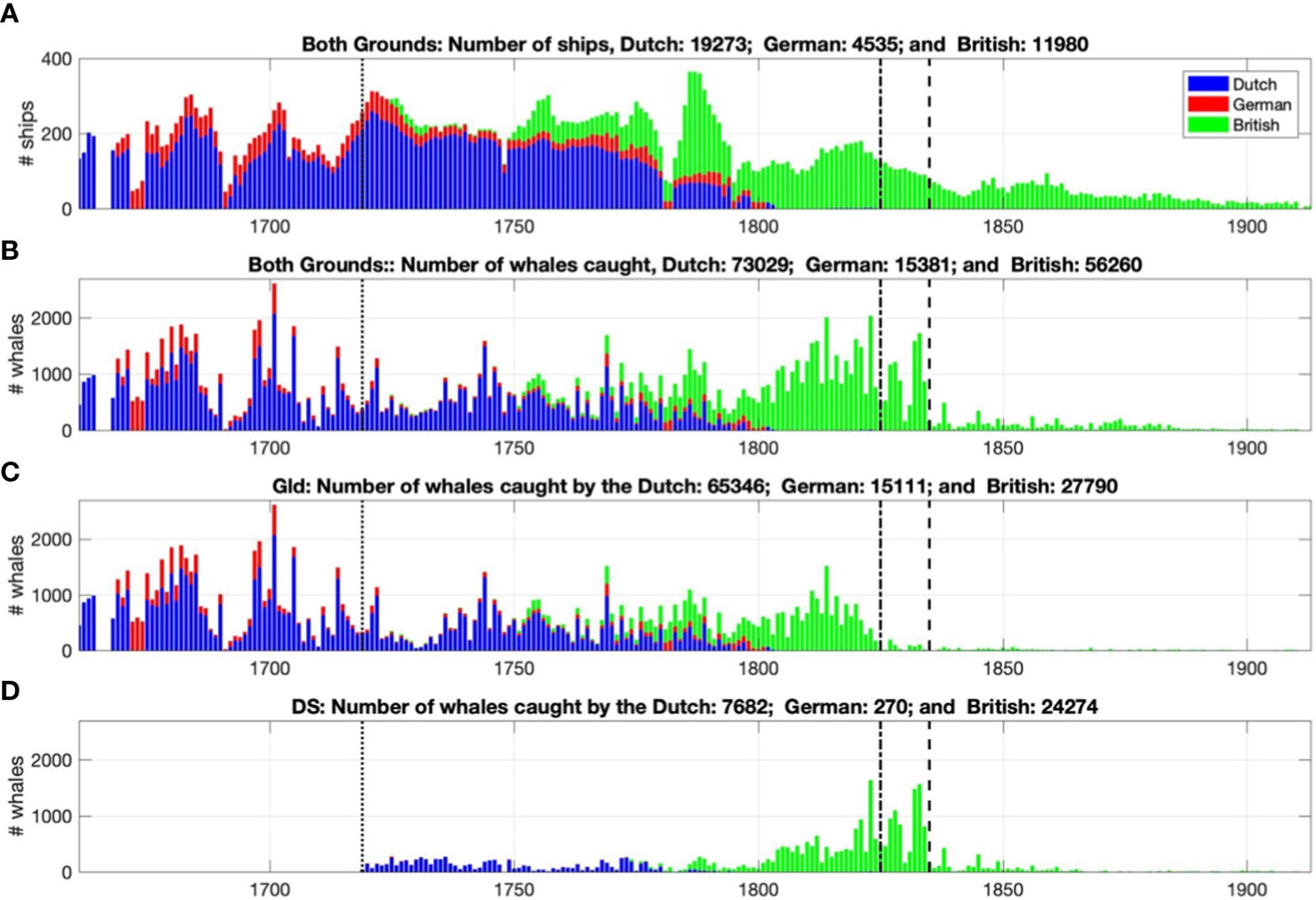
Figure 4 (A) Number of ships involved in Arctic whaling from Holland (blue), Germany (red) and Britain (green). (B) Number of whales caught from the Greenland grounds (Gld): East Greenland-Svalbard-Barents Sea stock, and Davis Strait (DS) whaling grounds: East Canada-West Greenland stock. (C) Number of whales caught from the Gld whaling grounds. (D) Number of whales caught from the DS whaling grounds. Black dotted line represents the start of whaling records within DS; the black dot-dash line represent the collapse of the East Greenland-Svalbard-Barents Sea stock; and black dashed line represent the collapse of the East Canada-West Greenland stock. As the whaling location of some vessels are not known, or they whaled in both Gld and DS the whales they caught are not included in the numbers for Gld (plot (C)) or DS (plot (D)) respectively.
Figure 4 reveals that the Dutch dominated the industry to the mid-18th century, after which the British dominated. Between 1661 and 1913 over 140,000 whales were recorded as being caught in the Greenland Sea and Davis Strait grounds. As the bowheads in the two whaling grounds are from different stocks, we have separated them into Greenland Sea (EG-S-B) and Davis Strait (EC-WG) respectively. There were over 108, 000 whales removed from the EG-S-B stock in the Greenland Sea grounds and over 32,000 from the EC-WG stock in the Davis Strait grounds. Even though this number is high, it surely represents a substantial underestimate, as it does not include data from other European whaling countries or the United States, and the German states data only covers Hamburg. The British data has many instances where the number of whales taken by a ship is presently unknown and thus uncounted. The data shown does not include whaling by Indigenous whalers, or whales and calves that were struck and lost, and may have consequently died later. It does not include any shore-based whaling data in the early years of the trade.
Material and methods
The strategic importance for a nation to be self-sufficient in whale oil and whalebone led the British (1733-1824), to introduce a bounty for a time to encourage and subsidise national efforts. To receive the British bounty, it was mandatory for ships to meet a set of requirements, one of which was the presentation of a logbook detailing their voyage and catch to the Customs Office upon their return from the Arctic (Stonehouse, 2007; Brown et al., 2008; Molloy et al., 2019). These Customs Office records, with newspaper articles, logbooks and other historical texts are the principal sources of information on the British Arctic whaling industry. The BAS-AWD has at present over 11,000 individual records of British whaling voyages to the Greenland Sea and the Davis Strait between 1725 and 1913. Where practical the data analysis has endeavoured to be comprehensive, and as a result the records contain information on the following categories: name and rig of the ship, its classification (condition of hull and rigging), its tonnage, its draft, the port and year the ship was built, its home port, its owner, name of the master, whaling grounds worked, the date of sailing and return, number of bowhead whales, bottlenose whales, narwhals, beluga whales, seals, walrus, and polar bears caught, as well as the weight of whalebone (baleen) taken, the amount of whale oil and blubber and the amount of seal oil and blubber produced. However, the record-keeping is incomplete as a result not all information within these categories is available for each voyage. In this manuscript, we only report on data related to bowhead whales.
To compile the BAS-AWD, we collated and cross-checked data from numerous sources, the prominent ones are listed in Table 1. The BAS-AWD enables the interpretation of aspects of the British Arctic whaling trade in finer detail than was previously possible. The analysis of the BAS-AWD was performed in MATLAB, and in many cases we use normalised histograms to display the data. With this normalisation, the height of each bar is equal to the probability of selecting an observation within that bin interval, and the height of all of the bars sums to 100%.
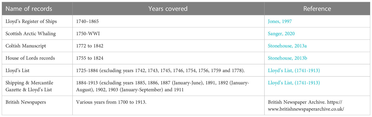
Table 1 A list of the main records that were used to compile the British Antarctic Survey’s Arctic whaling database.
To ensure only oil from bowhead whales were used in the calculations, data from ships which also captured other marine species (e.g. seals, walrus, or other species of whales) was excluded. The catching of seals became much more frequent during whaling voyages after 1841 (Brown et al., 2008; Sanger, 2016), thus our analysis is mainly limited to the period before this development. Mitchell and Reeves (1983) suggested that in the mid-1800s, some British vessels took humpback whales (Megaptera novaeangliae), and some Davis Strait whalers killed right whales (Eubalaena glacialis) (Reeves and Mitchell, 1986), so even with these precautions our approach may have some unquantifiable small errors. The procedure to (a) define the relationship between blubber and oil, (b) calculate the yield of oil per whale, and (c) calculate of the length of whales caught and are described below.
Relationship between blubber and oil
Once a whale was killed, it was towed to the side of the ship and the thick layer of blubber peeled from the carcass; a process known as flensing or flinching. The whalebone (baleen) was then removed and the remaining carcass, termed a krang was discarded. In a process termed ‘making off’ the blubber was cut down into small chunks, often using the whale’s tail as a chopping board so as not to dull the knives, and packed into wooden casks and later metal vats, which were stowed in the ship’s hold (Archibald, 2013). Final processing of the blubber and whalebone was accomplished when the ship reached its home port. Once the casks were landed the blubber was removed and placed into large copper vats where it was boiled. This separated the profitable oil from the refuse (Buchan, 1993). The term blubber is used to describe the raw material (fat, connective tissues, etc.) obtained before the boiling process, whilst oil is the fully-processed, commercial product (after boiling).
Because whale products had a relatively high commercial value each vessel in the trade should have maintained an accompanying record of the number of whales caught, the tonnage of blubber and the weight of whalebone. In addition, the British generally recorded the volume of refined oil, in some instances the length of the longest whalebone plate and on rare occasions the length of the whale itself. The volumes of blubber and oil were either measured in butts or tuns (old English units of liquid volume), with two butts equalling one tun.
Scoresby (1820) noted that a ton, or 252 gallons by volume, of blubber yields between 202 to 187 gallons of oil, with the rest being a mixture of collagen fibre and elastic fibre (protein) matrix, blood vessels and water. This suggests that the quantity of blubber (pre-boiling) to oil (post-boiling) is between 74% and 80%. In a report by John Sanders, surgeon on Samuel in 1789, he suggests that 3 tons of blubber gives 2 tons of oil (66% yield), but goes on to note that those involved in the blubber boiling say it can produce substantially more (Lubbock, 1937, p129).
There are many instances within the BAS-AWD where a ship recorded both the volume of blubber and the subsequent volume of oil it produced (n=1,059). Thus, dividing the volume of oil by the volume of blubber were able to quantify the yield of oil from the boiling process.
Calculation of the yield of oil per whale
The standard recording method for British whaling ships was for them to provide the total number of whales secured by a ship in a season with the volume of blubber and/or oil obtained and the weight of whalebone yielded. To reduce uncertainty we only utilised records where the volume of oil was registered. To calculate the yield of oil per whale for a particular ship for a particular year the number of whales caught was divided by the quantity of oil extracted. As the whaling data within the BAS-AWD are collated per vessel, and not per individual whale, these calculations should be regarded as an average estimate of yield.
As with the calculation of the blubber to oil ratio, we tried to ensure that only bowhead whale oil was utilised when calculating yield, thus any voyage where other species were captured was excluded. As the EG-S-B and EC-WG stocks are distinct we have further subdivided the analysis of the data into the bowhead whales from the Greenland Sea and those of the Davis Strait region. We excluded data where ships visited both grounds, or data where it was unclear which whaling grounds were visited. Despite the limitations placed on the data we still have 1,036 unique oil yield values for the Greenland Sea and 1,756 for Davis Strait (see Figure 5).
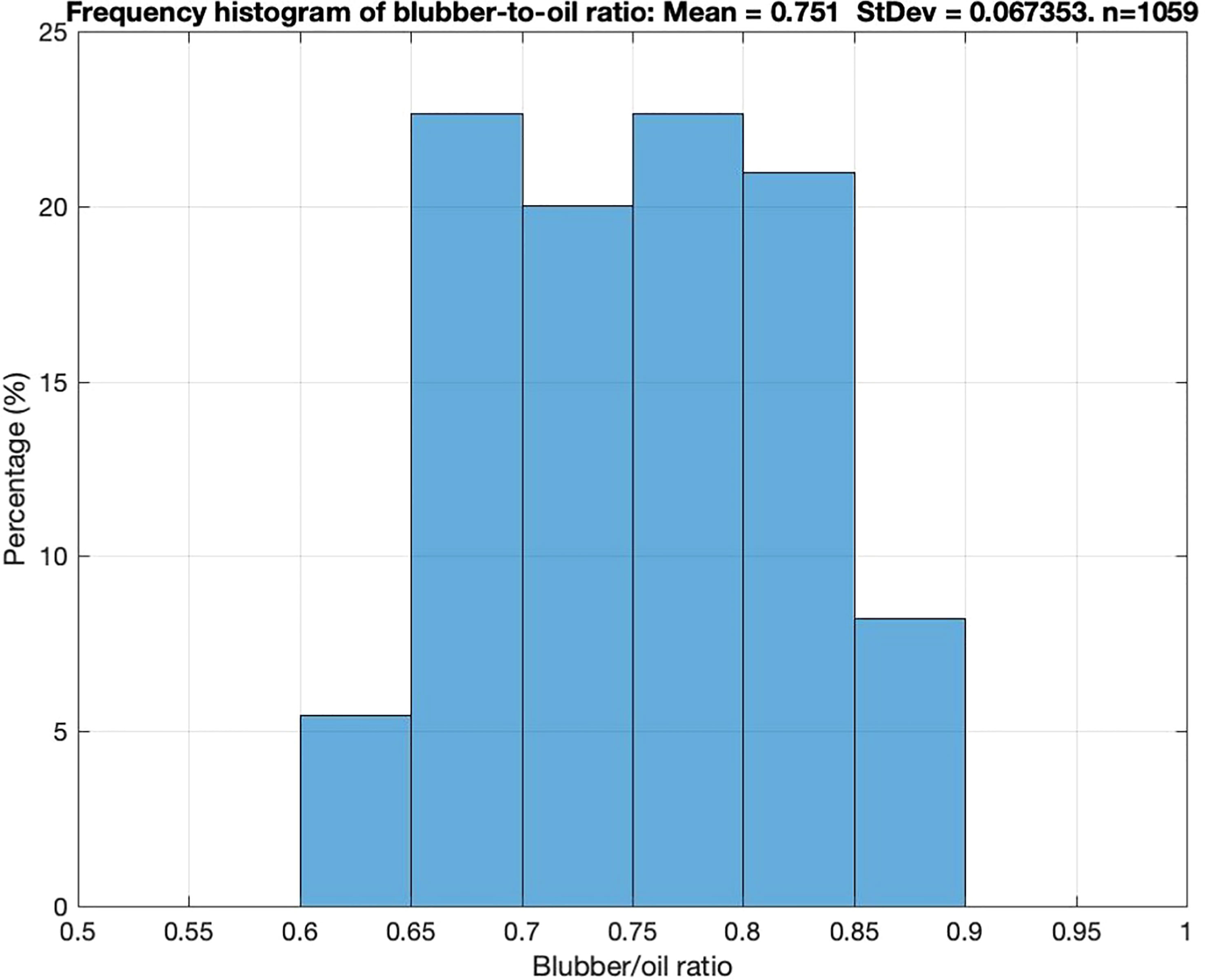
Figure 5 Plot showing the frequency histogram of the ratio of blubber to oil. Blubber to oil ratio is along the x axis (in 0.05 bins), and their respective percentage on the y axis.
Calculation of the length of whales caught
It is exceedingly difficult to envisage a whale’s dimensions when only the amount of oil extracted from it is known. The length of a whale (head to tail) is a much more tangible parameter. Unfortunately, such lengths were rarely recorded as it would have been a difficult and unnecessary process at sea. We attempt to resolve the conundrum by using the work by Scoresby (1811), Scoresby, 1820), as well as Finley and Darling (1990); Lowry (1993) and George et al. (2021a), to derive an improved relationship between oil yield and the length of the longest whalebone (baleen). We then developed further the relationship between length of the longest whalebone and the length of the bowhead whale. Finally, by combining the relationship between oil yield and the length of the longest whalebone with the relationship between longest whalebone and the length of the bowhead whale we are able to estimate the length of the whale from oil yield.
The first step in this process is to determine the relationship between oil yield and whalebone length. Scoresby (1811), writes that the whalers could estimate the quantity of oil yielded by a bowhead whale by the length of the longest whalebone. To quantify this relationship, he analysed oil yield and corresponding longest whalebone data from numerous catches and presented his findings to the Wernerian Natural History Society in 1810 (Scoresby, 1811). He later improved these initial calculations by including more observations (Scoresby, 1820). These results are reproduced in Table 2. The exact number of whales used to derive this relationship is not known, but Scoresby was involved in the capture of over 300 whales, thus we assume a number of these, with observations made by others, were made to produce this table.
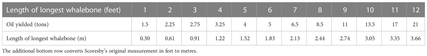
Table 2 Reproduction of the Table produced by Scoresby (1820) showing the relationship of the longest whalebone length in feet to the average amount of oil produced (in tons).
Scoresby’s table recorded whalebone in divisions of a foot which was converted to metres (1 m = 3.28 feet). Interestingly, his table displays oil yield in tons (weight) and not tuns (volume) as is standard practise. Scoresby (1820), p461) stated that an English ton of oil is equal to 1933 lbs, 12 oz 14 dr at 60°F (15.6°C), which is equivalent to 877.16 kg. Given that a ton in the avoirdupois system of weights and measures (that Scoresby used) is equivalent to 2000 lbs (907.19 kg), the conversion from 1 ton of oil to 1 tun oil is equal to 907.19 divided by 877.16 tuns; or 1 ton of oil equates to 1.03 tuns of oil. Given how close this is to 1:1 ratio it may be the reason why Scoresby states that both a ‘ton or tun of oil is 252 Gallons’. Given this statement we have assumed that Scoresby views tons or tuns as being interchangeable. As a result, we have not applied the 1.03 multiplier to Table 2, and we use ton as the descriptor.
In addition to Scoresby’s table (Table 2) we have identified additional data on the length of longest whalebone and corresponding tons of oil the whale produced from the whaling ships Arctic (1873: in Markham, 1874, p 279), Eclipse (1887:in Lubbock, 1937 p419) and North Briton (1819: in Lubbock, 1937 p214), as well as additional measurements from Scoresby (1820) p 464). It is likely however, that the additional measurements from Scoresby were also used in his relationship expressed in Table 2, but for completeness we have included them.
Finley and Darling (1990) took it further and examined the statistical relationship between the body length of a bowhead whale and the length of the longest whalebone. They did this by utilising data from the whaling ship Cumbrian (Capt. Johnson) in 1823, which was presented by Lubbock (1937), p254). We supplement their work, by adding data from Scoresby (1820, p464), as well as Eschricht et al. (1866), p74) and the Eclipse (1887: Lubbock, 1937, p419) and the Narwhal which caught and measured a whale in Davis Strait in 1859. This increased the number of measurements to n=33, but more importantly allows the possibility to extend the relationship established by Finley and Darling (1990) from a previous minimum whale length of 8.5 m to below 5 m.
Results
The frequency distribution of oil yield per whale for the Greenland Sea (EG-S-B stock) and Davis Strait (EC-WG stock) whaling grounds is displayed in Figure 6. Also displayed in Figure 6 is the difference in oil yield between these two whaling grounds. To understand if the extension of whaling to new areas of the Greenland and Davis Strait whaling grounds had consequences for the oil yield a frequency distribution of pre- and post-expansion oil yields are displayed in Figure 7. To recapitulate, for the Greenland whaling grounds this occurred in 1814 where ships started the drift southward with the ice along the east Greenland ice edge, rather than staying in the northern whaling grounds. For the Davis Strait whaling grounds it was in1817 when the ships started to circumnavigate Baffin Bay rather than whaling around Disko Island.
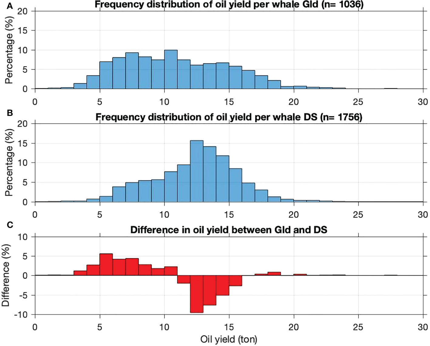
Figure 6 Normalised frequency distribution histograms showing (in 0.5-ton bins) (A) Greenland Sea (Gld) yields per whale: EG-S-B stock. (B, C) Davis Strait (DS) yields per whale: EC-WG stock, and (C) the difference in oil yield between the two whaling grounds; positive value means higher yield in the Gld.
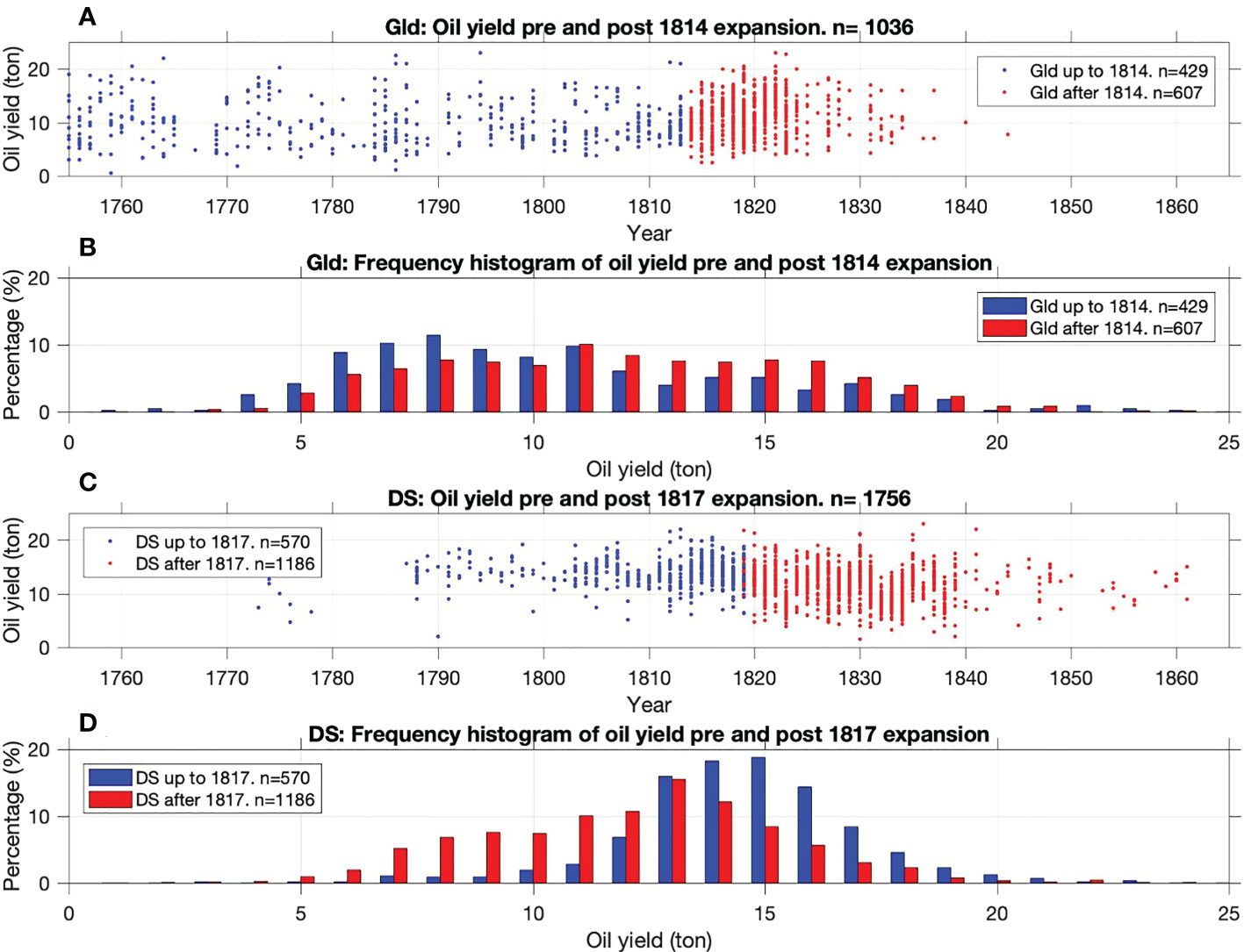
Figure 7 (A) Timeseries of oil yield from the Greenland Sea (Gld) whaling grounds, EG-S-B stock. Blue dots are pre-1814 expansion, whilst the red dots are after the 1814 expansion. (B) Frequency histogram showing in 1-ton bins the Gld oil yields pre-1814 (blue) and post-1814 (red). (C) Same as (A) but for Davis Strait (DS) whaling ground, EC-WG stock, with the pre- and post-expansion being in 1817. (D) Same as (B) but for DS oil yields pre-1817 (blue) and post-1817 (red) expansion.
Greenland Sea yields
Figure 6A displays the normalised frequency distribution of oil yield from the EG-S-B stock within Greenland Sea whaling grounds. They reveal that the oil yield per whale covers a range of values up to about 25 tons. The distribution is relatively broad and flat which suggests that British whalers in the Greenland Sea caught range of whales that yield between 5 to 15 tons of oil (average 10.7 +/- 4.1 tons of oil), with a smaller proportion of whales being outside this range. When compared to catches within the Davis Strait grounds (Figure 6C) we can see that EG-S-B stock were more likely to produce 11 tons of oil or less per whale. In contrast, the EC-WG stock (Davis Strait) were more likely to yield between 12 to 16 tons of oil per whale. In both whaling grounds only a very small percentage of the whales caught delivered less than 3 tons or more than 20 tons of oil.
Taking the 1814 extension of the Greenland Sea whaling grounds as a bifurcation point (Figure 7A) the average oil yield per whale before 1814 was 9.9 +/- 4.2 tons (n=429) and after 1814 is 11.3 +/- 3.7 tons (n=607). This difference manifested itself as a higher proportion of whales being caught pre-1814 that yielded between 4 and 10 tons and less whales that yielded between 11 and 20 tons of oil (Figure 7B).
Davis Strait yields
The Davis Strait whaling grounds also had a good spread in the yield of oil per whale, with the EC-WG stock also yielding a maximum of about 25 tons per whale (Figure 6B). However, the spread within the yield in the EC-WG stock is very different to that of the Greenland Sea EG-S-B stock. It has a more Gaussian-like distribution, centred around a yield of 12-13 tons per whale (mean 12.3 +/- 3.2 tons). There is a strong spatio-temporal element to this distribution (Figures 7C, D), with the data suggesting a higher percentage of the EC-WG stock produced larger oil yields, 14 to 20 tons, before the expansion of whaling in 1817. As mentioned, prior to 1817 the whalers used to hunt in the South-West fishery before moving to the region around Disko Island. However, after 1817 vessels sailed through the sea ice north of Disko Bay and performed an anticlockwise navigation around Baffin Bay.
Taking the 1817 extension of the Davis Strait whaling grounds as a bifurcation point, we calculate that before 1817 the average yield of oil per whale was 13.9 +/- 2.5 tons whilst after this date is was 11.4 +/- 3.1 This change can be clearly seen in the normalised frequency distribution of Figure 7D. Before 1817 a larger percentage of whales caught consistently yielded more than 13 tons, whilst after the expansion in 1817 a higher proportion consistently yielded less than 13 tons.
Length of whales caught
Our analysis shows that a third-order polynomial best describes the relationship between whalebone length and tons of oil yielded to within a few tens of centimetres at worst (see red line within Figure 8A and residual error plot in 8b). The relationship is:
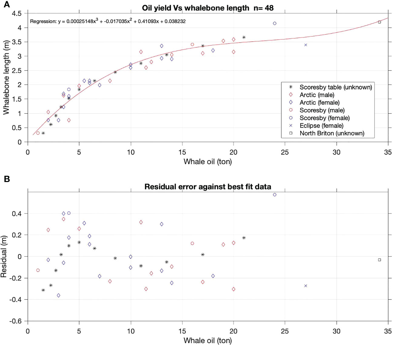
Figure 8 (A) Plot showing the relationship between the length of the longest whalebone and oil yield. The symbols represent the different data sources used to determine relationship (Eqn 1).(B): Plot showing the residual error of the difference between the data and the estimated value of calculated from the regression line. Males are in red, females in blue, and sex unknown in black.
where WBlength is the length of the longest whalebone and Woil is the tons of whale oil.
Even though the number of data points used to test oil-whalebone relationship is relatively low (n=48), they do have a good spread across a range of whalebone sizes and oil yields, although data on oil yields above 20 tons are limited. Given Scoresby’s and the Eclipse data are from bowhead whales caught in the Greenland Sea, and the Arctic, and North Briton data are from the Davis Strait, it suggests that the relationship holds for both Greenland Sea and Davis Strait whaling grounds.
Scoresby points out that there are exceptions to his rule as the volume of blubber obtained from a bowhead whale may vary depending on its size, age and nutritional state, as well as the efficiency of the crew in stripping the blubber from the carcass. Jackson (2013), p37 in his transcription of The Voyage of David Craigie to Davis Strait and Baffin Bay (1818) explains that the blubber is ‘in a variable measure of density according to the season of the year, the age, or sex of the fish, averaging in general from half a foot to one and a half or two feet; the last mentioned, is from a female that has just emitted her offspring without giving suck, turns out quite a treasure yielding twice or nearly three times as much oil as one oppositely circumstanced, or that has yielded suck for a few months.’
We can test the accuracy of Eqn 1 because Lubbock (1937), p 273 lists the whalebone lengths of 18 whales caught by the Cumbrian in 1827, but the oil yield per whale was not listed. Fortuitously, Lubbock (1937) provides the total oil yield from all 18 whales as 280 tons. Entering the whalebone sizes from Cumbrian into Eqn 1 and summing the total we get a total of 295 tons of oil, which is remarkably close to 280 tons that Cumbrian is listed as obtaining; only 5% difference. A summary is given in Table 3.
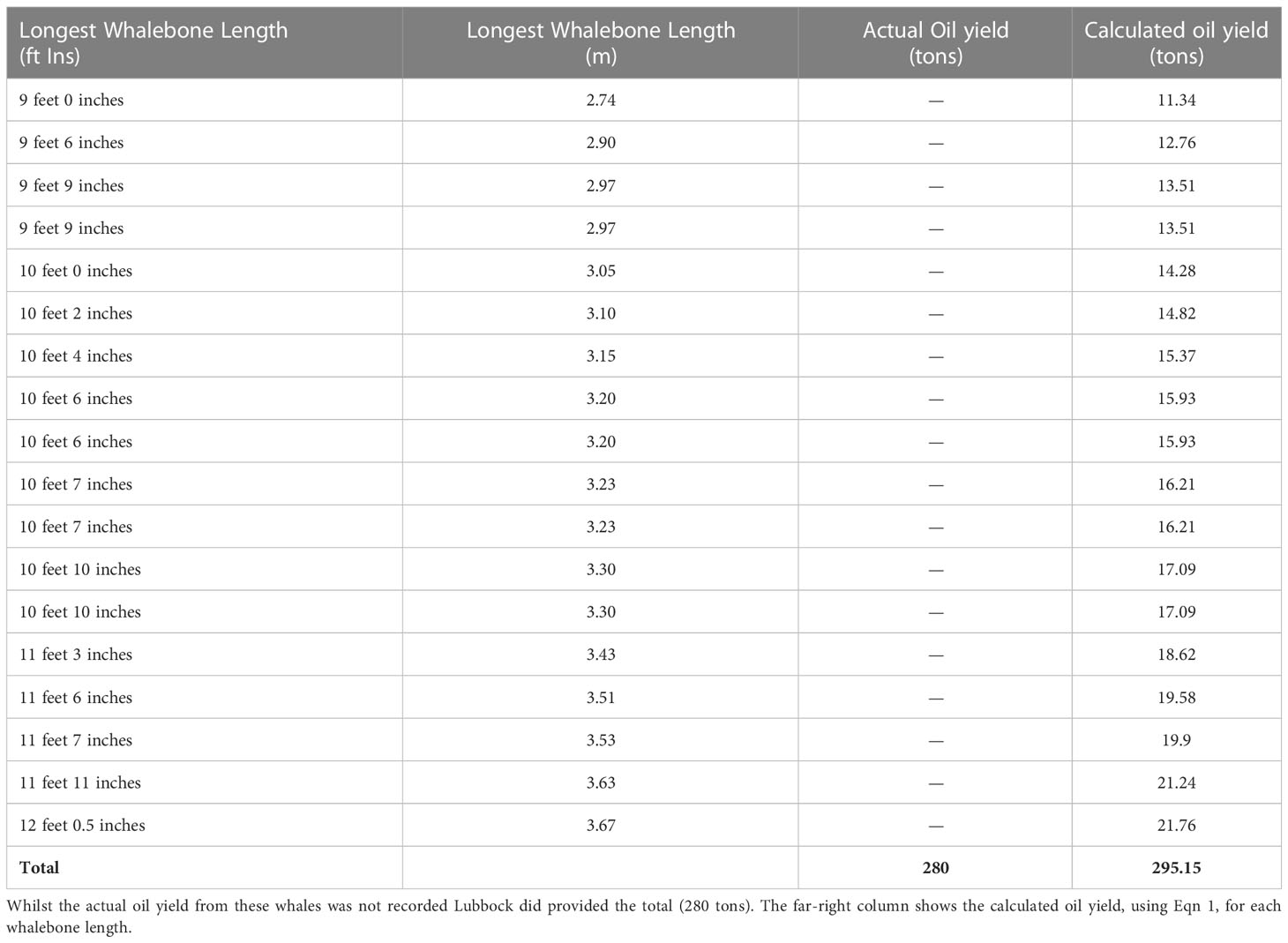
Table 3 Table from Lubbock (1937), showing the length of whalebone (in ascending length order) from the 18 whales the Cumbrian caught.
Building on tRegression analysis of the combined Cumbrian, Scoresby, Eschricht et al., Eclipse and Narwhal datasets suggests that the relationship follows:
where Wlength is total body length of the whale in metres and WBlength is the length of the longest whalebone.
The linear fit for Eqn 3 (see Figure 9A) is particularly robust as it has a R-squared value of 0.86, and a p-value which less than 0.001. The data suggest that the relationship between the oil produced and whalebone length holds for both whaling grounds as Scoresby’s and Lubbock’s data are from Greenland, whilst Cumbrian and Narwhal data are from the Davis Strait. Although not stated the Eschricht et al., data is likely to represent Davis Strait.
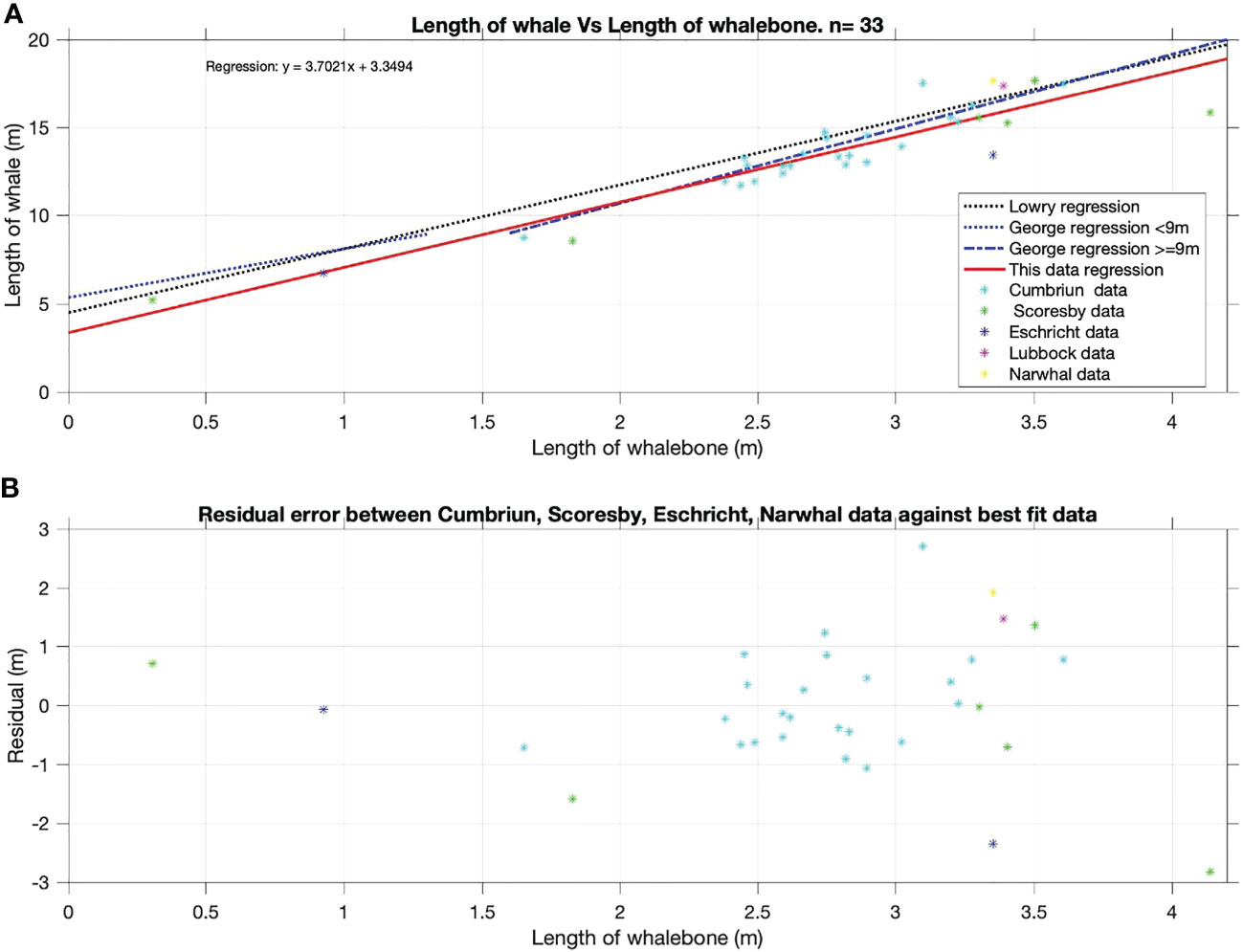
Figure 9 (A) Plot showing the relationship between largest whalebone length and the length of the corresponding whale. The symbols represent the different data sources used to determine relationship. The red dotted line represents the line of best fit for these data sources (Eqn 2), whilst the black dotted line is the line if best fit from Lowry (1993), the blue dotted line from George et al. (2021a) for whales<9 m and the blue dashed line is for George et al. (2021a) for whales >= 9 m. (B) Plot showing the residual error of the difference between the data and the estimated value of calculated from the regression line.
Combining the relationship derived between the oil yield and whalebone length (Eqn 1), with the relationship between whalebone length and the length of a whale (Eqn 2) we can derive the relationship for whale length from the oil yield. This relationship is determined as:
where Wlength is whale length in metres and Woil is whale oil in tons
The relationship can be visualised in Figure 10A, along with a very limited number of independent measurements of whale length and the tons of oil they yielded (n=7). These were from Scoresby (1820 p 464) and Eclipse (1887: Lubbock, 1937 p419) and the residual error from applying Eqn 3 to each data point is shown in Figure 10B.
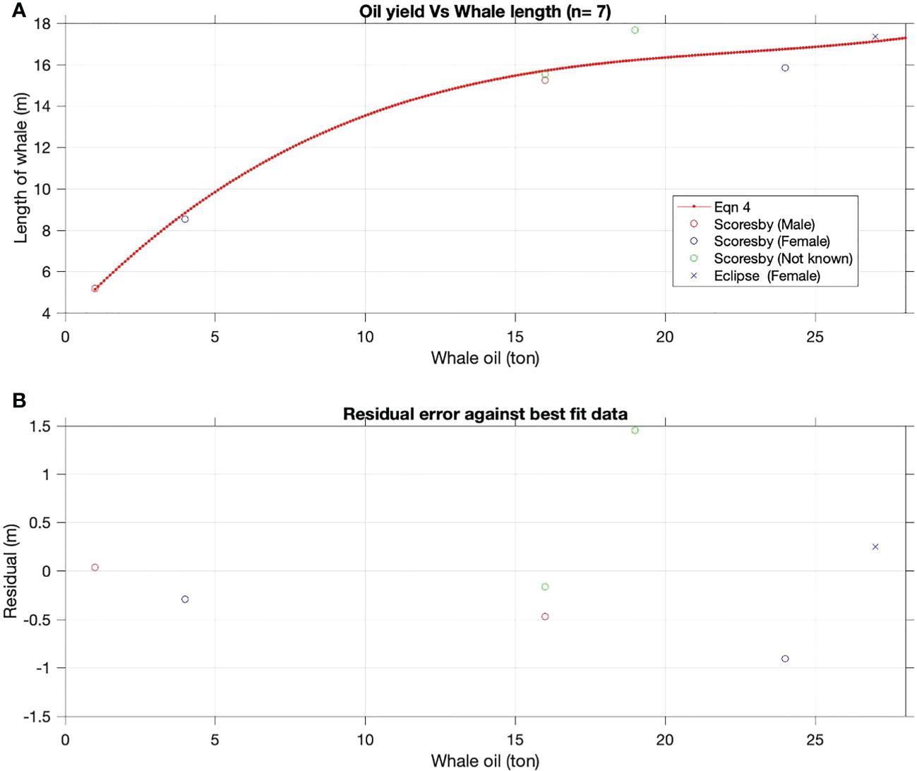
Figure 10 (A) Plot showing the relationship between the oil yield and length. The red line represents the output of Eqn 3 over different oil yield values. This was obtained by combining Eqn 1 and Eqn 2. Symbols represent the different data sources that are available to independently validate Eqn 3; Scoresby (1820) p 464) and Eclipse (1887: Lubbock, 1937 p419). (B) Plot showing the residual error of the difference between the data and the estimated value of calculated from the regression line.
Now that we have established a relationship between oil yield, whalebone length and the length of the whale we can apply this to the oil-yield data presented in Figures 6, 7. To recapitulate, this is for all records within the BAS-AWD that are from vessels that have oil yields, but caught only bowhead whales and no other species. However, it is not straightforward calculation because of the non-linearity in Eqn 3. This means we cannot use the mean yield per animal (obtained by dividing the total weight of the oil by the number of animals caught) to derive the average length of the whale. This is because the average length of a whales caught depends not only on the total amount of oil obtained but also on length heterogeneity of animals caught.
Elucidating the oil yield on a per whale caught basis is problematic because this parameter was not recorded when more than one individual was captured. Whilst we know the number of whales that were caught and their total oil yield for a particular voyage, we do not know how much oil was associated with each whale. For example, if 4 whales yielded a total of 10 tons of oil their actual allocation may have been 7, 1, 1, and 1 tons of oil respectively. To estimate the oil yield on a per whale basis we ran simulations where we randomly attributed oil yields (between 1 and 30) whose combination added up to the total known yield for the number of whales caught from a voyage. This was performed using the MATLAB function randfixedsum.m (Stafford, 2023). To ensure we have a sufficiently large spread of possible combinations of oil yields we performed these random simulation 100,000 times for each voyage. The resultant individual oil yields from the simulations were then converted to length according to Eqn 3, from which the mean length of the whales for that voyage was determined. This approach assumes there is an equal chance of catching a whale that yields between 1 and 30 tons of oil. Results are shown in Figure 11 and used in Table 4.
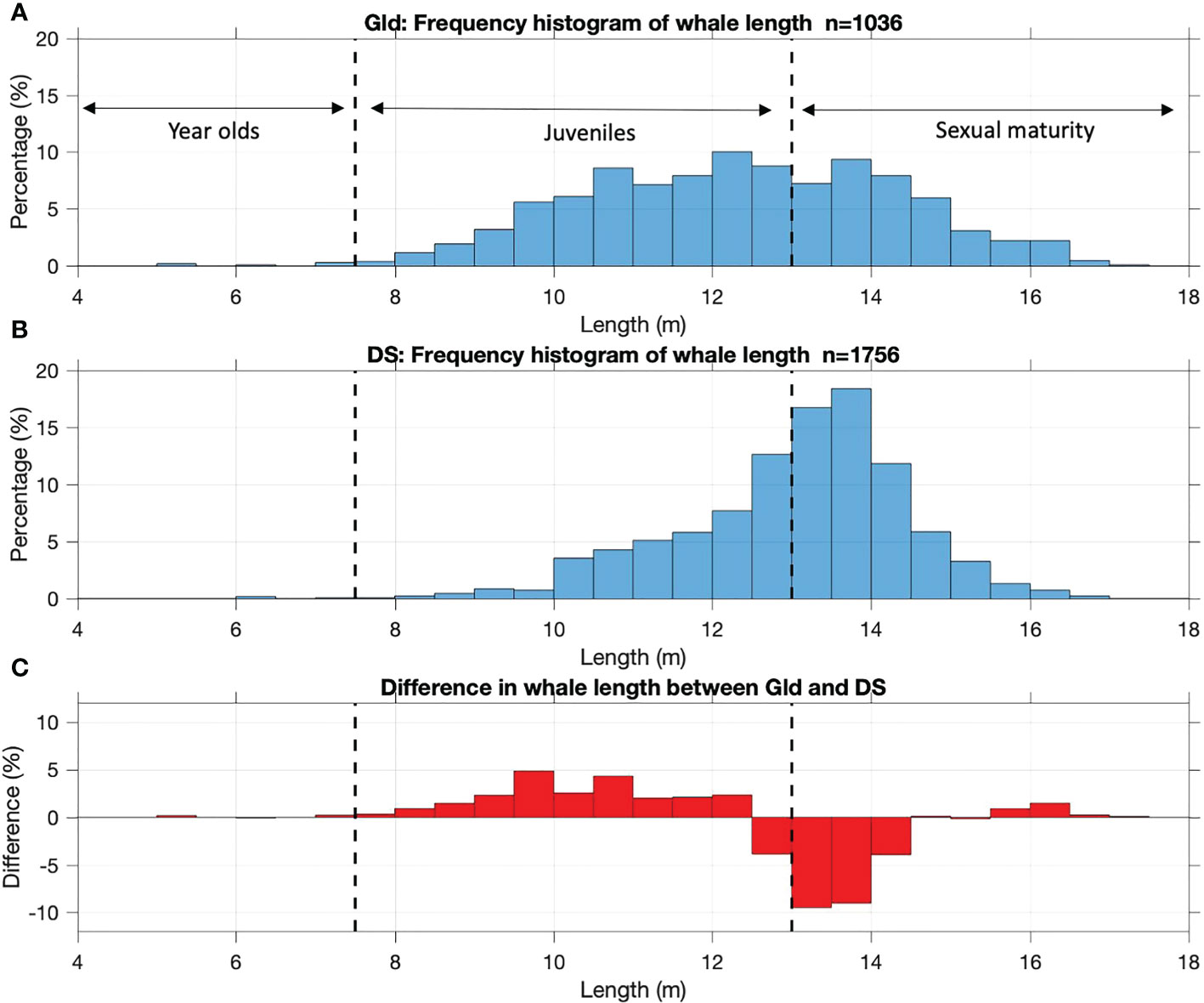
Figure 11 Normalised frequency distribution histograms showing (in 0.5 m bins) (A) whale length from Greenland whaling grounds (EG-S-B stock). (B) whale length from the Davis Strait grounds (EC-WG stock), and (C) the difference in length between the two whaling grounds; positive value means higher yield in the Greenland whaling grounds. Also included is the lengths related to maturity classes (black dotted line): (i) Year-olds: below 7.5 m, (ii) Juveniles: 7.5 m to below 13.0 m, (iii) Sexually mature: 13.0 m and above (Koski et al., 1993; Tarpley et al., 2021).
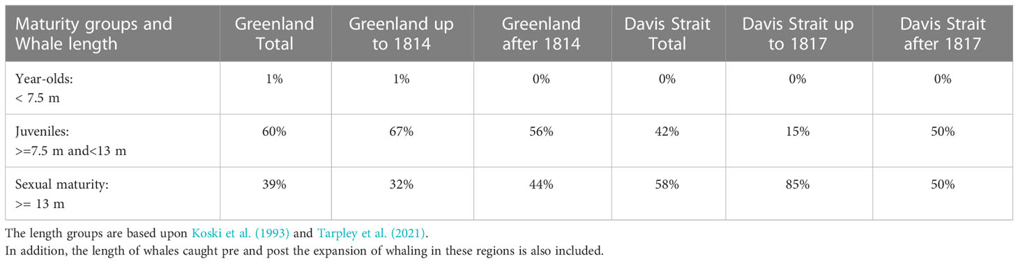
Table 4 Percentage of whales caught from Greenland and Davis Strait in the three length groups.
As with the oil yield frequency histograms (Figure 6) we see that the whale length distributions are different between the two stocks (Figures 11A, B). The EG-S-B stock shows a relatively broad and flat frequency distribution, whereas EC-WG has a much shaper Gaussian shape. Comparing the frequency distribution histogram between the two stocks (Figure 11C) we can see that there are distinct differences between the lengths of whales caught. Overall a higher proportion of the EG-S-B stock are of lengths that are less than 12.5 m, whilst significantly more whales from the EC-WG stock are between 13 and 14.5m in length. There is also a small increase in the proportion of whales caught from EG-S-B stock being around 16 m in length.
Discussion
The combination of economics and politics motivated European commercial whaling in the Arctic for several centuries, and when merged with discovery, innovation and technology it almost exhausted the EC-WG and EG-S-B stocks (Thewissen and George, 2021). It is quite remarkable that this industry was able to exploit the EC-WG and EG-S-B stocks for such a long period of time from what is essentially two relatively small regions of the world’s ocean. Our conservative estimate is that British whalers, between 1725 and 1913, removed over 56,000 whales from the region, about 28,000 from the EG-S-B stock (Greenland Sea grounds), about 25,000 from the EC-WG (Davis Strait grounds) and around 3,000 from ships that caught whales from both grounds or where their whaling location is not clearly stated. These figures can be set against the numbers caught by other European whaling countries. From Figure 4 we find that between 1661 and 1826 the Dutch removed 65,346 whales from the EG-S-B stock and 7,682 from the EC-WG, whilst the Hamburg fleet between 1669 and 1801 removed 15,111 whales from the EG-S-B stock, and 270 from the EC-WG.
The yearly harvest was not sustainable as reflected in the rapid decline in catch numbers in the Greenland Sea whaling grounds (Figure 4C) and Davis Strait (Figure 4D) whaling grounds declined to low numbers in the early to mid-19th century. This sudden decline was most dramatic in the EC-WG stock (Davis Strait grounds) which went from over a thousand animals being caught per year to just a few hundred (or less) over a couple of years. The EC-WG stock collapsed around the mid-1830s, whilst the EG-S-B stock, which were hunted in the Greenland Sea grounds, collapsed a decade earlier around the mid-1820s. The rapid collapse in the number of bowheads being caught suggests that each stock went through hyperstability phase; when catch rates remain high even as the population was being rapidly depleted. After the collapse in both stocks there were still around 70 years of unregulated whaling, making any recovery of either stock exceedingly delayed. Presently, the EG-S-B stocks number in the low hundreds (Vacquié-Garcia et al, 2017), whilst the EC-WG stocks are estimated to be around 6,500 (Doniol-Valcroze et al., 2020).
By collating the relevant historical measurements, we have been able to determine robust relationships between the length of the longest whalebone and the tons of whale oil obtained (Eqn 1) as well as the relationship between the total body length and the length of the longest whalebone (Eqn 2). This allowed us to directly estimate the length of a whale from its oil yield (Eqn 3). We have attempted to derive these relationships based on historical measurements and where possible independently validate these (e.g. Table 3 and Figure 10) or associate them with comparable measurements from other stocks (Figure 9).
The question of how these data fits with other stocks on bowhead whales, especially the Bering-Chukchi-Beaufort is a valid one as there are comparative data on the relationship between the longest whalebone length and whale length. The two main studies originating from subsistence bowhead hunts in Alaska in Spring (April-June) and Autumn (August-October) being Lowry (1993) which was later expanded by George et al, (2021a) In Figure 9A we present George et al. (2021a); Table 7.1) regression lines based on much larger sample sizes (n= 360) from the Bering-Chukchi-Beaufort stock, which builds upon earlier efforts by Lowry (1993). By doing so they found that the relationship between whalebone and body length differed for whales less than 9 m and those greater than 9 m. This difference was due to the emphasis on whalebone growth in the first 4 years of life, when the whale was less the 9 m long. Their analysis also suggested that males have a slightly shorter whalebone for a given body length than females. Whilst our regression lines are comparable with those of Lowry (1993) and George et al. (2021a), there is slight offset around 1 m at some points. This difference could be attributed to differences in the number of samples, variations in the measurement techniques and rounding errors as we do not know exactly how the measurements were made by the whalers, Lowry (1993) or George et al (2021a) Unfortunately, we do not have the sample numbers to differentiate between gender or whales greater or less than 9 m. The George et al. (2021a) dataset clearly shows the improvements in our understanding that are possible when the number of samples increase.
Translating oil yield to whale length is an important step as oil yield is one of the most common parameters documented within historical whaling records. Data on the length of longest whalebone or the length of the whale itself is hard to acquire, as whalers were not inclined to measure these as these data were of limited economic value to them. The relationship between oil yield and whale length is not linear, it is a cubic equation which means the rate of change between oil yield and whale length varies. From Figure 10A we see that there is a fairly steep gradient for oil yields between 1.5 tons and 8 tons, which results in a broad range of possible whale lengths spanning from 5 m to 12 m; a 7 m spread. However, for larger oil yields, for example between 8 and 20 tons the gradient shallows, and the result is a compression in the range of possible whale lengths from 12 m to 16 m; a 4 m spread. The general result is that for the higher oil yields the length of the whales are distributed over a smaller range than for lower-yielding whales.
The length of a whale also provides a more tangible way to understand the possible age and sexual maturity of the whales caught from the two stocks. Calves are about 4 m long at birth and grow to about 7.5 m by the end of the summer (Koski et al., 1993). Tarpley et al. (2021) indicates that average length at sexual maturity of females is about 13.5m, while males are mature at about 12.5 m, although they state that more data is required before firm conclusions can be drawn. As we cannot distinguish between male and female bowheads within the BAS-AWD, we used 13 m as the point where sexual maturity is attained. Using this knowledge, whale maturity was classified by length (in 0.5 m bins) as follows: (i) Year-olds: below 7.5 m, (ii) Juveniles: 7.5 m to below 13.0 m, (iii) Sexually mature: 13.0 m and above. The percentage of whales caught within these three age groups are summarised in Table 4 for the two stocks as well as pre- and post-expansion within Greenland Sea and Davis Strait whaling grounds.
EG-S-B stock (Greenland Sea whaling grounds)
The frequency distribution histogram of oil yield (Figure 7B) reveals a difference between the pre- and post-expansion of the whaling grounds. In general, there was a higher proportion of smaller yielding whales (11 tons or less) taken from the northern whaling ground before the whalers extended their range to also hunt into the southern whaling grounds. Looking at the findings by sexual maturity (Table 4) we find that before the extension the catch of sexually mature whales (>13.0 m) was 32%, however afterwards this increased to 44%. This suggests the Fram Strait region (northern whaling ground) may have had a slightly more diverse mixture of juvenile and mature whales, whilst the further to the south and west (amongst the drift ice off the east Greenland coast) the catch seemed to be dominated by sexually mature adults.
Southwell (1898), based upon the published literature at the time as well as conversations and correspondence with whaling captains, suggested it was probable that a separation of the sexes takes place in certain seasons, and that individuals of various ages may gather. His suggestions were that that (i) the ‘largest whales’ were caught between 70° and 75° N, averaging about 18 tons of oil [from Eqn 3: 16.08 m]; (ii) the ‘second-sized whales’ were caught between 77° to 78° 40’, averaging from 10 to 12 tons of oil [from Eqn 3: 13.53 to 14.48 m]; (iii) the ‘nursery whales’ are found only between 79° to 80° 20’ N, averaging from 5 to 10 tons of oil each [from Eqn 3: 9.84 to 13.53 m]; (iv) between 75° 30’ and 77° N it was rare to catch whales. Based upon Southwell’s (1898) analysis the EG-S-B stock in the Fram Strait region (north of 77°N) will be a mixture of both juvenile and sexually mature whales, whilst those caught further south will be predominantly sexually mature whales. This agrees remarkably well with our assessment.
Overall, the frequency distribution histogram of whale length for EG-S-B stock (Figure 11A) reveal that there is a relatively high but consistent proportion of whales being caught with a length between 10 m and 15 m, with whales on either side of this length being more uncommon. Unfortunately, there is limited modern information on the size distribution of the EG-S-B stock to which we can compare these results. There are some indications from year-round acoustic records that the Fram Strait region is a wintering ground for the EG-S-B stock (Stafford et al., 2012; Ahonen et al., 2017). Furthermore, Thomisch et al., 2022 observed differences in vocal behavior and song repertoire that suggested that eastern Fram Strait might be inhabited by younger individuals than western Fram Strait. Further to the west, in the region of the Northeast Water Polynya, aerial surveys suggest this area may also be an important summering grounds for the EG-S-B stock, but no size distribution of the whales seen were given (Boertman et al., 2015).
Given the very low numbers of the EG-S-B stock our present knowledge of their movements is limited. Satellite tagged whales by Lydersen et al. (2012) and Kovacs et al. (2020) revealed, the EG-S-B stock spend most of their time in close association with sea ice in the region of East Greenland and eastward to Franz Josef Land. Results suggest that the stock movements are seasonal. Toward the end of winter and spring, the whales started moving southward and in summer they were found within the marginal ice zone from East Greenland east to Franz Josef Land. In the Autumn their movements were more consistently northward, whilst in the winter they spent their time in relatively small areas in waters off northeast Greenland or Franz Josef Land. This would fit with Scoresby (1820) p 215) suggestion that the Dutch commenced an autumn fishing amongst the most northern waters near Hakluyt’s Headland (Figure 3D). These contemporary movements are generally consistent with where the whalers hunted the EG-S-B stock. Although Chambault et al (2022) suggests that the stock is already moving north of their historical range, but how far they go before they no longer access their prey is an open question.
EC-WG stock (Davis Strait whaling grounds)
In a review of the distribution and migration of the EC-WG stock Heide-Jørgensen et al. (2021) summarized their movements, from satellite tagged whales, as follows. In May-June whales that were found in Disko Bay region leave and either swim (i) west to Baffin Island, (ii) north to Baffin Bay or (iii) south toward Hudson Strait. The main summering grounds are located across a broad region of the eastern Canadian Archipelago such as the east coast of Baffin Island, (i.e. Cumberland Sound, and Isabella Bay), as well as within the Archipelago itself, such as northern Foxe Basin, Admiralty Inlet, Prince Regent Inlet and the Gulf of Boothia. In Autumn, before the sea ice forms, the whales spread out along the east coast of Baffin Island, to Hudson Strait and possibly to the west coast of Greenland. In winter they utilize the open water regions in Hudson Strait, east coast of Baffin Island and in Disko Bay. This movement of whales fits well with the timing and location of where whalers hunted the EG-S-B stock.
The frequency distribution of oil yield from the EC-WG stock (Figure 7D) is very different from that of the EG-S-B stock (Figure 7B). It has a more Gaussian shape with a peak between 14-15 tons before the 1817 extension, and reducing to around 13 tons afterwards. Figure 11B reveals that the highest likelihood was to catch whales between 13 m and 14 m in length, with almost a third of all whales being of this size.
The impact of the expansion of the whaling beyond the Disko Bay region can clearly be seen in the change in the length of whale caught. Based upon Table 4 we summarise it as follows, before 1817 about 85% of the whales taken could be considered sexually mature (>13.0 m), where after the expansion, which saw the whalers sail clockwise around Baffin Bay, we see a significant reduction to 50%. Higdon (2010) states that that the Disko Bay region is dominated by larger whales and Heide-Jørgensen et al. (2010) notes that it is predominately mature females without calves that utilize Disko Bay. As the whalers concentrated their efforts in the region surrounding Disko Bay up until the northward expansion, it makes sense that larger whales were caught there. Although we cannot rule out that some of these larger whales were obtained before they reached the region, i.e. from the South-West fishery. If larger whales were frequenting the waters around Disko Bay, then our results suggest that whales caught to the north and to west were composed of whales that yielded less oil and thus were smaller and hence younger.
This agrees with Brown (1868) assertion that “Those killed early in the year [July] at Ponds Bay are chiefly young animals.”, as well as Southwell’s (1898) assessment that old males migrate in the vicinity of Disko bay, before joining the female and younger whales on the western side of Baffin Bay. Therefore, the change in the yield distribution post-1817 could be accounted for through vessels catching a higher percentage of smaller yielding whales from different regions beyond Disko Bay, especially on the west side of Baffin Bay.
Conclusion
Britain was the first and last nation to commercially catch bowhead whales in the whaling grounds of the Greenland Sea and Davis Strait. Thus, British Arctic whaling records are unique, as within them lies the story of the near extirpation of the species in these grounds. However, the records provide more than just an intriguing story, they also include important historical insights into whale abundance and distribution during different seasons, their feeding and breeding behaviours, and the oceanographic and sea ice conditions they need, to indicate a few.
Between 1725 and 1913 over 11,000 individual voyages to the Greenland Sea or Davis Strait were made by the British. Even though the British whaling fleet records are presently incomplete, this paper demonstrates valuable information they hold. By delving into a small part of these data, i.e., the number of whales taken, the volume of oil and blubber secured, and parameters that were not generally recorded may be derived using regions, evidence-driven algorithms, such as the length of the whales taken during each voyage, or the length of the longest whalebone.
There are known limitations to these records of oil yields, for example many whalers supplemented their income by obtaining additional oil from other marine mammals such as seals or other whale species, particularly in the later 19th and early 20th centuries. To try to overcome this we ensured only bowhead whale oil was utilised when calculating oil yield and we disregarded any voyage where other marine mammals were also captured or only the amount of blubber obtained was stated. A second limitation is that whaling data are collated per vessel by season, and not per individual whale caught, thus the total tonnage of oil obtained is recorded with the number of whales caught. As a result, data from a voyage can be thought of as being an average oil yield based upon the number of whales caught.
The evidence presented suggest that the amount of oil a whale yielded or the length of the longest whalebone are a reliable indicators of the length of a whale that was caught. It also suggests that these relationships hold for the EG-S-B stock caught at the Greenland grounds and EC-WG stock from the Davis Strait grounds and are consistent with the Bering-Chukchi-Beaufort stock around Alaska.
Results also suggest the size distribution of the whales caught were different between the EG-S-B and EC-WG stocks. In the Greenland Sea whalers appear to consistently be catching whales of a broad range of lengths between 10 and 15 m. Whilst at the Davis Strait grounds it was predominately of lengths between 13 and 14 m. Furthermore, there was change in the distribution within the stocks when the whalers expanded the regions they were hunting in. There was an increase towards catching more sexually mature whales (>13 m) once the whaling grounds had expanded into southern whaling grounds off east Greenland, increasing from 32% to 44% of the whales caught. Results from the Davis Strait were different with records revealing a dramatic reduction in the catch of sexually mature whales going from 85% to 50% once the whalers hunted in regions beyond Disko Bay. This agrees with Higdon (2010), and references within) who states that bowhead whales exhibit considerable age- and sex-based segregation in their spatio-temporal distribution.
Presently, the EG-S-B stock number in the low hundreds (Vacquié-Garcia et al, 2017), whilst the EC-WG stock are estimated to be around 6,500 (Doniol-Valcroze et al., 2020). Whether the different catch statistics between Greenland and Davis Strait whaling grounds, possibly resulting from differences in spatio-temporal distribution, influenced the recovery of these two stocks, is an interesting question. Or perhaps the lack of recovery of the EG-S-B stock was an effect of severe depletion that occurred over several centuries. Southwell (1898) does point out that in his era females accompanied by ‘suckers’ (year olds) were rarely met and that the ratio of ‘suckers’ to juveniles was disproportionate, suggesting that the population was not adequately reproducing.
By extending our historical knowledge through the examination of extant whalers’ logbooks and other, scarcer manuscripts these relationships identified in this manuscript may be refined further. But, there is another compelling reason to understand the past regime through whaling records. Since the commercial hunt of the bowhead whales ceased in the European Arctic, there have been substantial changes in both the oceanographic and sea ice regime. For example, sea ice no longer remains in Baffin Bay during the summer, and the ice extent in the Greenland Sea is much reduced (Stroeve & Notz, 2018). There is also evidence that as the ocean temperatures increase in the Arctic, bowhead whales will be exposed to additional thermal stress (Chambault et al, 2018).
An improved understanding of bowhead dynamics, and oceanographic and sea ice regimes of the past, is critical to understanding the implications of present climate-induced changes and projecting the future of bowhead populations. Knowledge of the historical size distribution of bowhead whales and their spatial and temporal range can be compared with modern-day estimates to help appraise and identify regions of importance for management considerations. Much relevant information still lies buried within the historical records of the European commercial Arctic whaling industry, and for that matter in the archaeological record of Indigenous bowhead hunting. With some further effort we will be able to establish a strong basis from which to develop forward-looking projections of bowhead resilience.
Data availability statement
Datasets presented in this study can be found in online repositories. The names of the repository/repositories and accession number(s) can be found below: https://doi.org/10.5281/zenodo.7341395.
Author contributions
JW was responsible for project conception, supervision, data collection, analysis, data visualization, writing, and editing. GV was responsible for supervision, data collection, analysis, data visualization, writing, and editing. NH was responsible for analysis, data visualization, writing, and editing. MA, MM, RH, RC were responsible for analysis, writing, and editing. All authors contributed to the article and approved the submitted version.
Funding
This work was initiated by the project (NE/R012725/1) Eco-Light (JW and GV), which was part of the Changing Arctic Ocean programme, jointly funded by the UKRI Natural Environment Research Council and German Federal Ministry of Education and Research. RC was funded through the 2021 Equality, Diversity & Inclusion (EDI) internship Programme which is part of the Diversity in UK Polar Science initiative funded by the UKRI Natural Environment Research Council. MM and MA acknowledge the support of the Social Sciences and Humanities Research Council of Canada, for the Insight Grant Northern seas: an interdisciplinary study of human/marine and climate system interactions in Arctic North America over the last millennium. The funders had no role in study design, analysis, decision to publish, or preparation of the manuscript.
Acknowledgments
We would like to acknowledge the contributions over many decades of various people who have actively gathered information on British Arctic whaling, without their contributions this manuscript would not be possible. We would also like to acknowledge the help of the BAS library in obtaining some of more difficult to obtain manuscripts. We also would like to acknowledge the many helpful comments made by the reviewers.
Conflict of interest
The authors declare that the research was conducted in the absence of any commercial or financial relationships that could be construed as a potential conflict of interest.
Publisher’s note
All claims expressed in this article are solely those of the authors and do not necessarily represent those of their affiliated organizations, or those of the publisher, the editors and the reviewers. Any product that may be evaluated in this article, or claim that may be made by its manufacturer, is not guaranteed or endorsed by the publisher.
References
ACSYS (2003). ACSYS historical ice chart archiv-2002). IACPO informal report no. 8 (Tromsø, Norway: Arctic Climate System Study).
Ahonen H., Stafford K. M., de Steur L., Lydersen C., Wiig Ø, Kovacs K. M. (2017). The underwater soundscape in western fram strait: breeding ground of spitsbergen’s endangered bowhead whales. Mar. Poll. Bull. 123, 97–112. doi: 10.1016/j.marpolbul.2017.09.019
Allen R. C., Keay I. (2006). Bowhead whales in the eastern arcti–1911: Population reconstruction with historical whaling records. Environ. Hist. 12, 89–113. doi: 10.3197/096734006776026791
Archibald M. (2013). The Dundee whaling fleet: Ships, masters and men (United Kingdom: Edinburgh University Press).
Ayre M. (1831) Dordon – ARCdoc UK whaling logbooks. Available at: https://hull-repository.worktribe.com/output/473650.
Baird A. B., Bickham J. W. (2021). “The stocks of bowheads,” in The bowhead whale balaena mysticetus: Biology and human interactions. Eds. George J. C., Thewissen J. G. M. (Academic Press), 19–29.
Boertman D., Kyhn L. A., Witting L., Heide-Jørgensen M. P. (2015). A hidden getaway for bowhead whales in the Greenland Sea. Polar Biol. 38, 1315–1319. doi: 10.1007/s00300-015-1695-y
British Newspaper Archive (2022). Available at: https://www.britishnewspaperarchive.co.uk/.
Brown R. (1868). ’Notes on the history and geographical relations of the cetacea frequenting Davis strait and baffin’s bay (Zoological Society of London Proceedings) 35, 533–566.
Brown S., Credland A., Savours A., Stonehouse B. (2008). British Arctic Whaling logbooks and journals: A provisional listing. Polar Rec. 44 (4), 311–320. doi: 10.1017/S0032247408007432
Carmack E., Wassmann P. (2006). Food webs and physical-biological coupling on pan-Arctic shelves: Comprehensive perspectives, unifying concepts and future research. Prog. Oceanography 71, 446–477. doi: 10.1016/j.pocean.2006.10.004
Chambault P., Albertsen C. M., Patterson T. A., Hansen R. G., Tervo O., Laidre K. L., et al. (2018). Sea Surface temperature predicts the movements of an Arctic cetacean: the bowhead whale. Sci. Rep. 8, 9658. doi: 10.1038/s41598-018-27966-1
Chambault P., Kovacs K. M., Lydersen C., Shpak O., Teilmann J., Albertsen C. M., et al. (2022). Future seasonal changes in habitat for Arctic whales during predicted ocean warming. Sci. Adv. 8 (29), eabn2422. doi: 10.1126/sciadv.abn2422
Conway W. M. (1906). No man's land: A history of Svalbard from its discovery in 1596 to the beginning of the scientific exploration of the country (The University Press), 377.
Cosens S. E., Blouw A. (2003). Size-and age-class segregation of bowhead whales summering in northern foxe basin: A photogrammetric analysis. Mar. Mammal Sci. 19, 284–296. doi: 10.1111/j.1748-7692.2003.tb01109.x
Degroot D. (2022) Blood and bone, tears and oil: Climate change, whaling, and conflict in the seventeenth-century Arctic, the American historical review. doi: 10.1093/ahr/rhac009.
De Jong C. (1983). The hunt of the Greenland whale: a short history and statistical sources. Rep. Int. Whal Comm Spec Issue 5, 83–106.
Doniol-Valcroze T., Gosselin J.-F., Pike D. G., Lawson J. W., Asselin N. C., Hedges K. J., et al. (2020). Distribution and abundance of the Eastern Canada – West Greenland bowhead whale population based on the 2013 high Arctic cetacean survey Vol. 11 (Nammco Scientific Publications), 11. doi: 10.7557/3.5315
Elking H., Eyles J. (1722). A view of the greenland trade and whale-fishery with the National and Private Advantages Thereof. (London: Printed for J. Roberts, near the Oxford Arms in Warwick-Lane, MDCCXXII) Pp68.
Eschricht D. F., Reinhardt J., Lilljeborg W. (1866). Recent memoirs on the cetacea. Ed. Flower W. H. (London: Published for the Ray Society by Robert Hardwicke).
Finley K. J., Darling L. M. (1990). Historical data sources on the morphometry and oil yield of the bowhead whale. Arctic 43 (2), 153–156. doi: 10.14430/arctic1605
George J. C., Thewissen J. G. M. (2021b). The bowhead whale: Balaena mysticetus: Biology and human interactions (Academic Press), 641.
George J. C., Thewissen J. G. M., Von Duyke A., Breed G. A., Suydam R., Sformo T. L., et al. (2021a). “Life history, growth, and form,” in The bowhead whale, balaena mysticetus, biology and human interactions. Eds. George J. C., Thewissen J. G. M. (Academic Press), 87–125.
Grübe G. (1846). Verzeichnis der seit 1669 von Hamburg nach grönland under der strasse Davis zum walfisch - und robbenfang gesandten schiffe (Hamburg).
Heide-Jørgensen M. P., Hansen R. G., Shpak O. V. (2021). “Distribution, migrations, and ecology of the Atlantic and the Okhotsk Sea populations,” in The bowhead whale (Academic Press), 57–75.
Heide-Jørgensen M. P., Laidre K. L., Wiig Ø, Postma L., Dueck L., Bachmann L. (2010). Large Scale sexual segregation of bowhead whales. Endanger Species Res. 13, 73–78. doi: 10.3354/esr00315
Higdon J. W. (2010). Commercial and subsistence harvests of bowhead whales (Balaena mysticetus) in Eastern Canada and West Greenland. J. Cetacean Res. Manag 11, 185–216. doi: 10.47536/jcrm.v11i2.623
Holland C. A. (1994). Arctic Exploration and development C.500 bc to 1915 (New York & London: Garland).
Jackson C. I. (2013). The Voyage Of David Craigie To Davis Strait And Baffin Bay (1818). J. Hakluyt Soc. 78pp. Available at: https://www.hakluyt.com/downloadable_files/Journal/Jackson_Craigie.pdf.
Jansen C. (1864). Notes on the ice between Greenland and Nova zembla; being the results of investigations into the records of early Dutch voyages in the spitzbergen seas. Proc. R. Geographical Soc. London 9 (4), 163–181. doi: 10.2307/1799524
Jones A. G. E. (1997). The Greenland and Davis strait trad-1865 from the lloyd's register of shipping and the register of the society of merchants, ship owners and underwriters (Bluntisham Books).
Koski W. R., Davis R. A., Miller G. W., Withrow D. E. (1993). Reproduction. In The bowhead whale. Special publication number 2. Eds Burns J. J., Montague J. J., Cowles C. J. (Lawrence, KS: Allen Press, Inc., The society for marine mammalogy) pp. 239–274.
Kovacs K. M., Lydersen C., Vacquiè-Garcia J., Shpak O., Glazov D., Heide-Jørgensen M. P. (2020). The endangered spitsbergen bowhead whales' secrets revealed after hundreds of years in hiding. Biol. Lett. 16 (6). doi: 10.1098/rsbl.2020.0148
Lloyd's List. (1741-1913). Available: 1741–1826: Gregg International Publishers Limited, Westmead, Farnborough, Hants., England. 1801-1913 British Newspaper Archive. Available at: https://www.britishnewspaperarchive.co.uk
Lowry L. F. (1993). “Foods and feeding ecology,” in The bowhead whale. special publication number 2. Eds. Burns J. J., Montague J. J., Cowles C. J. (Lawrence, KS: Allen Press, Inc. The Society for Marine Mammalogy), 201–238.
Lydersen C., Freitas C., Wiig Ø, Bachmann L., Heide-Jørgensen M. P., Swift R., et al. (2012). Lost highway not forgotten: Satellite tracking of a bowhead whale (Balaena mysticetus) from the critically endangered spitzbergen stock. Arctic 65, 76–86. doi: 10.14430/ARCTIC4167
Manby G. W. (1823). Journal of a voyage to Greenland, in the year 1821, with graphic illustrations. (London: Printed by William Clowes) 255p.
Markham A. H. (1874). A whaling cruise to baffin's bay and the gulf of boothia. an account of the rescue of the crew of the "Polaris." with an introduction by rear- admiral sherard Osborn (London: S. Low, Marston, Low, and Searle).
Mitchell E. D., Reeves R. R. (1981). Catch history and cumulative catch estimates of initial population size of cetaceans in the Eastern Canadian Arctic. Rep. Int. Whal. Commn. 31, 645–682.
Mitchell E., Reeves R. R. (1983). Catch history, abundance, and present status of northwest Atlantic humpback whales. Rep. Int. Whal. Commn. (special issue) 5, 153–212.
Molloy D., Stonehouse B., Nicholls J. (2019). British Arctic Whaling dataset 1750-1850, supporting documentation (Dublin: TCD/OPI). Available at: http://oceanspast.org/baw/.
Reeves R. R., Mitchell E. (1986). American pelagic whaling for right whales in the North Atlantic Rep. Int. Whal. Commn. (Special Issue) 10, 221–254.
Ross W. G. (1979). The annual catch of Greenland (Bowhead) whales in waters north of canad-1915: A preliminary compilation. Arctic 32, 91–121.
Ross W. G., MacIver A. (1982). Distribution of the kills of bowhead whales and other sea mammals by Davis strait whalers 1820-1910. Unpubl. (Petro Canada, Calgaryreport for The Arctic Pilot Project).
Sanger (2020) Scottish Arctic Whalin-wwi): A digitized statistical profile, by chesley w. Sanger, at whaling history.org. Available at: https://whalinghistory.org/sv/.
Scoresby W. (1811). Account of the balæna mysticetus , or great northern or Greenland whale . memoirs of the wernerian natural history society (Edinburgh: Wernerian Natural History Society), 578–586.
Scoresby W. (1820). An account of the Arctic regions, with a history and description of the northern whale fishery Vol. 2 (Edinburgh: Archibald Constable And Co).
Scoresby W. (1823). Journal of a voyage to the northern whale-fishery [microform] : including researches and discoveries on the eastern coast of west Greenland, made in the summer of 1822, in the ship Baffin of Liverpool (Edinburgh; London: A. Constable and Co).
Southwell T. (1898). The migration of the right whale (Balaena mysticetus). Natural Sci. 12, 397–414.
Stafford R. (2023). Random vectors with fixed sum (https://www.mathworks.com/matlabcentral/fileexchange/9700-random-vectors-with-fixed-sum), MATLAB central file exchange. Retrieved February 19, 2023.
Stafford K. M., Moore S. E., Berchok C. L., Wiig Ø, Lydersen C., Hansen E., et al. (2012). Spitsbergen’s endangered bowhead whales sing through the polar night. Endang. Spec. Res. 18, 95–103. doi: 10.3354/esr00444
Stonehouse B. (2007) British Arctic Whaling: An overview Hull: University of Hull: Maritime historical research centre. Available at: Www.Hull.Ac.Uk/Baw/OverviewgoogleScholar.
Stonehouse B. (2013a). “Coltish manuscript,” in Coltish manuscript: British Arctic whaling ports and voyageTo 1842. Ed. Stonehouse B. (Nicholls, John (Comp.) Baw Databank). Available at: https://Hydra.Hull.Ac.Uk/Resources/Hull:7178.
Stonehouse B. (2013b). “British Whaling bounty,” in British Arctic Whaling ports and voyages during the ‘Bounty period’, 1733 to 1824. Ed. Stonehouse B. (Nicholls, John (Comp.) Baw Databank). Available at: https://Hydra.Hull.Ac.Uk/Resources/Hull:7139.
Stroeve J., Notz D. (2018). Changing state of Arctic sea ice across all seasons. Environ. Res. Lett. 13, 103001. doi: 10.1088/1748-9326/aade56
Tarpley R. J., Hillmann D. J., George J. C., Thewissen J. G. M. (2021). “Female and male reproduction,” in The bowhead whale (Academic Press), 185–211.
Thomisch K., Hiemer K., Boebel O., Burkhardt E., Spiesecke S., Van Opzeeland I. (2022). Acoustic presence and vocal repertoire of bowhead whales (Balaena mysticetus) in eastern and central fram strait. Front. Remote Sens. 3. doi: 10.3389/frsen.2022.907105
Vacquié-Garcia J., Lydersen C., Marques T. A., Aars J., Ahonen H., Skern-Mauritsen M., et al. (2017). Late summer distribution and abundance of ice-associated whales in the Norwegian high Arctic. Endang. Spec. Res. 32, 59–70. doi: 10.3354/Esr00791
Van der Brugge J. S. (1634). Journael Of Dagh Register. English Translation: Hakluyt. Society in “Early Dutch And English Voyages To Spitzbergen,” (London) 1904, 191.
Walsh J. E., Fetterer F., Scott Stewart J., Chapman W. L. (2017). A database for depicting Arctic sea ice variations back to 1850. Geographical Rev. 107 (1), 89–107. doi: 10.1111/j.1931-0846.2016.12195.x
Watjen H. (1919). Zur Geschichte Des Hollandischen Walfischfanges Von Der Zweiten Halfte Des 17. Bis Zum Beginn Des 19. Jahrhunderts. Hansische Geschichtsblatter, 45, 247–290.
Young A. (1867). Voyage Of Dianna Whaler From Hull In the Years 1866-67. Cornhill Magazine 15, 748–760.
Keywords: Arctic, bowhead whales (Balaena mysticetus), whaling - historical, Canada, Greenland
Citation: Wilkinson J, Veyssière G, Hughes N, Ayre M, Murray M, Headland R and Charles R (2023) Categorisation of the length of bowhead whales from British Arctic whaling records. Front. Mar. Sci. 10:1116638. doi: 10.3389/fmars.2023.1116638
Received: 05 December 2022; Accepted: 27 March 2023;
Published: 19 April 2023.
Edited by:
Xuelei Zhang, Ministry of Natural Resources, ChinaReviewed by:
Robert Suydam, North Slope Borough, United StatesMads Peter Heide-Jørgensen, Greenland Institute of Natural Resources, Greenland
Dmitry Lajus, Independent Researcher, Saint Petersburg, Russia
Copyright © 2023 Wilkinson, Veyssière, Hughes, Ayre, Murray, Headland and Charles. This is an open-access article distributed under the terms of the Creative Commons Attribution License (CC BY). The use, distribution or reproduction in other forums is permitted, provided the original author(s) and the copyright owner(s) are credited and that the original publication in this journal is cited, in accordance with accepted academic practice. No use, distribution or reproduction is permitted which does not comply with these terms.
*Correspondence: Jeremy Wilkinson, anB3MjhAYmFzLmFjLnVr