 Qi Yang
 Guihua Wang
 Chi Xu
 Guoping Gao1*
- 1College of Marine Science, Shanghai Ocean University, Shanghai, China
- 2Shanghai Meteorological Bureau, China Meteorological Administration, Shanghai, China
- 3Department of Atmospheric and Oceanic Sciences and CMA-FDU (China Meteorological Administration and Fudan University) Joint Laboratory of Marine Meteorology, Fudan University, Shanghai, China
- 4Key Laboratory of Science and Technology on Operational Oceanography, South China Sea Institute of Oceanology, Chinese Academy of Sciences, Guangzhou, Guangdong, China
- 5State Key Laboratory of Tropical Oceanography, South China Sea Institute of Oceanology, Chinese Academy of Sciences, Guangzhou, Guangdong, China
- 6Hainan Institute of Zhejiang University, Sanya, Hainan, China
Mesoscale eddy dipoles are oceanographic structures that can transport ocean water parcels horizontally and vertically in ways that differ from individual mesoscale eddies. The most conspicuous additional feature that presents in dipoles is the cold filament (CF) that can be spontaneously generated between a dipole’s anticyclonic eddy (AE) and cyclonic eddy (CE). A case study in this paper shows that the interaction between the CF and the CE component of the dipole is associated with the structural evolution of the dipole. This interaction is verified in synthesis and normalization studies of the CF dipoles. The CF-dipole interaction entrains CF water into the center of the dipole’ CE and leads to a cold and high chlorophyll center in the upper layer of the CE. The formation of this cold center changes the dipole’s structure by eliminating the phase difference between the thermal and dynamic centers of the dipole. The entrainment also provides a new mechanism for the development of high chlorophyll levels in the CE. In the analysis of the HYCOM (Hybrid Coordinate Ocean Model) simulation of a synthetic CF dipole, the AE has a three-zone structure while the CE only has two. The convergence of the CE’s outermost zone results in a biased interaction.
1 Introduction
Mesoscale eddies are important in the world’s oceans because they transport and redistribute mass and energy both horizontally (Jayne and Marotzke, 2002; Chelton et al., 2011a; Chelton et al., 2011b; Xu et al., 2014; Zhang et al., 2014) and vertically (Falkowski et al., 1991; McGillicuddy et al., 1998; Williams and Follows, 1998), and can significantly impact marine ecosystems (McGillicuddy and Robinson, 1997; McGillicuddy et al., 1998; Bracco et al., 2000; McGillicuddy et al., 2007; Siegel et al., 2011; Gaube et al., 2015). With the expansion of mesoscale eddy research, mesoscale dipoles have gained increasing attention (McGillicuddy and Robinson, 1997; Machu et al., 1999; Zhao et al., 2021).Dipoles occur in both nearshore regions and the open ocean. Many of the nearshore dipoles are formed by the coastal wind jet (Wang et al., 2006; Zhai and Bower, 2013; Santiago-García et al., 2019). For example, the formation and maintenance of the summer dipole off of Vietnam is due to the positive and negative wind stress curls on opposite sides of the offshore wind jet, which generate the CE and AE of the dipole, respectively (Wang et al., 2006). While in the open ocean, the inverse cascade of surface kinetic energy and eddy-eddy interaction in the surface quasigeostrophic region are strong (Capet et al., 2008; Klein and Lapeyre, 2009), and eddies of opposite sign are easily paired (Held et al., 1995; Hakim et al., 2002). Statistics show that dipoles are primarily concentrated in the western boundary regions and near the Antarctic Circumpolar Current (Ni et al., 2020). The physical characteristics of dipoles are distinctly different from those of individual eddies, since there are squeezing and high velocities between the two component eddies of a dipole (Ni et al., 2020) that can create filaments (Guidi et al., 2012; Pidcock et al., 2013). These differences imply potential and distinctive eddy dynamics and ecological effects.
However, as with individual eddies, our understanding of the three-dimensional (3-D) structure of dipoles is quite limited. The direct observations of the 3-D structure of eddies are limited to only a few oceanographic cruises (Zhang et al., 2016), that have been supplemented by satellite remote sensing observations (Hughes and Miller, 2017) and interior reconstructions using sea surface information (Liu et al., 2019). Recently, combining Array for Real-time Geostrophic Oceanography (ARGO) profiles and dipoles identified from satellite altimeter data, Ni et al. (2020) obtained the 3-D synthetic structure of dipoles in the global ocean, thus expanding the previous synthesis method for individual eddies (Chaigneau et al., 2011; Zhang et al., 2013; Zhang et al., 2014; Frenger et al., 2015). In addition to using direct observations, numerical simulation is also an important tool for studying the 3-D structure of dipoles (Jayne and Marotzke, 2002; Nardelli, 2013; Prants et al., 2015; Yin et al., 2020).
At present, the research on the structure of mesoscale dipoles is still in its infancy, with two essential problems remaining to be solved: The first is, what is the structure that arises between the AE and CE of a dipole and how does it interact with the dipole? The second is, what are the structural characteristics of the CE and AE that comprise the dipole and how do these structures act to maintain the structural integrity of the dipole?
Between a dipole’s AE and CE, an emanated CF structure is conspicuous. It may be a ‘thread’ joining the two eddies of the dipole, thus until the dynamics of its interaction with the dipole are resolved the first problem cannot be answered. Although very little work has been done on the details of the structure that occur between a dipole’s two component eddies (AE and CE), a similar structure that occurs in mesoscale surface geostrophic flow with high strain rate has been well studied. It was found that the stretch of the mesoscale geostrophic flow near the surface can induces sub-mesoscale filaments that deform the existing phytoplankton patches (Lévy et al., 2018). In addition, a sub-mesoscale front can also be produced through the squeezing of the mesoscale surface geostrophic flow and stimulate a vertical circulation that causes the warm and low salinity side of the front to rise and the cold and high sality side to sink (Lévy et al., 2018; Zhang et al., 2019). As the CF flows from the cold, high chlorophyll side of the dipole to the warm, low chlorophyll side, it affects the distribution of the phytoplankton as well. The squeezing between the AE and CE of a dipole (where the CF is located) also has high velocities and large density gradients (Guidi et al., 2012) which may affect the dipole’s 3-D structure. However, these similarities are superficial as there are dynamical differences between the dipole and the mesoscale, high-strain-rate geostrophic flow. Unlike the closed vertical circulation that exchanges water on both sides of the front in the mesoscale geostrophic flow, the Lagrangian trajectory analysis shows that no water is exchanged between the AE and CE of the dipole (Guidi et al., 2012; Yin et al., 2020). Moreover, the quadrupole distribution of the vertical velocity (ω) between the dipole’s AE and CE (Viúdez, 2018; Ni et al., 2020) is also different from the bipolar distribution of the ω in the mesoscale geostrophic flow. Therefore, the influence of the CF on the dipole is different from that of the similar structure on the mesoscale high-strain-rate geostrophic flow. This paper will explore the detailed effects of the CF’s on the structure and dynamics of mesoscale dipoles.
In the classical theory, individual eddies are isolated systems having closed potential vorticity contours (Zhang et al., 2014). Consequently, the classical understanding of individual eddies cannot be used for the second problem to uncover the connection between the two component eddies of a dipole. Because an isolated eddy encloses its internal body of water (Chelton et al., 2011a) there is no apparent convergence or divergence causing exchange with outside water. However, studies of smaller-scale dynamic structures suggest that water exchange may occur between inside and outside of eddies. Mesoscale eddies may have a sub-mesoscale spiral structure of chlorophyll that is drawn inward or outward (Xu et al., 2019; Zhang and Qiu, 2020). In a case study of an intrathermocline eddy in the Sea of Japan, Lee (2018) found its accelerating anticyclonic flow induced a horizontally divergent surface flow, resulting in the formation of a high chlorophyll ring around the eddy. Nardelli (2013) observed and modeled a CE with a high chlorophyll center surrounded by a low chlorophyll inner ring within a high chlorophyll outer ring. Lagrangian trajectories showed that tracer particles moved upward near the center of the CE, sank just outside the center, and then rose again at the periphery. The Lagrangian framework, which provides a different perspective than the Eulerian view, is being increasingly used to study the detailed structures of mesoscale eddies (Bettencourt et al., 2012; Prants et al., 2015; Yin et al., 2020). Detailed structures newly revealed usually have multiple vertical cycles in the radial direction as described in previous studies (Nardelli, 2013; Lee, 2018). The divergence/convergence of the outermost zone in these individual eddies is like a hook at either end of the ‘thread’ through the component eddies, which may act to lock two opposing eddies into a dipole.
The Southern Indian Ocean is an ideal region to study CF-dipole interaction, and the area between 30° S to 70° S and 10° E to 150° E was chosen for the study. This is because that mesoscale eddies are active in this region (Ansorge and Lutjeharms, 2005; Durgadoo et al., 2011) with many eddies possessing high eddy kinetic energy (Frenger, 2013). More importantly, dipoles account for a high fraction of the eddy energy in the South Indian Ocean (Ni et al., 2020). In addition, there are multiple oceanic fronts in the region (Orsi et al., 1995; Belkin and Gordon, 1996; Machu et al., 1999; Faure et al., 2011), that causes a large north-south temperature gradient which is conducive to the emergence of CF between a dipole’s component eddies.
The principal focus of this study is to investigate the influence of CFs on the structural evolution of dipoles and the structural foundation of this influence. In section 2 we introduce the data and methods used in this study. In section 3, a representative observed dipole is studied, and a preliminary analysis of the role of the CF on its evolution is conducted. Then, the 3-D synthesis of CF dipoles verifies the universality of the CF-dipole interaction. In addition, normalized statistics are computed in order to attempt to derive a universal law for the temporal evolution of dipoles interacting with CFs. In section 4, Lagrangian particle trajectories are derived from HYCOM model simulation to study the pathways of the CF water and the detailed structures of the AE and CE within the dipole to reveal how the detailed structures of the two component eddies contribute to the interaction with the CF. Finally, conclusions are made in section 6.
2 Data and methods
2.1 Data
The Sea Level Anomaly (SLA) data provided by the Copernicus Marine Environment Monitoring Service (CMEMS) (ftp://ftp.sltac.cls.fr/Core/SEALEVEL_GLO_PHY_L4_REP_OBSERVATIONS_008_047/dataset-duacs-rep-global-merged-allsat-phy-l4-v3/) that combines TOPEX Poseidon, ERS, and Jason1 satellite altimeter (Ducet et al., 2000) at a spatial resolution of 1/4° × 1/4° and a temporal resolution of 1 day was used in this study for the period from Jan. 1998 to Dec. 2018.
The Sea Surface Temperature (SST) and the SST Anomaly (SSTA) observations were provided by the National Centers for Environmental Information (NCEI) (https://www.ncdc.noaa.gov/oisst/data-access) at a spatial resolution of 1/4°×1/4° and a temporal resolution of 1 day, spanning the period from Jun. 2002 to Oct. 2011.
The chlorophyll (CHL) concentration data was obtained from ftp://ftp.eri.ucsb.edu/pub/org/oceancolor/MEaSUREs2014/readme.html#meanChl, at a spatial resolution of 9 km and a temporal resolution of 8 days, spanning from Jul. 2002 to Dec. 2010.
In order to synthesize the 3-D structure of dipoles, T and S profiles from ARGO were employed, and the ARGO profiles for the study region were obtained from the China ARGO Real-time Data Center (ftp://ftp.argo.org.cn/pub/ARGO/global/), spanning the period from Jan. 1998 to Dec. 2018. ARGO profiles involved in synthesis were vertically interpolated to the 151 isobaric surfaces (1dbar, 10 dbar, 20 dbar… 1500 dbar), and the Barnes interpolation (Ni et al., 2020) was then used layer by layer on each isobaric surface to obtain the horizontally gridded distributions of T and S in the new coordinate. In addition, high-accuracy gridded T and S data (ftp://my.cmems-du.eu/Core/MULTIOBS_GLO_PHY_REP_015_002/dataset-armor-3d-rep-weekly/) containing ARGO and CTD profiles at a horizontal resolution of 1/4°×1/4°, a temporal resolution of 7 days, and on 33 layers from 0 m to 5500 m were used in the analysis of the individual dipole case. The gridded T and S data were interpolated onto the same horizontal grid as for the SLA data, and the depth was converted into a pressure coordinate and interpolated onto the same isobaric surfaces as in the synthetic analysis.
2.2 Methods
2.2.1 Eddy identification, tracking and dipole synthesis
This study followed the work of Chelton et al. (2011b) and identified eddies from their closed SLA contours and the average values of geostrophic flows on those closed contours. The diameter range of the outermost closed contour was set to be greater than or equal to 1° and less than or equal to 5° to cover the statistical eddy diameter range of 100 to 240 km as obtained by Chelton et al. (2011b). The tracking method was as the same as that used by Nencioli et al. (2008). Because the translation speed of eddies does not exceed 7 cm s-1 (Chelton et al., 2011b), the upper limit of eddy translation speed was limited to 10 cm s-1 in this study. As a result, the displacement distance between two adjacent search times (1 day) was limited to 8.64 km. Only eddies with lifetime of 24 days or longer were considered.
The synthesis method was developed further in this study with the screening conditions for identifying dipoles determined by the objectives of our research. For this purpose, we defined two types of dipoles. The dipole only having the squeezing between the AE and CE was termed as the OS dipole, while the one having both the squeezing and CF as the CF dipole. In this study, the method for determining the existence of a CF was that there was only one unique minimum value for SST on the line connecting the centers of the AE and CE that did not occur at the center of either the AE or the CE. The specific synthesis process for these dipoles was as follows:
1) The center of the AE was taken as the center of the search region and a 5° search radius was used to search for a coupled CE to form an AE-CE pair to be screened.
2) A new coordinate system was then established that defines the direction from the center of the AE to the center of the CE as the positive x-axis. The ratio of the mean radius of the AE to that of the CE was used to define the origin of the coordinate system (0, 0) as the proportional distance between the centers of the AE and the CE with the origin further from the larger eddy. The y-axis is counterclockwise from and orthogonal to the x-axis when looking down on the dipole, as shown in Figure 1. In the figure, Ra is the mean radius of the AE, Rc is the mean radius of the CE, and Dac is the distance between the AE and CE, and only dipoles that met the squeezing condition that Dac<Ra+Rc were considered. Da and Dc are the distances of the centers of the AE and CE to the origin, respectively. Through the relationships Da/Dc = Ra/Rc and Da+Dc=Dac, the values of Da and Dc can be determined as Da=Dac×Ra/(Ra+Rc) and Dc=Dac×Rc/(Ra+Rc), respectively. In the new coordinate system, the AE center is at (-1, 0) and the CE center is at (1, 0).
3) Carry out quality control on the ARGO data and eliminate ARGO profiles with initial observational depths greater than 5 dbar or final observational depths less than 1500 dbar and eddy dipoles that were not observed by any ARGO profile on the same day. Further, only use an ARGO observation and corresponding dipole if the ARGO profile was within either 4 Da or 4 Dc of the center of the AE or the CE. That was DAa ≤ 4×Da (or DAc ≤ 4×Dc), where DAa and DAc are the distances of the ARGO to the centers of the AE and CE. This 4-times limit was enough to ensure that the ARGO profile fell within the zone that the dipole could affect.
4) Determine the location of the ARGO profile in the new coordinate system. Calculate the angle (θAanew) of the ray from the center of the AE to the ARGO profile relative to the x-axis of the new coordinate system, namely the difference between θAa and θca. Here, θAa is the angle of the ray from the AE center to the ARGO profile relative to the x-axis of the original coordinate system, and θca is the angle of the ray from the AE center to the CE center relative to the x-axis of the original coordinate system (take the x-axis direction of the original coordinate system as 0° with the angle increasing in the counterclockwise direction). When the projection of the ARGO profile on the x-axis in the new coordinate system was in the range of x ≤ 0, namely DAx =DAa×cos(θAanew)-Da ≤ 0, the ARGO profile’s position in the new coordinate system was determined as: lat_Anew =DAa×sin(θAanew)/Da, lon_Anew=DAa×cos(θAanew)/Da-1. Otherwise, lat_Anew=DAa×sin(θAanew)/Dc, lon_Anew=(DAa×cos(θAanew)-Da)/Dc. These ARGO profiles whose normalized distance to the center of the AE or the CE was less than or equal to 4 and their corresponding dipoles were included.
5) Since each ARGO profile corresponds to a SLA value, we got the scattered SLA distribution in the new coordinate as soon as the positions of ARGO profiles were obtained in the previous step. The Barnes interpolation (Ni et al., 2020) was then used to obtain the grid distribution of the SLA. Further, the 3-D structures of the dipole’s horizontal geostrophic flow and potential density anomaly were calculated from the 3-D gridded T and S fields that were interpolated from Argo profiles involved in synthesis.
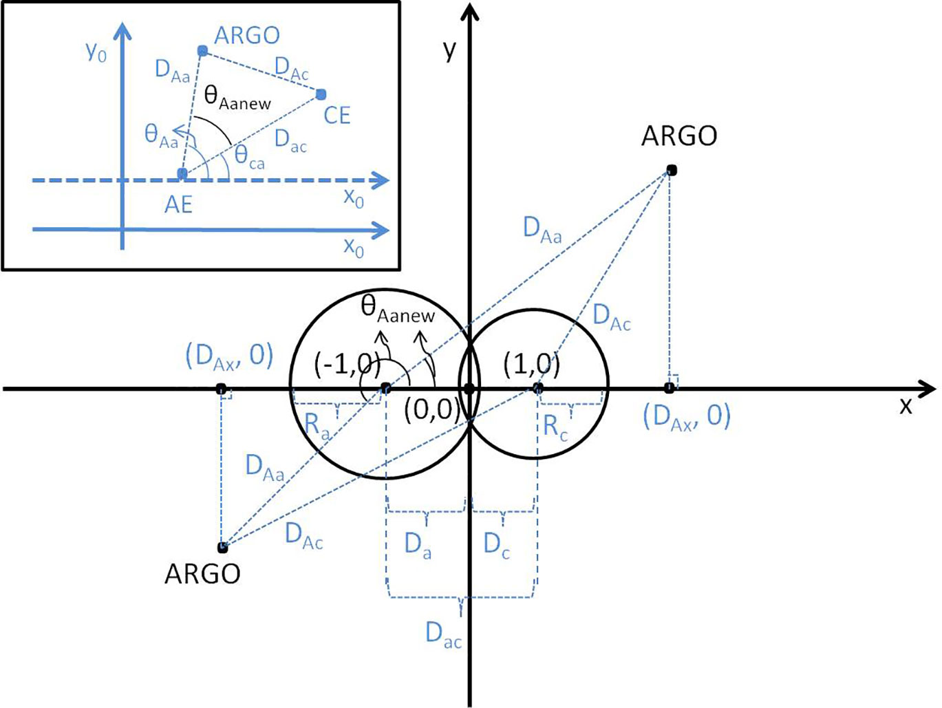
Figure 1 Diagram of the original coordinate system (shown in the northwest box) and new coordinate system for a dipole and corresponding ARGO profiles. Variables written in blue represent values in the original coordinate system.
In total, there were 20,325 OS dipoles and 1,297 CF dipoles with sufficiently close ARGO profiles. This requirement for having nearby ARGO profiles is necessary to enable later 3-D structure analysis of the dipoles. If neighboring ARGO profiles are not required, the numbers of OS and CF dipoles were 72,452 and 4,581, respectively. Figure 2 shows the 72,452 OS dipoles superimposed by fronts in the Southern Indian Ocean.
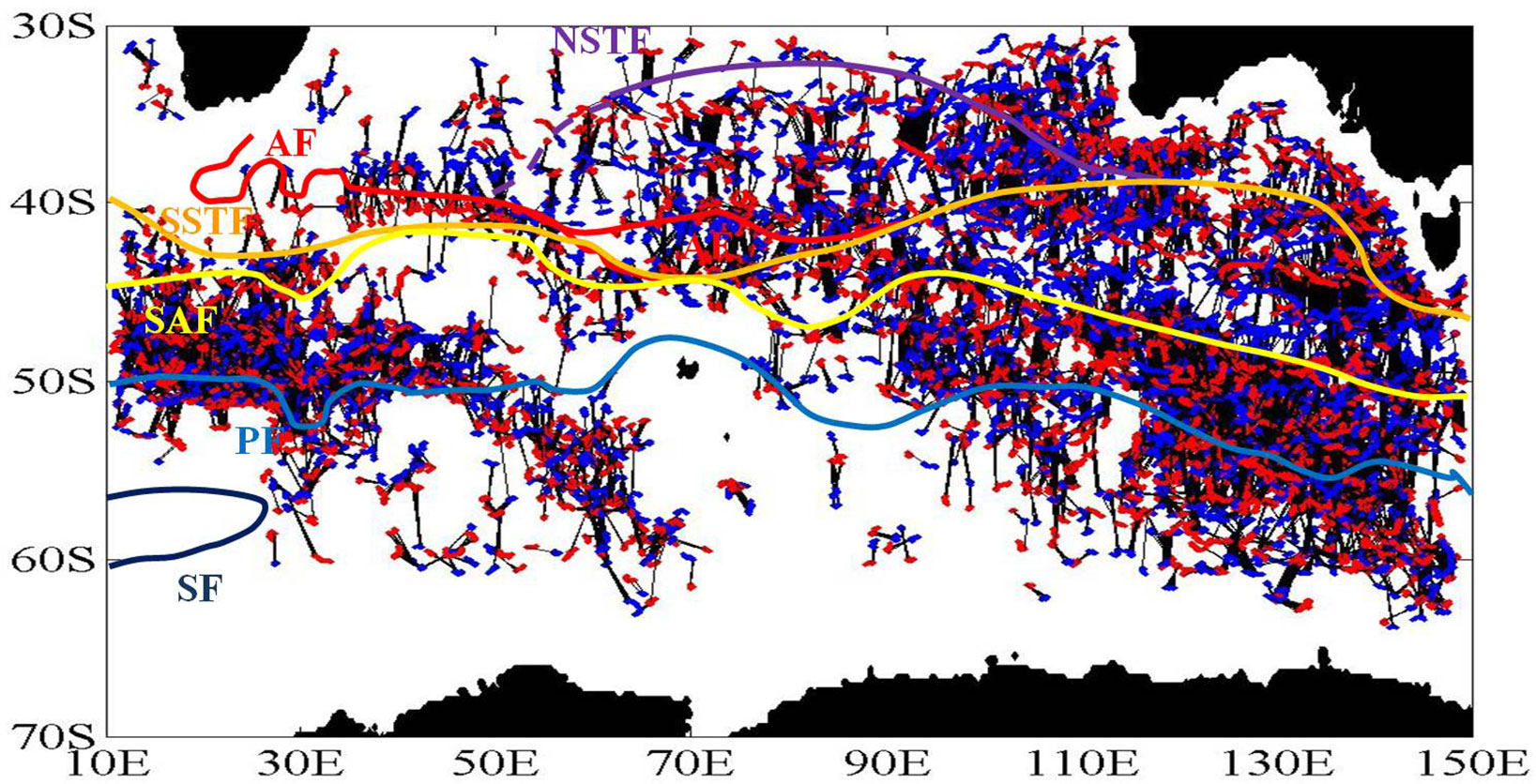
Figure 2 Distribution of OS dipoles without the requirement for a neighboring ARGO profile and fronts in the Southern Indian Ocean. The red dots are AEs, the CEs are shown in blue, and the AE and CE of each dipole are connected by a black line. Fronts (Orsi et al., 1995; Belkin and Gordon, 1996) include the Agulhas Front (AF) (red curve), the northern Subtropical Front (NSTF) (purple curve), the southern Subtropical Front (SSTF) (orange curve), the Subantarctic Front (SAF) (yellow curve), the Polar Front (PF) (blue curve), and the Scotia Front (SF) (dark blue curve).
2.2.2 Simulation of the CF dipole
The numerical experiment in this study used the mixed coordinate HYCOM ocean model (Ansorge and Lutjeharms, 2005), with the KPP parameterization scheme (Bracco et al., 2000). The model domain was a flat-bottomed ocean of 4000 m depth between 35° S and 65° S. The horizontal resolution of the model was 10 km, with 60 vertical levels. To easily initialize the observed temperature and salinity, the pure z-coordinate was adopted in HYCOM. The 60-level vertical coordinate were configured at the geometric proportion of 1.07 with the uppermost level being z=-4 m. The wind stress and thermal forcing were set to zero, and a quasigeostrophic dipole motion in the model was self-induced. In the model, the dipole was initialized by the synthetic T and S fields of the CF dipole. The Lagrangian particle trajectories were computed by using the finite difference method.
3 Results
3.1 Case study of the CF dipole evolution
As outlined in the introduction, a remarkable feature of a dipole is the CF generated between the dipole’s AE and CE. Because this feature may be of significance, the aim of this study is to investigate the role that the CF may play in the subsequent evolution process of the dipole.
The first step is to get an intuitive sense of the evolution process and what influence a CF may have on it. Consequently, a detailed case study of a typical CF dipole was conducted from the sea surface down to 1500 dbar. A dipole that lived just over one month (Jan. 13 - Feb. 14, 2007) with an obvious CF feature was selected and it is shown in Figures 3 and 4 with the SLA contours superimposed on the SSTA and the CHL concentration, respectively. By Jan. 21 (Figures 3B, 4B), a northward flow between the dipole’s AE and CE eddies had gradually developed and the CHL was beginning to be transported northward from the high concentration area to the north of the dipole. By Jan. 29 (Figures 3C, 4C), a low, convex and tongue-like SSTA had developed between the AE and CE and a CF had clearly developed. By Feb. 06 (Figures 3D, 4D), the CF water showed signs of interacting with the CE, and by Feb. 14 (Figures 3E, 4E), the minimum of SSTA and the maximum of CHL concentration were well established within the CE but were beginning to slowly weaken.

Figure 3 Snapshots of the SSTA (color) for a CF dipole with contours of SLA (gray curves) drawn at intervals of 10 cm superimposed. The development and maturity of a CF between the dipole’ AE and CE eddies (A–C), its interaction with the CE (D) and the appearance of the CF water in the CE (E, F). The thick dotted curves are the outermost closed contour of each component eddy, with the arrows indicating the directions of the horizontal geostrophic flow. The triangles labeled ‘A’ and ‘C’, mark the centers of the AE and CE, respectively. Except for the SLA contours, the features for the AE are shown in red, and those for the CE are shown in blue.
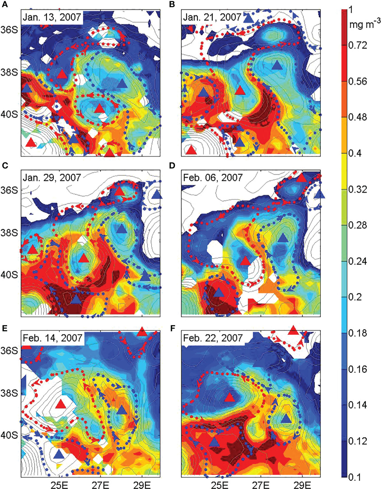
Figure 4 The same as Figure 3 except for the CHL concentration.
In addition to the above analysis on the sea surface, the evolution process in the subsurface domain was further analyzed using the 3-D gridded T and S data described in section 2.1.
Figure 5 shows the potential density distribution on Jan. 24, Feb. 07, and Feb. 14 on the 20 dbar and 300 dbar isobaric surfaces. These three days represent the three stages in the evolution of the dipole: 1) the CF formation, 2) the onset of the CF-dipole interaction, and 3) the mature CF-dipole interaction, respectively. This evolution primarily occurs in the upper layer (see the 20 dbar surfaces in Figures 5A–C) on the northern flank of the dipole (near 38° S). In the first stage, as shown in Figure 5A on Jan. 24, due to the north-south fluctuation of the front where the dipole was located, a low potential density AE and a high potential density CE had appeared. In addition, a CF had formed and presented on the 20 dbar surface as a tongue-like area of higher potential density between the AE and CE, which was due to the existence of the north-south background temperature gradient and the effect of the northward advection between the AE and CE. By the second stage, as shown in Figure 5B on Feb. 07, with the further evolution of the dipole, the CF was a fully developed high potential density center. Concurrently, the CF was beginning to interact with the CE. By the third stage, as shown in Figure 5C on Feb. 14, the CF was fully engaged with the CE. Since cold water had been transported to the northern side of the dipole from between its AE and CE, a cold, high potential density region had formed in the northern flank of the CE, near 38° S. As a result, the low and high potential densities near the centers of the AE and CE, respectively, had returned. During this process, the phase difference between the thermal and dynamic centers that was generated as the CF formed had been eliminated as the CF became fully engaged with the CE. In a previous study of the vertical structure of an Agulhas ring, Souza et al. (2011) found a phase difference between the geostrophic flow and the temperature field. Further, phase differences between SST and Sea Surface Height (SSH) were also found in mesoscale eddies in the North Atlantic and the Southern Ocean (Hausmann and Czaja, 2012). The CF-dipole interaction may be the mechanism that generates this phase difference phenomenon.
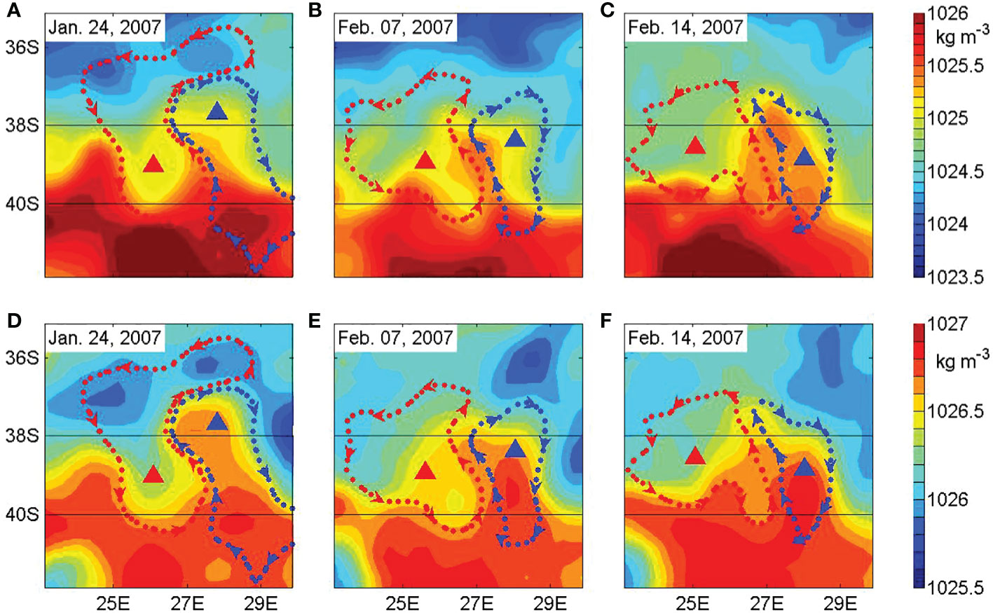
Figure 5 The potential density of the dipole on the isobaric surfaces. The upper row (A–C) is on the 20 dbar surface, and the lower row (D–F) is on the 300 dbar surface. As before, the dotted line is the outermost closed contour of each eddies, the triangles mark the centers of eddies with an ‘A’ and ‘C’ labeling the AE and CE respectively, and the arrows on the dotted lines indicate the directions of the horizontal geostrophic flows. The features for AEs are shown in red, and those for the CEs are shown in blue.
However, in the lower layer, the northern flank of the dipole (see the 300 dbar surfaces in Figures 5D–F) was different from that in the upper layer in that its isopycnals within the CE showed a downward trend. Combining this with the temporal variations in the area, the amplitude, and the average EKE of the CE (not shown), it’s clear that the CE showed a weakening trend after its interaction with the CF.
While the northern flank of the CE was weakening, the isopycnals in the lower layer (300 dbar) rose on the southern flank of the CE near 40° S (Figures 5D–F), which implies that a new north-south frontal fluctuation had enhanced the intensity of the dipole.
Based on the above analysis, the evolution process of the dipole can be summarized as follows: 1) In the upper layer, as the dipole strengthens, a CF is formed between the dipole’s AE and CE, and a phase difference develops between the thermal and dynamic centers of the dipole; 2) The CF water is gradually advected into the CE; 3) Cold water with high CHL concentrations appears within the CE, and the phase difference between the thermal and dynamic centers of the dipole disappears. Concurrently, the lower isopycnals sink, and the CE weakens. It can be seen that the interaction of the dipole with the CF is an important dynamic feature in the evolution of the dipole.
3.2 3-D structure of the CF dipole
In the case study just presented, the CF-dipole interaction generated a high potential density center in the upper layer of the CE component of the CF dipole. If this feature of CF-dipole interaction is universal, it would be expected that high potential density should also occur in the upper layer of the CE in the 3-D synthetic dipole. The structure of CF dipoles was synthesized with that of OS dipoles for comparison using the algorithm described in section 2.2.
The distributions of ARGO profiles contributing to the synthetic results of the OS and CF dipoles in the new coordinate system are shown in Figures 6A, B, respectively. The results of taking the SLA values of points within -2.5≤x ≤ 2.5 and -1.5≤y ≤ 1.5 of the OS and CF dipoles for the Barnes interpolation are shown in Figures 6C, D. From the horizontal geostrophic velocity distributions of the OS and CF dipoles (not shown), it can be seen that the maximum amplitude of the northward geostrophic velocity between the AE and CE of the CF dipole (~20 cm s-1) is stronger than that of the OS dipole (~16 cm s-1). The CF dipole can be regarded as a strengthened OS dipole possessing stronger northward flow. With an appropriate background temperature gradient the flow may have a cold tongue character and becomes the CF structure, and thus the strengthened OS dipole turns to be a CF dipole. A further difference between the CF and OS dipoles is reflected in the distributions of the potential density anomalies. Figures 6E, F are zonal sections of the potential density anomalies along the axis connecting the centers of the AE and CE of the OS and CF dipoles, respectively. The AE in both the CF and OS dipoles has two negative potential density anomaly maxima in the vertical direction, one near 250 dbar and the other near 850 dbar, while the CE in both the CF and OS dipoles has only one positive potential density anomaly maximum near 750 dbar. Therefore, the distributions of the potential density anomaly maxima in the synthetic OS and CF dipoles are analogous to those in the individual synthetic AE and CE in the Southern Indian Ocean (not shown). However, due to there is no CF between the OS dipole’s component eddies, the potential density anomaly maximum as the result of the CF-dipole interaction that appears in the upper layer of the CF dipole’s CE is not present in the OS dipole. Because it’s a synthetic result this maximum reflects the prevailing of the CF-dipole interaction in CF dipoles.
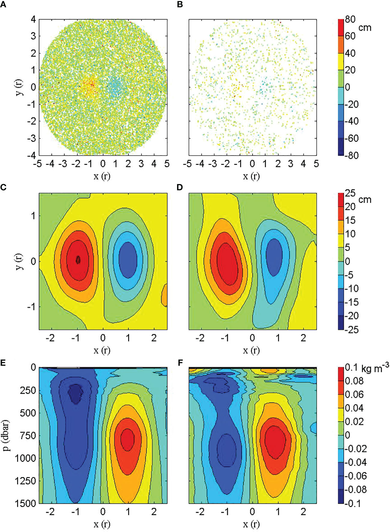
Figure 6 The synthesis of the OS and CF dipoles. The distributions of ARGO profiles around the dipoles used in the synthesis are shown in the new coordinate of x=-5:0.1:5 and y=-4:0.1:4 for (A) the OS dipole and (B) the CF dipole, and the colors represent the values of the SLA. The SLA distributions of both dipoles after the Barnes interpolation are shown in the new coordinate of x=-2.5:0.1:2.5 and y=-1.5:0.1:1.5 for (C) the OS dipole and (D) the CF dipole. Zonal sections of potential density anomalies passing through the central axises of the dipoles are shown for (E) the OS dipole and (F) the CF dipole.
3.3 Statistics of the CF dipole evolution
Although the universality of the CF interaction with the CE of the dipole has been demonstrated from the analysis of the 3-D synthesized dipoles, the temporal characteristics of the interaction process remain to be examined. Because it was observed in the initial CF-dipole interaction case study that CHL entered the CE during the interaction process, the time variation of the CHL concentrations between the centers of AE and CE may intuitively reveal the dynamics of the CF-dipole interaction.
Therefore, a statistical sample was comprised of the CF dipoles not subject to the requirement that a nearby ARGO profile existed while meeting the requirement that both the AE and CE components existed for at least 5 days before and after they paired to form a dipole. Here, we adopted the first time both the squeezing condition and the conditon of the CF existence were met to be the time of dipole formation. A total of 263 dipoles were found that met these requirements. Next, the CHL concentrations on the line between the centers of AE and CE were interpolated onto the normalized distance of 1.
The change in CHL between the dipole’s AE and CE and the temporal evolution of CHL near the centers of the AE and CE around the time of dipole formation are shown in Figures 7A–C, respectively. At that time, the CHL concentration near the center of the AE is at its lowest level, while the CHL concentration near the center of the CE reaches its peak. Simultaneously, the temporal variations of the area and the absolute amplitude of both the AE and CE within the dipole (not shown) reach their peaks around this time. This agrees with the CHL change mechanism for eddies described in Gaube et al. (2014) that when the AE (CE) intensifies, the subsidence (rise) of the isopycnal surface reduces (increases) the nutrients in the euphotic zone, inhibiting (promoting) the growth of phytoplankton. Following the dipole formation phase, the CHL concentration near the center of the CE gradually returns to its level prior to dipole formation. This is because at this stage the intensity of the CE is weakening, and the isopycnals relax leading to the shutoff of the increase of CHL. However, after about two days of weakening the CHL concentration near the center of the CE increases again. Observing the spatial distribution of the CHL at this time, we can find the reason for the second CHL increase. In Figure 7A, high CHL concentration can be found extending from the area centered on x=0.6 where the CF is located to the side of the CE. Therefore, the extension of the high CHL concentration from the location of the CF into the CE following dipole formation confirms the previous prediction of the universal nature of the CF-dipole interaction. In brief, during the entire evolution process described above, the two peaks in CHL in the CE are caused first by the strengthening of the CE and then by the interaction of the CF water with the CE after its formation.
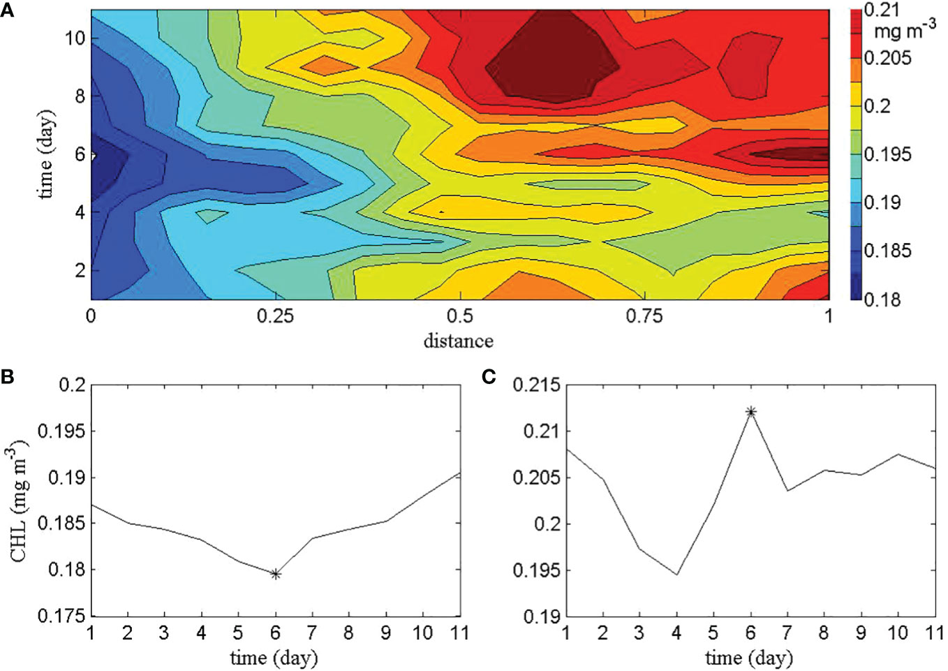
Figure 7 The temporal variations around the time of dipole formation of (A) CHL on the central axis of the dipole, (B) CHL in the center of the AE, and (C) CHL in the center of the CE. The stars in (B, C) mark the minimum and maximum, respectively.
The CF-dipole interaction, which leads to the secondary high CHL concentrations in the CE, may be a new mechanism for the increase of CHL on the north side of the front. As some CEs eventually split from dipoles in the front to the north, the cold and high CHL concentration water from the southern side of the front can be transported northward. The significant meridional transport of water and CHL by mesoscale eddies in the Antarctic Circumpolar Current region (Zhang et al., 2014; Sun et al., 2019; Zhao et al., 2021) may be related to this phenomenon. It should be noted that, either the CHL transport is accomplished by the south to north flow between the AE and CE of a dipole or the northward movement of CEs after separating from the frontal dipoles, the transport by the oceanic dipoles studied in this paper is mainly meridional. This is different from the zonal transport of CHL by nearshore eddies (Feng et al., 2007; Moore et al., 2007; Wang et al., 2018).The structural foundation for the CF-dipole interaction will be addressed in the next subsection using numerical simulation.
3.4 Simulation of the dynamic structure of the CF dipole
From the case study, the 3-D synthesis, and the normalized statistical analysis the importance and universality of the CF-dipole interaction in the temporal evolution of the dipole’s structure have been demonstrated. Nevertheless, a few questions remain: Why is the CF water only entrained into the CE and not the AE? What are the dynamics driving this bias? Is this bias related to differences in the dynamic structure between the AE and CE? To try to answer these questions, this subsection uses the numerical model results to analyze the full 3-D flow field of the dipole. The details of the numerical simulation were described in section 2.2.
In the simulation results, the CE had squeezed west into the middle area of the AE, splitting it into a northern AE and a southern AE, and the CE rotated clockwise with the northern AE (not shown). The paired AE and CE gradually weakened during this process. In order to understand the flow field of the dipole interacting with the CF, the simulation results on day 120 (Figure 8) are used for analysis. Ten particles (Figure 8B) were released in the CF dipole (Figure 8A).
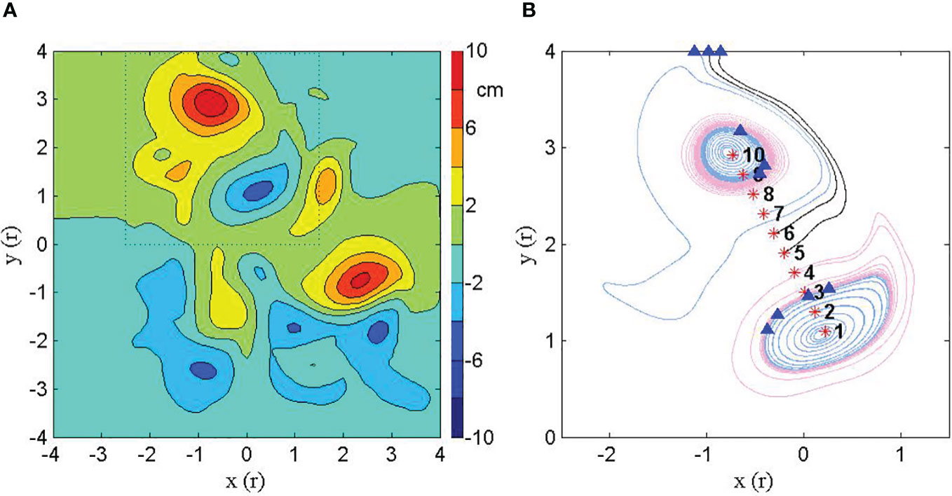
Figure 8 (A) SLA distribution of the dipole on Day 120, with the dipole framed by the dashed line box. (B) 2-D trajectories for particles released on the 50 dbar surface at the 10 equally spaced points between the centers of the AE and CE of the dipole. The track of each particle starts at the red asterisk and ends at the blue triangle. Blue contours indicate that the tracks are divergent while pink contours indicate that the tracks are convergent.
The 2-D Lagrangian particle trajectories for the ten particles released on the 50 dbar isobaric surface between the AE and CE are shown in Figure 8B. The trajectories of particles released near the center of the CE (Particles 1 and 2) are divergent, while the trajectories of the outer two CE particles (Particles 3 and 4) are convergent. Particles 1-4 all remain in the same convergent shear circle within the CE, which have endpoints represented by the four blue triangles. The trajectories of the particles near the center of the AE (Particles 10 and 9) are divergent, while the trajectory of the particle further from the center (Particle 8) is convergent. Particles 8-10 all remain in the same convergent shear circle within the AE, which have endpoints represented by the three blue triangles. The trajectory of the outermost particle (Particle 7) of the AE is divergent and makes one loop around the AE before exiting the dipole. In addition, there are two particles (Particles 5 and 6) between the AE and CE, which pass through the dipole without being entrained by either the AE or the CE.
We further drew the backward and forward trajectories of representative particles in Figure 8B in 3-D space as shown in Figure 9. The trajectories of particles released in the CE are shown in Figures 9B, D and F. In Figure 9B, Particle 1, which represents particles in and around the center of the CE, comes from the sinking divergence of the upper layer near the center, continues to diverge outward, and then diverges and rises on the convergent shear circle. In Figures 9D, F, Particles 3 and 4, which represent peripheral particles of the CE, originate in the sinking convergence of the outer upper layer, and then converge and rise on the convergent shear circle. Figures 9A, C, E draw the trajectories of particles released in the AE. The particles near the center of the AE are represented by Particle 10 (Figure 9A), which originates in the rising divergence of the lower layer near the center, diverges outward, and then sinks into the convergent shear circle. At the place on the flank of the AE is Particle 8 (Figure 9C), which represents particles around the AE center. This particle originates in the rising convergence of the outer lower layer, and then converges and sinks on the convergent shear circle. Particle 7 (Figure 9E), which represents the particles released from the periphery of the AE moves due to the rising divergence of the lower layer and continues to rise. Comparing the 3-D structures of the Lagrangian flow fields of the AE and CE, it is apparent that they are different over their entire extent.
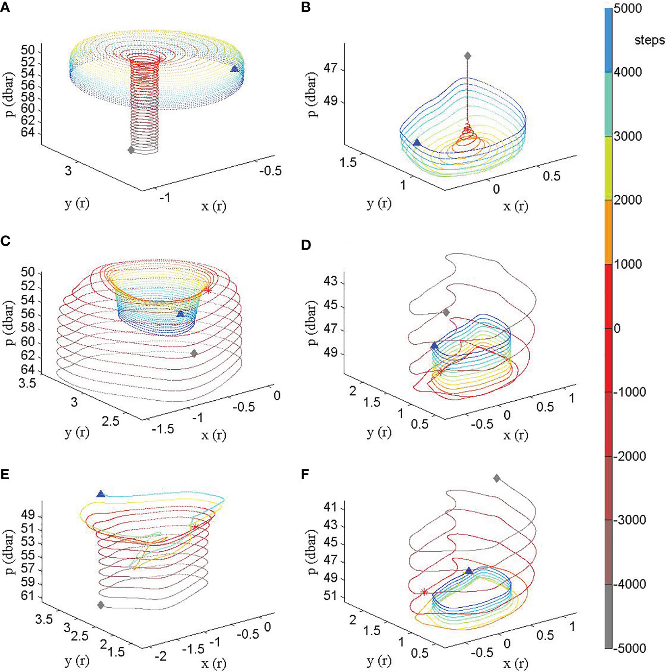
Figure 9 The 3-D trajectories of particles. Particles 10, 8 and 7, which are released in the AE are in the left column graphs from the top to bottom (A, C, E), respectively. Particles 1, 3 and 4, which are released in the CE, are shown in the right column graphs from the top to bottom (B, D, F), respectively. The reverse trajectories originate from the red asterisks, travel at the reverse speeds on each step, and end at the gray diamonds. Each particle’s color gradually changes from gray to red if being viewed in forward direction. The forward trajectories originate from the red asterisks and end at the blue triangles, with the particle’s color gradually changing from red to blue.
On the basis of the Lagrangian analysis, Figure 10 is a schematic diagram of the 3-D structure of the AE and CE components of the CF dipole. The AE is composed of a central circle, which corresponds to a zone of upward divergence, and two outer concentric rings. The inner ring corresponds to a zone of upward convergence, while the outer ring corresponds to a zone of upward divergence. The CE is composed of a central circle with only one concentric ring surrounding it. The Lagrangian trajectories of the CE has the same convergence-divergence behavior as the central circle and the inner annular area ring of the AE, except that they mainly show downward motion instead of upward motion. The radially alternate distribution of ω with opposite directions in the dipole’s CE in this study is consistent with that of an individual CE studied by Nardelli (2013). However, the sinking, rising and sinking from inside to outside of the dipole’s CE in this study are opposite to those of the CE in Nardelli (2013). This difference may be due to the fact that the CE is weakening in this study, while the one in Nardelli (2013) was strengthening, and the vertical flow in a growing eddy is contrary to that of a decaying eddy (de Villiers et al., 2015; Sun et al., 2019).

Figure 10 The schematic diagram of the 3-D structures of the CF dipole’s AE (left) and CE (right). The blue and pink concentric rings represent zones of divergent and convergent particle motions, respectively. The dark red and dark blue circles represent the shear circles upon which particles converge and diverge, respectively. Arrows indicate vertical movements of water and associated divergence or convergence.
Looking at the detailed structures of the CF dipole’s component eddies (Figure 10), the divergence of the outermost concentric ring of the AE prevents the CF water from being entrained into the AE, while the lack of this divergent ring and the convergence in the outmost ring of the CE promotes the entrainment of the CF water into the CE. As a result, the problem of the biased movement of the CF water raised in the previous sections has been finally resolved.
According to Klein and Lapeyre (2009), the interior of a mesoscale eddy is dominated by vorticity and its vertical motion is caused by the rise or fall of the isopycnals, while the area surrounding the eddy is dominated by deformation and its vertical motion is driven by temporal changes in sea surface density. Owing to our purpose, only Lagrangian movements of the inner areas of the AE and CE and the middle area between the two component eddies of the CF dipole have been presented. Particle movements having four alternating positive and negative extrema of ω in the Eulerian framework, are not shown, as they are the same as that studied by Ni et al. (2020).
4 Conclusion
Prior work presented some characteristics of the 3-D structure of dipoles (Ni et al., 2020; Yin et al., 2020). However, the CF, a remarkable feature of many dipoles, which had not been previously well studied, may play an important role in the structural evolution of dipoles.
In this paper, a case study was conducted, which provided a hint that the interaction of a CF with the CE within a dipole was a key process in the structural evolution of the dipole. After giving a concise definition of the CF dipole, observed CF dipoles were used to build a synthetic structure of a dipole with the CF. These CF dipoles were then used to normalize the evolution process of the CF dipoles. These studies verified the universality of the CF-dipole interaction. We investigated the mechanism of the interaction through the simulation of the synthetic data for the CF dipole and a Lagrangian analysis of particles released within the dipole. This Lagrangian analysis revealed the structural foundation of the CF-dipole interaction.
We found that through its interaction with the dipole, the CF changed the structure of the dipole. The appearance of the CF created a positional difference between the thermal and dynamic centers of the dipole. However, the CF-dipole interaction caused the thermal and dynamic centers of the CE to coincide, forming a high positive density anomaly in the upper layer of the CE. The appearance and the interaction of the CF with the dipole studied here may provide a mechanism for the generation and the elimination of the phase difference of eddies. We also found that the CF-dipole interaction entrained not only cold water but also high CHL water into the CE of the dipole. Therefore, the CF-dipole interaction is the driver for the secondary onset and maintenance of the high CHL concentrations in the upper layer of the dipole’s CE.
We sought the root reason for the CF-dipole interaction and found that it lay in the respective detailed structural characteristics of the dipole’s AE and CE. From the inside to the outside, the AE has a three-zone structure of divergence, convergence and divergence, while the CE has only a two-zone structure of divergence and convergence. Therefore, only the CE’s outermost zone is convergent and thus only the CE can entrain CF water, which enters between the dipole’s AE and CE. This is the cause of the remarkable bias in the CF interaction with the CE, how the detailed structures of the two eddies contribute to the dipole linkup, and the foundation of the CF-dipole interaction.
The critical role of the CF in the evolution of a dipole structure should be noticed. Meanwhile, the high CHL concentration water that is entrained into the CE during the evolving interaction process enhances the ecological effects of mesoscale eddies. However, this study only focuses on the role of the CF on the dipole during its decaying stage, which is the period of CF entrainment. Future work should consider the structural characteristics of the dipole during its strengthening stage to get a complete picture of the dipole evolution.
Data availability statement
The original contributions presented in the study are included in the article/supplementary material. Further inquiries can be directed to the corresponding author.
Author contributions
GG and QY conceived and designed the research. GW guided the specific research methods. QY conducted the data analysis and wrote the original draft. CX, GG, and RS participated in the revision of the manuscript. QY, GG, and GW provided the funding for the work. All authors read and approved the submitted version.
Funding
This work was sponsored by the National Key Research and Development Program of China (2019YFC1510100 and 2019YFC1510100), the General Program of National Natural Science Foundation of China (NSFC-41276197) and the National Natural Science Foundation of China (grants 42030405).
Acknowledgments
The authors sincerely thank Zhumin Lu at South China Sea Institute of Oceanology for the help on the model simulation.
Conflict of interest
The authors declare that the research was conducted in the absence of any commercial or financial relationships that could be construed as a potential conflict of interest.
Publisher’s note
All claims expressed in this article are solely those of the authors and do not necessarily represent those of their affiliated organizations, or those of the publisher, the editors and the reviewers. Any product that may be evaluated in this article, or claim that may be made by its manufacturer, is not guaranteed or endorsed by the publisher.
References
Ansorge I. J., Lutjeharms J. R. E. (2005). Direct observations of eddy turbulence at a ridge in the southern ocean. Geophysical Res. Lett. 32, L14603. doi: 10.1029/2005GL022588
Belkin I. M., Gordon A. L. (1996). Southern ocean fronts from the Greenwich meridian to Tasmania. J. Geophysical Research: Oceans 101 (C2), 3675–3696. doi: 10.1029/95JC02750
Bettencourt J. H., López C., Hernández-García E. (2012). Oceanic three-dimensional Lagrangian coherent structures: a study of a mesoscale eddy in the benguela upwelling region. Ocean Model. 51, 73–83. doi: 10.1016/j.ocemod.2012.04.004
Bracco A., Provenzale A., Scheuring I. (2000). Mesoscale vortices and the paradox of the plankton. Proc. R. Soc. London. Ser. B: Biol. Sci. 267 (1454), 1795–1800. doi: 10.1098/rspb.2000.1212
Capet X., Klein P., Hua B. L., Lapeyre G., McWilliams J. C. (2008). Surface kinetic energy transfer in surface quasi-geostrophic flows. J. Fluid Mechanics 604, 165–174. doi: 10.1017/S0022112008001110
Chaigneau A., Le Texier M., Eldin G., Grados C., Pizarro O. (2011). Vertical structure of mesoscale eddies in the eastern south pacific ocean: a composite analysis from altimetry and argo profiling floats. J. Geophysical Research: Oceans 116, C11025. doi: 10.1029/2011JC007134
Chelton D. B., Gaube P., Schlax M. G., Early J. J., Samelson R. M. (2011a). The influence of nonlinear mesoscale eddies on near-surface oceanic chlorophyll. Science 334 (6054), 328–332. doi: 10.1126/science.1208897
Chelton D. B., Schlax M. G., Samelson R. M. (2011b). Global observations of nonlinear mesoscale eddies. Prog. Oceanography 91 (2), 167–216. doi: 10.1016/j.pocean.2011.01.002
de Villiers S., Siswana K., Vena K. (2015). In situ measurement of the biogeochemical properties of southern ocean mesoscale eddies in the southwest Indian ocean, April 2014. Earth System Sci. Data 7, 415–422. doi: 10.5194/essd-7-415-2015
Ducet N., Le Traon P. Y., Reverdin G. (2000). Global high-resolution mapping of ocean circulation from TOPEX/Poseidon and ERS-1 and-2. J. Geophysical Research: Oceans 105 (C8), 19477–19498. doi: 10.1029/2000jc900063
Durgadoo J. V., Ansorge I. J., de Cuevas B. A., Lutjeharms J. R. E., Coward A. C. (2011). Decay of eddies at the south-West Indian ridge. South Afr. J. Sci. 107 (11-12), 14–23. doi: 10.4102/sajs.v107i11/12.673
Falkowski P. G., Ziemann D., Kolber Z., Bienfang P. K. (1991). Role of eddy pumping in enhancing primary production in the ocean. Nature 352 (6330), 55–58. doi: 10.1038/352055a0
Faure V., Arhan M., Speich S., Gladyshev S. (2011). Heat budget of the surface mixed layer south of Africa. Ocean Dynamics 61 (10), 1441–1458. doi: 10.1007/s10236-011-0444-1
Feng M., Majewski L. J., Fandry C. B., Waite A. M. (2007). Characteristics of two counter-rotating eddies in the leeuwin current system off the Western Australian coast. Deep Sea Res. Part II: Topical Stud. Oceanography 54 (8), 961–980. doi: 10.1016/j.dsr2.2006.11.022
Frenger I. (2013). On Southern Ocean eddies and their impacts on biology and the atmosphere. [dissertation/doctor's thesis]. [Zürich]: Eidgenössische Technische Hochschule Zürich.
Frenger I., Münnich M., Gruber N., Knutti R. (2015). Southern ocean eddy phenomenology. J. Geophysical Research: Oceans 120 (11), 7413–7449. doi: 10.1002/2015JC011047
Gaube P., McGillicuddy D. J., Chelton D. B., Behrenfeld M. J., Strutton P. J. (2014). Regional variations in the influence of mesoscale eddies on near-surface chlorophyll. J. Geophysical Research: Oceans 119, 8195–8220. doi: 10.1002/2014jc010111
Gaube P., Chelton D. B., Samelson R. M., Schlax M. G., O'Neill L. W. (2015). Satellite observations of mesoscale eddy-induced ekman pumping. J. Phys. Oceanography 45 (1), 104–132. doi: 10.1175/jpo-d-14-0032.1
Guidi L., Calil P. H. R., Duhamel S., Björkman K. M., Doney S. C., Jackson G. A., et al. (2012). Does eddy-eddy interaction control surface phytoplankton distribution and carbon export in the North Pacific Subtropical Gyre?? Journal of Geophysical Research: Biogeosciences 117 (G02024). doi: 10.1029/2012JG001984
Hakim G. J., Snyder C., Muraki D. J. (2002). A new surface model for cyclone–anticyclone asymmetry. J. Atmospheric Sci. 59 (16), 2405–2420. doi: 10.1175/1520-0469(2002)059<2405:ANSMFC>2.0.CO;2
Hausmann U., Czaja A. (2012). The observed signature of mesoscale eddies in sea surface temperature and the associated heat transport. Deep Sea Res. Part I: Oceanographic Res. Papers 70, 60–72. doi: 10.1016/j.dsr.2012.08.005
Held I. M., Pierrehumbert R. T., Garner S. T., Swanson K. L. (1995). Surface quasi-geostrophic dynamics. J. Fluid Mechanics 282, 1–20. doi: 10.1017/S0022112095000012
Hughes C. W., Miller P. I. (2017). Rapid water transport by long-lasting modon eddy pairs in the southern midlatitude oceans. Geophysical Res. Lett. 44, 12375–12384. doi: 10.1002/2017GL075198
Jayne S. R., Marotzke J. (2002). The oceanic eddy heat transport. J. Phys. Oceanography 32 (12), 3328–3345. doi: 10.1175/1520-0485(2002)032<3328:TOEHT>2.0.CO;2
Klein P., Lapeyre G. (2009). The oceanic vertical pump induced by mesoscale and submesoscale turbulence. Annu. Rev. Mar. Sci. 1 (1), 351–375. doi: 10.1146/annurev.marine.010908.163704
Lee D. (2018). High concentration chlorophyll a rings associated with the formation of intrathermocline eddies. Limnology Oceanography 63 (6), 2806–2814. doi: 10.1002/lno.11010
Lévy M., Franks P. J. S., Smith K. S. (2018). The role of submesoscale currents in structuring marine ecosystems. Nat. Commun. 9 (1), 4758. doi: 10.1038/s41467-018-07059-3
Liu L., Xue H. J., Sasaki H. (2019). Reconstructing the ocean interior from high-resolution Sea surface information. J. Phys. Oceanography 49 (12), 3245–3262. doi: 10.1175/JPO-D-19-0118.1
Machu E., Ferret B., Garçon V. (1999). Phytoplankton pigment distribution from SeaWiFS data in the subtropical convergence zone south of Africa: a wavelet analysis. Geophysical Res. Lett. 26 (10), 1469–1472. doi: 10.1029/1999GL900256
McGillicuddy D. J., Anderson L. A., Bates N. R., Bibby T., Buesseler K. O., Carlson C. A., et al. (2007). Eddy/Wind interactions stimulate extraordinary mid-ocean plankton blooms. Science 316 (5827), 1021–1026. doi: 10.1126/science.1136256
McGillicuddy D. J., Robinson A. R. (1997). Eddy-induced nutrient supply and new production in the Sargasso Sea. Deep Sea Res. Part I: Oceanographic Res. Papers 44 (8), 1427–1450. doi: 10.1016/S0967-0637(97)00024-1
McGillicuddy D. J., Robinson A. R., Siegel D. A., Jannasch H. W., Johnson R., Dickey T. D., et al. (1998). Influence of mesoscale eddies on new production in the Sargasso Sea. Nature 394 (6690), 263–266. doi: 10.1038/28367
Moore T. S., Matear R. J., Marra J., Clementson L. (2007). Phytoplankton variability off the Western Australian coast: mesoscale eddies and their role in cross-shelf exchange. Deep Sea Res. Part II: Topical Stud. Oceanography 54 (8), 943–960. doi: 10.1016/j.dsr2.2007.02.006
Nardelli B. B. (2013). Vortex waves and vertical motion in a mesoscale cyclonic eddy. J. Geophysical Research: Oceans 118, 5609–5624. doi: 10.1002/jgrc.20345
Nencioli F., Kuwahara V. S., Dickey T. D., Rii Y. M., Bidigare R. R. (2008). Physical dynamics and biological implications of a mesoscale eddy in the lee of hawai’i: cyclone opal observations during e-flux III. Deep Sea Res. Part II: Topical Stud. Oceanography 55 (10-13), 1252–1274. doi: 10.1016/j.dsr2.2008.02.003
Ni Q. B., Zhai X. M., Wang G. H., Hughes C. (2020). Widespread mesoscale dipoles in the global ocean. J. Geophysical Research: Oceans 125, e2020JC016479. doi: 10.1029/2020JC016479
Orsi A. H., Iii T. W., Nowlin W. D. (1995). On the meridional extent and fronts of the Antarctic circumpolar current. Deep Sea Res. Part I Oceanographic Res. Papers 42 (5), 641–673. doi: 10.1016/0967-0637(95)00021-W
Pidcock R., Martin A., Allen J., Painter S. C., Smeed D. (2013). The spatial variability of vertical velocity in an Iceland basin eddy dipole. Deep Sea Res. Part I: Oceanographic Res. Papers 72, 121–140. doi: 10.1016/j.dsr.2012.10.008
Prants S. V., Ponomarev V. I., Budyansky M. V., Uleysky M. Y., Fayman P. A. (2015). Lagrangian Analysis of the vertical structure of eddies simulated in the Japan basin of the Japan/East Sea. Ocean Model. 86, 128–140. doi: 10.1016/j.ocemod.2014.12.010
Santiago-García M. W., Parés-Sierra A. F., Trasviña-Castro A. (2019). Dipole-wind interactions under gap wind jet conditions in the gulf of tehuantepec, Mexico: a surface drifter and satellite database analysis. PloS One 14 (12), e0226366. doi: 10.1371/journal.pone.0226366
Siegel D. A., Peterson P., McGillicuddy D. J., Maritorena S., Nelson N. B. (2011). Bio-optical footprints created by mesoscale eddies in the Sargasso Sea. Geophysical Res. Lett. 38, L13608. doi: 10.1029/2011gl047660
Souza J. M. A. C., de Boyer Montégut C., Cabanes C., Klein P. (2011). Estimation of the agulhas ring impacts on meridional heat fluxes and transport using ARGO floats and satellite data. Geophysical Res. Lett. 38, L21602. doi: 10.1029/2011GL049359
Sun W. J., Dong C. M., Tan W., He Y. J. (2019). Statistical characteristics of cyclonic warm-core eddies and anticyclonic cold-core eddies in the north pacific based on remote sensing data. Remote Sens. 11 (2), 208. doi: 10.3390/rs11020208
Viúdez A. (2018). Two modes of vertical velocity in subsurface mesoscale eddies. J. Geophysical Research: Oceans 123, 3705–3722. doi: 10.1029/2017JC013735
Wang G. H., Chen D. K., Su J. L. (2006). Generation and life cycle of the dipole in the south China Sea summer circulation. J. Geophysical Research: Oceans 111, C06002. doi: 10.1029/2005JC003314
Wang Y., Zhang H., Chai F., Yuan Y. (2018). Impact of mesoscale eddies on chlorophyll variability off the coast of Chile. PloS One 13, e0203598. doi: 10.1371/journal.pone.0203598
Williams R. G., Follows M. J. (1998). Eddies make ocean deserts bloom. Nature 394 (6690), 228–229. doi: 10.1038/28285
Xu G. J., Dong C. M., Liu Y., Gaube P., Yang J. S. (2019). Chlorophyll rings around ocean eddies in the north pacific. Sci. Rep. 9 (1), 2056. doi: 10.1038/s41598-018-38457-8
Xu C., Shang X. D., Huang R. X. (2014). Horizontal eddy energy flux in the world oceans diagnosed from altimetry data. Sci. Rep. 4, 5316. doi: 10.1038/srep05316
Yin H. Q., Dai H. J., Zhang W. M., Zhang X. Y., Wang P. Q. (2020). Demonstration of the refined three-dimensional structure of mesoscale eddies and computational error estimates via Lagrangian analysis. Acta Oceanologica Sin. 39 (7), 146–164. doi: 10.1007/s13131-020-1619-8
Zhai P., Bower A. (2013). The response of the red Sea to a strong wind jet near the tokar gap in summer. J. Geophysical Research: Oceans 118, 422–434. doi: 10.1029/2012JC008444
Zhang Z. G., Qiu B. (2020). Surface chlorophyll enhancement in mesoscale eddies by submesoscale spiral bands. Geophysical Res. Lett. 47, e2020GL088820. doi: 10.1029/2020GL088820
Zhang Z. G., Qiu B., Klein P., Travis S. (2019). The influence of geostrophic strain on oceanic ageostrophic motion and surface chlorophyll. Nat. Commun. 10 (1), 2838. doi: 10.1038/s41467-019-10883-w
Zhang Z. W., Tian J. W., Qiu B., Zhao W., Chang P., Wu D. X., et al. (2016). Observed 3D structure, generation, and dissipation of oceanic mesoscale eddies in the south China Sea. Sci. Rep. 6, 24349. doi: 10.1038/srep24349
Zhang Z. G., Wang W., Qiu B. (2014). Oceanic mass transport by mesoscale eddies. Science 345 (6194), 322–324. doi: 10.1126/science.1252418
Zhang Z. G., Zhang Y., Wang W., Huang R. X. (2013). Universal structure of mesoscale eddies in the ocean. Geophysical Res. Lett. 40 (14), 3677–3681. doi: 10.1002/grl.50736
Keywords: filament, mesoscale eddy dipole, interaction, structure, Lagrangian trajectory, chlorophyll
Citation: Yang Q, Wang G, Xu C, Gao G and Sun R (2023) The influence of cold filaments on the evolution of dipole structures. Front. Mar. Sci. 10:1113993. doi: 10.3389/fmars.2023.1113993
Received: 02 December 2022; Accepted: 29 May 2023;
Published: 15 June 2023.
Edited by:
Xueming Zhu, Southern Marine Science and Engineering Guangdong Laboratory (Zhuhai), ChinaReviewed by:
Yuntao Wang, Ministry of Natural Resources, ChinaChunhua Qiu, Sun Yat-sen University, China
Copyright © 2023 Yang, Wang, Xu, Gao and Sun. This is an open-access article distributed under the terms of the Creative Commons Attribution License (CC BY). The use, distribution or reproduction in other forums is permitted, provided the original author(s) and the copyright owner(s) are credited and that the original publication in this journal is cited, in accordance with accepted academic practice. No use, distribution or reproduction is permitted which does not comply with these terms.
*Correspondence: Guoping Gao, Z3BnYW9Ac2hvdS5lZHUuY24=