 Guancheng Li1,2,3
 Lijing Cheng1,3*
 Yuying Pan1,3
 Gongjie Wang4
 Hailong Liu1,5
 Jiang Zhu1,3Bin Zhang6Huanping Ren6Xutao Wang2
- 1Institute of Atmospheric Physics, Chinese Academy of Sciences, Beijing, China
- 2Eco-Environmental Monitoring and Research Center, Pearl River Valley and South China Sea Ecology and Environment Administration, Ministry of Ecology and Environment, Guangzhou, China
- 3Center for Ocean Mega-Science, Chinese Academy of Sciences, Qingdao, China
- 4People’s liberation Army (PLA) 31526 Troops, Beijing, China
- 5State Key Laboratory of Numerical Modeling for Atmospheric Sciences and Geophysical Fluid Dynamics (LASG), Institute of Atmospheric Physics, Chinese Academy of Sciences, Beijing, China
- 6Institute of Oceanology, Chinese Academy of Sciences, Qingdao, China
A gridded salinity dataset with high resolution is essential for investigating global ocean salinity variability and understanding its role in climate and the ocean ecosystem. In this study, a new version of the Institute of Atmospheric Physics gridded salinity dataset with a higher resolution (0.5° by 0.5°) is provided by using a revised ensemble optimal interpolation scheme with a dynamic ensemble. The performance of this dataset is evaluated using “subsample test” and the high-resolution satellite-based data. Compared with the previous 1° by 1° resolution IAP product, the new dataset is more capable of representing regional salinity changes with the meso-scale and small-scale signals (i.e., in the coastal and boundary currents regions), meanwhile, maintains the large-scale structure and variability. Therefore, the new dataset complements the previous data product. Besides, the new dataset is compared with in situ observations and several international salinity products for the salinity multiscale variabilities and patterns. The comparison shows the smaller magnitude of mean difference and Root-mean-square deviation (RMSD) in basin scale for the new dataset, some differences in strength and fine structure of the “fresh gets fresher, salty gets saltier” surface and subsurface salinity pattern amplification trends from 1980 to 2017, a broad similarity for the salinity changes associated with El Niño-Southern Oscillation (ENSO) and a consistent salinity dipole mode in the tropical Indian Ocean (S-IOD). These results support the future use of gridded salinity data.
1 Introduction
Ocean salinity, as one of the fundamental properties of ocean water, has important implications for the global ocean climate system and ecosystem. For example, the long-term changes in the surface and subsurface salinity are of worldwide concern, as they are ideal indicators of an intensified global water cycle (Durack and Wijffels, 2010; Rhein et al., 2013; Cheng et al., 2020). Furthermore, salinity contributes to the intensity of upper ocean stratification, and thus modulates the vertical oceanic exchanges and large-scale ocean circulation processes, such as the thermohaline circulation in the North Atlantic (Collins et al., 2013; Rahmstorf et al., 2015). The importance of salinity is also highlighted by its role in changes in marine productivity, through the modulation of the spatio-temporal structure of water stratification (Greene et al., 2012), or influencing the adaptation of marine creatures (Ross and Behringer, 2019). Therefore, it is important to investigate salinity variability to understand its role in climate change.
Estimating ocean salinity change is challenging due to the sparse distribution of salinity data and instrumental bias, mainly before the Argo era (Durack, 2015). Since 2005, the Argo observation network has provided more than 300,000 salinity profiles per year, and has achieved near-global coverage since 2007 (Roemmich et al., 2009). Some mainstream data centers publish their salinity products and update them continuously, aiming to provide more accurate estimates of the ocean state, including objective analyses with long time coverage (i.e., the EN dataset from the UK Met Office Hadley Centre) (Good et al., 2013) and Argo-based products, such as the Scripps Institution of Oceanography (SCRIPPS) dataset (Roemmich and Gilson, 2009), the Japanese Agency for Marine-Earth Science and Technology (JAMSTEC) dataset (Hosoda et al., 2008), and the Global Ocean Argo gridded dataset (BOA-Argo) (Lu et al., 2018). Furthermore, advanced data assimilation technologies allow the combination of multiple sources of observations and models, providing a complete three-dimensional salinity field in a physically consistent manner, for instance, the Ocean Reanalysis System (ORA) (Balmaseda et al., 2013) from the European Center for Medium-Range Weather Forecasts (ECMWF) and the Simple Ocean Data Assimilation (SODA) (Carton et al., 2018) from the University of Maryland. These products have been widely used to investigate the salinity variability and model simulations in previous studies (Xue et al., 2017; Carton et al., 2019). For example, the imprints of interdecadal and multidecadal variabilities of sea surface salinity (SSS) as an indicator of change in the hydrological cycle in recent decades has been explored using several salinity datasets, such as Durack and Wijffels (2010) (named DW10), Skliris et al. (2014); Li et al. (2016) using EN4, Vinogradova and Ponte (2017) using the ECCO estimate, and Cheng et al. (2020) using IAP. El Ninão-Southern Oscillation (ENSO) is the dominant mode of variability at interannual scale in the global ocean and the salinity change in the tropical Pacific has been reported to closely correlate the characteristics of the ENSO cycle (Roemmich and Gilson, 2011; Zhu et al., 2014; Zhi et al., 2019). The salinity changes can also affect the upper ocean temperature and the evolution of ENSO by modulating the upper stratification in the Pacific Ocean (Zheng and Zhang, 2015). Previous studies indicate that the ENSO-related salinity variability and its role during the Argo era are well illustrated by Argo-based products, such as the SCRIPPS and JAMSTEC datasets (Roemmich and Gilson, 2011; Zheng and Zhang, 2015). The JAMSETC analysis has also been used to investigate the formation and propagation of subsurface salinity anomalies and water masses in the North Pacific Ocean (Qiu and Chen, 2012; Yan et al., 2013; Katsura et al., 2019). The advantages of these datasets have been demonstrated in specific applications, but few studies have compared them.
Of considerable interest is the comparison of multiscale salinity changes among different salinity products, as they lead to uncertainties in the salinity variability. For instance, the long-term amplification of global salinity contrast, either at the sea surface or the subsurface layer, has been estimated by several studies, but with large discrepancies in the rates of trends (Hosoda et al., 2009; Durack et al., 2012; Skliris et al., 2014; Jan et al., 2018). In the study of Cheng et al. (2020), the estimates of the basin means of the upper-2000 m salinity changes in different salinity datasets demonstrated the substantial differences, particularly in the Southern Ocean and before the Argo era. These disparities can be attributed to various factors, such as quality control procedures, bias correction schemes, choice of climatology, the mapping methods used to fill the data gaps, and so on (Abraham et al., 2013; Boyer et al., 2016; Cheng et al., 2020). Since the beginning of the Argo period, the quality of salinity data has substantially improved due to advanced observations and technologies. Multiple salinity products have consistently revealed a notable vertical contrast, with an increase in salinity in the upper 200 m layer and freshening within the 200-600 m layer in the past decade (Li et al., 2019). However, substantial discrepancies between various Argo-based salinity products are still found in the subsurface North Atlantic and Southern oceans (Liu et al., 2020). Therefore, comparison of regional and global salinity variability between all the available salinity products is still an important issue in salinity research.
Recently, a new version of the salinity gridded dataset from the Institute of Atmospheric Physics (IAP) with a horizontal resolution of 1°×1° (IAP-1) has been released and evaluated (Cheng et al., 2020). A large number of salinity observations over the 1960-2020 period are also found in Northwest Pacific, Northwest Atlantic, and some coastal regions (Figure S1). On this basis, the goal of this study is to explore the possibility to increase the spatial resolution (given the fact that there are many places with dense observations), and improve the performance along the coastline and boundary regions. The new version of the salinity gridded dataset provided in this study has an improved horizontal resolution of 0.5°×0.5° (named IAP-05) (Table 1). The mapping scheme for the IAP-05 dataset and the salinity data used for comparison will be described in section 2.
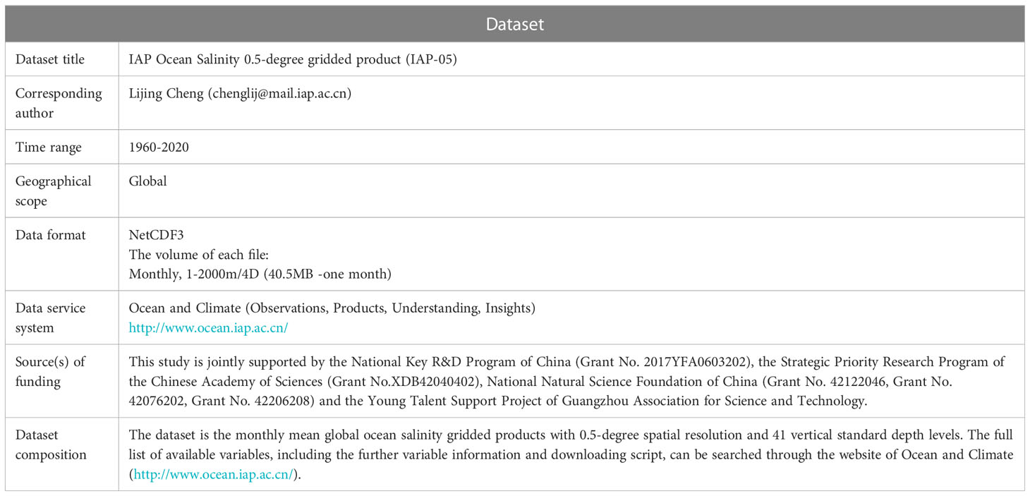
Table 1 IAP ocean salinity 0.5-degree gridded product (IAP-05).
In section 3, we first evaluate the quality of IAP-05 dataset and its uncertainty using a subsample test. The new dataset is also validated by in situ observations and independent observations, including hydrographic observations and satellite products. A comparison of the global and regional salinity variability is then conducted to examine the consistency of the new dataset with other available products. Finally, a discussion is given in section 4.
2 Data and methods
2.1 Mapping method
The mapping method is based on the ensemble optimal interpolation with a dynamic ensemble (ENOI-DE) scheme proposed by Cheng and Zhu (2016). This approach has been applied in the reconstruction of the historical subsurface salinity and temperature fields with 1°×1° horizontal resolution (Cheng et al., 2017; Cheng et al., 2020).
The source of ocean salinity observations is the World Ocean Database (WOD) of historical hydrographic profiles (Garcia et al., 2018). The erroneous profiles have been removed using the quality control procedure provided by WOD18, which has been widely used in the ocean subsurface dataset. The WOD quality flags include the flags for entire cast as a function of variable and flags on individual observations (Garcia et al., 2018). All the salinity profiles have their monthly climatology averaged from 1990 to 2010 subtracted to obtain the salinity anomaly field. Considering the design of the proposed mapping algorithm, the anomaly profiles were then averaged into their horizontal 0.5°×0.5° gridded means for each month and 41 vertical standard depth levels (same as Cheng et al. (2020)). Given the slowness of ocean temporal variation, the salinity observations in different levels were combined to infill the data gaps within a certain time window, which uses the temporal bins (before and after) increasing from 3 months at the surface to 18 months at 2000 m.
In the temperature/salinity reconstruction of the IAP gridded dataset with 1° horizontal resolution (named IAP-1), the Coupled Model Inter-comparison Project Phase 5 (CMIP5) simulations (Taylor et al., 2012) were used to provide a dynamic ensemble (N > 30) of the model background and its spatial covariance (Cheng and Zhu, 2016). One of its advantages is that it provides an improved estimate on the error covariance, that is the major source of information in propagating the information from observed regions to regions with data gaps. However, the previous approach used in IAP-1 relies on the 1°×1° horizontal resolution models in CMIP5 thus not applicable in higher resolution reconstruction.
Here we used a new ensemble of the high-resolution model outputs (N = 26) from high-resolution model simulations and ocean reanalyses, including the High Resolution Model Intercomparison Project (HighResMIP) simulations for CMIP6 (N = 20) (Haarsma et al., 2016), LASG/IAP Climate system Ocean Model version 2.0 (LICOM 2.0) from China (N = 1) (Yu et al., 2012) and Geophysical Fluid Dynamics Laboratory Coupled Climate Model version 4 (GFDL-CM4) (Held et al., 2019) from the United States (N = 1), the fifth generation of climate model of the Institute for Numerical Mathematics (INM-CM5-0) from Russian (N = 1) (Volodin et al., 2017) and three members of Euro-Mediterranean Center for Climate Change (CMCC) Historical Ocean Reanalysis system (CHOR) (Yang et al., 2017) from Italy (N = 3), which use different atmospheric forcings and/or different assimilation methods.
The HighResMIP is one of the CMIP6 endorsed MIPs and it incorporates the model resolution that ranges from typical CMIP6 resolutions of 100 km to higher resolutions of 8~25 km in the ocean (Roberts et al., 2020). LICOM is the eddy-revolving ocean model with nearly global coverage in longitude-latitude grids (i.e., without the Arctic Ocean). GFDL-CM4 is the latest generation of the high-resolution GFDL model for CMIP6 and outperforms the previous GFDL model components (i.e., GFDL-CM3 for CMIP5; CM2.6: eddy-revolving model). Both models can capture the large-scale features of the ocean state, as well as the small-scale and mesoscale activity. Furthermore, they show a better representation along the coastline and boundary regions. INM-CM5-0 is an evolutionary upgraded generation for CMIP6 with a modified dynamical core and two times higher resolution than previous version INM-CM4. More detailed information on the selected members is presented in Tables 2, 3. This new covariance statistic with a dynamic ensemble of multiple sources provides a better representation of the error covariance and can minimize the potential impact of model bias in each individual model through the optimal interpolation process.
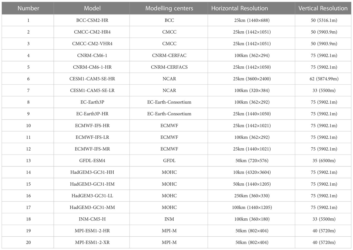
Table 2 Ensemble members of CMIP6 HighResMIP simulations used for the construction of background error covariance fields in the mapping scheme.
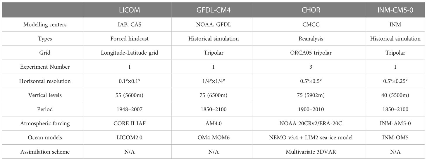
Table 3 Four members of models and ocean reanalyses used for the construction of background error covariance fields in the mapping scheme.
A localization strategy was also used in this mapping method, which assumes that only data within a specified length scale (defined by the influence radius) can propagate the signals during the analysis of a grid point. The fraction coverage of the mapping method was used to indicate the fraction of total ocean area that can be constrained by observations. The size of this area was defined by the influencing radius or spatial correlation length scales. This application helps to reduce the impact of the imperfect error covariance (i.e., the spurious remote correlations). Here we adopted a larger influence radius (R = 26°) from the sea surface down to 2000 m to obtain a near-global fractional coverage (more than 90%) for analysis (not shown here). Using this larger influence radius helps to utilize the remote spatial covariances and it helps to achieve a near-global fractional coverage for analysis and minimize a reconstruction bias in data-sparse regions due to the drift towards the prior guess (Durack et al., 2014; Cheng et al., 2017; Stammer et al., 2019; Cheng et al., 2020). However, the use of a large influence radius will lead to a smoothed spatial pattern by filtering out the smaller-scale signals. Following previous mapping methods (Cheng et al., 2020), the use of multi-step iterative scans shows a significant improvement in re-inserting the ocean variability across those spatial scales. Therefore, three iterative scans were performed using radii of 26°, 8°, and 4°. Other key parameters in this method can be found in the definitions in the study of Cheng et al. (2020).
To evaluate the performance of our reconstructed salinity results, a “subsample test” based on Argo-period observations (since 2007) was used in this study. Such a method has been validated in previous temperature/salinity reconstructions, including the impact of a localization strategy and the uncertainty due to the mapping method (Cheng and Zhu, 2016; Cheng et al., 2017; Cheng et al., 2020). We remark here that this procedure tested the impact of the changing sampling and climate state, it does not test the impact of the changes in the covariance function over time which requires further studies. In a subsample test, the observed salinity fields every six months from January 2007 to July 2017 were defined as the “truth” field (named “truth-obs”, total 22). For each “truth-obs”, the data within -2 to 2 months centered on each selected month were averaged to construct each “truth-obs” field to increase the data coverage. We subsampled each “truth-obs” as defined above, using different historical observation masks, selected every 60 months from January 1960 to January 2015 (so 12 observation masks are tested). Then all the subsampled fields (total 12×22, i.e., sampling 22 truth with 12 observation masks) were reconstructed by the mapping method and compare with the corresponding “truth-obs”. Here we defined their differences as the “sampling errors” to quantify the performance of the reconstruction.
Besides the Argo-period observations, synthetic observations were used to evaluate the mapping performance. The synthetic data were re-sampled from a high-resolution (0.25°×0.25° horizontally) CNRM-CM6-1-HR model in CMIP6 archive by the National Centre for Meteorological Research, Météo-France, and CNRS laboratory, and spans from 2007 to 2018 (historical simulation before 2015 and SSP2-4.5 after 2015) (Voldoire et al., 2019). The model simulations were regarded as “truth” field (named “truth-model” hereafter), which has global coverage and are dynamically consistent. We adopted 22 “truth-model” fields selected January and August from 2005 to 2015 and then we re-sampled them according to the observation locations on every 60 months from January 1960 to January 2015 (12 subsampled fields for each “truth-model” field, which are synthetic observations). There are a total of N=22×12 synthetic observation fields. Both IAP-1 and IAP-0.5 mapping methods were tested using this synthetic data approach and they have been averaged into 1° and 0.5° version, respectively.
2.2 Other salinity products
Five observational gridded products were used in this study for the comparison of multiscale salinity variability (Table S1): (1) EN4 from the UK Met Office (Gouretski and Reseghetti, 2010; Good et al., 2013); (2) Ishii from Japan (Ishii et al., 2017); (3) NCEI from the United States (Levitus et al., 2012); (4) IAP-1 from China (Cheng et al., 2020); (5) one Argo-based gridded monthly analysis, SCRIPPS from the United States (Roemmich and Gilson, 2009). Two additional ocean reanalysis data were included: (1) ORAS4 from the ECMWF (Balmaseda et al., 2013); (2) SODA from NOAA, USA (Carton et al., 2018). Among these products, SODA has the same horizontal resolution as the IAP-05 data, and the others have 1°×1° horizontal resolution. All the available products are converted into the same horizontal resolution and vertical depth levels as the new dataset for comparison. The climatology was constructed by the 12-month salinity data for the 1990–2010 period for the observations and model, which are used for mapping method to fill the data gaps. The salinity anomaly fields were then obtained by removing their own monthly climatology average before the analyses. Anomaly fields are compared in this study because of the following reasons: (1) It is a common practice to use anomalies to investigate variability and trend, so anomalies are much more relevant for climate variability and change researches; (2) In all previous studies, the mapping procedure is applied to the anomaly field rather than the absolute field because the anomalies are used to minimize the aliasing of the large spatial gradients of the climatological and seasonal fields into the mapping as a result of the sparse spatial resolution; (3) The procedure for constructing the absolute field (i.e. climatology) is always different from the mapping for anomalies, and their error sources and structure are different. Therefore, the climatology of each dataset should be removed to reduce the error related to climatology construction. The time span for each product is more than 55 years since 1960, with the exception of SODA, for which we used the 1980–2017 period.
To assess the quality of the new dataset, independent observations were also used. (1) The historical hydrographic observations in the Labrador Sea provided by the Bedford Institute of Oceanography (BIO) (Yashayaev, 2007). This hydrographic dataset includes the independently validated and bias-corrected multi-section surveys (i.e., AR7W) and profiles in the Labrador Sea, which span from 1896 to present. The physical parameters and transient anthropogenic traces from this dataset have been used to investigate the structures, properties, and impacts of Labrador Sea water, and some studies of the climate dynamics and change in the subpolar North Atlantic (Yashayaev and Loder, 2017). (2) The monthly SSS gridded version 3 product from the European Space Agency (ESA) Sea Surface Salinity Climate Change Initiative (CCI) consortium (Boutin et al., 2021). This dataset provides the improved calibrated global SSS fields with a 25km horizontal resolution of near-global coverage spanning from 2010 to 2019 based on the long-term multi-sensor salinity Climate Data Record, such as the SMOS (2010 to present), Aquarius (2011-2015) and SMAP (2015 to present) L-band radiometers. Consequently, it has the capacity to monitor the global SSS features, including its mesoscale variability and covers a longer period. (3) the gridded sea surface salinity dataset for the Atlantic Ocean, named LEGOS, which spans from 1980 to 2016 (Reverdin et al., 2007). The LEGOS data are based on the available data collected from 1970 to 2016 mostly from Voluntary Observing Ships, PIRATA moorings and Argo profiles and subsequently validated. This monthly SSS products is mapped by the objective analyzed method and covers the region between 95°W –20°E and 50°N–30°S in the Atlantic Ocean. Here we employed these observational datasets to test the ability of the IAP-05 dataset to capture small-scale and regional signals, and estimate of long-term linear trends.
3 Results
3.1 Evaluation based on the subsample test
3.1.1 Examples of the subsample test
The spatial pattern of the 50 m depth salinity anomalies on January 2017, the subsampled fields (for observation location of Januarys of 1960, 1990 and 2010 separately) and the reconstruction fields are presented in Figure 1. This subsample test uses the Argo-period observations. The ocean salinity field in January 2017 manifested as a dissipated La Ninãa-like pattern, with freshening in the tropical North Pacific and the Intertropical Convergence Zone (ITCZ), together with a salinity increase in the central and eastern Pacific. The northwest and southwest Pacific also experienced a significant salinity increase. The patterns of the reconstructed fields (Figure 1B) agree well with the “truth-obs” field for 2017, with a high spatial correlation coefficient of 0.61. The global-mean RMSD of the sampling errors for 2017 is 0.08, which is smaller than the reconstructed signals in most part of the global ocean. A good resemblance can be also found in the results of other subsample tests with a sparse historical distribution (Figures 1B, F, H). This consistency can also be found in their zonal patterns and the results for other periods (i.e., 1970, 1980 and 2000), with the positive salinity anomalies within 20°N–40°N,10°S–0° and 55°N–60°N, and negative values within 5°N–15°N and 20°S–10°S (Figure 1J). They provide indication that the new mapping method can reconstruct the “truth-obs” field given the sparse data distribution even back to 1960.
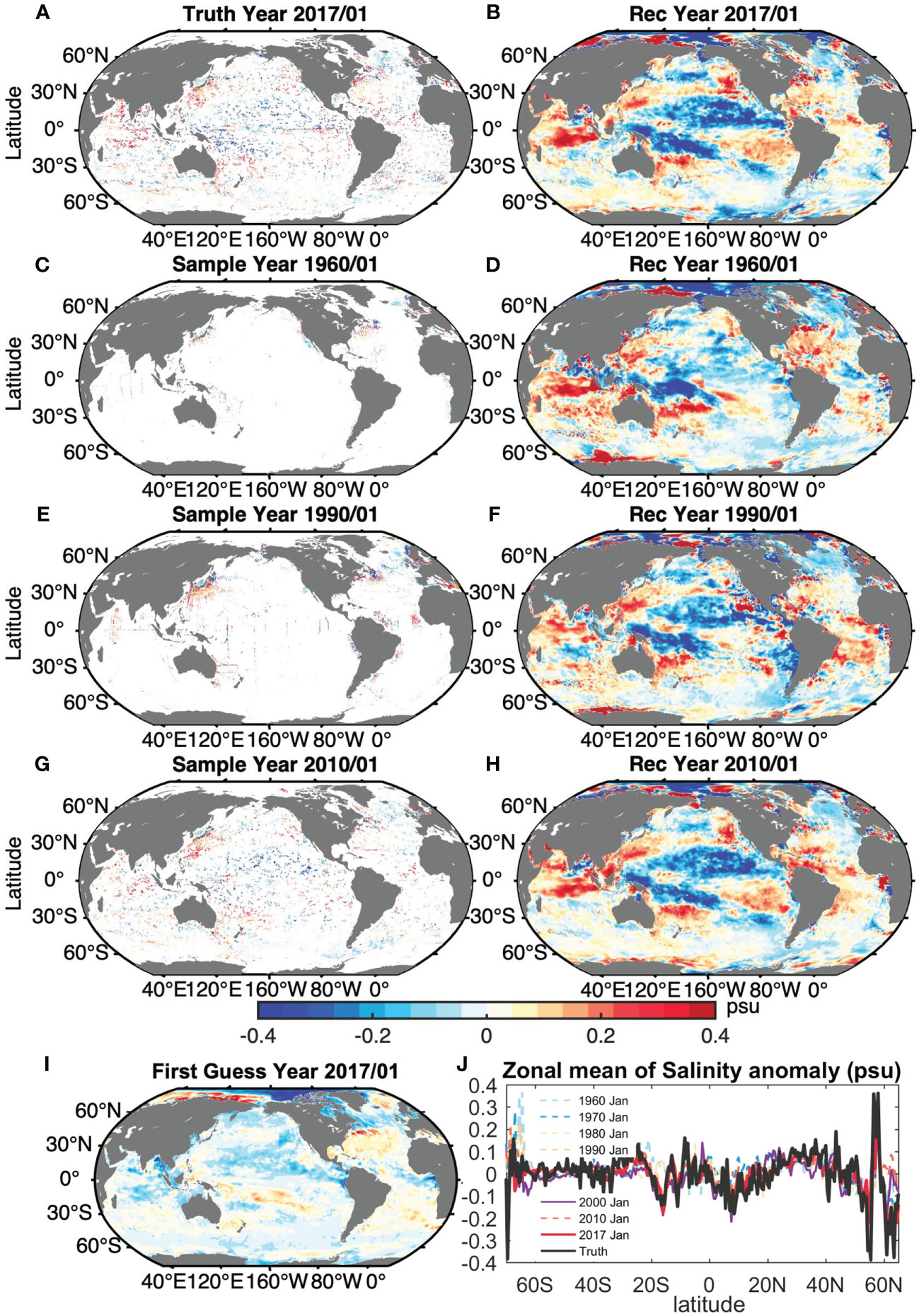
Figure 1 Reconstruction of historical salinity anomaly fields at 50 m depth (units: psu). (A–H) shows the truth field of salinity anomaly at 50 m in January 2017 and their subsampled fields according to the location of observations in Januarys of 1960, 1990 and 2010 (left panels). The reconstructed fields are shown in the right panels. (I) is the first guess field, and (J) is the reconstructed global zonal mean salinity anomaly along with the truth field (black line). The truth fields are based on the Argo-period observations in January 2017. The grid number of in situ observations in Januarys of 1960, 1970, 1980, 1990, 2000, 2010, 2017 are 2660, 5942, 6722, 8167, 5590, 15563 and 20397 for the 720×360 grid boxes.
In addition, it is apparent that the reconstruction field is very different from the first guess field, which is provided by the mean of ensemble members (used as a prior), even in the data sparse region such as the southern oceans (Figures 1B vs. 1I). To further quantify the potential impact of the first guess field, we manually replaced the first-guess field in IAP-05 mapping scheme with the climatology (zero anomaly), and then compared the reconstructed field with the previous reconstructed results, taking the 50m-depth salinity anomaly in January 1960 as an example (Figure S2). Both reconstructed fields show a consistent pattern (Figures S2B, S2D) and their difference also has a much smaller magnitude than the reconstructed results (Figure S2E). This test confirms that the first guess does play a minor role in our reconstruction, mainly because of the strong constraint of observations with the current mapping technique.
However, there are still some differences between the reconstructed field and the “truth-obs”, particularly before the Argo Period (i.e., 1960 and 1990), such as in the Southeast Pacific, South of Australia, and the southern subtropical Atlantic (Figure 1), indicating the uncertainty in reconstruction, which will be quantified by “subsample test” in the next section.
3.1.2 Subsample test using Argo-period data
The basin means of the salinity anomalies averaged over 0–2000 m (named S2000 hereafter) from 1960 to 2020 are shown in Figure 2, along with the corresponding mean sampling errors and sampling uncertainties. The global mean S2000 change (Figure 2A) shows a good resemblance to the IAP-1 result, decreasing with a rate of 0.005 ± 0.006 psu per century over the period 1960–2020 (The error range represents the 95% confidence interval of linear trends based on the ordinary least squares (OLS) linear fit). The Pacific Ocean experiences a robust freshening (−0.016 ± 0.004 psu per century) during 1960–2020, and the Atlantic Ocean yields a dramatic increase of 0.024 ± 0.013 psu per century since 1960. This shows that the new dataset can capture the increasing salinity contrast between the Atlantic and Pacific oceans (Curry et al., 2003; Durack et al., 2012). In the Indian Ocean, the S2000 change shows a strong decadal fluctuation, but with a slightly larger salinity value than the IAP-1 results before the 1980s. The S2000 for the IAP-05 and IAP-1 data show consistent decadal variation and a long-term decreasing trend (−0.008 ± 0.007 psu per century) of S2000 in the Southern Ocean. The reconstructed S2000 change in the Atlantic Ocean reveals a slightly positive systematic bias, while all other basins have negative systematic bias. The bias indicates the errors in the mapping method, likely rising from the bias in the error covariance given by models. Future improvement will be made if more and better high-resolution models are included to better estimate covariance. However, a systematic bias means an error in the mean state, and it has a small impact on the decadal and multi-decadal variabilities because the negative/positive bias is consistent over time within the uncertainty range. Moreover, the uncertainty in sampling error (2 standard deviations) reduced significantly after 2005 compared with before 2005, particularly in the Indian and Southern oceans. This reveals that the sampling uncertainty was decreasing with the increasing number of salinity observations.
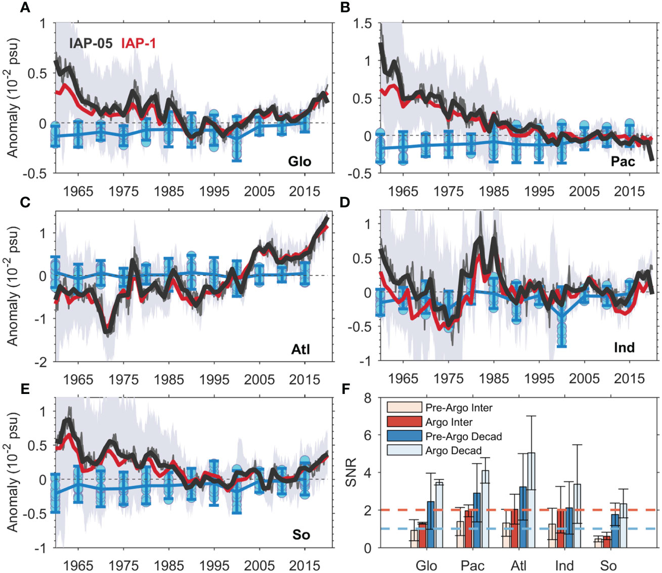
Figure 2 Global and basin means of the 0–2000 m salinity anomaly with sampling uncertainty. (A) Global (Glo), (B) Pacific (Pac), (C) Atlantic (Atl), (D) Indian (Ind), and (E) Southern oceans (So) (units: psu). The black line is the time series of the yearly mean of the salinity anomaly for IAP-05 and the red line is for the IAP-1 data. The grey line shows the monthly mean anomaly time series with the shading corresponding to two standard deviations of the ensemble members from the mean. The blue dots represent the sampling errors corresponding to 22 different truth fields based on the Argo-period observations, with the ensemble mean shown by the blue line and the vertical bars corresponding to two standard deviations. (F) The “signal over noise” ratio (SNR) for two different timescales: decadal/multidecadal (>7 years) and interannual (<7 years) for the pre-Argo (before 2005) and Argo (since 2005) periods.
To quantify the impact of sampling on the reconstructed interannual variability (smaller than 7 years) and decadal/multidecadal variability (greater than 7 years), we define the “signal over noise” ratio (SNR), calculated as the standard deviation (1σ) of the salinity time series divided by 1σ of the sampling error given in Figure 2. A 7-year high-pass filter was applied to the entire 1960–2020 time series to extract the interannual variation, and the 7-year low-pass filter was applied to obtain the interdecadal/multidecadal variation during the 1960-2020 period, consistent with Cheng et al. (2017); Cheng et al. (2020). Figure 2F shows the SNR for the decadal/multidecadal and interannual signals in different basins, separated into two different periods: the Pre-Argo period and the Argo period.
These interannual variations are smaller than or close to the sampling uncertainty (SNR ≤ 1) for almost all basins, especially for the Pre-Argo period, suggesting that the reconstructed interannual signals are more affected by the sampling uncertainty and then less reliable. For the decadal/multidecadal timescale, the SNR in all the basins is larger than 1, particularly in the Pacific, Atlantic and Indian oceans (SNR > 2). Since 2005, the reconstructed decadal variations in all the basins are significantly larger than the sampling uncertainty (SNR > 2). This suggests a more reliable reconstruction of decadal/multidecadal salinity variability in the recent decades, thanks to the establishment of Argo network. Meanwhile, for both time scales, the SNR during the Argo period is larger than that before 2005, suggesting a better reconstruction.
3.1.3 Subsample test using synthetic observations
Here we used the synthetic data to test IAP-1 and IAP-0.5 mapping performance. Figure 3 shows their vertical structures of global-mean salinity changes since 1960. Both versions showed consistent long-term changes of salinity, with significant freshening trends at sea subsurface (200~1200 m) and salinification trends at upper 200m (Figures 3A, B). To quantify the reconstruction performance, Figures 3C–F compares the reconstruction with the “truth-model” and shows the sampling error and its standard deviation for IAP-05 and IAP-1 respectively. The mean sampling errors for both IAP datasets are much smaller than the salinity anomalies (Figures 3C vs. A, D vs. B), indicating a reliable reconstruction by both approaches. IAP-1 mapping results in an overall positive bias (0~1200 m) and a negative bias below 1200m (Figure 3D), For the IAP-05 mapping, there is a small negative sampling error above 400m and a positive bias within 400–1600m before 2005. Since 2005, the negative bias extends down to 1000m and the positive error confines to depths 1000–1800m (Figure 3C). Besides, IAP-05 also shows smaller standard deviation than the IAP-1 data for all depths (Figures 3E vs. 3F). Figure S3 further shows the 0–2000m mean sampling errors for the global ocean and four major basins. In all the basins, the global and basin means of salinity errors for both mapping methods are smaller than the actual salinity change (Figure 2). By contrast, the mean sampling errors for the IAP-05 mapping method are smaller than that for IAP-1 method.
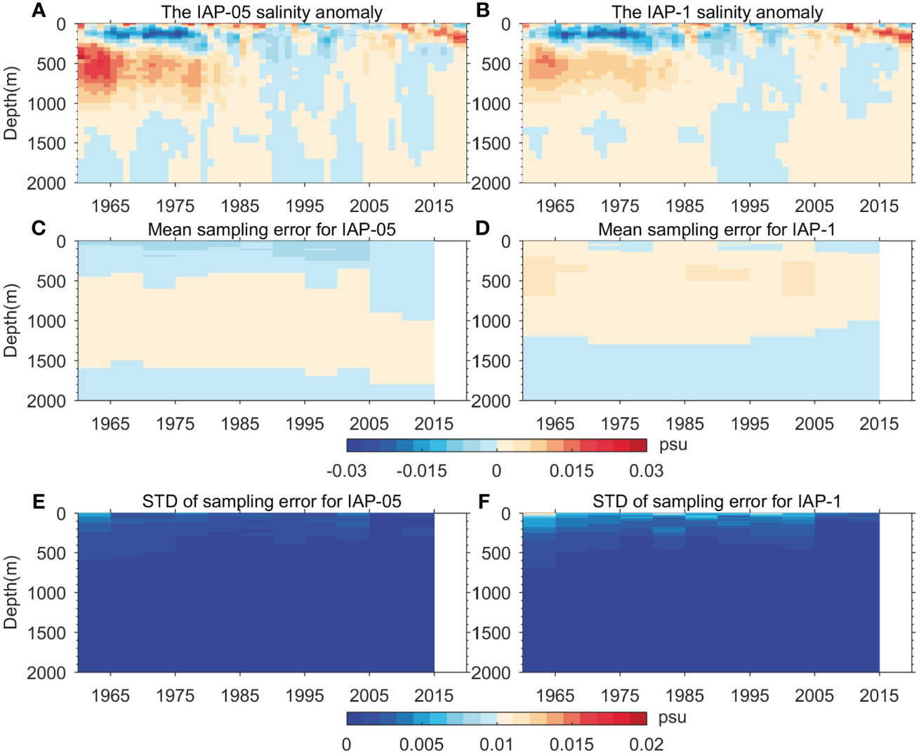
Figure 3 The reconstructed global-mean ocean salinity anomaly variations over depth from surface to 2000m (units: psu) for (A) IAP-05 and (B) IAP-1 data. (C) and (D) are their mean sampling errors for IAP-05 and IAP-1 data based on the “synthetic” subsample test, respectively, and (E) and (F) show their standard deviation of sampling errors.
The geographical distributions for the linear trends of the 0-2000 mean sampling errors and the globally zonal mean sampling errors of both IAP mapping methods based on the synthetic data are presented in Figure S4. Both IAP schemes display a similar pattern of change in sampling errors over time, and the magnitude of trend errors for the IAP-05 mapping method is generally smaller than IAP-1. For IAP-05, there are the negative biases appeared in the tropical and subtropical South Pacific Ocean, and the positive biases in West Atlantic Ocean. We note that the large sampling errors of both IAP salinity datasets occur in the Southern Ocean and their vertical distributions of negative anomalies correspond with the subduction pathway from the high latitudes (Figures S4C, S4D). Nevertheless, the sampling errors for both reconstructions are smaller than the actual salinity change signals (comparing Figure S4 of this study with Figure 6 in Cheng et al., 2020), indicating the robustness of the identified salinity trend patterns. Figure S5 further shows the distributions of standard deviation of linear trends of the sampling errors for both mappings, indicating a large uncertainty of trends reconstruction in the Boundary Current regions and subtropical gyres (Figures S5A, S5B) in the upper-200m ocean (Figures S5C, S5D). Compared with the IAP-1 results, the IAP-05 scheme shows a smaller and shallower uncertainty, which is mainly located in the boundary current regions in Southern hemisphere.
These results based on synthetic data with known “truth” suggest a better performance of the IAP-05 mapping method than the IAP-1 in illustrating the basin-scale salinity changes over the past decades.
3.2 Comparison with CCI satellite-based product
Here we provided additional assessments of the IAP-05 data by comparing the new dataset with the independent and high-resolution satellite gridded salinity product. As one goal of the IAP-05 is to provide a higher horizontal resolution dataset than IAP-1, CCI v3 gridded data at 25km horizontal resolution help us to testify its capacity to reveal the small-scale signals of the ocean. The mean SSS fields from January 2017 to December 2017 for CCI, IAP-05, and IAP-1 are shown in the Figure 4. For a fair comparison, both IAP salinity datasets were interpolated into the same horizontal resolution with CCI salinity product. All these products can reproduce the large-scale salinity characteristics, with a salinity maximum in the mid-latitudes, which is dominated by evaporation, and low values in the precipitation-dominated regions (i.e., the tropical and North Pacific) (Figures 4A, C, E). Both IAP datasets have the high spatial correlation coefficients of more than 0.97 with CCI data. Moreover, IAP-05 shows more details of mesoscale and small-scale spatial salinity distributions than the IAP-1 products.
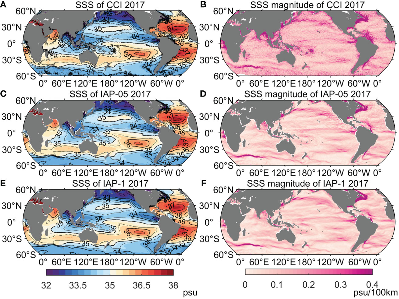
Figure 4 SSS (left panels, units: psu) and its horizontal gradient magnitude field averaged from January 2017 to December 2017 (right panels, units: psu/100 km) based on different products: (A, B) for CCI, (C, D) for IAP-05, and (E, F) for IAP-1. The SSS fields of IAP-05 and IAP-1 have been interpolated into the same horizontal resolution as the CCI data.
The magnitude of the horizontal gradients of SSS was also calculated in Figure 4 by the square root of the sum of squared zonal gradient and meridional gradient of SSS averaged from January 2017 to December 2017, following the method adopted in Vinogradova et al. (2019). This metric can illustrate the fine structure of the spatial variability of salinity. All the three products show similar salinity gradient patterns, including the stronger variability in the coastal and boundary currents regions, upwelling zones, and large-scale circulation convergence zones. The new IAP-0.5 dataset shows better consistency with CCI than IAP-1, such as the strong salinity fronts in the North Pacific Ocean, North Indian Ocean and Kuroshio extension regions.
Figure 5 shows the spatial maps of the mean difference and RMSD of SSS between both IAP datasets and CCI v3 satellite data from 2010 to 2019. Compared with CCI, IAP-05 and IAP-1 datasets have the global mean difference of –0.012 psu and –0.013 psu, respectively, and they show a consistent large-scale pattern with the positive differences in the tropical and subpolar regions in Pacific and Atlantic oceans, Bay of Bengal, Subtropical South Indian Ocean, and with the negative differences in the subtropical Pacific and Atlantic oceans, Arabian Sea and Southern oceans (South of 30°S), corresponding to the evaporation and precipitation dominated regions. We note that the magnitude of SSS signals for IAP-05 data are slightly smaller than the IAP-1 results. The largest values (>0.3 psu) are located in some coastal regions, such as the north of 45°N in the North Atlantic, and Antarctic Circumpolar Current (ACC) regions, where the large errors were present in CCI satellite data. Albeit for this difference, the spatial patterns of RMSD for both IAP datasets (Figures 4B, D) are consistent with the higher salinity values (>0.3 psu) in ITCZ regions, ACC regions in Indian Ocean, Kuroshio Current and its extension. They correspond to the largest mean difference for IAP products in these regions. The large RMSD for IAP-05 and IAP-1 (>0.4 psu) are also located in the coastal regions, where the CCI data have a larger uncertainty.
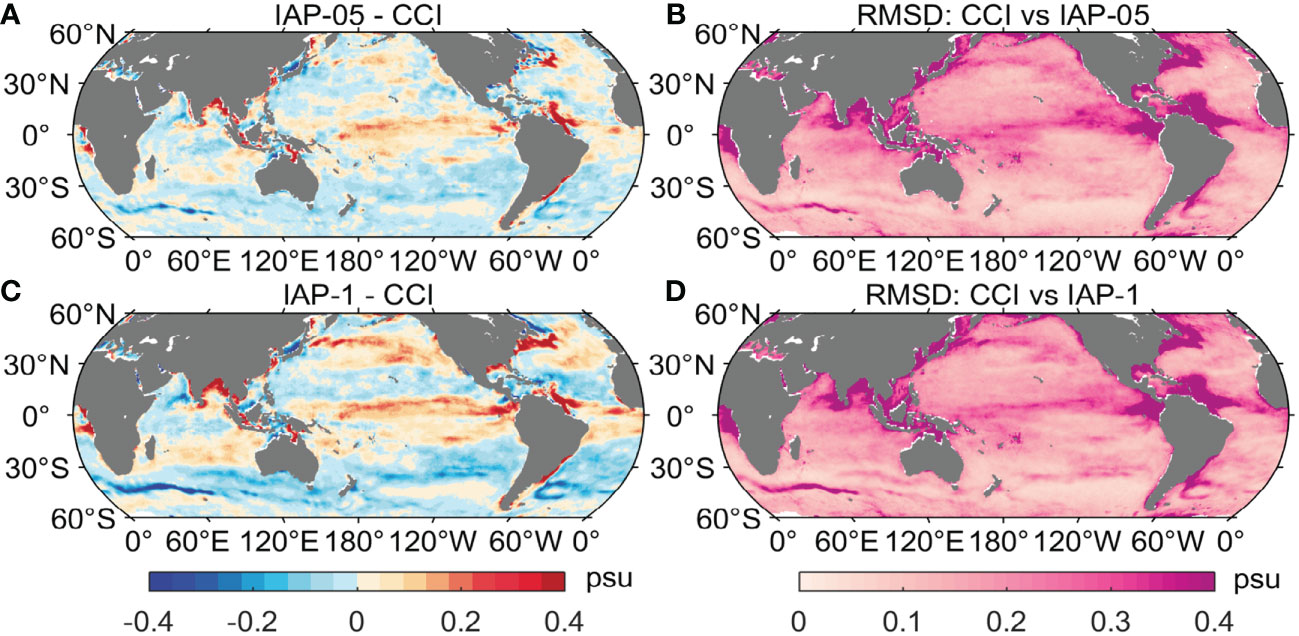
Figure 5 Mean difference (left panels) between (A) the IAP-05 and CCI SSS, (C) IAP-1 and CCI SSS during the 2010–2019 period. Root-mean-square deviation (RMSD, right panels) of the SMAP SSS with (B) IAP-05 SSS and (D) IAP-1 SSS during the 1990–2010 period. The SSS fields of IAP-05 and IAP-1 have been interpolated into the same horizontal resolution as the CCI data.
In summary, by comparing with an independent high-resolution satellite data, we show that the new IAP-05 data can better produce the smaller-scale signals than the 1° results.
3.3 Comparisons with other available observations
The subsample test and assessments using the independent satellite observations show that the 0.5° salinity field reconstructed using the proposed mapping method is a better representation of the salinity than 1° salinity field. In this section, we further compare the new dataset with other available gridded salinity datasets, in order to evaluate how well the current datasets could present the historical salinity variations on various spatial and time scales.
3.3.1 Salinity snapshots in the boundary and coastal regions
The increase in resolution should provide a better representation of some regional features that are not recognized in the 1° gridded resolution data, particularly in the western boundary and coastline regions. The 10 m depth salinity anomalies of the Kuroshio Current and its extension in January 2015 are shown in Figure 6 (this month is selected arbitrarily, using other time yields similar results). The IAP-05, IAP-1, EN4, Ishii, SCRIPPS, and both reanalyses (i.e., ORAS4 and SODA) are included for comparison. For a fair comparison, the 1° gridded datasets (i.e., IAP-1, EN4, Ishii, SCRIPPS and ORAS4) were interpolated into the horizontal resolution of 0.5°. As indicated in Figure 6, all the datasets can capture the large-scale characteristics of the salinity distribution in regions such as the zonal band of positive anomalies in the south of 20°N for the northwest Pacific. The patterns of EN4, Ishii and IAP-1 are smoother, while SCRIPPS and ORAS4 are able to show a few small-scale and mesoscale salinity signals. Compared with the 0.5° interpolated dataset, the high-resolution (including IAP-05 and SODA) results show a better representation of the salinity anomaly distribution in this selected region than other products in Figure 6. IAP-0.5 shows meandering features in the Kuroshio extension, which are more physically reasonable than other data such as IAP-1, EN4, and Ishii. Besides, the small-scale features in IAP-0.5 data are more consistent with in situ observations (Figures 6A vs. 6B).
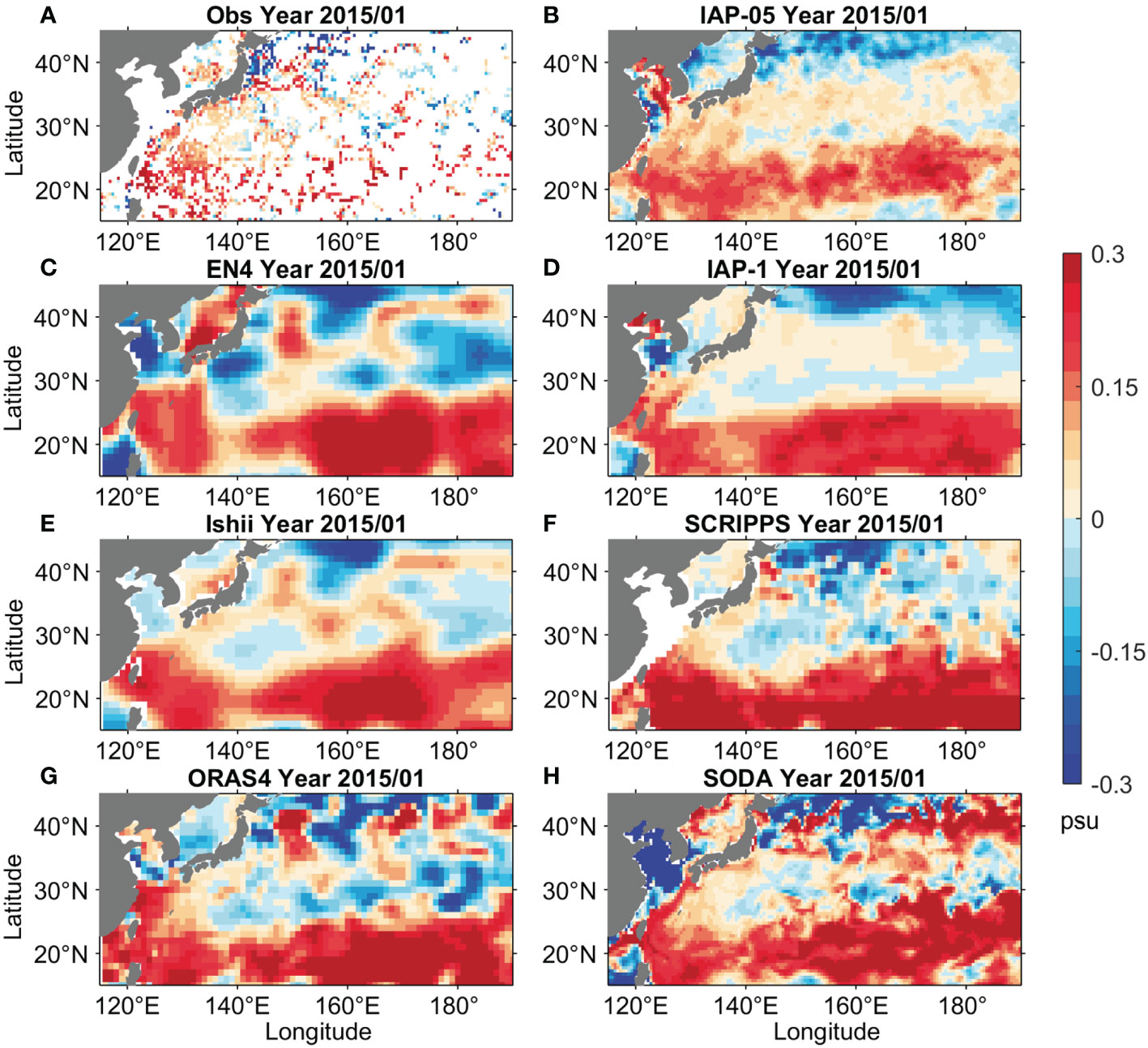
Figure 6 Comparison of 10m depth salinity anomaly (January 2015) in the Kuroshio Current and its extension for different gridded products. (A) Observations, (B) IAP-05, (C) EN4, (D) IAP-1, (E) Ishii, (F) SCRIPPS, (G) ORAS4, and (H) SODA (units: psu). The 1° gridded IAP-1, EN4, Ishii, SCRIPPS and ORAS4 have been interpolated into 0.5° versions.
Figure 6 shows that another improvement of the IAP-05 is the physical description of the coastline. This is because the 0.5° grid box is closer to the land and more confined to the coast than the 1° grid box (Locarnini et al., 2018). In particular, as SCRIPPS is based only on Argo observations, it shows no signal in some nearshore regions due to the absence of Argo data in shallow waters, such as the Bohai Sea, the Yellow Sea, East China Sea. This comparison suggests that higher resolution mapping could more effectively use the large amount of data near the coastal regions and in the boundary current regions.
3.3.2 Comparison with in situ observations
Here we compare different datasets with in situ salinity observations, based on the anomaly fields computed by removing the climatology over the 1990–2010 period. The in situ salinity data are the 0.5° gridded averaged fields without application of any spatial interpolation, which is used to reduce the sub-grid variability and to compensate the irregular spatial sampling. Figure 7 shows the 0–2000m averaged salinity anomalies differences between the gridded in situ data for the 1980-2017 period. The differences in coastal regions and regions where the depth is less than 2000m are estimated by using the salinity anomalies averaged to the local bottom. The small values in mean difference and RMSD for the new data with in situ gridded data could be expected because the observational sources of IAP-05 data are based on the in situ gridded data. IAP-05, IAP-1 and Ishii show a smaller magnitude of differences compared with the EN4 and two reanalysis products. The global average mean difference for IAP-05 is 0.003 psu; this value is smaller than that of other products. Both EN4 and SODA show the largest global average mean difference (0.007 psu). The largest salinity differences for all salinity datasets are located in some coastal regions and high-latitude areas, such as the big differences in East China Sea, subpolar North Atlantic, equatorial West Atlantic, and ACC region, revealing the impacts of large salinity variability. IAP-05 data shows notably smaller biases in the West Pacific, Intertropical Convergence Zone (ITCZ) and South Pacific Convergence Zone (SPCZ) regions than the other datasets. For EN4 and the two reanalyses, the positive biases of the salinity (>0.02 psu) are evident in the tropical Indian and southern Atlantic oceans, and the negative biases in the southeast Pacific and southern Indian oceans (<–0.02 psu).
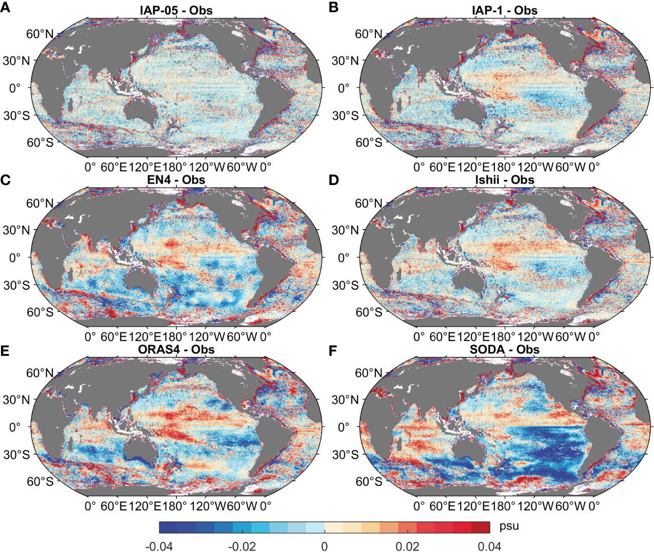
Figure 7 Mean differences of 0-2000m averaged salinity anomalies between (A) IAP-05, (B) IAP-1, (C) EN4, (D) Ishii, (E) ORAS4, (F) SODA and the gridded in situ data during 1980–2017. All the salinity climatology fields are relative to 1990–2010. The 1° gridded IAP-1, EN4, Ishii and ORAS4 have been interpolated into 0.5° versions.
Figure S6 illustrates the spatial distribution of the 0–2000m and 1980–2017 averaged RMSD of salinity products relative to the gridded in situ salinity data. All the datasets show the smaller RMSD (mostly <0.03 psu) in the tropical oceans and subtropical North Pacific than in other places. Large RMSD values (>0.05 psu) can be found in the Boundary current regions (i.e., Kuroshio Current and its extension) and some coastal areas, and the subtropical North Atlantic and ACC regions in Indian Ocean. IAP-05, IAP-1 and Ishii data have lower values of RMSD than EN4 and two reanalysis products in most places, with the global-mean RMSD of 0.057 psu for EN4, 0.059 psu for ORAS4 and 0.065 psu for SODA. The IAP-05 data show the smallest values of 0.045 for the global mean of RMSD, and the global-mean RMSD for IAP-1 is 0.052 psu. For the SODA, the largest RMSD (>0.05 psu) also appears in the Southeast Pacific, which is not found in other datasets.
Figure 8 further shows the global mean difference and RMSD of salinity anomalies compared with observations from surface to 2000m. All the datasets indicate the larger values of difference and RMSD in the near surface layer and they decrease with depth. The IAP-05 shows the smallest difference and RMSD in these gridded salinity products and its large values are found in the upper 50m with <0.01 psu for mean difference and <0.02 psu for RMSD. For other datasets, larger salty biases are found at the upper 200m. Among them, SODA shows the larger salty bias above 1000m and the largest RMSD in the 0–200m layer and 600–1000m reaching to more than 0.03.
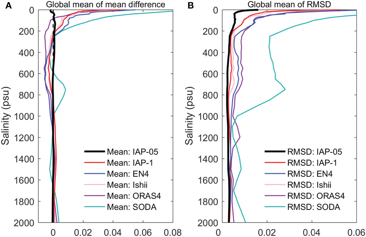
Figure 8 The vertical distribution of mean difference (A) and RMSD (B) of global-mean salinity anomalies over 2000m between the gridded in situ data and IAP-05, IAP-1, EN4, Ishii, ORAS4 and SODA during 1980–2017. All the salinity climatology fields are relative to 1990–2010. The 1° gridded IAP-1, EN4, Ishii and ORAS4 have been interpolated into 0.5° versions.
Figure S7 indicates the time variations of global mean difference of globally 0–2000m mean salinity anomalies during 1980–2020 compared with in situ observations. Although salt is conserved in the global ocean, it is expected that the mean salinity of the upper 2000 m is not constant and has the global mean freshening associated with the melting of land ice, and large decadal variations. Most products (except SODA) show the significant decrease of errors after 2005. ORAS4 shows a peak of salty bias over the 1995–2005 period. IAP-05 data shows the smallest values of mean difference over the whole period and IAP-1 also has the similar magnitude except within 1995–2000. SODA salinity data show an exceptional large positive bias before 1990 and a negative bias after 2005.
In summary, by comparing with in situ observations, we show that the new IAP-0.5 dataset has smaller mean difference and RMSD than the other products. However, we note that the in situ observations are processed by the authors’ group, thus the results in this section can’t be regarded as a fully independent and fair comparison between IAP-05 with other products. This is a caveat, but such comparison is still a useful addition to the tests provided in previous sections because all products are based on essentially the same in situ data from WOD.
3.3.3 Long-term trends of salinity
The long-term changes of SSS and subsurface salinity have been identified as indicators of the global-warming induced water cycle intensification, thus it is useful to compare different products for their representation of the long-term trends.
Figure 9 shows the spatial pattern of the salinity trends from 1980 to 2017 for all the gridded products. All ocean analyses (IAP-05, IAP-1, EN4, Ishii, NCEI) show a robust signature of the salinity pattern amplification, that is “the fresh gets fresher, and the salty gets saltier”, including the increased salinity contrast with the freshening (salinification) in Pacific (Atlantic) Ocean (Figures 9A–E). But there are major differences in magnitude and locations. Ishii data shows the weakest salinity increase in the subtropical Pacific and a much broader freshening in the tropical Pacific Ocean compared with other observational analyses (Figure 9D). The results of EN4 and NCEI (Figures 9C, E) show some patchy or spotty distributions (contours are isotropic), which is likely associated with the use of a parameterized covariance assuming Gaussian distribution (Boyer et al., 2005; Good et al., 2013).
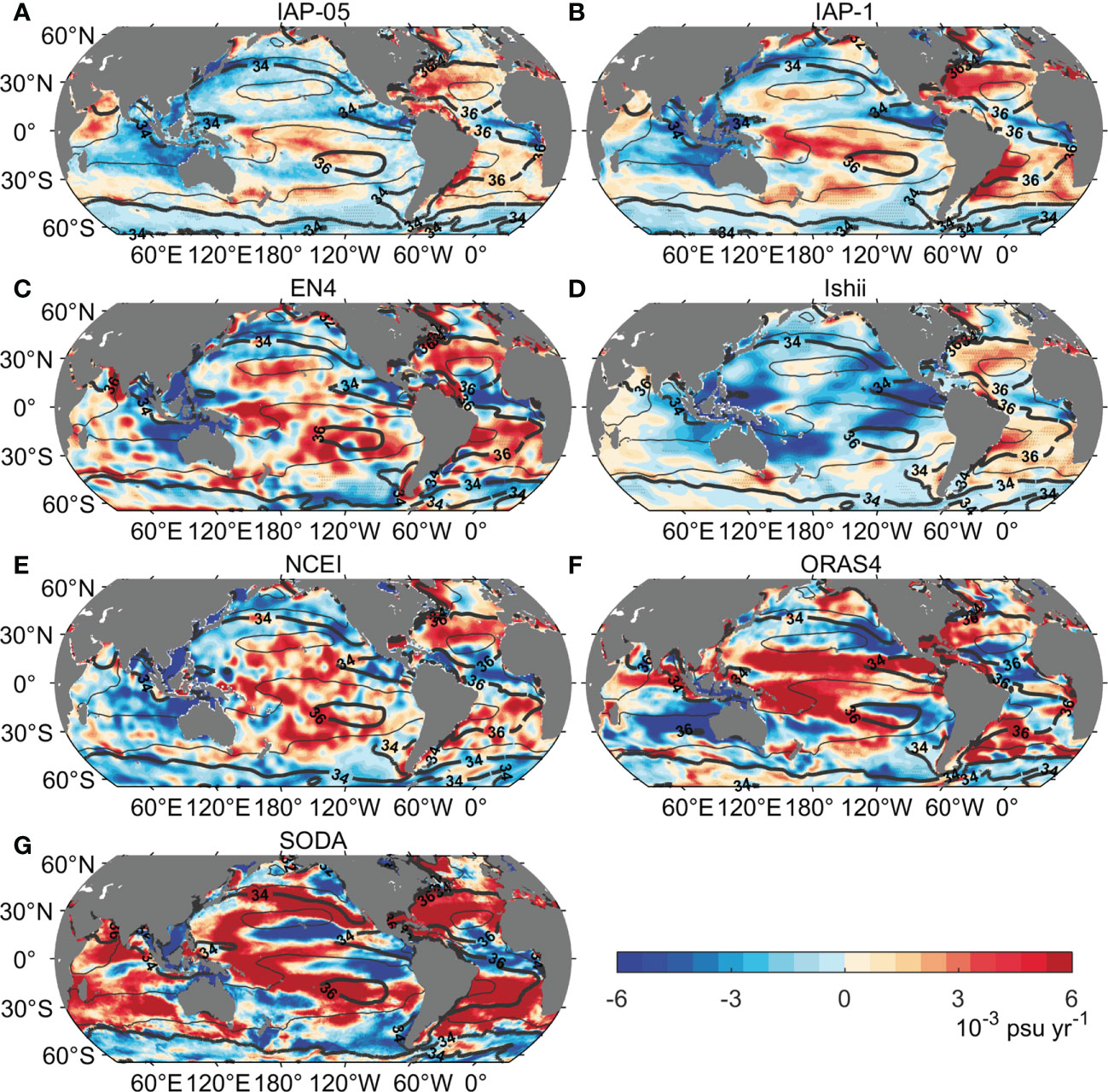
Figure 9 Spatial patterns of the sea surface salinity (SSS) long-term trends during the 1980–2017 period. (A) IAP-05, (B) IAP-1, (C) EN4, (D) Ishii, (E) NCEI, (F) ORAS4, and (G) SODA (units: 10−3 psu yr−1). Contour lines show the associated climatological mean salinity (1990–2010; units: psu). Linear trends are significant at the 95% confidence level in the dotted areas. The 1° gridded IAP-1, EN4, Ishii and ORAS4 have been interpolated into 0.5° versions.
The reanalyses (i.e., ORAS4 in Figure 9F and SODA in Figure 9G) show marked differences in trend’s magnitudes compared with the observational analyses (Figures 9A–E): their linear trends are much larger than the observational analyses in most places. Their spatial pattern correlations against the observational analyses are always smaller than 0.33 (Table 4). By contrast, the correlations between observational analyses are always >0.30 and even get to ~0.73 (between IAP-05 and IAP-1) (Table 4). Besides, for ORAS4, the signals of salinity increase in the subtropical Pacific are distributed more southward than the other products. And the inter-basin contrast of SSS trend between the Pacific (fresher) and Atlantic (salter) is smaller for ORAS4 and SODA than the other products (Figures 9F, G). These comparisons indicate a distinction between reanalyses (ORAS4 and SODA) and the observational datasets, which are probably impacted by the surface forcing, model biases and its assimilation scheme (Balmaseda et al., 2013; Carton et al., 2019).
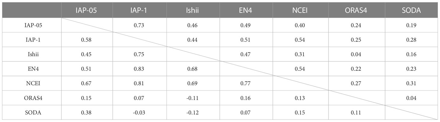
Table 4 The correlation of linear trends of global SSS (above diagonal) and globally zonal mean of subsurface salinity (below diagonal) between the 0.5-degree salinity data (all data are interpolated to 0.5°×0.5° resolution).
The new estimate of SSS trend is further compared with the LEGOS and other data in the tropical and subtropical Atlantic (30°S–50°N) during the period of 1980–2016 (Figure S8). All the datasets show are consistent for the large-scale patterns, showing the salinity increase in the subtropical North and South Atlantic and the freshening in the tropical Atlantic Ocean. The magnitude of trend in IAP-05 data is slightly weaker than the results for the IAP-1, EN4 and two reanalyses, but more consistent with Ishii and LEGOS. The Ishii also shows the weakest magnitude and SODA displays the largest SSS trends in the tropical and subtropical Atlantic. The spatial patterns are similar for all datasets, to quantify the similarity of the spatial pattern between LEGOS and different salinity products, here we calculated the spatial correlations. The highest correlation coefficient is 0.33 for LEGOS versus IAP-05, and Ishii data shows the smallest coefficient (~0.14), indicating LEGOS and IAP-05 are more consistent than LEGOS versus the other datasets. We note that the spatial correlation between IAP-05 and IAP-1 data is 0.55.
The long-term trends in the globally zonal mean subsurface salinity of these datasets also show an overall enhancement of the existing mean pattern (Figure 10), with the high correlation coefficients between two spatial fields for both datasets and even reaching to 0.83 (between IAP-1 and EN4) (Table 4). This is closely associated with a downward propagation of salinity anomalies into the ocean interior in recent decades, corresponding to a salinity increase of the salty subtropical waters and freshening of the high-latitude waters. Again, the spatial correlations between reanalyses (ORAS4 and SODA) and other observational datasets are low or even negative (i.e., –0.11 and 0.12 for ORAS4 and SODA vs Ishii suggesting major differences are in the subsurface ocean. The biggest differences between ORAS4 and other datasets are located around 40°N extending to depths of ~2000 m and ~30°S above 200 m (Figure 10F).
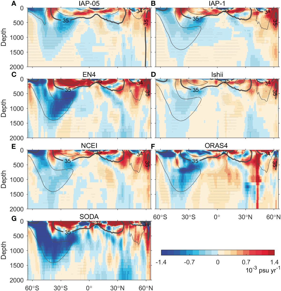
Figure 10 Spatial patterns of the long-term trends in globally zonal mean subsurface salinity (0–2000 m) during the 1980–2017 period. (A) IAP-05, (B) IAP-1, (C) EN4, (D) Ishii, (E) NCEI, (F) ORAS4, and (G) SODA (units: 10−3 psu yr−1). Contour lines show the associated climatological mean salinity (1990–2010, units: psu). Linear trends are statically significant at the 95% confidence level in the dotted areas. The 1° gridded IAP-1, EN4, Ishii and ORAS4 have been interpolated into 0.5° versions.
Given the distinction between reanalysis and analysis in our comparison, a thorough comparison among reanalysis products is urgently needed to better understand the uncertainty. A similar analysis has been done for ocean heat content (Palmer et al., 2017), showing much larger spread among ocean reanalyses than observational products. Similar results are expected for salinity as well, because the reanalysis products are subject to additional errors from the inaccurate ocean model (especially at subsurface), surface forcing, and assimilation scheme.
3.3.4 ENSO-related SSS variability in the Pacific Ocean
ENSO is a dominant mode of variability in the tropical Pacific (Qu and Yu, 2014; Zhi et al., 2019). The phase of ENSO is commonly indicated by the Ninão 3.4 index, which is defined as the three-month running mean of SST averaged in the region of 5°S–5°N, 170°W–120°W (Trenberth, 1997). To compare the capability of different products in demonstrating the ENSO-related SSS changes in the tropical Pacific, we regressed the SSS anomalies onto the Ninão3.4 index for each individual dataset during the Argo period (2005–2017) and the Pre-Argo period (1980-2004), respectively (Figure 11).
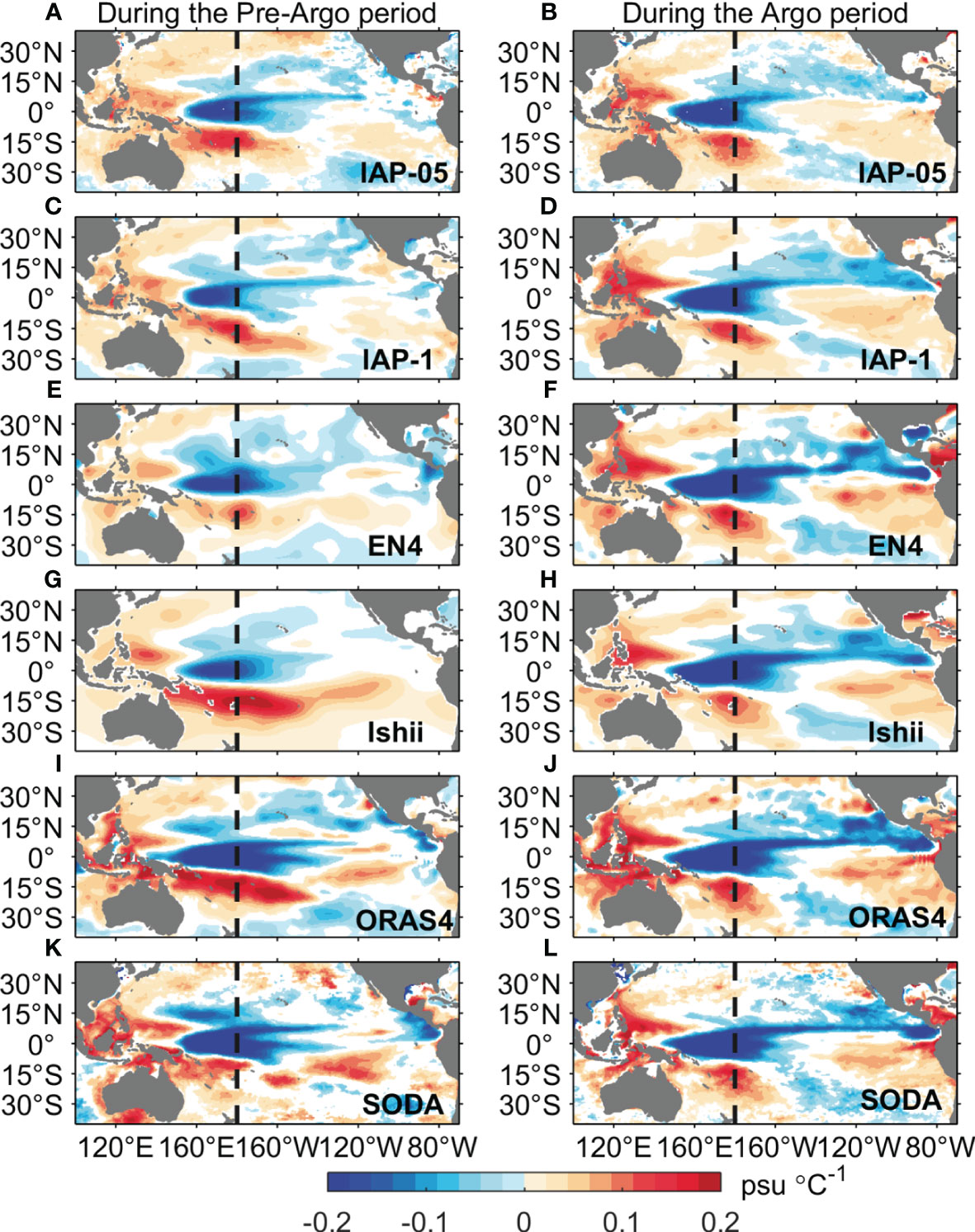
Figure 11 Linear regressions of the SSS (anomalies on the Niño 3.4 index during the Pre-Argo period (1980–2004, left panels) and during the Argo period (2005–2017, right panels) for different gridded products (units: psu °C−1). (A) and (B) for IAP-05, (C) and (D) for IAP-1, (E) and (F) for EN4, (G) and (H) for Ishii, (I) and (J) for ORAS4, and (K) and (L) for SODA. All variables are detrended and smoothed using a three-month running mean. The blank regions indicate that the regression coefficients are not statically significant at the 95% confidence level. Black dashed lines indicate the location of 180°E. The 1° gridded IAP-1, EN4, Ishii and ORAS4 have been interpolated into 0.5° versions.
All the regressed SSS patterns in our study are similar to those in previous studies (Roemmich and Gilson, 2011). During the El Ninão phase, the strongest negative SSS anomalies occur in the western-central equatorial Pacific, centered near 175°E and extending to the northeastern Pacific along the west coast of North America, which roughly coincides with the eastward displacement of the warm pool along the Equator. Three positive cores are also found near the Philippine coast, over the SPCZ, and in the southeastern tropical Pacific. However, a better consistency is found during the Argo period (right panels in Figure 11) than the Pre-Argo period (left panels in Figure 11), associated with the increasing data amount and data quality since 2005 (Riser et al., 2016). For the objective analysis products, the magnitude of the regressed anomalous SSS fields before the Argo period is weaker than that during the Argo period, particularly in the southeast Pacific (Figures 11A–H). The EN4 and Ishii data display some patchy and spotty distributions in the western and southeast Pacific, particularly before the Argo Period. While the ENSO patterns for IAP-05 and IAP-1 are more physically consistent than that for EN4 and Ishii during the Pre-Argo Period, because they are well constrained by observations, given the near-global fraction coverage (>90%) of their mapping methods. The positive anomalies in the SPCZ for the ORAS4 and Ishii data (Figures 11G, I) are much larger than the results from other datasets. The SODA reanalysis shows another negative anomaly pole in the tropical northern Pacific (>0.15 psu °C-1), and its magnitude is larger than other datasets (Figure 11K). Compared with other salinity products, the new dataset and IAP-1 seems to be more capable of depicting the ENSO-related SSS modes during these two periods.
3.3.5 S-IOD events
Strong salinity variations are also found in the tropical Indian Ocean (IO). Previous studies have shown that the meridional salinity dipole mode in the tropical Indian Ocean (S-IOD) is a predominant mode of SSS variability in the tropical IO (Zhang et al., 2016; Zhang et al., 2017). In its positive phase, there is a contrast with low (high) salinity anomalies in the southern equatorial (tropical southeastern) IO. The S-IOD shows multiple time-scale variabilities and is triggered by many processes, including the ocean advection driven by equatorial IO winds and the surface freshwater flux variability in the Southern tropical IO, the decadal modulation of the Indo-Pacific Walker circulation and Indonesian Throughflow (Zhang et al., 2017). Furthermore, the S-IOD index is used to represent the evolution of the S-IOD events, which is defined as the SSS anomaly (SSSa) difference between the southeastern IO (22°–12°S, 98°–118°E) and the central equatorial IO (8°S–2°N, 70°–90°E) (Zhang et al., 2016). Here, S-IOD index is calculated in each individual dataset, and then it is regressed onto the spatial SSS anomalies in the tropical IO for each dataset. The analysis is separated into two periods (2005–2017 and 1980–2004) to test the robustness of the results (Figures S9, S10).
The typical S-IOD mode of the significant meridional SSSa dipole during the Argo period is well indicated by all the salinity results (Figure S9), with contrasting low (high) SSS anomalies at its northern (southern) poles. With higher resolution, IAP-05 and SODA are able to provide a more detailed description of the salinity distribution. Before the Argo period, all the salinity products can capture the main characteristics of the S-IOD mode, but with some differences in the locations and magnitude (Figure S10). For example, compared with the regression results during the Argo period, the center of the positive SSS anomaly for EN4 is located farther north and east; the scope of the positive salinity anomalies for the Ishii data is stronger but located farther east; and IAP-05 shows a weaker southern pole but strong positive anomalies in West Indian Ocean (Figure S10A).
3.3.6 Interdecadal salinity change in the Subpolar North Atlantic
The Atlantic Meridional Overturning Circulation (AMOC) is the key component of world ocean’s thermohaline circulation, and its variation plays an important role in modulating the global climate variability (Rahmstorf et al., 2015; Lozier et al., 2019). As the primary ventilation region in the North Atlantic, the interdecadal variations in deep convection of the Labrador Sea is one of major issues for AMOC research.
The hydrographic datasets for the Labrador Sea have accumulated a large number of historical salinity profiles (they are not included in WOD) and thus can be considered as an independent data for the validation of our new dataset and other products. On the basis of these hydrographic observations, Figure 12 shows the time series of the mean salinity anomaly averaged over 200–2000 m in the Central Labrador Sea since 1960. The salinity change in this layer acts as a regulator of the density in the Labrador Sea with the significant interdecadal variability, corresponding to the concurrent deep convection process and variation in AMOC strength (Yashayaev and Loder, 2016). The salinity decreased from the early 1970s, picked up in the early 1990s, and then began to decrease again during 2012–2013. In 2011, the salinity anomaly returned to a relatively strong positive value, but smaller than its peak value in the early 1970s. This may be attributed to the impact of global warming on the salinity in this region and the AMOC (Collins et al., 2013).
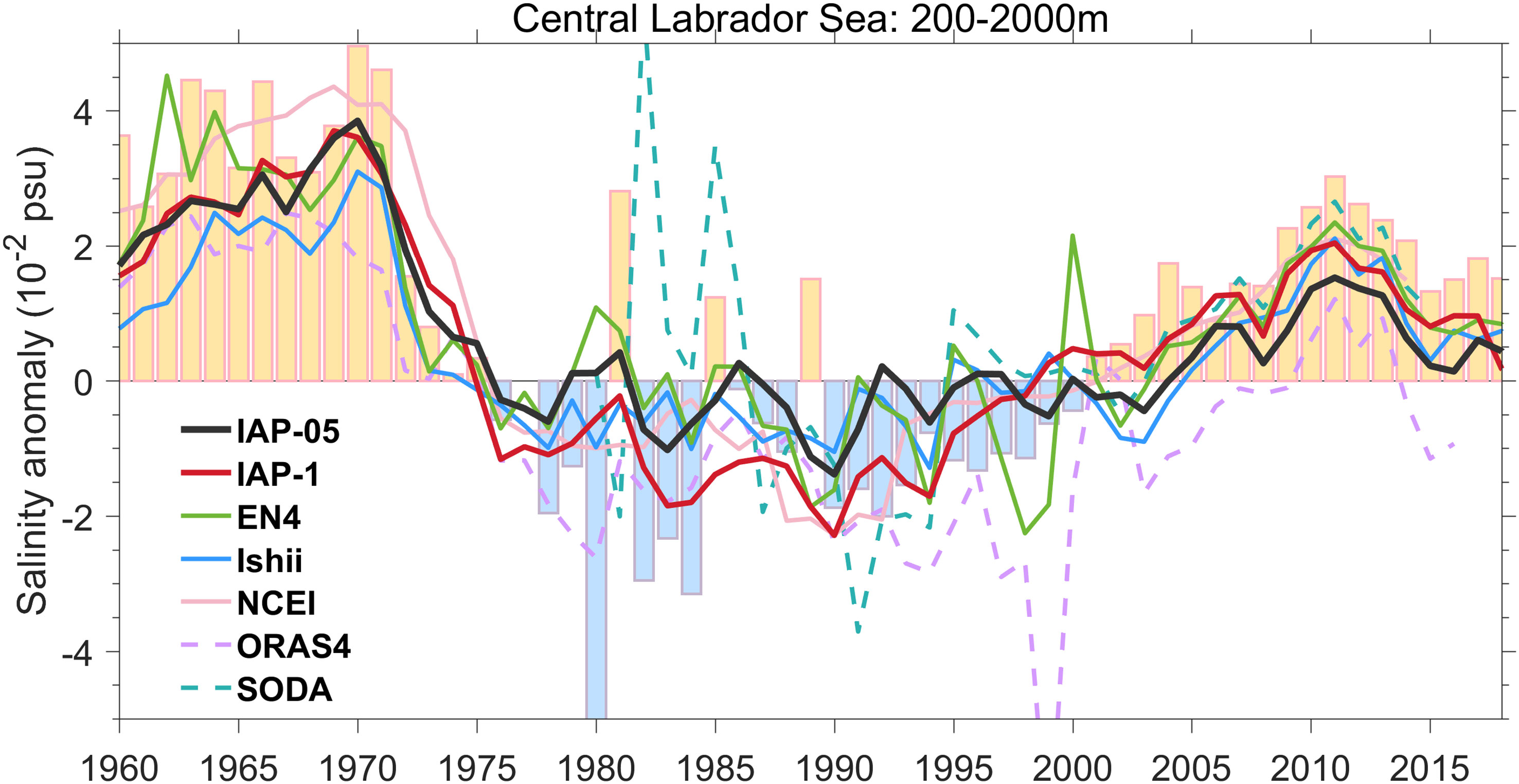
Figure 12 Mean salinity anomaly changes averaged over 200–2000m in the central Labrador Sea (units: 10−2 psu). The vertical bars correspond to the individual observations and the different colored lines represent different salinity products.
For the salinity products, SODA can capture the change in phase since the 1990s, but it had some spikes within 1982–1987 that are stronger than the magnitude of the positive peak in the early 1970s. ORAS4 also had some spikes in the time series around 1999, and did not return to the positive phase after 2005. All the datasets could capture the positive peak during the period of 1960s and 1970s, and Ishii and ORAS4 show the relatively smaller magnitude. Since then, the IAP-05, NCEI, EN4, and Ishii data show relatively weaker negative salinity anomalies during the 1980–2000 period. After 2005, all the salinity products tended to be consistent, except for the ORAS4, and IAP-05 shows a slightly weaker positive anomalies than other datasets. The salinity variation of IAP-1 data agrees better with the independent observations than the IAP-05 results, and it has the highest correlation of ~0.81 with that of observations, despite the high correlation of ~0.75 for IAP-05.
4 Discussions
Few salinity observations are available spatially or temporally, leaving numerous data gaps. Several salinity analysis and reanalysis datasets have been implemented based on different reconstruction schemes and sources of observations in recent decades. This study introduced a new IAP salinity gridded dataset with a horizontal resolution of 0.5° from surface to 2000m since 1960. We first describe the mapping framework of IAP-05 and evaluate its performance. This new dataset is built from a new ENOI-DE scheme of dynamic ensembles, which are derived from the ensemble members of high-resolution models and ocean reanalyses. The evaluation of IAP-05 performance includes the subsample test based on the Argo observations and Synthetic data; comparisons with in situ observations, high-resolution satellite-based product, gridded SSS dataset for the Atlantic Ocean and independent observations in Labrador Sea. Collectively, our evaluation results indicate that the proposed method can better reconstruct the historical salinity changes than IAP-1 product and can better represent the ocean salinity structure.
A comparison of the salinity multiscale variabilities and patterns between the IAP-05 and several salinity gridded datasets is also presented, including ocean analyses (i.e., IAP-1, EN4, Ishii, SCRIPPS and NCEI) and reanalyses (i.e., ORAS4 and SODA). We focused on the following main aspects: (1) the spatial patterns in the western boundary regions and near the coastline; (2) the long-term mean state and linear trends of SSS and the global zonal mean subsurface salinity; (3) the ENSO-related salinity variability in the tropical Pacific Ocean; (4) the S-IOD variability in the tropical Indian Ocean; (5) the decadal salinity variation in the subpolar North Atlantic. The results are summarized below.
The comparison of salinity anomalies with in situ data in the western boundary regions demonstrates the advantage of high-resolution version. It provides a better representation of salinity anomaly features, particularly in the mesoscale and small scale, and near the boundary current systems and coastal regions. Besides, the dataset allows more effective use of observations near the coastal regions and in the boundary current regions. For the long-term trends of surface and subsurface salinity, the ocean analyses can represent an amplification of the existing salinity mean state, while ORAS4 and SODA reanalyses show much larger spread. The ENSO-related salinity patterns and S-IOD associated patterns show a good consistency among multiple products, albeit with some differences in locations and magnitude, and time periods. Both IAP datasets indicate better consistency with the hydrographic datasets in illustrating the interdecadal salinity variation in subpolar North Atlantic. However, this study only provides an inter-comparison among products, regional differences and their relationship with controlling factors (i.e., rainfall change and ocean advection) need to be further investigated, for example, by analyzing specific ENSO and S-IOD events.
The comparison of the gridded salinity datasets is useful for understanding climate changes at different temporal and spatial scales, and the improvement of data reconstruction. The differences among products provide reference points for the application of salinity gridded datasets. In the future, an important step is to understand the source of error in salinity datasets, including data quality control, vertical interpolation method, mapping method, choice of climatology, data bias etc. The reanalysis also has additional errors from the inaccuracy of ocean model, surface forcing and assimilation scheme. Therefore, a comprehensive comparison and further analysis on the available analysis and reanalysis datasets are recommended, as a start to uncover the uncertainty in these datasets.
We acknowledge that our mapping method has some caveats. For example, the proposed method in this study can be impacted by the performance of the high-resolution model simulations because they provide covariance and first-guess estimate. Improvements and updates of models will feed back to the reconstruction of the historical subsurface salinity field in the future. The care also needs to be taken when using IAP salinity data for model evaluation and for detection and attribution studies. Furthermore, merging the SSS fields derived from recent and future satellites (i.e., Aquarius, SMOS and SMAP) into the in situ observation products will also be useful to better estimate the four-dimensional salinity state.
Data availability statement
The new dataset produced in this study and IAP-1 data are available at http://www.ocean.iap.ac.cn/. Other collected salinity data are as follows: NCEI (https://www.ncei.noaa.gov/access/global-ocean-heat-content/anomaly_data_s.html), EN4 (https://www.metoffice.gov.uk/hadobs/en4/download-en4-2-1.html), Ishii (https://climate.mri-jma.go.jp/pub/ocean/ts/v7.2/), SCRIPPS (https://argo.ucsd.edu/data/argo-data-products/), ORAS4 (http://apdrc.soest.hawaii.edu/datadoc/ecmwf_oras4.php), SODA (https://www2.atmos.umd.edu/~ocean/index_files/soda3.4.2_mn_download_b.htm). The outputs of CMIP5 models, GFDL-CM4, INM-CM5-0, and CMIP6 HighresMIP simulations are downloaded from the Earth System Grid Federation (ESFG; https://esgf-node.llnl.gov/projects/esgf-llnl/). CMCC Historical Ocean Reanalysis (CHOR) are available from http://c-glors.cmcc.it/index/index-9.html?sec=0), LICOM2.0 output is provided by State Key laboratory of numerical modeling for atmospheric sciences and geophysical fluid dynamics (LASG), Institute of atmospheric physics. CCI v3 salinity product is available from https://climate.esa.int/en/odp/#/project/sea-surface-salinity. LEGOS data is obtained from https://www.legos.omp.eu/sss/data-delivery/research-products/. The original contributions presented in the study are included in the article/Supplementary Material. Further inquiries can be directed to the corresponding authors.
Author contributions
GL drafted the manuscript and performed all the data analyses. LC proposed the main ideas and supervised all processes. YP contributed to the figure generation and data analysis. GW provided the high-resolution synthetic data and contributed to the subsample test. All authors contributed to the interpretation of results and the preparation of the manuscript. All authors contributed to the article and approved the submitted version.
Funding
This study is supported by the National Key R&D Program of China (Grant No. 2017YFA0603202), the Strategic Priority Research Program of the Chinese Academy of Sciences (Grant No. XDB42040402), National Natural Science Foundation of China (Grant No. 42122046, Grant No. 42076202, Grant No. 42206208) and Young Talent Support Project of Guangzhou Association for Science and Technology.
Conflict of interest
The authors declare that the research was conducted in the absence of any commercial or financial relationships that could be construed as a potential conflict of interest.
Publisher’s note
All claims expressed in this article are solely those of the authors and do not necessarily represent those of their affiliated organizations, or those of the publisher, the editors and the reviewers. Any product that may be evaluated in this article, or claim that may be made by its manufacturer, is not guaranteed or endorsed by the publisher.
Supplementary material
The Supplementary Material for this article can be found online at: https://www.frontiersin.org/articles/10.3389/fmars.2023.1108919/full#supplementary-material
References
Abraham J. P., Baringer M., Bindoff N. L., Boyer T., Cheng L. J., Church J. A., et al. (2013). A review of global ocean temperature observations: Implications for ocean heat content estimates and climate change. Rev. Geophysics 51, 450–483. doi: 10.1002/rog.20022
Balmaseda M. A., Mogensen K., Weaver A. T. (2013). Evaluation of the ECMWF ocean reanalysis system ORAS4. Q. J. R. Meteorol. Soc. 139, 1132–1161. doi: 10.1002/qj.2063
Boutin J., Reul N., Koehler J., Martin A., Catany R., Guimbard S., et al. (2021). Satellite-based Sea surface salinity designed for ocean and climate studies. J. Geophys. Res.: Oceans 126, e2021JC017676. doi: 10.1029/2021JC017676
Boyer T., Domingues C. M., Good S. A., Johnson G. C., Lyman J. M., Ishii M., et al. (2016). Sensitivity of global upper-ocean heat content estimates to mapping methods, XBT bias corrections, and baseline climatologies. J. Climate 29, 4817–4842. doi: 10.1175/JCLI-D-15-0801.1
Boyer T. P., Levitus S., Antonov J. I., Locarnini R. A., Garcia H. E. (2005). Linear trends in salinity for the world Ocean 1955–1998. Geophys. Res. Lett. 32, 67–106. doi: 10.1029/2004GL021791
Carton J. A., Chepurin G. A., Chen L. (2018). SODA3: A new ocean climate reanalysis. J. Climate 31, 6967–6983. doi: 10.1175/JCLI-D-18-0149.1
Carton J. A., Penny S. G., Kalnay E. (2019). Temperature and salinity variability in the SODA3, ECCO4r3, and ORAS5 ocean reanalyse 1993–2015. J. Climate 32, 2277–2293. doi: 10.1175/JCLI-D-18-0605.1
Cheng L., Trenberth K. E., Fasullo J., Boyer T., Abraham J., Zhu J. (2017). Improved estimates of ocean heat content from 1960 to 2015. Sci. Adv. 3, e1601545. doi: 10.1126/sciadv.1601545
Cheng L., Trenberth K. E., Gruber N., Abraham J. P., Fasullo J. T., Li G., et al. (2020). Improved estimates of changes in upper ocean salinity and the hydrological cycle. J. Climate 33, 10357–10381. doi: 10.1175/JCLI-D-20-0366.1
Cheng L., Zhu J. (2016). Benefits of CMIP5 multimodel ensemble in reconstructing historical ocean subsurface temperature variations. J. Climate 29, 5393–5416. doi: 10.1175/JCLI-D-15-0730.1
Collins M., Knutti R., Arblaster J., Dufresne J.-L., Fichefet T., Friedlingstein P., et al. (2013). Long-term Climate Change: Projections, Commitments and Irreversibility. In: INTERGOVERNMENTAL PANEL ON CLIMATE, C (ed.) Climate Change 2013 – The Physical Science Basis: Working Group I Contribution to the Fifth Assessment Report of the Intergovernmental Panel on Climate Change. Cambridge: Cambridge University Press.
Curry R., Dickson B., Yashayaev I. (2003). A change in the freshwater balance of the Atlantic ocean over the past four decades. Nature 426, 826. doi: 10.1038/nature02206
Durack P. J. (2015). Ocean salinity and the global water cycle. Oceanogr. 28, 20–31. doi: 10.5670/oceanog.2015.03
Durack P. J., Gleckler P. J., Landerer F. W., Taylor K. E. (2014). Quantifying underestimates of long-term upper-ocean warming. Nat. Clim. Change 4, 999. doi: 10.1038/nclimate2389
Durack P. J., Wijffels S. E. (2010). Fifty-year trends in global ocean salinities and their relationship to broad-scale warming. J. Climate 23, 4342–4362. doi: 10.1175/2010JCLI3377.1
Durack P. J., Wijffels S. E., Matear R. J. (2012). Ocean salinities reveal strong global water cycle intensification during 1950 to 2000. Science 336, 455. doi: 10.1126/science.1212222
Garcia H. E., Boyer T. P., Locarnini R. A., Baranova O. K., Zweng M. M. (2018). World ocean database 2018: User’s manual (prerelease). Ed. Mishonov A. V. (NOAA, Silver Spring, MD). Available at: https://www.NCEI.noaa.gov/OC5/WOD/pr_wod.html.
Good S. A., Martin M., Rayner N. A. (2013). EN4: Quality controlled ocean temperature and salinity profiles and monthly objective analyses with uncertainty estimates. J. Geophys. Res. 118, 6704–6716. doi: 10.1002/2013JC009067
Gouretski V., Reseghetti F. (2010). On depth and temperature biases in bathythermograph data: Development of a new correction scheme based on analysis of a global ocean database. Deep-sea Res. Part I-Oceanogr. Res. Pap. 57, 812–833. doi: 10.1016/j.dsr.2010.03.011
Greene C. H., Monger B. C., Mcgarry L. P., Connelly M. D., Schnepf N. R., Pershing A. J., et al. (2012). Recent Arctic climate change and its remote forcing of Northwest Atlantic shelf ecosystems. Oceanogr. 25, 208–213. doi: 10.5670/oceanog.2012.64
Haarsma R. J., Roberts M. J., Vidale P. L., Senior C. A., Bellucci A., Bao Q., et al. (2016). High resolution model intercomparison project (Highresmip V1.0) for CMIP6. Geosci. Model Dev. 9, 4185–4208.
Held I. M., Guo H., Adcroft A., Dunne J. P., Horowitz L. W., Krasting J., et al. (2019). Structure and performance of GFDL’s CM4.0 climate model. J. Adv. Modeling Earth Syst. 11, 3691–3727. doi: 10.1029/2019MS001829
Hosoda S., Ohira T., Nakamura T. (2008). A monthly mean dataset of global oceanic temperature and salinity derived from argo float observations. JAMSTEC Rep. Res. Dev. 8, 47–59. doi: 10.5918/jamstecr.8.47
Hosoda S., Suga T., Shikama N., Mizuno K. (2009). Global surface layer salinity change detected by argo and its implication for hydrological cycle intensification. J. Oceanogr. 65, 579. doi: 10.1007/s10872-009-0049-1
Ishii M., Fukuda Y., Hirahara S., Yasui S., Suzuki T., Sato K. (2017). Accuracy of global upper ocean heat content estimation expected from present observational data sets. SOLA 13, 163–167. doi: 10.2151/sola.2017-030
Jan D. Z., Nikolaos S., Adam T. B., Robert M., Nurser A. J. G., Josey S. A. (2018). Improved estimates of water cycle change from ocean salinity: the key role of ocean warming. Environ. Res. Lett. 13, 074036. doi: 10.1088/1748-9326/aace42
Katsura S., Ueno H., Mitsudera H., Kouketsu S. (2019). Spatial distribution and seasonality of halocline structures in the subarctic north pacific. J. Phys. Oceanogr. 50, 95–109. doi: 10.1175/JPO-D-19-0133.1
Levitus S., Antonov J. I., Boyer T. P., Baranova O. K., Garcia H. E., Locarnini R. A., et al. (2012). World ocean heat content and thermosteric sea level change (0–2000 m), 1955–2010. Geophys. Res. Lett. 39 (L10603), 1–5. doi: 10.1029/2012GL051106
Li L., Schmitt R. W., Ummenhofer C. C., Karnauskas K. B. (2016). Implications of north Atlantic Sea surface salinity for summer precipitation over the US Midwest: Mechanisms and predictive value. J. Climate 29, 3143–3159. doi: 10.1175/JCLI-D-15-0520.1
Li G., Zhang Y., Xiao J., Song X., Abraham J., Cheng L., et al. (2019). Examining the salinity change in the upper pacific ocean during the argo period. Clim. Dyn. 53, 6055–6074. doi: 10.1007/s00382-019-04912-z
Liu C., Liang X., Chambers D. P., Ponte R. M. (2020). Global patterns of spatial and temporal variability in salinity from multiple gridded argo products. J. Climate 33, 8751–8766. doi: 10.1175/JCLI-D-20-0053.1
Locarnini M., Mishonov A., Baranova O., Boyer T., Zweng M., Garcia H., et al. (2018). World Ocean Atlas 2018, Volume 1: Temperature, NOAA Atlas NESDIS 81, 52.
Lozier M. S., Li F., Bacon S., Bahr F., Bower A. S., Cunningham S. A., et al. (2019). A sea change in our view of overturning in the subpolar north Atlantic. Science 363, 516. doi: 10.1126/science.aau6592
Lu S., Li H., Xu J., Liu Z., Wu X., Sun C., et al. (2018). Manual of global ocean argo gridded data set (BOA_Argo) (Version 2018). Available at: https://argo.ucsd.edu/wp-content/uploads/sites/361/2020/07/User_Manual_BOA_Argo-2020.pdf.
Palmer M. D., Roberts C. D., Balmaseda M., Chang Y. S., Chepurin G., Ferry N., et al. (2017). Ocean heat content variability and change in an ensemble of ocean reanalyses. Clim. Dyn. 49, 909–930. doi: 10.1007/s00382-015-2801-0
Qiu B., Chen S. (2012). Concurrent decadal mesoscale eddy modulations in the Western north pacific subtropical gyre. J. Phys. Oceanogr. 43, 344–358. doi: 10.1175/JPO-D-12-0133.1
Qu T., Yu J.-Y. (2014). ENSO indices from sea surface salinity observed by aquarius and argo. J. Oceanogr. 70, 367–375.
Rahmstorf S., Box J. E., Feulner G., Mann M. E., Robinson A., Rutherford S., et al. (2015). Exceptional twentieth-century slowdown in Atlantic ocean overturning circulation. Nat. Clim. Change 5, 475–480. doi: 10.1038/nclimate2554
Reverdin G., Kestenare E., Frankignoul C., Delcroix T. (2007). Surface salinity in the Atlantic ocean (30°S–50°N). Prog. Oceanogr. 73, 311–340. doi: 10.1016/j.pocean.2006.11.004
Rhein M., Rintoul S. R., Aoki S., Campos E., Chambers D., Feely R. A., et al. (2013). Observations: Ocean in climate change 2013: The physical science basis. Ed. Stocker T. F., et al (Cambridge and New York: Cambridge University Press).
Riser S. C., Freeland H. J., Roemmich D., Wijffels S. E., Troisi A., Belbeoch M., et al. (2016). Fifteen years of ocean observations with the global argo array. Nat. Clim. Change 6, 145–153. doi: 10.1038/nclimate2872
Roberts M. J., Jackson L. C., Roberts C. D., Meccia V., Docquier D., Koenigk T., et al. (2020). Sensitivity of the atlantic meridional overturning circulation to model resolution in CMIP6 HighResMIP simulations and implications for future changes. J. Adv. Model. Earth Syst. 12, E2019ms002014.
Roemmich D., Gilson J. (2009). The 2004–2008 mean and annual cycle of temperature, salinity, and steric height in the global ocean from the argo program. Prog. Oceanogr. 82, 81–100. doi: 10.1016/j.pocean.2009.03.004
Roemmich D., Gilson J. (2011). The global ocean imprint of ENSO. Geophys. Res. Lett. 38, L13606. doi: 10.1029/2011GL047992
Roemmich D., Johnson G. C., Riser S. C., Davis R. E., Gilson J., Owens W. B., et al. (2009). The argo program: observing the global ocean with profiling floats. Oceanogr. 22, 34–43. doi: 10.5670/oceanog.2009.36
Ross E., Behringer D. (2019). Changes in temperature, pH, and salinity affect the sheltering responses of Caribbean spiny lobsters to chemosensory cues. Sci. Rep. 9, 1–11. doi: 10.1038/s41598-019-40832-y
Skliris N., Marsh R., Josey S. A., Good S. A., Liu C., Allan R. P. (2014). Salinity changes in the world ocean since 1950 in relation to changing surface freshwater fluxes. Clim. Dyn. 43, 709–736. doi: 10.1007/s00382-014-2131-7
Stammer D., Bracco A., Achutarao K., Beal L., Bindoff N. L., Braconnot P., et al. (2019). Ocean climate observing requirements in support of climate research and climate information. Front. Mar. Sci. 6. doi: 10.3389/fmars.2019.00444
Taylor K. E., Stouffer R. J., Meehl G. A. (2012). An overview of CMIP5 and the experiment design. Bull. Am. Meteorol. Soc. 93, 485–498. doi: 10.1175/BAMS-D-11-00094.1
Trenberth K. E. (1997). The definition of El niño. Bull. Am. Meteorol Soc. 78, 2771–2778. doi: 10.1175/1520-0477(1997)078<2771:TDOENO>2.0.CO;2
Vinogradova N., Lee T., Boutin J., Drushka K., Fournier S., Sabia R., et al. (2019). Satellite salinity observing system: Recent discoveries and the way forward. Front. Mar. Sci. 6. doi: 10.3389/fmars.2019.00243
Vinogradova N. T., Ponte R. M. (2017). In search of fingerprints of the recent intensification of the ocean water cycle. J. Climate 30, 5513–5528. doi: 10.1175/JCLI-D-16-0626.1
Voldoire A., Saint-Martin D., Sénési S., Decharme B., Alias A., Chevallier M., et al. (2019). Evaluation of CMIP6 deck experiments with Cnrm-Cm6-1. J. Adv. Model. Earth Syst. 11, 2177–2213.
Volodin E. M., Mortikov E. V., Kostrykin S. V., Galin V. Y., Lykosov V. N., Gritsun A. S., et al. (2017). Simulation of modern climate with the new version of the INM RAS climate model. Izv. - Atmos. Ocean. Phys. 53, 142–155.
Xue Y., Wen C., Kumar A., Balmaseda M., Fujii Y., Alves O., et al. (2017). A real-time ocean reanalyses intercomparison project in the context of tropical pacific observing system and ENSO monitoring. Clim. Dyn. 49, 3647–3672. doi: 10.1007/s00382-017-3535-y
Yan Y., Chassignet E. P., Qi Y., Dewar W. K. (2013). Freshening of subsurface waters in the Northwest pacific subtropical gyre: Observations and dynamics. J. Phys. Oceanogr. 43, 2733–2751. doi: 10.1175/JPO-D-13-03.1
Yang C., Masina S., Storto A. (2017). Historical ocean reanalyses, (1900–2010) using different data assimilation strategies. Q. J. R. Meteorol Soc. 143, 479–493. doi: 10.1002/qj.2936
Yashayaev I. (2007). Hydrographic changes in the Labrador Sea 1960–2005. Prog. Oceanogr. 73, 242–276. doi: 10.1016/j.pocean.2007.04.015
Yashayaev I., Loder J. W. (2016). Recurrent replenishment of Labrador Sea water and associated decadal-scale variability. J. Geophys. Research: Oceans 121, 8095–8114. doi: 10.1002/2016JC012046
Yashayaev I., Loder J. W. (2017). Further intensification of deep convection in the Labrador Sea in 2016. Geophys. Res. Lett. 44, 1429–1438. doi: 10.1002/2016GL071668
Yu Y., Liu H., Lin P. (2012). A quasi-global 1/10 eddy-resolving ocean general circulation model and its preliminary results. Chin. Sci. Bull. 57, 3908–3916. doi: 10.1007/s11434-012-5234-8
Zhang Y., Du Y., Ming F. (2017). Multi-time scale variability of the sea surface salinity dipole mode in the tropical Indian ocean. J. Climate 31, 283–296. doi: 10.1175/JCLI-D-17-0271.1
Zhang Y., Du Y., Qu T. (2016). A sea surface salinity dipole mode in the tropical Indian ocean. Clim. Dyn. 47, 2573–2585. doi: 10.1007/s00382-016-2984-z
Zheng F., Zhang R. (2015). Interannually varying salinity effects on ENSO in the tropical pacific: A diagnostic analysis from argo. Ocean Dyn. 65, 691–705. doi: 10.1007/s10236-015-0829-7
Zhi H., Zhang R.-H., Lin P., Yu P. (2019). Interannual salinity variability in the tropical pacific in CMIP5 simulations. Adv. Atmos. Sci. 36, 378–396. doi: 10.1007/s00376-018-7309-1
Keywords: Ocean salinity, mapping method, climate variability, observations, climate change
Citation: Li G, Cheng L, Pan Y, Wang G, Liu H, Zhu J, Zhang B, Ren H and Wang X (2023) A global gridded ocean salinity dataset with 0.5° horizontal resolution since 1960 for the upper 2000 m. Front. Mar. Sci. 10:1108919. doi: 10.3389/fmars.2023.1108919
Received: 26 November 2022; Accepted: 28 February 2023;
Published: 16 March 2023.
Edited by:
Sabrina Speich, École Normale Supérieure, FranceReviewed by:
Gilles Reverdin, Centre National de la Recherche Scientifique (CNRS), FranceJohn Church, University of New South Wales, Australia
Copyright © 2023 Li, Cheng, Pan, Wang, Liu, Zhu, Zhang, Ren and Wang. This is an open-access article distributed under the terms of the Creative Commons Attribution License (CC BY). The use, distribution or reproduction in other forums is permitted, provided the original author(s) and the copyright owner(s) are credited and that the original publication in this journal is cited, in accordance with accepted academic practice. No use, distribution or reproduction is permitted which does not comply with these terms.
*Correspondence: Lijing Cheng, Y2hlbmdsaWpAbWFpbC5pYXAuYWMuY24=