 Youk Greeve
 Per Bergström
 Åsa Strand
 Mats Lindegarth
94% of researchers rate our articles as excellent or good
Learn more about the work of our research integrity team to safeguard the quality of each article we publish.
Find out more
ORIGINAL RESEARCH article
Front. Mar. Sci., 24 January 2023
Sec. Marine Biology
Volume 10 - 2023 | https://doi.org/10.3389/fmars.2023.1105999
Introduction: As suspension-feeders, bivalves play a key role in maintaining regulatory functions of coastal ecosystems, which are linked to important ecosystem services. The functions attributed to bivalves depend on the life habits of a species (epi- or infauna) and their abundance and biomass. To properly quantify and assess these functions, detailed information the distribution, abundance and biomass at the ecosystem scale is critical. Amongst others, this requires an understanding on how environmental conditions shape special patterns in distribution. In this study we investigate this fundamental information on the Swedish west coast, an area where this information is lacking.
Methods: A survey which was designed to representatively sample both epi- and infaunal bivalves from randomized locations in various habitat types was conducted. Specifically, abundance and biomass of all species were recorded in the intertidal (0-0.5 m) and the shallow subtidal zone (0.5-2 m). The sites were distributed over an offshore gradient and at two exposure levels. This sampling structure allowed to extrapolate the results to an ecosystem level though information on the areal extent of these habitats using GIS layers.
Results: It was found that even though there exist a great variability among sites, in general epifaunal bivalves outweigh infaunal bivalves approximately 3 to 1. In terms of abundance, the ratio is more or less reversed and infaunal species occur in greater numbers. Most bivalves were found at an intermediate level of exposure, but due to the areal extend of the sheltered inner-archipelago this was the most important habitat for bivalve abundance and biomass. It was also found that invasive epifaunal oyster Magallana gigas and the invasive infaunal clam Ensis leei both dominated their respective groups in terms of biomass.
Discussion: Though the survey was relatively small, these results serve as a valuable insight of the relative importance of epi- and infaunal bivalves in this region. This gives understanding on which species and habitats are particularly important for ecosystem functions and services related to bivalves. This also provide a starting baseline for attempts to quantify ecosystem services provided by certain species or groups of bivalves in the future.
Coastal marine ecosystems are characterized by strong physical and chemical gradients which interact to create a large variety of benthic and pelagic environments that are key for habitat forming species and their associated communities. Complex interactions between these species further shape the physical, chemical and biological state of these coastal ecosystems (e.g. Sueiro et al., 2011; Velasco-Charpentier et al., 2021), altering important functions and processes (Meadows et al., 2012; Guy-Haim et al., 2018). Functions which are especially relevant in the coastal zone include benthic and pelagic primary production, which enhance the concentration of organic carbon into the system (Falkowski et al., 1998), secondary production and decomposition that contribute to nutrient cycling (Ramesh et al., 2015) and modification of benthic habitats by creating more structural complexity (Sueiro et al., 2011) and by reworking sediments (e.g. bioturbation and irrigation), which increases fluxes of oxygen in the sediment and facilitates resuspension (Aller, 1988; Norling et al., 2007).
Coastal ecosystems have had profound contributions to the organization and welfare of human societies. Historically the most obvious contributions include the provision of food (e.g. fish, shellfish, seabirds and mammals) and efficient routes for transport and trade (Martínez et al., 2007). However, increasing anthropogenic pressures such as climate change and competition for space and resources from a diverse set of sources and users are putting more and more coastal ecosystems and their functions at risk (Jackson et al., 2001; Harley et al., 2006; Lotze et al., 2006; Duarte et al., 2008; Cloern et al., 2016). The concept of ecosystem services was proposed to describe and quantify contributions of ecosystems towards the wellbeing of human society, which would lead to more effective policy making [Costanza et al., 1997; Bouma & Van Beukering, 2015; but see also the related concept “natures contribution to people” (Díaz et al., 2018)]. Identifying such services helps high-lighting not only the use values that can be values that can be traded on a market such as food provision, but also includes non-use values (e.g. cultural and regulatory services), which can rarely be traded but are still valuable or essential to people, societies and ecosystems (Gómez-Baggethun et al., 2010; Barbier et al., 2011). Better understanding of the contribution of these services to human welfare, and particularly the ecological processes and functions upon which they are based, is critical for efficient management of coastal areas including protection and restoration of valuable services (Forêt et al., 2018).
Bivalves are regarded as important components in many of the world’s coastal ecosystems (Dame, 2016). Through their ubiquity and ability to form dense assemblages, they can have multiple effects on the functions of ecosystems and typically contribute in multiple ways to the structure and services of ecosystems (Smaal et al., 2018). Firstly, by feeding on suspended particles they can affect the water column clarity (Peterson and Heck, 2001; Newell, 2004) and exert top-down control of phytoplankton communities (Prins et al., 1997; Riisgård et al., 2007; Grabowski et al., 2012). At the same time, nutrients are captured from the pelagic and transported to the benthos where they are further processed by bacterial communities, supporting important benthic-pelagic processes (Norkko et al., 2001; Kellogg et al., 2014; Ehrnsten et al., 2020). Furthermore, many bivalve species provide and modify habitat for other species, thus supporting the maintenance of biodiversity (e.g. Norkko et al., 2001; Norling and Kautsky, 2007; Humphries et al., 2011; Norling et al., 2015; McLeod et al., 2019) and sometimes have a stabilizing effect on coastal sediments by attenuating shear stress caused by waves and currents, thus mitigating coastal erosion (Wiberg et al., 2019). Finally, but not least important, harvesting or farming of bivalves provide valuable food, income and cultural values to human societies in most coastal areas of the world (van der Schatte Olivier et al., 2020). In many densely populated areas, however, human exploitation of wild bivalve populations has been extensive in recent history (MacKenzie et al., 1997). This has resulted in deterioration of many habitats, particularly those dominated by various types of oysters (Beck et al., 2011), which has led to a great reduction in their associated services (Coen et al., 2007; Grabowski et al., 2012; zu Ermgassen et al., 2013). Now, a greater appreciation and understanding for the ecological roles of bivalves exists, and a shift towards viewing bivalves as an integral component of coastal ecosystem function and health has occurred, from solely that of secondary producers and a source of nutrition. Among other things, this has resulted in numerous efforts to restore and maintain the associated services from bivalves, either through the restoration of natural populations or strategic aquaculture placement (Humphries et al., 2016; Bersoza Hernández et al., 2018).
The majority of bivalves can be categorized into two functional groups based on their position and mode of living in benthic habitats: epifaunal and infaunal species (Gosling, 2004). Infaunal bivalves are species that burrow either partially or completely in soft sediments. In contrast, epifaunal species live on top of the sea floor, generally attached to natural or artificial hard substrates and conspecifics. Despite the fact that most bivalve species are filter-feeders, it is important to note that the mode of living has fundamental consequences for how they interact with the environment and how they contribute to ecosystem services. For example, epifaunal bivalves typically provide structural complexity for other species and trap fine sediment within the shell matrix of their aggregations, hence support biodiversity (Norkko et al., 2006), organic enrichment of sediment and sediment stabilization (van der Zee et al., 2016; Christianen et al., 2017). Infaunal bivalves on the other hand, depending on the species, their densities and the environmental conditions, can either contribute to the bioturbation (i.e. erodability) and bioirrigation of the sediment (Norkko and Shumway, 2011), or can facilitate the build-up of organic matter (Bouma et al., 2009). Both processes affect the oxygenation and thus bacterial heterotrophic and chemolithotrophic activity within the sediment (Hansen et al., 1996; Newell et al., 2002), and thus contribute to the nutrient cycling processes.
Evidently, many ecological functions are to some degree species-specific and variable among functional groups, and the ecological importance of a species or a functional group will hence vary with their spatial distribution and abundance, both in terms of population density (e.g. habitat provision and modification) and biomass (e.g. filtration capacity) (Whitlatch et al., 1997; Beadman et al., 2004; Ciutat et al., 2007; Sandwell et al., 2009). Thus, to understand the role of different types of bivalves and the potential importance of various ecological processes, such as filtration, habitat modification and production, representative and quantitative data on the distribution of species and, importantly, overall representation, is critical.
Despite the ecological and economic importance of many bivalve species, quantitative information on the distribution and composition of bivalve species from Swedish coastal waters is surprisingly scarce and no targeted monitoring exists of the shallow subtidal and intertidal inhabited by the variety of bivalve species known to occur in the region. Information from these habitats comes mainly from qualitative surveys on the extent of mussel and oyster beds performed or commissioned by regional authorities (summarized in: (Lindegarth et al., 2014; in Swedish), or from occasional research studies, usually in a restricted area and focusing on one or a small number of species (e.g. Evans & Tallmark, 1977; Möller & Rosenberg, 1983; Lindegarth et al., 1995; Wrange et al., 2010; Bergström et al., 2021). With Evans and Tallmark (1977) being the only exemption, we are not aware of any studies assessing and comparing the abundance and biomass of epi- and infaunal species in this region. This lack of representative, synoptic data on all major bivalve ecosystem components represents an obstacle to the understanding of the quantitative importance of the bivalve community in coastal waters.
Therefore, the aim of this study was to quantify the distribution and abundance of all macroscopic in- and epifauna bivalve species within a wide range of sheltered and exposed, intertidal and shallow subtidal, benthic habitats on a northern part of the Western Swedish Skagerrak coast. It was predicted that there would be differences in abundances and biomass between epi- and infaunal bivalves and the levels of exposure, depth and along the inshore-offshore gradient.
Epibenthic and infaunal bivalves were sampled in a 15 km2 archipelago area in the Kosterhavet National Park on the west coast of Sweden (Figure 1). The area is divided by the ≈ 2.7 km wide and 200 m deep Kosterfjord. The eastern part of the area consists of a mosaic of small islands and skerries around the main islands Öddö, Tjärnö and Rossö (from here on “Tjärnö”). The inner parts of this area are generally more sheltered compared to the areas close to the fjord. West of the Kosterfjord, samples were taken around the Koster islands (from here on “Koster”). This area is a similarly diverse mosaic of exposed and sheltered, rocky and sedimentary habitats, but overall, the area is more exposed and rugged than the sites east of the fjord.
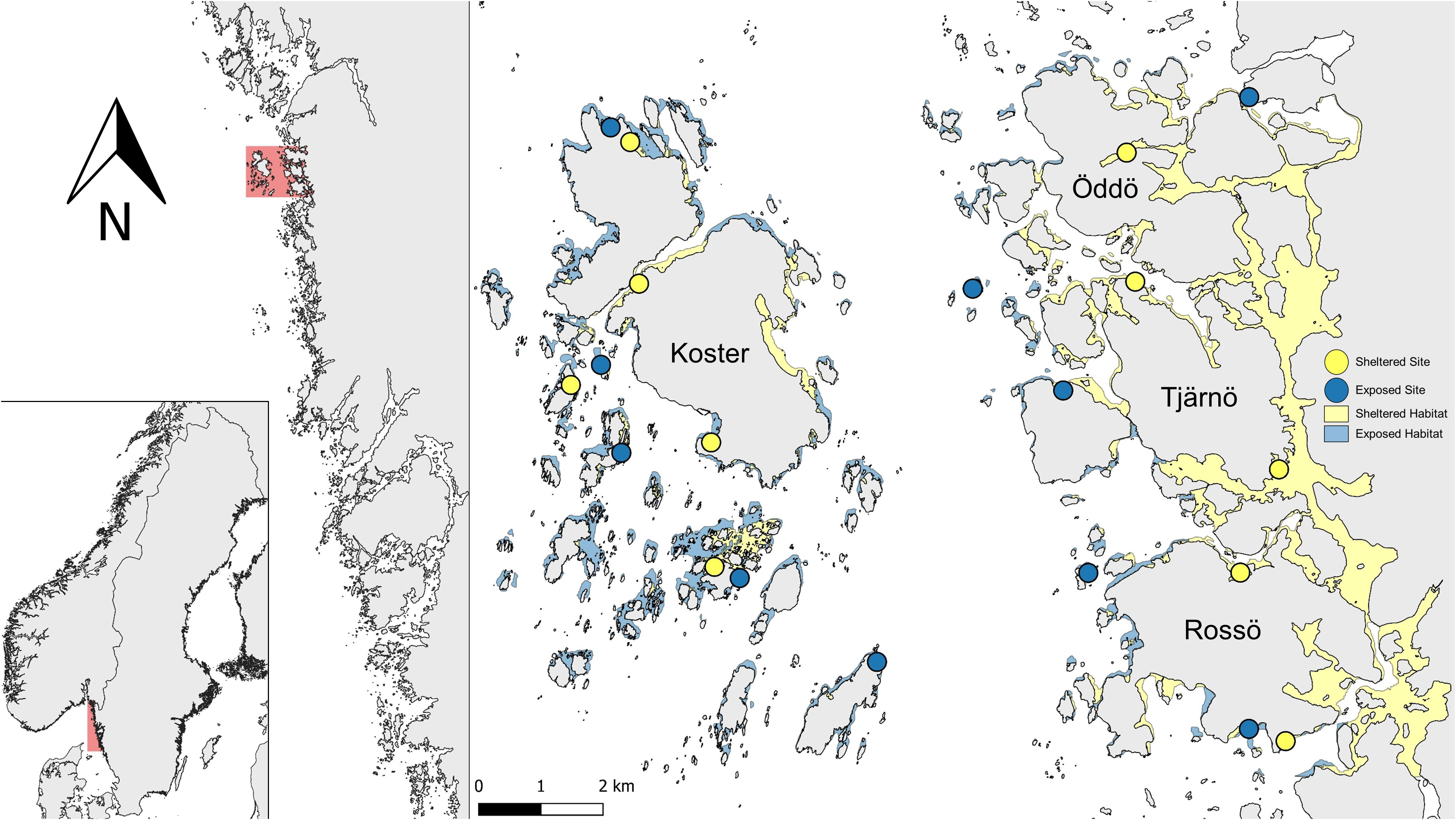
Figure 1 Map of study area and sampling sites on the Swedish west coast. Shallow habitat (<2 m depth) is shown in blue for exposed, and yellow for sheltered. Sampled sites are shown as circles in blue for exposed and yellow for sheltered. Note that small differences in exposure can be obscured by the symbols for sample locations.
The tidal range in this area is small (± 0.3 m), but due to differences in atmospheric pressure and winds the water level may vary by up to 1.0 m. In general, surface salinity varies over the year between 20-30 PSU, and temperature varies among seasons between 0-21°C, but strong spatial gradients in both temperature and salinity are expected to occur within the area. Shallow waters habitats (<2 m deep) in this area are usually near or within small bays and beaches, with a wide variety of substrate conditions ranging from bare rock to silty bottoms. The prevailing wind direction comes from the south-west, which determines the level of wave exposure experienced by any particular stretch of coastline together with its orientation and fetch.
To estimate representatively, abundance and biomass of bivalves in the area, and to evaluate the importance of spatial variability and of selected environmental factors, a total of 20 sites were sampled in the archipelago from the 13th of July to 20th of August 2021. The sites were stratified with respect to area (“Tjärnö” vs “Koster”), wave-exposure (“Sheltered” vs “Exposed”) and depth (“Shallow” vs “Deep”). Potential sampling sites were selected by checking for areas that were shallower than 2 meters with a length of at least 100 meters, using digital nautical charts and satellite images. Wave-exposure was determined from available digital maps of modelled, classified exposure (Albertsson et al., 2006). In total 69 “Sheltered” (ultra-sheltered to very sheltered) and 57 “Exposed” (sheltered – moderately exposed) sites in the “Tjärnö” area and 15 sheltered and 95 exposed sites in the “Koster” area were identified (see Figure 1). Five sites for each level of area and exposure were randomly selected for sampling. Each site was also stratified by depth with “Shallow” samples taken at depths of 0-0.5 m and “Deep” samples between 0.5-2 m. The start- and endpoints of each 100-meter stretch where a site would be sampled were predetermined on the map to avoid selection bias in the field. Working from one point of the 100-meter stretch to the other, one infaunal and one epifaunal sample were taken at about equal intervals (≈10 m) along the shore (n=10 each for epi- and infauna). The exact depth of each sample was assigned using random numbers in order to get representative samples within the defined depth strata. Local tidal level was checked regularly during field work and sampling depth was adjusted accordingly.
At each site, ten epibenthic samples were taken per depth stratum using a 1x1 m metal quadrat, which was laid on the substrate surface, with the middle of the square at the randomly selected sampling depths (n=10). All epibenthic bivalves within the quadrat were collected. “Shallow” samples were collected while wading and “Deep” samples were collected by snorkelling. In each quadrat the percental cover of substrate categories mud, sand, gravel, shell hash and rock were recorded. In a few cases of very dense epibenthic bivalve cover, subsamples of the quadrat were taken instead using smaller quadrats positioned randomly.
Infaunal bivalves were sampled using sediment cores. “Shallow” cores were taken using a PVC tube with a diameter of 30.15 cm (0.07 m2). The cores were pushed ≈20 cm into the sediment or as far as it would go, and the content was dug out and sieved in the field using a sieve with a 4 mm mesh size. “Deep” cores were taken from a small boat using a steel pole corer with a diameter of 9.8 cm (0.008 m2). In order to obtain comparable sampling areas in both depth strata, 9 pole cores (0.068 m2) were taken within a radius of ±1 m at each of the 10 sampling positions. Note that infaunal samples could only be taken at sites where sedimentary habitats were found and therefore these data are partially unbalanced among sites. Bivalve samples were in labelled containers and transported to the Tjärnö Marine Laboratory where they were kept frozen at -20°C until further analysis.
Bivalves were counted and identified to species level when possible. After being allowed to defrost, total wet weight was determined, and soft tissues were removed. The tissue was dried at 40°C for a minimum of 48 hours or until constant in weight. The dry weight was noted and the tissue was then burned at 560°C for 6 hours and weighed again after cooling down in a desiccator. Ash free dry weight (AFDW) was calculated by subtracting the weight of the ash from the dry weight. Occasionally, individuals were too small or broken to remove the flesh reliably. In such situations the tissue was burnt with the shell with the assumption that the weight of the shell would remain constant during the burning procedure and would be subtracted together with the weight of the ash. AFDW and abundance values were standardized to grams and individuals per m2 by dividing them by the surface area of the sample method.
The bivalve communities were described using frequency, biomass and abundance of individual species. In addition, the species composition and its reliance on environmental factors (substrate types and wave-exposure) was assessed at the scale of sites using constrained ordination by distance-based redundancy analysis (dbRDA; Legendre & Anderson, 1999). Tests were performed using distance based multiple regression (DistLM; Mcardle and Anderson, 2001) in PRIMER v6 software with PERMANOVA+ (Anderson et al., 2008). Dissimilarities in species composition among sites were estimated using Bray-Curtis dissimilarities calculated on 4th root transformed abundance data. Three sites (two “Koster-Exposed” and one “Tjärnö-Exposed”) were excluded from this analysis as no bivalves were found at these sites. Quantitative measures of exposure were estimated a posteriori from the mean of the values extracted from the same wave-exposure layer (Albertsson et al., 2006) used to classify the sites at the coordinates of each sample. Exposure, together with the other variables (mean rock, mud, sand, gravel, and hash cover from the quadrat samples) were transformed to and checked for collinearity using the variance inflation factor (VIF; Critical threshold =3). The number of permutations for DistLM was set to 9 999 and a marginal test was used to test significance of environmental factors.
The combined effects of the site classifications Area (Koster, Tjärnö), Exposure (Exposed, Shallow) and Depth (Shallow, Deep) on mean biomass and abundance of infaunal and epifaunal bivalves were tested using analysis of variances (ANOVA, SS type II) with four factors:
where the response variable yijklm is abundance or biomass, Ai is the effect of the ith area, Ej is the jth exposure class, Dk is the kth depth stratum, Site(AE)l(ij) is the lth site within area i and exposure j and ϵijklm is the deviation not explained by any factor or interaction. After inspection of residuals, it was decided to transform biomass and abundance with a log10(y+1) transformation. In the case of the epifauna the total number of samples was 400 (a=2 areas, b=2 exposure levels, c=2 depth strata, d=5 sites, n=10 replicates), but because no infauna samples were taken at locations where the substrate was rocky or in other ways impossible to sample with a core, the data for the infaunal bivalves had less samples (a total of 225) and hence became unbalanced. The same analyses were applied also to the percent cover of the three most important substrate types (Rock, Sand and Mud) that were estimated from the quadra samples. This was done to quantify and test for differences in habitat characteristics among areas, exposures and depths at different sites and the substrate availability for the two groups of bivalves. All statistical analysis was done in R 4.1.3 (R Core Team, 2022) unless otherwise stated.
In order to assess the overall importance of epi- and infaunal bivalves in terms of their biomass and abundance in different environmental contexts (e.g. areas and levels of exposure), estimates of mean bivalve biomass and abundance, , proportions of habitat availability, Pijk , and areal extent of each combination of exposure and area, Arij (in the 0-2 m depth range) were combined. The latter was obtained from a standardized GIS-layer provided by the Swedish authorities (Albertsson et al., 2006). In order to compensate for the fact that shallow and deep samples represented depth ranges of 0-0.5 and 0.5-2 m respectively, estimated abundances were weighted by ¼ and ¾ for the two depths (wi). For infauna the available sedimentary habitat, Pijk , was estimated from quadrat samples (), while for epifauna Pijk =1 as this faunal component is found on both soft and hard substrates (all data are provided in the Supplementary Table S1). The importance of epi- and infaunal bivalves in different environmental contexts were calculated as:
In general, the observations from the quadrats showed that the a priori stratification of exposure- and depth-classes was ecologically meaningful despite being made from GIS-maps (Figure 2). For example, the cover of hard substrata in exposed areas in Tjärnö and Koster ranged from ≈40-80%, with higher values in the shallow stratum as expected. Similarly, mud was exclusively observed at sites classified as sheltered with a predominance at depths between 0.5-2 m (i.e. ≈60 and 30% in Tjärnö and Koster respectively). Sandy sediments were more evenly distributed at levels of 20-40%. These patterns were also largely supported by statistical analyses (Table 1). Thus, significant differences in the cover of rocky, sandy, and muddy substrates between the two exposure levels and depth strata were found (Table 1). Rock was significantly higher in exposed sites and at shallow depth. The patterns of mud opposed that of rock, having more cover in shallow sites and at deeper depth. In general, there were no significant differences of sediment cover between the two areas Koster and Tjärnö, nor interactive effects with exposure and depth, indicating that the quantitative criteria used to define levels of exposure and depth, were in fact comparable in terms of physical impacts in both Tjärnö and Koster. Nevertheless, the significant variability observed among sites for all variables indicates that there were also other uncontrolled variables that influence the substrate characteristics of shallow sites in the study area (Table 1).
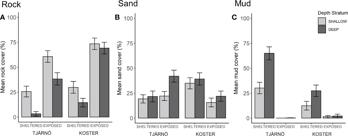
Figure 2 Average cover of rock [(A), including boulders and stones], sand (B) and mud (C) measured using visual inspections in 1x1 m sampling quadrats (mean ± SE).
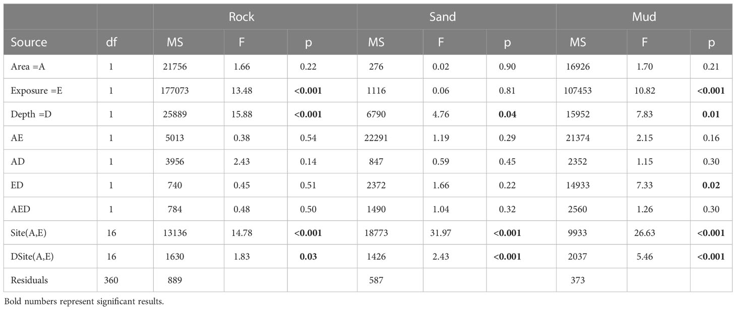
Table 1 Analysis of variance results of the cover of rock (including boulders and stones), sand and mud measured by visual inspection.
In total 17 species of bivalves (11 infaunal and 6 epifaunal) were observed during this study (Table 2). In terms of the number of sites where the species occurred, Mytilus edulis was the most prevalent epifaunal species with a 75% occurrence rate. The most common infaunal species was Polititapes aureus with an occurrence rate of 40% of the sites. While all infaunal and epifaunal species were observed in the Tjärnö area, only 11 species were found in Koster. Overall, the contribution by epifaunal species to the total biomass was considerately larger than that of infauna in both Tjärnö (88%) and Koster (75%) (Table 2). The total biomass of both epifaunal and infaunal bivalves was more than three times higher in Tjärnö compared to Koster (2093 versus 678 grams) and the total abundance, however, was only 1.8 times higher in Tjärnö compared to Koster (3639 versus 2044 individuals).
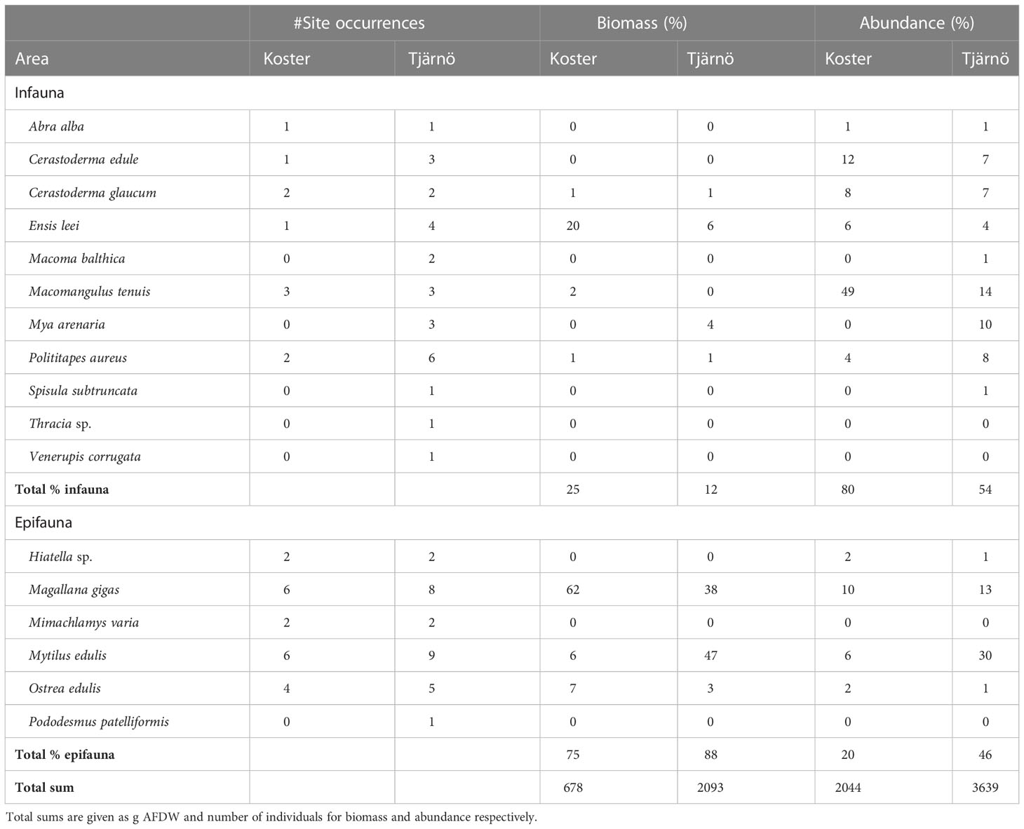
Table 2 Summary of infaunal and epifaunal bivalve species observations: #site occurrences (of a maximum 10), relative biomass and abundance in Tjärnö and Koster.
Visual inspections of the dbRDA-plots did not show any clear separation among areas or exposure classes (Figure 3). If anything, it appeared that the exposed sites in Koster were located in the high end of the second axis (which appears to be associate with large values of exposure and cover of rock; Figure 3B). A total of 36% of the variability was explained by the two first axes and the importance of the first axis was approximately twice that of the second axis (41 vs 24% of the explained variability). Interestingly, all infaunal species tended to be negatively correlated with the first and second axes (excluding species with a correlation coefficient<0.3 and those observed in less than four sites; Figure 3A). This correspond with sites dominated by large cover of sand, gravel and shell hash, but with small cover of rock and independently of mud (Figure 3B). This pattern was further corroborated by the DistLM showing significant correlation between community structure on one hand and exposure, rock and sand on the other (p<0.05; Table S2). Occurrence of epifaunal species were largely correlated by the second axis (Figure 3A). In particular, the native species, Ostrea edulis and Mytilus edulis, were associated with the presence of gravel, while the recently introduced Magallana gigas, appeared to be more of a generalist.
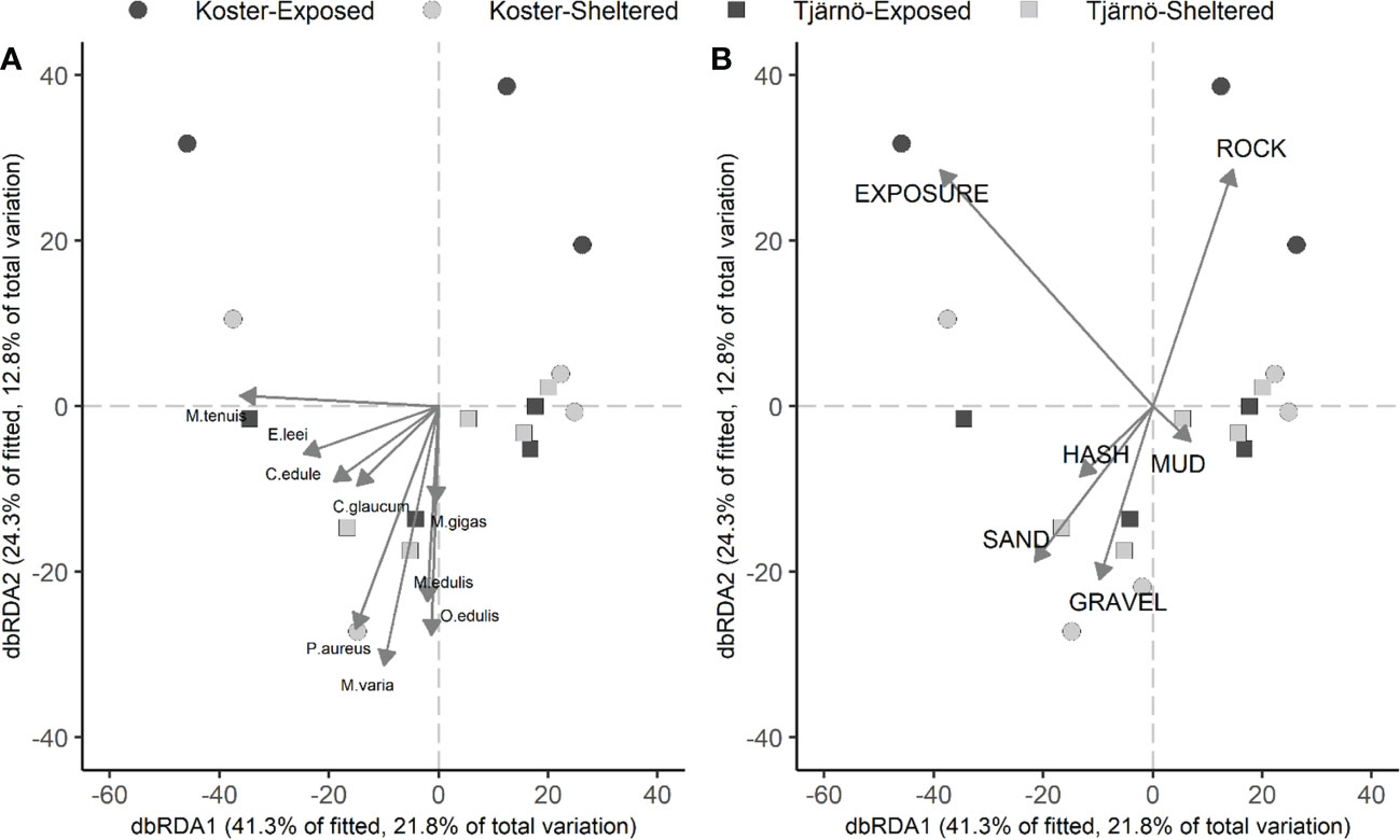
Figure 3 Ordination plots of distance-based redundancy analysis (dbRDA) correlation vectors for (A) species (excluding those occurring at<4 sites and with correlations<0.3, epifaunal indicated represented by bold letters) and (B) environmental variables. Distances are based on Bray-Curtis of 4th root transformed means.
Although the patterns of biomass in relation to depth and exposure appear similar in epi- and infauna, it is clear that the main part of the biomass is associated with the epifaunal species (Figures 4A, C). On average, the epifaunal biomass was ≈7 times larger per square meter (of suitable habitat) than that of the infauna in both levels of exposure in Tjärnö and Koster. In contrast to analyses of substrate characteristics, detailed analyses using ANOVA revealed that patterns of biomass of epi- and infauna were more complex and unpredictable in relation to area, depth and exposure (Table 3). For both types of fauna there was a substantial and significant variability among sites within area and level of exposure. Despite the fact that both types of fauna generally demonstrated larger means in the deeper stratum, this pattern was only fully consistent and significant for infauna.

Figure 4 Average biomass (AFDW g•m-2, A, C) and abundance (#•m-2, B, D) of epifauna (top) and infauna (lower)(mean ± SE). Note the different scales on the response axes between epi- and infauna.
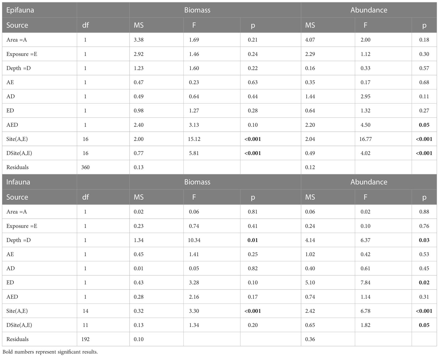
Table 3 Analysis of variance results of biomass (AFDW g·m-2) and abundance (#·m-2) of epi- and infaunal bivalves.
Also, for the spatial patterns of total abundance, there was partial consistency between epi- and infauna (Figures 4B, D). However, the relative importance of the two types of fauna in terms of abundance was reversed compared to that of the biomass. Thus, the average abundance of infauna, in areas where sedimentary habitats were available, was on average ≈3 times that of epifauna. Similarly to biomass, there was substantial variability among sites but there were also complex interactions among the main effects for both epi- and infauna (Table 3). The numerically more important infauna showed a different response to depth in exposed and sheltered areas; infauna was virtually absent at shallow depths in exposed sites. Epifauna on the other hand, was absent all the way down to 2 m in exposed sites in Koster, while in Tjärnö epifauna was most abundant in exposed areas (Figures 4B, D).
While the previous analyses describes the average amount of biomass and abundance of epi- and infauna in different geographic areas and levels of exposure where suitable habitats were present, a more realistic comparison of their importance require that (a) the relative occurrence of sedimentary and rocky habitats (Pijk ) and (b) the areal extent of exposure and geographic strata (ArPij ) are accounted for (Figure 1). These analyses show that the exposed areas in Koster deviate from all other areas with on average small total bivalve biomass and abundance (<1 g and ≈1 # m2 respectively; Figures 5A, B). In all other areas (sheltered areas in Koster and exposed and sheltered areas in Tjärnö), total biomass was on average 8-18 g AFDW/m2 for both depth strata combined. The majority (80-90%) of this biomass consisted of epifauna. This pattern was partly reversed in comparisons of abundance, where sheltered sites in both Tjärnö and Koster were dominated by infauna (≈75%). In exposed areas in Tjärnö, presumably low availability of sedimentary habitats mean that abundances are dominated by epifauna. Moreover, both total biomass and abundance were highest in exposed parts in Tjärnö and sheltered parts in Koster, both of which represents intermediate positions in the longitudinal inshore-offshore gradient in the study area.
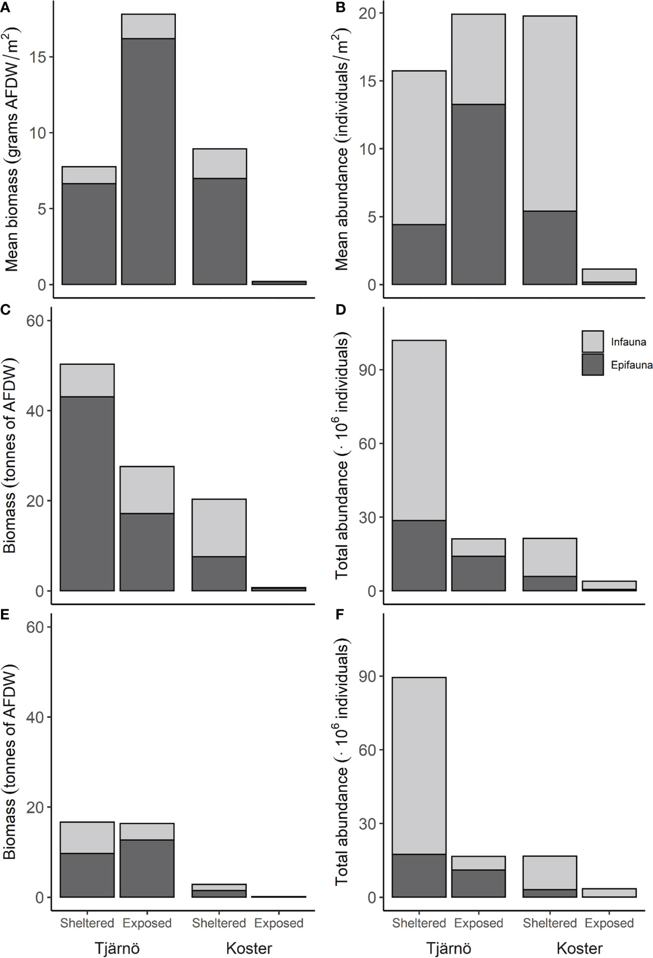
Figure 5 Total biomass (AFDW) and total abundance of epi- and infauna in sheltered and exposed parts of Tjärnö and Koster areas. The first row show biomass (A) and abundance (B) per m2 accounting for habitat availability, and the second row show the totals accounting also for areal extent (C, D). The third row show total biomass (E) and abundance (F) for each area excluding the two invasive species, Magallana gigas and Ensis leei. See text and Table S1 for details about calculations and data.
Finally, in order to assess the potential importance of epi- and infauna, to overall population and ecosystem processes in different parts of this coastal gradient, information on the areal extent of 0-2 m habitats in sheltered and exposed areas in Tjärnö and Koster as quantified (Figures 5C, D). Note that the estimates of areal extent correspond to the somewhat arbitrary boundaries in Figure 1, from which the sampling sites were randomly selected (data on areal extent are given in Table S1). The calculations show that the contribution of the areas to the total bivalve biomass and abundance decrease in a similar way: Tjärnö (sheltered)> Tjärnö (exposed)> Koster (sheltered)> Koster (exposed) (Figures 5C, D). This pattern was of course partly explained by the fact that Tjärnö (sheltered) contributed with ≈54% of the area, which offsets the slightly lower estimates of total biomass and abundances compared to when data were expressed per square m (Figure 5). Note also that the second largest area (Koster (exposed) at ≈29%) had a negligible contribution to bivalve total biomass and abundance while the intermediately located areas, which where the smallest (≈9% each), contributed substantially.
The general aim of this study was to quantify the distribution and abundance of bivalves in a wide range of benthic environments on the Swedish Skagerrak coast, with the goal to assess the potential of epi- and infaunal species as contributors to ecological processes and ultimately ecosystem services. In order to achieve this, the abundance and biomass of both epibenthic and infaunal bivalve communities were sampled and the data was combined with data on habitat availability and with GIS derived data on areal extent of the sampled habitats. This resulted in several new insights about the ecological importance of bivalves, in a range of coastal environments, and in the region as a whole, but also illustrated the benefits of structured sampling which enabled comparisons among faunal components and up-scaling of results to provide a system-wide comparison and assessment. This study addresses a major gap in knowledge on the relative importance of epi- and infaunal bivalves in terms of biomass and abundance. The ecological and methodological insights are also useful in a local, as well as a more general context.
Depth was found to be of significant importance for the distribution of infaunal biomass. However, contrary to what was predicted, there were no significant differences for depth for epifauna and exposure and area for both in- and epifauna, even though there were remarkable differences between then in terms of absolute numbers. This is a result of the significant unexplained variation between sites, which seems to indicate that there are more complex patterns and processes that shape the bivalve communities in this area that were not captured in this study. One striking result of this study is that epifaunal bivalves were the dominant group in terms of average biomass per unit area in both Tjärnö and Koster. At the time of the study, there was ≈100 tonnes of bivalve biomass in the whole area (100 AFDW/0.8≈124 tonnes of shell free dry weight or 100/0.07≈1 400 tonnes of wet weight; conversion factors from Rumohr et al., 1987). 70% of the biomass was epifauna and 30% was infauna. The amount of biomass was highly variable among sites, but in general larger biomass was found at depths between 0.5-2 m both for infauna and epifauna. Accounting for the uneven distribution of infaunal habitat (measured as 100% rock), the highest bivalve biomass (10-15 g·m-2) occurs in the intermediate parts of the coastal gradient, i.e. in the exposed parts of Tjärnö and in the sheltered part of Koster areas, followed by the inner, sheltered parts of Tjärnö (≈8 g·m-2). Finally, scaling up these results using GIS-estimates of the extent of sheltered and exposed areas at 0-2 m depth, show that sheltered habitats in the inner parts of the archipelago contribute with ≈50% of the biomass in this region. Despite the fact that >90% of the deeper and ≈80% of the shallow parts of this area is covered by sediments, infaunal bivalves only contribute to 10-15% of the biomass.
The biomass data presented here are representative for this region and the specific depth ranges and exposures levels that were included in this study. This type of sampling differs from previous studies done on the Swedish west coast, which had different objectives and have typically focused on smaller geographical areas and usually include either epi- or infaunal bivalves. Perhaps the most comparable data available is presented in Evans and Tallmark, 1977; Möller and Rosenberg, 1983 and Loo and Rosenberg, 1989. Firstly, Evans and Tallmark, 1977 found epifaunal biomass of 7.1 and 3.1 g AFDW·m-2 at one site in two consecutive years, compared to 5-15 g AFDW·m-2 in this study. The infaunal portion of the biomass in this study was also lower (3.1 and 0.3 g AFDW·m-2, 0-3 g AFDW·m-2 in this study). Secondly, in Möller and Rosenberg, 1983 biomass of two infaunal species varied over a six-year period at two sites depending on the survival of the recruitment of the previous year, but was most often between 1 and 10 g AFDW·m-2 around the same time of year of this study. It was also found that there was generally more biomass deeper than 0.5 meter than above it. Lastly, Loo and Rosenberg, 1989 reports about 22 and 5.5 g AFDW·m-2 (converted from WW with factors from Rumohr et al., 1987) of infaunal bivalve biomass at two sites. It must be clear that because of the differences in methods and objectives a comparison between those studies is not entirely correct. Nonetheless, it can be concluded that the finding on biomass per area reported here fall within the ranges that have been reported previously, which supports the validity of the results of this survey. In contrast this study allowed for up-scaling and direct comparison between epi- and infaunal bivalves.
Although the relationships between biomass and filtration-rate or -capacity is non-linear and modulated by environmental factors and behavioral responses of bivalves, and despite the fact that measurement of filtration is complex in laboratory- and field-experiments, it is clear that the biomass of an individual or a bivalve community is a fundamental indicator of its filtration capacity (e.g. Kryger & Riisgård, 1988; and reviewed in Riisgård, 2001). Furthermore, because several critical ecosystem functions and processes are linked to filtration (e.g. water clearance, nutrient uptake and cycling and production), the observed patterns of biomass arguably have important implications also for many ecosystem services. First, the results indicate that overall, epifauna (mainly Magallana gigas, Mytilus edulis and Ostrea edulis) contributes to a larger extent to water clearance and removal of nutrients compared to infaunal species. This is true considering the total biomass per square meter in sampled sites but also when considering the areal extent of sheltered and exposed habitats in Tjärnö and Koster. Nevertheless, in certain sites, particularly at intermediate areas in the in- and offshore gradient, the contribution made by infaunal bivalves such as, Ensis leei, Mya arenaria and Macomangulus tenuis, appeared to match that of the epifauna. Studies targeting both functional groups with suitable sampling regimes in soft and rocky habitats, particularly those accounting for areal extent, are scarce (but see for example Seitz et al., 2006), but it has been found before that the contribution of biomass per unit area is greater for epifauna in Swedish coastal areas (Evans & Tallmark, 1977).
From the biomass we are able to conclude that the filtration capacity of both epi- and infaunal bivalves is markedly smaller in the exposed parts of Koster. While the scarcity of sedimentary habitat explains the low levels of infauna, the low biomass of epifauna is more surprising. Particularly because of the large densities of epifaunal biomass at similarly exposed areas in Tjärnö, which illustrates that the species can withstand such levels of hydrodynamic forces (note also that the very to extremely exposed areas in Koster were excluded from the study). Thus, in order to explain the lack of filter-feeding biomass in exposed areas in Koster, more complex models including factors correlated with the physical aspects of wave-exposure and the inshore – offshore gradient needs to be invoked. In general, such factors may include supply of food, supply of larvae, fluctuations in salinity and temperature or sedimentation (e.g. Lindegarth & Gamfeldt, 2005; Westerbom & Jattu, 2006; Lindegarth, 2007) but here, low epifaunal bivalve biomass (and abundance) could possibly be explained by waves modulating the effects of ecological interactions (e.g. competition, predation or “algal swiping”) acting on larvae, juveniles or adult bivalves (e.g. Underwood, 1999). Nevertheless, whatever the mechanism, it is clear that the end result of these patterns is a large difference among sheltered and exposed areas in their contribution to bivalve biomass and by extension to regulating services associated with filtration. These results emphasize the need to incorporate knowledge about the distribution and abundance of fauna, availability of habitats and areal extent when assessing relative contributions to ecological processes and ultimately to different types of ecosystem services. It is particularly interesting to note that, while the inner parts of this coastal gradient appear to contribute most both in terms of biomass and abundance, the relative importance of the two functional components are practically reversed.
In general, the overall spatial patterns of density and total abundance resembles that of the biomass, however, in contrast to what was observed for the biomass the main part of abundance was made up of infauna rather than epifauna. While the epifaunal abundance, mainly consisted of two species (Mytilus edulis and Magallana gigas), infaunal abundance was more diverse and variable among habitats. In Koster the abundance was dominated by the tellinid, Macomangulus tenuis, the cockles Cerastoderma edule and C. glaucum. In Tjärnö, the same species and two additional ones (Mya arenaria and Polititapes aureus) were mainly observed, and in general the species abundance was more evenly distributed. Possibly, this can be attributed to the more exposed nature of the Koster islands, causing a thinner margin of suitable sediment and environmental conditions for infaunal species. The multivariate analyses showed that most infaunal species were positively correlated with sandy and gravelly sediments rather than those dominated by mud, which is common to sites in the sheltered parts of Tjärnö. It is possible that here the areal extend of this type of sediment is greater than in Koster, and probably less likely to be subjected to events of extreme wave energy, allowing for a more diverse assemblage of bivalves to occur.
While it can be argued that the contribution of bivalve to certain ecosystem services depends on the filter-feeding capacity and hence mainly on the biomass, others services are more closely linked to abundance and species composition. For example, the habitat forming role of epibenthic mussels and oysters and the importance for associated biodiversity is mainly dependent on their abundance and not primarily on the amount of filter-feeding tissue. Although abundances of epifauna was substantially smaller than that of infauna, particularly when accounting for the large areal extent of sheltered habitats in Tjärnö, they were abundant enough to form unique and particularly valuable biotopes (e.g. both mussel- and oyster-beds are included on the “OSPAR list of threatened and/or declining species and habitats”, OSPAR, 2008), and they provide substrate, shelter and foraging area for many associated invertebrates and fish species (e.g. Humphries et al., 2011; P. Norling et al., 2015; P. Norling & Kautsky, 2007). Note that this role of epifauna, supporting and maintaining biodiversity is potentially important both in rocky and sedimentary habitats. In contrast, infauna performs ecological functions exclusively burrowing in sedimentary habitats. Although less conspicuous than the epibenthic species, infaunal species can also act as ecosystem engineers by reworking the sediment, modifying small-scale topography and oxygen conditions (Rosenberg, 2001; Norkko and Shumway, 2011). Furthermore, many infaunal species in shallow habitats are important food-sources for e.g. wading birds. Large abundances of juvenile or adult infaunal bivalves attract and support a rich variety of birds specialized on feeding on bivalves, supporting terrestrial biodiversity and providing a pathway for energy and nutrient transfer to non-marine systems (van Roomen et al., 2012).
Despite exceeding that of epifauna, the overall infaunal abundances were lower compared to data available from previous studies in the sampled area (e.g. Lindegarth et al., 1995). It is unlikely that this observation was a sampling artefact as the number of cores taken at each site in this study was evaluated to be sufficient to ensure that the probability of false negatives for occurrences of bivalves was acceptably low. For common infaunal species such the two cockle species Cerastoderma edule and C. glaucum, from these previous studies it was expected to find average densities of about 1-10 individuals·m-2. Taking 20 samples from each site (i.e. 1.4 m2) and assuming a Poisson distribution, this would amount to an average probability of false negatives of 50, 25 and<1% for densities of 0.5, 1 and 10 individuals·m-2. Average densities of the two Cerastoderma species were, however, found to be on the order of 0.1 individuals·m-2, i.e. one to two orders of magnitude smaller than expected. Both infauna abundance and biomass in this study appeared much lower compared to studies done in studies done in other areas (e.g. Beukema et al., 2001; Seitz et al., 2006). In the case of Beukema et al., 2001, our data corresponds with the absolute minimums in their area during a sampling period spanning over 25 years. Although these systems differ from the area in this study in for instance tidal ranges and the availability of shallow soft sediment habitat, the comparisons are remarkable and suggest fundamental differences in filter-feeding biomass that are related to these conditions. More data and analyses are necessary to assess whether this is a persistent long-term change in this area or part of natural fluctuation.
Population of infaunal bivalves are known to show strong temporal fluctuations, usually caused by mass die-offs (Burdon et al., 2014), which can be caused by several reasons, and subsequent increases after favorable years of new settlement (Beukema et al., 2001). From the current data, it is unclear whether there is in fact a substantial decline or if the observations made are normal fluctuations in abundances. The cause of such a decline, if unordinary, can be speculated. Earlier monitoring has revealed that this area has had increased occurrences of dense mats of filamentous algae in the genus Cladophora (Pihl et al., 1995). These algae spread quickly in protected bays in the summer months and persist for many weeks. These locations correspond well with habitat that is usually associated with infaunal bivalve species such as Cerastoderma spp. and Mya arenaria. Algae mats like these can theoretically smother infauna bivalves, restricting their access to food and oxygen (Perkins and Abbott, 1972). Another possible cause is an increase in the abundance of mesopredators that feed on juvenile bivalve spat (Möller and Rosenberg, 1983; Flach, 2003).
One interesting and potentially important result from this study is that both epi- and infaunal bivalve communities were dominated by invasive species, Magallana gigas and Ensis leei, particularly in terms of biomass. The total biomass was estimated to ≈100 tonnes AFDW (69 and 31 for epi- and infauna respectively). If M. gigas and E. leei are excluded, only ≈35% of the epifaunal and ≈40% of the infaunal biomass remains. Thus, assuming that these establishments have occurred without any competitive exclusion or otherwise caused decrease of native species, these two species have added 60-65% of filter-feeding biomass to this coastal area. Although these assumptions cannot be automatically accepted (see below), these are substantial contributions to benthic-pelagic coupling processes, particularly in sheltered parts of the Tjärnö area. Consequently, it can be argued that these changes may have had substantial effects on ecosystem functioning in these habitats, as for instance the Pacific oyster that has introduced a new source of habitat formation service to the region.
The Pacific oyster Magallana gigas (Thunberg 1793) is well known invasive species (Ruesink et al., 2005) and since its introduction to western Europe in the 1960’s, it has come to dominate coastal communities that were favored habitat for the native blue mussel Mytilus edulis (Fey et al., 2010; Holm et al., 2016; Reise et al., 2017). This study has shown that also in shallow habitats in the northern west coast of Sweden, it is now the dominating bivalve species. Current status of Pacific oysters on the Swedish west coast has developed comparatively recent, after a wide scale recruitment event observed in 2006 (Wrange et al., 2010). This event coincided with warm summer temperatures (Wrange et al., 2010) and based on DNA evidence (Faust et al., 2017), it is presumed to be a natural dispersal event. Prior reports of declining blue mussel populations in this area are thus unlikely to be attributed to the recent rise of the Pacific oyster (Baden et al., 2021). Pacific oysters now also appears to overlap considerably with the native and endangered flat oyster, Ostrea edulis (Linnaeus 1758) in the study area (Bergström et al., 2021). During this study these three species where often observed growing communally within the same cluster. Other studies report Pacific oysters living in what appears to be stable association with blue mussels (Reise et al., 2017) and flat oysters (Zwerschke et al., 2016; Christianen et al., 2018). This implies that there are interactions between Pacific oysters and the native oyster and mussel species, although the developments are too recent and there is done insufficient research to foresee how the invaders presence will affect the native species in Sweden in the long term.
Even though the arrival of the Atlantic jackknife clam Ensis leei (Huber 2015) was much earlier than that of the Pacific oyster, i.e. in the early 1980’s, much less is known about its route of invasion, in which habitats it now occurs and what the overall impact has been on the local benthic ecosystems. Similar to the Pacific oyster, the American jackknife clam has a wide salinity tolerance range (7-32 PSU, Maurer et al., 1974), and thus has invaded many varieties of coastal habitats in Europe to the extent where it is also dominating communities along the south-eastern coast of the North Sea and the Wadden Sea (Gollasch et al., 2015). In accordance, these results show this invader contributed to the largest part of the infaunal bivalve biomass in the study area. Like other studies describing its preferred habitat, it was encountered predominantly in clean, fine-grained sand in the sublittoral zone (Armonies and Reise, 1998; Beukema and Dekker, 1995). The species can form very dense assemblages, where it increases the accumulation of silt and organic content in the sediment (Dannheim and Rumohr, 2012), thus causing indirect changes to the benthic community (Armonies and Reise, 1998). Although there are no local extinctions of other species attributed to the arrival of the American jackknife clam, it coincides with a decline in other infaunal species along the Belgian and Dutch North Sea coast (Dekker and Beukema, 2012; Houziax et al., 2009). Additionally, it has been observed that in areas where it has become common, bivalve eating birds have made a switch to this new food source (Cadée, 2000, Caldow et al., 2007, Tulp et al., 2010). Future research should aim to map the distribution of this species further and investigate how it affects the native bivalve communities and coastal ecosystems in this area.
Scaling up spatial patterns of biodiversity and understanding ecological interactions at the landscape level is a vital component for increasing the fundamental understanding of ecological functions and systems (e.g. Duarte et al., 2005; Kutti et al., 2013; Lohrer et al., 2015; Gonzalez et al., 2020), and for monitoring, conserving and restoring marine habitats (e.g. Schoch & Dethier, 1996; Bayraktarov et al., 2020). One manifestation of this is the recent increase in studies using empirical models often linked to remote sensing methods to predict and map the geographic distribution of species or habitats (e.g. He et al., 2015; Breiner et al., 2018). A wide variety of techniques (e.g. species distribution models (SDMs)) are available to predict both categorical (e.g. presence vs absence of species or habitats) and quantitative responses (e.g. abundance, biomass or rates of processes). In order be sufficiently powerful and precise these techniques require large amounts of data and access to suitable GIS-layers of relevant predictor variables.
In this study area, reliable GIS data of sufficient resolution was not available, particularly for substrate characteristics. Furthermore, sampling abundance and biomass of epi- and infaunal bivalves at a sufficient number of sites (i.e. ≈100 sites) for these more sophisticated models to be useful was not feasible. One limitation of this study is that the data collection is limited to a single year, when it is well documented that bivalve population tend to fluctuate annually. This means that the patterns we observed in this study could potentially vary on a yearly basis. Sampling all sites within the area in a short time frame does on the other hand ensure that these temporal changes do not cause uncertainties when combining data from several years, which potentially could obscure some of the patterns that were found in this study. By excluding temporal variation, it proved to be an efficient way to estimate and explore effects of exposure and depth on bivalves and habitats associated to these factors, and allowed us to evaluate random variability within and among sites.
Furthermore, by adopting a “top-down” approach (e.g. Hewitt et al., 2004), it was also possible to scale-up these representative samples and assess the importance of filter-feeding bivalves over the whole archipelago area, which is characterized by strong environmental gradients of wave-exposure, depth and a complex mosaic of soft and rocky habitats. Thus, despite not being able to predict and map biomass and abundance with a detailed resolution (e.g. at a resolution of 5-10 m), instead it was opted to make robust inferences about the importance of epi- and infaunal species at the scale of this coastal landscape, without having to rely on finding powerful and precise models. Key to this was the deliberate strategy to use a random sampling design, within objectively defined strata with known areal extent. Note, however, that data collected in this way can readily be used for more detailed prediction and mapping, in the event that sufficient data and GIS-information becomes available (e.g. Guillera-Arroita et al., 2015; Guisan et al., 2017; Breiner et al., 2018).
In conclusion, a sampling strategy based on (1) representative sampling, (2) a combination of appropriate sampling methods in soft and rocky habitats and (3) use of GIS for stratification and up-scaling, provided a robust framework for estimating the importance of benthic species in coastal landscapes. It was found that epifaunal species, overall, contributed significantly more to the total bivalve biomass in shallow coastal waters in the northern part of the Swedish west coast, and thus, most probably are chiefly responsible for the many ecosystem services associated with suspension feeding bivalves such as water quality and nutrient cycling. Although infaunal species amounted to less biomass in total, their abundances at certain sites still indicated these species are influencing local sediment processes and functions, especially in areas of intermediate exposure. Additionally, with these methods it was possible to give valuable information on the status of two invasive species who appear to dominate their respective functional groups in terms of biomass, and are now likely major contributors to the ecosystem functions and services related to suspension feeding and habitat formation.
The raw data supporting the conclusions of this article will be made available by the authors, without undue reservation.
All authors were involved in the conceptualization and planning of the field work as well as contextualizing the results. YG was responsible for preforming the field and lab work and data preparation. The statistical analysis was done by YG and ML. PB has done the GIS work involving the selection of sample sites, calculations for the areal analysis and preparing layers to produce the figures. The manuscript was written mainly by YG and ML, with contribution from PB and ÅS. All authors contributed to the article and approved the submitted version.
The authors declare that the research was conducted in the absence of any commercial or financial relationships that could be construed as a potential conflict of interest.
All claims expressed in this article are solely those of the authors and do not necessarily represent those of their affiliated organizations, or those of the publisher, the editors and the reviewers. Any product that may be evaluated in this article, or claim that may be made by its manufacturer, is not guaranteed or endorsed by the publisher.
The Supplementary Material for this article can be found online at: https://www.frontiersin.org/articles/10.3389/fmars.2023.1105999/full#supplementary-material
Albertsson J., Bergström U., Isaeus M., Kilnäs M., Lindblad C., Mattisson A., et al. (2006). Sammanställning och Analys av Kustnära Undervattenmiljö (Report 5591). Naturvårdsverket.
Aller R. (1988). “Benthic fauna and biogeochemical processes in marine sediments: the role of burrow structures,” in Nitrogen cycling in coastal marine environments, 301–338.
Anderson M. J., Gorley R. N., Clarke K. R. (2008). PERMANOVA+ primer V7: User manual. Prim. Ltd. Plymouth UK.
Armonies W., Reise K. (1998). On the population development of the introduced razor clam Ensis americanus near the island of Sylt (North Sea). Helgolander Meeresuntersuchungen 52, 291–300. doi: 10.1007/BF02908903.
Baden S., Hernroth B., Lindahl O. (2021). Declining populations of mytilus spp. in north atlantic coastal waters - A Swedish perspective. J. Shellfish Res. 40, 269–296. doi: 10.2983/035.040.0207.
Barbier E. B., Hacker S. D., Kennedy C., Koch E. W., Stier A. C., Silliman B. R. (2011). The value of estuarine and coastal ecosystem services. Ecol. Monogr. 81, 169–193. doi: 10.1890/10-1510.1
Bayraktarov E., Brisbane S., Hagger V., Smith C. S., Wilson K. A., Lovelock C. E., et al. (2020). Priorities and motivations of marine coastal restoration research. Front. Mar. Sci. 7. doi: 10.3389/fmars.2020.00484
Beadman H. A., Kaiser M. J., Galanidi M., Shucksmith R., Willows R. I. (2004). Changes in species richness with stocking density of marine bivalves. J. Appl. Ecol. 41, 464–475. doi: 10.1111/j.0021-8901.2004.00906.x
Beck M. W., Brumbaugh R. D., Airoldi L., Carranza A., Coen L. D., Crawford C., et al. (2011). Oyster reefs at risk and recommendations for conservation, restoration, and management. Bioscience 61, 107–116. doi: 10.1525/bio.2011.61.2.5
Bergström P., Thorngren L., Strand Å., Lindegarth M. (2021). Identifying high-density areas of oysters using species distribution modeling: Lessons for conservation of the native ostrea edulis and management of the invasive magallana (Crassostrea) gigas in Sweden. Ecol. Evol. 11, 5522–5532. doi: 10.1002/ece3.7451
Bersoza Hernández A., Brumbaugh R. D., Frederick P., Grizzle R., Luckenbach M. W., Peterson C. H., et al. (2018). Restoring the eastern oyster: how much progress has been made in 53 years? Front. Ecol. Environ. 16, 463–471. doi: 10.1002/fee.1935
Beukema J. J., Dekker R., Essink K., Michaelis H. (2001). Synchronized reproductive success of the main bivalve species in the wadden Sea: Causes and consequences. Mar. Ecol. Prog. Ser. 211, 143–155. doi: 10.3354/meps211143
Beukema J. J., Dekker R. (1995). Dynamics and Growth of a Recent Invader in to European Coastal Waters: The American Razor Clam, Ensis Directus. J. Mar. Biol. Assoc. United Kingdom 75, 351–362. doi: 10.1017/S0025315400018221.
Bouma T. J., Olenin S., Reise K., Ysebaert T. (2009). Ecosystem engineering and biodiversity in coastal sediments: Posing hypotheses. Helgol. Mar. Res. 63, 95–106. doi: 10.1007/s10152-009-0146-y
Bouma J. A., Van Beukering P. J. H. (2015). Ecosystem services: From concept to practice. (Cambridge: Cambridge University Press). doi: 10.1017/CBO9781107477612
Breiner F. T., Nobis M. P., Bergamini A., Guisan A. (2018). Optimizing ensembles of small models for predicting the distribution of species with few occurrences. Methods Ecol. Evol. 9, 802–808. doi: 10.1111/2041-210X.12957
Burdon D., Callaway R., Elliott M., Smith T., Wither A. (2014). Mass mortalities in bivalve populations: A review of the edible cockle cerastoderma edule (L.). Estuar. Coast. Shelf Sci. 150, 271–280. doi: 10.1016/j.ecss.2014.04.011
Cadée G. C. (2000). Herring gulls feeding on a recent invader in the Wadden Sea, Ensis directus. Geol. Soc. Spec. Publ. 177, 459–464. doi: 10.1144/GSL.SP.2000.177.01.31.
Caldow R., Stillman R. A., West A. D. (2007). Modelling study to determine the capacity of The Wash shellfish stocks to support eider Somateria mollissima. Nat. Engl. Res. Reports 83, 265.
Christianen M. J. A., Lengkeek W., Bergsma J. H., Coolen J. W. P., Didderen K., Dorenbosch M., et al. (2018). Return of the native facilitated by the invasive? population composition, substrate preferences and epibenthic species richness of a recently discovered shellfish reef with native European flat oysters (Ostrea edulis) in the north Sea. Mar. Biol. Res. 14, 590–597. doi: 10.1080/17451000.2018.1498520
Christianen M. J. A., van der Heide T., Holthuijsen S. J., van der Reijden K. J., Borst A. C. W., Olff H. (2017). Biodiversity and food web indicators of community recovery in intertidal shellfish reefs. Biol. Conserv. 213, 317–324. doi: 10.1016/j.biocon.2016.09.028
Ciutat A., Widdows J., Pope N. D. (2007). Effect of cerastoderma edule density on near-bed hydrodynamics and stability of cohesive muddy sediments. J. Exp. Mar. Bio. Ecol. 346, 114–126. doi: 10.1016/j.jembe.2007.03.005
Cloern J. E., Abreu P. C., Carstensen J., Chauvaud L., Elmgren R., Grall J., et al. (2016). Human activities and climate variability drive fast-paced change across the world’s estuarine-coastal ecosystems. Glob. Change Biol. 22, 513–529. doi: 10.1111/gcb.13059
Coen L. D., Brumbaugh R. D., Bushek D., Grizzle R., Luckenbach M. W., Posey M. H., et al. (2007). Ecosystem services related to oyster restoration. Mar. Ecol. Prog. Ser. 341, 303–307. doi: 10.3354/meps341303
Costanza R., D’Arge R., de Groot R., Farber S., Grasso M., Hannon B., et al. (1997). The value of the world’s ecosystem services and natural capital. Nature 387, 253–260. doi: 10.1038/387253a0
Dannheim J., Rumohr H. (2012). The fate of an immigrant: Ensis directus in the eastern German Bight. Helgol. Mar. Res. 66, 307–317. doi: 10.1007/s10152-011-0271-2.
Dekker R., Beukema J. J. (2012). Long-term dynamics and productivity of a successful invader: The first three decades of the bivalve Ensis directus in the western Wadden Sea. J. Sea Res. 71, 31–40. doi: 10.1016/j.seares.2012.04.004.
Díaz S., Pascual U., Stenseke M., Martín-López B., Watson R. T., Molnár Z., et al. (2018). Assessing nature’s contributions to people. Sci. (80-. ). 359, 270–272. doi: 10.1126/science.aap8826
Duarte C. M., Dennison W. C., Orth R. J. W., Carruthers T. J. B. (2008). The charisma of coastal ecosystems: Addressing the imbalance. Estuaries Coasts 31, 233–238. doi: 10.1007/s12237-008-9038-7
Duarte C. M., Middelburg J. J., Caraco N. (2005). Major role of marine vegetation on the oceanic carbon cycle. Biogeosciences 2, 1–8. doi: 10.5194/bg-2-1-2005
Ehrnsten E., Norkko A., Müller-Karulis B., Gustafsson E., Gustafsson B. G. (2020). The meagre future of benthic fauna in a coastal sea–benthic responses to recovery from eutrophication in a changing climate. Glob. Change Biol. 26, 2235–2250. doi: 10.1111/gcb.15014
Evans S., Tallmark B. (1977). Growth and biomass of bivalve molluscs on a shallow, sandy bottom in gullmar fjord (Sweden). Zoon 5, 33–38.
Falkowski P. G., Barber R. T., Smetacek V. (1998). Biogeochemical controls and feedbacks on ocean primary production. Sci. (80-. ). 281, 200–206. doi: 10.1126/science.281.5374.200
Faust E., André C., Meurling S., Kochmann J., Christiansen H., Jensen L. F., et al. (2017). Origin and route of establishment of the invasive Pacific oyster Crassostrea gigas in Scandinavia. Mar. Ecol. Prog. Ser. 575, 95–105. doi: 10.3354/meps12219.
Fey F., Dankers N., Steenbergen J., Goudswaard K. (2010). Development and distribution of the non-indigenous Pacific oyster (Crassostrea gigas) in the Dutch Wadden Sea. Aquac. Int. 18, 45–59. doi: 10.1007/s10499-009-9268-0.
Flach E. C. (2003). The separate and combined effects of epibenthic predation and presence of macro-infauna on the recruitment success of bivalves in shallow soft-bottom areas on the Swedish west coast. J. Sea Res. 49, 59–67. doi: 10.1016/S1385-1101(02)00199-5
Forêt M., Barbier P., Tremblay R., Meziane T., Neumeier U., Duvieilbourg E., et al. (2018). Trophic cues promote secondary migrations of bivalve recruits in a highly dynamic temperate intertidal system. Ecosphere 9. doi: 10.1002/ecs2.2510
Gollasch S., Kerckhof F., Craeymeersch J., Goulletquer P., Jensen K., Jelmert A., et al. (2015). Alien species alert: Ensis directus. current status of invasions by the marine bivalve ensis directus. ICES Coop. Res. Rep. 323, 36. doi: 10.17895/ices.pub.5491
Gómez-Baggethun E., de Groot R., Lomas P. L., Montes C. (2010). The history of ecosystem services in economic theory and practice: From early notions to markets and payment schemes. Ecol. Econ. 69, 1209–1218. doi: 10.1016/j.ecolecon.2009.11.007
Gonzalez A., Germain R. M., Srivastava D. S., Filotas E., Dee L. E., Gravel D., et al. (2020). Scaling-up biodiversity-ecosystem functioning research. Ecol. Lett. 23, 757–776. doi: 10.1111/ele.13456
Gosling E. (2004). Bivalve molluscs: Biology, ecology, and culture. (Oxford, UK: Blackwell Publishing Ltd) doi: 10.1002/9780470995532
Grabowski J. H., Brumbaugh R. D., Conrad R. F., Keeler A. G., Opaluch J. J., Peterson C. H., et al. (2012). Economic valuation of ecosystem services provided by oyster reefs. Bioscience 62, 900–909. doi: 10.1525/bio.2012.62.10.10
Guillera-Arroita G., Lahoz-Monfort J. J., Elith J., Gordon A., Kujala H., Lentini P. E., et al. (2015). Is my species distribution model fit for purpose? matching data and models to applications. Glob. Ecol. Biogeogr. 24, 276–292. doi: 10.1111/geb.12268
Guisan A., Thuiller W., Zimmermann N. E. (2017). Habitat suitability and distribution models: with applications in R (Cambridge, UK: Cambridge University Press). doi: 10.1017/9781139028271.011
Guy-Haim T., Lyons D. A., Kotta J., Ojaveer H., Queirós A. M., Chatzinikolaou E., et al. (2018). Diverse effects of invasive ecosystem engineers on marine biodiversity and ecosystem functions: A global review and meta-analysis. Glob. Change Biol. 24, 906–924. doi: 10.1111/gcb.14007
Hansen K., King G. M., Kristensen E. (1996). Impact of the soft-shell clam mya arenaria on sulfate reduction in an intertidal sediment. Aquat. Microb. Ecol. 10, 181–194. doi: 10.3354/ame010181
Harley C. D. G., Hughes A. R., Hultgren K. M., Miner B. G., Sorte C. J. B., Thornber C. S., et al. (2006). The impacts of climate change in coastal marine systems. Ecol. Lett. 9, 228–241. doi: 10.1111/j.1461-0248.2005.00871.x
He K. S., Bradley B. A., Cord A. F., Rocchini D., Tuanmu M. N., Schmidtlein S., et al. (2015). Will remote sensing shape the next generation of species distribution models? Remote Sens. Ecol. Conserv. 1, 4–18. doi: 10.1002/rse2.7
Hewitt J. E., Thrush S. F., Legendre P., Funnell G. A., Ellis J., Morrison M. (2004). Mapping of marine soft-sediment communities: Integrated sampling for ecological interpretation. Ecol. Appl. 14, 1203–1216. doi: 10.1890/03-5177
Holm M. W., Davids J. K., Dolmer P., Holmes E., Nielsen T. T., Vismann B., et al. (2016). Coexistence of Pacific oyster Crassostrea gigas (Thunberg, 1793) and blue mussels Mytilus edulis (Linnaeus, 1758) on a sheltered intertidal bivalve bed? Aquat. Invasions 11, 155–165. doi: 10.3391/ai.2016.11.2.05.
Houziax J. S., Craeymeersch J., Merckx B., Kerckhof F., Van Lancker V., Courtens W., et al. (2009). ‘EnSIS’ - Ecosystem Sensitivity to Invasive Species (Final Report). Belgian Science Policy.
Humphries A. T., Ayvazian S. G., Carey J. C., Hancock B. T., Grabbert S., Cobb D., et al. (2016). Directly measured denitrification reveals oyster aquaculture and restored oyster reefs remove nitrogen at comparable high rates. Front. Mar. Sci. 3. doi: 10.3389/fmars.2016.00074
Humphries A. T., La Peyre M. K., Kimball M. E., Rozas L. P. (2011). Testing the effect of habitat structure and complexity on nekton assemblages using experimental oyster reefs. J. Exp. Mar. Bio. Ecol. 409, 172–179. doi: 10.1016/j.jembe.2011.08.017
Jackson J. B. C., Kirby M. X., Berger W. H., Bjorndal K. A., Botsford L. W., Bourque B. J., et al. (2001). Historical overfishing and the recent collapse of coastal ecosystems. Sci. (80-. ). 293, 629–637. doi: 10.1126/science.1059199
Kellogg M. L., Smyth A. R., Luckenbach M. W., Carmichael R. H., Brown B. L., Cornwell J. C., et al. (2014). Use of oysters to mitigate eutrophication in coastal waters. Estuar. Coast. Shelf Sci. 151, 156–168. doi: 10.1016/j.ecss.2014.09.025
Kryger J., Riisgård H. U. (1988). Filtration rate capacities in 6 species of European freshwater bivalves. Oecologia 77, 34–38. doi: 10.1007/BF00380921
Kutti T., Bannister R. J., Fosså J. H. (2013). Community structure and ecological function of deep-water sponge grounds in the traenadypet MPA-northern Norwegian continental shelf. Cont. Shelf Res. 69, 21–30. doi: 10.1016/j.csr.2013.09.011
Legendre P., Anderson M. J. (1999). Distance-based redundancy analysis: Testing multispecies responses in multifactorial ecological experiments. Ecol. Monogr. 69, 1–24. doi: 10.1890/0012-9615(1999)069[0001:DBRATM]2.0.CO;2
Lindegarth M. (2007). “Wave exposure,” in Encyclopedia of tidepools (Berkeley: USA: University of California Press), 630–633.
Lindegarth M., Andre C., Jonsson P. R. (1995). Analysis of the spatial variability in abundance and age structure of two infaunal bivalves, cerastoderma edule and c.lamarcki, using hierarchical sampling programs. Mar. Ecol. Prog. Ser. 116, 85–98. doi: 10.3354/meps116085
Lindegarth M., Dunér Holthuis T. T. L., Bergström P., Lindegarth S. (2014). Ostron (Ostrea edulis) i kosterhavets nationalpark: kvantitativa skattningar och modellering av förekomst och totalt antal (Report 2014:43). Länsstyrelsen i Västra Götalands län, Naturvårdsenheten. doi: 10.13140/RG.2.1.1933.1280
Lindegarth M., Gamfeldt L. (2005). Comparing categorical and continuous ecological analyses: Effects of “wave exposure” on rocky shores. Ecology 86, 1346–1357. doi: 10.1890/04-1168
Lohrer A. M., Thrush S. F., Hewitt J. E., Kraan C. (2015). The up-scaling of ecosystem functions in a heterogeneous world. Sci. Rep. 5, 1–10. doi: 10.1038/srep10349
Loo L. O., Rosenberg R. (1989). Bivalve suspension-feeding dynamics and benthic-pelagic coupling in an eutrophicated marine bay. J. Exp. Mar. Bio. Ecol. 130, 253–276. doi: 10.1016/0022-0981(89)90167-6
Lotze H. K., Lenihan H. S., Bourque B. J., Bradbury R. H., Cooke R. G., Kay M. C., et al. (2006). Depletion degradation, and recovery potential of estuaries and coastal seas. Sci. (80-. ). 312, 1806–1809. doi: 10.1126/science.1128035
MacKenzie C. L. J., Burrell V. G. J., Rosenfield A., Hobart W. L. (1997). The history, present condition, and future of the molluscan fisheries of north and centeral America and Europe. NOAA Tech. Rep. NMFS 127, 223–234.
Martínez M. L., Intralawan A., Vázquez G., Pérez-Maqueo O., Sutton P., Landgrave R. (2007). The coasts of our world: Ecological, economic and social importance. Ecol. Econ. 63, 254–272. doi: 10.1016/j.ecolecon.2006.10.022
Maurer D., Watling L., Aprill G. (1974). The distribution and ecology of common marine and estuarine pelecypods in the Delaware Bay Area. The Nautilus 88(2):38–46.
Mcardle B. H., Anderson M. J. (2001). Fitting multivariate models to community Data : A comment on distance-based redundancy analysis. Ecology 82, 290–297. doi: 10.1890/0012-9658(2001)082[0290:FMMTCD]2.0.CO;2
McLeod I. M., zu Ermgassen P. S. E., Gillies C. L., Hancock B., Humphries A., Westby S. R., et al. (2019). “Can Bivalve Habitat Restoration Improve Degraded Estuaries?” in Coasts and Estuaries: The Future (Amsterdam, The Netherlands: Elsevier Inc.), 427–442. doi: 10.1016/B978-0-12-814003-1.00025-3
Meadows P. S., Meadows A., Murray J. M. H. (2012). Biological modifiers of marine benthic seascapes: Their role as ecosystem engineers. Geomorphology 157–158, 31–48. doi: 10.1016/j.geomorph.2011.07.007
Möller P., Rosenberg R. (1983). Recruitment, abundance and production of mya arenaria and cardium edule in marine shallow waters, Western Sweden. Ophelia 22, 33–55. doi: 10.1080/00785326.1983.10427223
Newell R. I. E. (2004). Ecosystem influences of natural and cultivated populations of suspension-feeding bivalve molluscs: A review. J. Shellfish Res. 23, 51–61. doi: 10.2983/035.029.0302
Newell R. I. E., Cornwell J. C., Owens M. S. (2002). Influence of simulated bivalve biodeposition and microphytobenthos on sediment nitrogen dynamics: A laboratory study. Limnol. Oceanogr. 47, 1367–1379. doi: 10.4319/lo.2002.47.5.1367
Norkko A., Hewitt J. E., Thrush S. F., Funnell G. A. (2001). Benthic-pelagic coupling and suspension-feeding bivalves: Linking site-specific sediment flux and biodeposition to benthic community structure. Limnol. Oceanogr. 46, 2067–2072. doi: 10.4319/lo.2001.46.8.2067
Norkko A., Hewitt J. E., Thrush S. F., Funnell G. A., Norkko A., Hewitt J. E., et al. (2006). Conditional outcomes of facilitation by a habitat-modifying subtidal bivalve. Ecology 87, 226–234. doi: 10.1890/05-0176
Norkko J., Shumway S. E. (2011). “Bivalves as bioturbators and bioirrigators,” in Shellfish aquaculture and the environment (Hoboken, New Jersey: Wiley Science Publishers), 297–317. doi: 10.1002/9780470960967.ch10
Norling P., Kautsky N. (2007). Structural and functional effects of mytilus edulis on diversity of associated species and ecosystem functioning. Mar. Ecol. Prog. Ser. 351, 163–175. doi: 10.3354/meps07033
Norling P., Lindegarth M., Lindegarth S., Strand A. (2015). Effects of live and post-mortem shell structures of invasive pacific oysters and native blue mussels on macrofauna and fish. Mar. Ecol. Prog. Ser. 518, 123–138. doi: 10.3354/meps11044
Norling K., Rosenberg R., Hulth S., Grémare A., Bonsdorff E. (2007). Importance of functional biodiversity and species-specific traits of benthic fauna for ecosystem functions in marine sediment. Mar. Ecol. Prog. Ser. 332, 11–23. doi: 10.3354/meps332011
OSPAR (2008) Case reports for the OSPAR list of threatened and/or declining species and habitats. Available at: https://qsr2010.ospar.org/media/assessments/p00358_case_reports_species_and_habitats_2008.pdf.
Perkins E. J., Abbott O. J. (1972). Nutrient enrichment and sand flat fauna. Mar. pollut. Bull. 3, 70–72. doi: 10.1016/0025-326X(72)90162-2
Peterson B. J., Heck K. L. (2001). An experimental test of the mechanism by which suspension feeding bivalves elevate seagrass productivity. Mar. Ecol. Prog. Ser. 218, 115–125. doi: 10.3354/meps218115
Pihl L., Isaksson I., Wennhage H., Moksnes P. O. (1995). Recent increase of filamentous algae in shallow Swedish bays: Effects on the community structure of epibenthic fauna and fish. Netherlands J. Aquat. Ecol. 29, 349–358. doi: 10.1007/BF02084234
Prins T. C., Smaal A. C., Dame R. F. (1997). A review of the feedbacks between bivalve grazing and ecosystem processes. Aquat. Ecol. 31, 349–359. doi: 10.1023/A:1009924624259
Ramesh R., Chen Z., Cummins V., Day J., D’Elia C., Dennison B., et al. (2015). Land-ocean interactions in the coastal zone: Past, present & future. Anthropocene 12, 85–98. doi: 10.1016/j.ancene.2016.01.005
R Core Team (2022) R: A language and environment for statistical computing. Available at: https://www.r-project.org/.
Reise K., Buschbaum C., Büttger H., Rick J., and Wegner K. M. (2017). Invasion trajectory of Pacific oysters in the northern Wadden Sea. Mar. Biol. 164, 1–14. doi: 10.1007/s00227-017-3104-2
Riisgård H. U. (2001). On measurement of filtration rates in bivalves - the stony road to reliable data: Review and interpretation. Mar. Ecol. Prog. Ser. 211, 275–291. doi: 10.3354/meps211275
Riisgård H. U., Lassen J., Kortegaard M., Møller L. F., Friedrichs M., Jensen M. H., et al. (2007). Interplay between filter-feeding zoobenthos and hydrodynamics in the shallow odense fjord (Denmark) - earlier and recent studies, perspectives and modelling. Estuar. Coast. Shelf Sci. 75, 281–295. doi: 10.1016/j.ecss.2007.04.032
Rosenberg R. (2001). Marine benthic faunal sucessional stages and related sedimentary activity. Sci. Mar. 65, 107–119. doi: 10.3989/scimar.2001.65s2107
Ruesink J. L., Lenihan H. S., Trimble A. C., Heiman K. W., Micheli F., Byers J. E., et al. (2005). Introduction of non-native oysters: Ecosystem effects and restoration implications. Annu. Rev. Ecol. Evol. Syst. 36, 643–689. doi: 10.1146/annurev.ecolsys.36.102003.152638.
Rumohr H., Brey T., Ankar S. (1987). A compilation of biometric conversion factors for benthic invertebrates of the Baltic Sea (Kiel, Germany: Institut für Meereskunde).
Sandwell D. R., Pilditch C. A., Lohrer A. M. (2009). Density dependent effects of an infaunal suspension-feeding bivalve (Austrovenus stutchburyi) on sandflat nutrient fluxes and microphytobenthic productivity. J. Exp. Mar. Bio. Ecol. 373, 16–25. doi: 10.1016/j.jembe.2009.02.015
Schoch G. C., Dethier M. N. (1996). Scaling up: The statistical linkage between organismal abundance and geomorphology on rocky intertidal shorelines. J. Exp. Mar. Bio. Ecol. 201, 37–72. doi: 10.1016/0022-0981(95)00167-0
Seitz R. D., Lipcius R. N., Olmstead N. H., Seebo M. S., Lambert D. M. (2006). Shoreline development and benthic diversity. Mar. Ecol. Prog. Ser. 326, 11–27. doi: 10.3354/meps326011
Smaal A. C., Ferreira J. G., Grant J., Petersen J. K., Strand Ø. (2018). Goods and services of marine bivalves. (Cham, Switzerland: Springer International Publishing). doi: 10.1007/978-3-319-96776-9
Sueiro M. C., Bortolus A., Schwindt E. (2011). Habitat complexity and community composition: Relationships between different ecosystem engineers and the associated macroinvertebrate assemblages. Helgol. Mar. Res. 65, 467–477. doi: 10.1007/s10152-010-0236-x
Tulp I., Craeymeersch J., Leopold M., van Damme C., Fey F., Verdaat H. (2010). The role of the invasive bivalve Ensis directus as food source for fish and birds in the Dutch coastal zone. Estuar. Coast. Shelf Sci. 90, 116–128. doi: 10.1016/j.ecss.2010.07.008.
Underwood A. J. (1999). Physical disturbances and their direct effect on an indirect effect: Responses of an intertidal assemblage to a severe storm. J. Exp. Mar. Bio. Ecol. 232, 125–140. doi: 10.1016/S0022-0981(98)00105-1
van der Schatte Olivier A., Jones L., Vay L., Christie M., Wilson J., Malham S. K. (2020). A global review of the ecosystem services provided by bivalve aquaculture. Rev. Aquac. 12, 3–25. doi: 10.1111/raq.12301
van der Zee E. M., Angelini C., Govers L. L., Christianen M. J. A., Altieri A. H., van der Reijden K. J., et al. (2016). How habitat-modifying organisms structure the food web of two coastal ecosystems. Proc. R. Soc B Biol. Sci. 283. doi: 10.1098/rspb.2015.2326
van Roomen M., Laursen K., van Turnhout C., van Winden E., Blew J., Eskildsen K., et al. (2012). Signals from the wadden sea: Population declines dominate among waterbirds depending on intertidal mudflats. Ocean Coast. Manage. 68, 79–88. doi: 10.1016/j.ocecoaman.2012.04.004
Velasco-Charpentier C., Pizarro-Mora F., Navarro N. P., Valdivia N. (2021). Disentangling the links between habitat complexity and biodiversity in a kelp-dominated subantarctic community. Ecol. Evol. 11, 1214–1224. doi: 10.1002/ece3.7100
Westerbom M., Jattu S. (2006). Effects of wave exposure on the sublittoral distribution of blue mussels mytilus edulis in a heterogeneous archipelago. Mar. Ecol. Prog. Ser. 306, 191–200. doi: 10.3354/meps306191
Whitlatch R. B., Hines A. H., Thrush S. F., Hewitt J. E., Cummings V. (1997). Benthic faunal responses to variations in patch density and patch size of a suspension-feeding bivalve. J. Exp. Mar. Bio. Ecol. 216, 171–189. doi: 10.1016/S0022-0981(97)00095-6
Wiberg P. L., Taube S. R., Ferguson A. E., Kremer M. R., Reidenbach M. A. (2019). Wave attenuation by oyster reefs in shallow coastal bays. Estuaries Coasts 42, 331–347. doi: 10.1007/s12237-018-0463-y
Wrange A. L., Valero J., Harkestad L. S., Strand Ø., Lindegarth S., Christensen H. T., et al. (2010). Massive settlements of the pacific oyster, crassostrea gigas, in Scandinavia. Biol. Invasions 12, 1453–1458. doi: 10.1007/s10530-009-9565-6
zu Ermgassen P. S. E., Spalding M. D., Grizzle R. E., Brumbaugh R. D. (2013). Quantifying the loss of a marine ecosystem service: Filtration by the Eastern oyster in US estuaries. Estuaries Coasts 36, 36–43. doi: 10.1007/s12237-012-9559-y
Keywords: survey, biodiversity, infauna, epifauna, invasive species, mussels, oysters, functional groups
Citation: Greeve Y, Bergström P, Strand Å and Lindegarth M (2023) Estimating and scaling-up biomass and abundance of epi- and infaunal bivalves in a Swedish archipelago region: Implications for ecological functions and ecosystem services. Front. Mar. Sci. 10:1105999. doi: 10.3389/fmars.2023.1105999
Received: 23 November 2022; Accepted: 09 January 2023;
Published: 24 January 2023.
Edited by:
Renato Crespo Pereira, Fluminense Federal University, BrazilReviewed by:
Kevin Alexander Hovel, San Diego State University, United StatesCopyright © 2023 Greeve, Bergström, Strand and Lindegarth. This is an open-access article distributed under the terms of the Creative Commons Attribution License (CC BY). The use, distribution or reproduction in other forums is permitted, provided the original author(s) and the copyright owner(s) are credited and that the original publication in this journal is cited, in accordance with accepted academic practice. No use, distribution or reproduction is permitted which does not comply with these terms.
*Correspondence: Youk Greeve, eW91ay5ncmVldmVAZ3Uuc2U=
Disclaimer: All claims expressed in this article are solely those of the authors and do not necessarily represent those of their affiliated organizations, or those of the publisher, the editors and the reviewers. Any product that may be evaluated in this article or claim that may be made by its manufacturer is not guaranteed or endorsed by the publisher.
Research integrity at Frontiers
Learn more about the work of our research integrity team to safeguard the quality of each article we publish.