Effects of ocean states coupling on the simulated Super Typhoon Megi (2010) in the South China Sea

Responses of the South China Sea (SCS) to a typhoon are complex due to the susceptible upper layer and active multiscale motions and thus need to be urgently resolved and validated in numerical simulations. A coupled atmosphere–ocean–wave model and various in-situ observations were applied to understand the strong interactions between Super Typhoon Megi (2010) and the SCS, especially the wave effects on typhoon simulation. Five sensitive experiments using different combinations of models were firstly conducted and compared to validate the effectiveness of the ocean coupling. Compared with WRF-only and ROMS-only outputs, the coupled experiments evidently improved the accuracy of typhoon intensity, the typhoon-induced cold wake, and significant wave height, along with the thermodynamical responses in the upper 400 m layer, including the near-inertial currents, the variation in ocean heat content, and mixed layer depth. However, the differences between WRF-ROMS and COAWST were slight, though the significant wave height was more than 9 m high in COAWST. Further analysis showed that the modification of heat flux, which could cancel out the effect due to the wave-induced surface roughness, is consistent with that of momentum flux in the wave-coupled experiment. This resulted in similar overall results. To further figure out the wave effects on typhoon and eliminate the contingency brought by the surface physical parameterization scheme, six experiments using three surface physical parameterization schemes were designed with and without wave coupling, separately. The sensible heat flux showed significant differences between three schemes, followed by the latent heat flux and the correspondingly changing momentum loss. Results support the above-mentioned conclusion that the typhoon intensity was determined by the net surface flux. Our findings highlight the necessity in using a high-resolution coupled atmosphere–ocean–wave model and proper surface physical parameterization, especially when coupling waves to make accurate regional numerical environment predictions.

1 Introduction

Tropical cyclones (TCs) are extreme weather disasters that cause severe casualties and property damage to coastal areas worldwide, and are particularly frequent in the Western Pacific Ocean (WP) (D’Asaro et al., 2011). Under the context of the increasing ocean warmth with global warming, TC climates are changing, i.e., increasing in intensity and decreasing in frequency over the past 30 years (Kang and Elsner, 2015). Therefore, it is becoming even more important to improve the accuracy of forecasting TC track and intensity, as well as storm surges and ocean waves to support the mission of protecting lives and property in coastal regions. It is well-recognized that the TC intensity is strongly modulated by air–sea interactions due to the feedback of upper ocean response (Price, 1981) and the pre-existing ocean states, such as mesoscale eddies and pre-TC ocean mixed layer thickness topography (Jaimes and Shay, 2009). To improve forecasting, a better understanding of the effects of ocean states on simulations of TC is required.

The South China Sea (SCS), located on the edge of the Northwest Pacific Ocean (NWP), is an almost enclosed basin with narrow straits connecting both Pacific and Indian Oceans. With its highly complex topography and relatively unique meteorological and changing hydrological environments, the SCS is one of the most sensitive regions to weather and climate change in the Northern Hemisphere and an area with frequent TC activities (Wang et al., 2007). Since typhoon-induced wind stress may lead to significant changes in SCS circulation and near-inertial oscillation (Guan et al., 2014; Ko et al., 2014), frequent typhoons may further enhance the complexity of the ocean environment in the SCS conversely. The ocean responses to a typhoon over the NWP differs significantly from one that passes over the SCS since the mixed layer in the SCS is generally shallower than that in the NWP (Thompson and Tkalich, 2014; Mei et al., 2015) with the interactions between complex motion of various scales being more active, such as the strong internal tides (Guan et al., 2014). Therefore, more significant surface temperature variations can occur than in the deep open NWP (Qu et al., 1997). Unlike NWP, the complex background ocean environment in the SCS may have a complex modulation effect on the response of the upper ocean to typhoons, which increases the difficulty of forecast and has drawn much interest in decades (Chu et al., 2000; Tseng et al., 2010; Chen et al., 2012; Ko et al., 2014).

Typhoon Megi was among the most severe TCs in the SCS with a maximum 10-m wind speed of 72 m s⁻¹. After passing through Luzon into the SCS, it took a large turn and followed an essentially northward track, and induced an intense cold wake (Ko et al., 2014) with a large size and a subcritically slow translation speed. Researchers have conducted various studies on the ocean response to Megi during this process. Through numerical simulation experiments by the ocean model three-dimensional Price-Weller-Pinke (3D PWP) only, and by controlling the TC size, translation speed, or ocean upwelling (Li and Wen, 2017; Pun et al., 2018), they noted that the noticeable sea surface cooling (SSC) in the upper layer of the SCS induced by Megi can be attributed to strong upwelling associated with vertical entrainments in the shallower thermocline. The characteristics of observed and simulated near-inertial oscillation and cold wake were also studied by a simply coupled atmosphere–ocean model (Guan et al., 2014; Ko et al., 2014). Wu et al. (2016) used the coupled WRF and 1D or 3D PWP model to simulate the process of Typhoon Megi in NWP and SCS, respectively, and the results show that the simulation in SCS could be close to the observation only in the 3D model, which indicates the importance of considering advection processes in simulation. These studies illustrate a strong interaction between Typhoon Megi and the ocean.

However, coupling of the ocean to the atmosphere could not be enough to understand the interactions between TCs. In order to understand the physical processes through the air–sea interface during extreme weather like typhoons in the SCS and to improve typhoon forecasting, high-resolution regional coupled atmosphere–ocean–wave models have been employed for extensive studies and found to effectively improve the simulation of wind speed, overall storm evolution and structure of TC, and the thermal and dynamical characteristics of the ocean response (Liu et al., 2012; Chen et al., 2013; Wu et al., 2018; Lim Kam Sian et al., 2020; Sun et al., 2021). Although coupling ocean state has been proven to be useful, the influence of coupling waves on simulated TC intensity is uncertain. Waves’ feedback onto TCs occurs through modulating upper ocean mixing (Zhou et al., 2019) as well as modifying the heat and momentum exchange between air and sea by generating sea sprays and adjusting sea surface roughness (Holthuijsen et al., 2012; Lim Kam Sian et al., 2020). When coupling waves under high wind conditions, stronger mixing may enhance ocean cooling and give negative feedback to TC intensity, while sea sprays produced by surface wave breaking might have a positive effect on TC intensity by increasing the heat flux to the atmosphere and reduction of drag coefficient (Liu et al., 2012; Chen et al., 2013). Therefore, the effect of coupling waves when simulating TCs needs to be further clarified (Liu et al., 2022).

In order to investigate the effects of fully atmosphere–ocean–wave coupling on simulated TC and understand how ocean states coupling improves the accuracy of simulation, we chose Typhoon Megi as the research object and set two groups of experiments, including five sensitive experiments using different combinations of component models, and six experiments using three surface physical parameterization methods in the MYNN scheme with coupled models. The rest of the paper is organized as follows. The data, methods used to optimize the simulation, and experiment settings will be described in Section 2. In Section 3, results and analysis will be provided to validate the effectiveness of coupling ocean states in simulating Megi by comparing experiments and observations. The discussion on the effect of coupling waves in typhoon simulation will be presented in Section 4. Conclusions and discussion will follow in Section 5.

2 Data and methods

2.1 Data

The data used in this paper include TC trajectories and intensities, satellite-derived sea surface temperature (SST) maps, atmospheric and ocean reanalysis, mooring observation, and Argo profiles.

TC information was obtained from the CMA Tropical Cyclone Data Center (China Meteorological Administration, https://tcdata.typhoon.org.cn/en/zjljsjj_sm.html), including the best track, locations of TC center, maximum sustained wind speeds, and minimum central pressure (Lu et al., 2021).

SST maps were retrieved from the Remote Sensing Systems [microwave and infrared merged OI SST product (MW+IR), https://www.remss.com/measurements/sea-surface-temperature/oisst-description/], which provides cloud penetrating daily SST with a resolution of 9 km × 9 km.

The HYCOM reanalysis results (GLBv0.08/expt_53.X) in the SCS were used to analyze the SSC. The data have a spatial resolution of 1/12° and a temporal interval of 3 h, which are available from https://www.hycom.org/data/glbv0pt08/expt-53ptx. The HYCOM reanalysis (GLBu0.08/expt_19.1) used to initialize the ocean conditions in ROMS was downloaded from https://www.hycom.org/data/glbu0pt08/expt-19pt1.

Temperature and salinity profiles were obtained from the Argo datasets passed through quality control, provided by the China Argo Real-time Data Center (http://www.argo.org.cn/). Four Argo floats (A1, A2, A3, and A4) near the track of Typhoon Megi were chosen, with details shown in Figure 1.

FIGURE 1

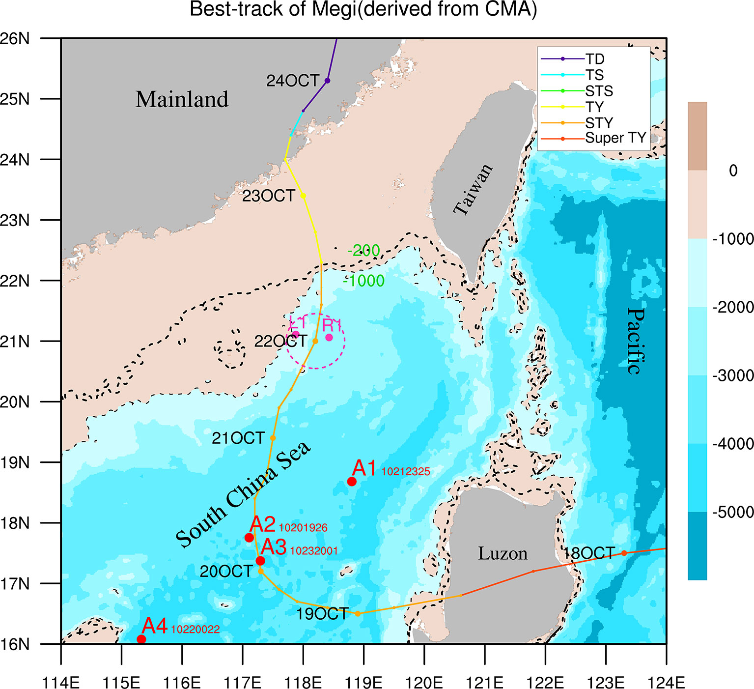
Figure 1 Best track of Typhoon Megi (2010) and topography of the SCS (contour, black dashed line: −200 m and −1,000 m). Different colors of the curve and points stand for different intensities according to the Chinese National Standard for Grade of Tropical Cyclones. Magenta dots represent the positions of moorings (L1: 117°52.66’E, 21°06.57’N; R1: 118°25.61’E, 21°03.59’N), and red dots represent the positions of recorded Argo floats (A1: 118.8030°E, 18.6820°N; A2: 117.1080°E, 17.7550°N; A3: 117.2930°E, 17.3730°N; A4: 115.3280°E, 16.0760°N). The double maximum wind radius of Megi at 00 UTC on 22 October is indicated by the dashed magenta circle.

As part of the South China Sea Internal Wave Experiment (SCSIWEX), two moorings (L1 and R1) were deployed in the northern SCS (Figure 1) from August 2010 to April 2011 (Guan et al., 2014). The center of Typhoon Megi, as a severe typhoon, passed between moorings L1 and R1 at 00 UTC on 22 October, with a relatively slow translation speed of 2.4 m s⁻¹ and a maximum sustained 10-m wind speed of 45 m s⁻¹. Moorings L1 and R1 were approximately 38 km to the left and 26 km to the right of the typhoon track, respectively.

The moorings were equipped with 75 kHz ADCP (Acoustic Doppler Current Profilers) at approximately 400 to 500 m, as well as temperature chains, to measure upper ocean velocity, temperature, and salinity. All of the ADCPs sampled the upper ocean in 8-m bins and formed ensembles every 3 or 5 min. The sampling time interval of the temperature chain was 1 min, with 10-m vertical resolution. Thus, the moorings L1 and R1 contributed to the deeper layer observations, but mooring L1 was equipped only with ADCP and mooring R1 was equipped with both ADCP and temperature chain. Detailed information about each mooring is shown in Figure 1.

2.2 Model and experimental design

2.2.1 Atmospheric model: WRF

The WRF model is a non-hydrostatic, quasi-compressible atmospheric model, with many options available for each physical process, and has been widely used in numerical experiments and forecasts (Skamarock et al., 2008).

In this study, the WRF model was initialized at 00 UTC on 19 October 2010, on the basis of ERA5 reanalysis (Hersbach et al., 2017; Hersbach et al., 2020) with a 0.25° horizontal resolution and 1-h time interval. Terrain data from the University Corporation for Atmospheric Research (UCAR) with a 2-min horizontal resolution were also used to construct the initial and boundary fields. The nested two-way feedback grid was deployed, covering the SCS, from 105°E to 130°E and 8°N to 30°N. The resolution of the outer grid was 9 km and that of the inner grid was 3 km with moving nesting. There were 48 layers in the vertical direction of WRF with the model top of 50 hPa.

Due to the low resolution of ERA5 reanalysis data, the initial vortex of Typhoon Megi was generally weak and poorly positioned. To reflect the real initial vortex intensity and structure, the bogussing scheme, a revised technique (Davis and Low-Nam, 2001), was firstly used. It could detect the vortex by calculating the vorticity near the given location and remove the vorticity anomaly, and relocate an axisymmetric vortex based on the best track data.

To further improve the simulation for typhoon track and intensity, the spectral nudging (SN) technique (Waldron et al., 1996; Von Storch et al., 2000; Guo and Zhong, 2017) was further applied to horizontal winds for all layers of the ERA5 data. A nudging coefficient of 0.0002 s⁻¹ was used for all the nudging variables. A wave number of 2 and 3 was used for the zonal direction and the meridional direction, respectively, and hence, waves with wavelengths equal to or greater than approximately 1,200 km were nudged. This approach considers small-scale information due to the interaction between large-scale atmospheric flows and small-scale geographical features (e.g., topography). Forcing is present at the side boundaries and in the interior and can be retained by adding a nudging term to the frequency domain, effective for large scales while not affecting small scales.

2.2.2 Oceanic model: ROMS

The ROMS model is a free-surface, terrain-following, three-dimensional ocean model that solves the hydrostatic primitive equations for momentum by using a split-explicit time-stepping scheme (Shchepetkin and McWilliams, 2005). A stretched terrain-following coordinate is used in ROMS to discretize the primitive equations over variable topography in the vertical direction. These coordinates allow higher resolutions over the study area.

The ROMS was initialized with the output of HYCOM GLBu0.08/expt_19.1 with the resolution of 1/12° globally. Topographic data ETOPO2 (2-minute Gridded Global Relief Data) were also used to construct the initial and boundary fields. The ROMS domain spans 8–30°N and 105–130°E with a grid resolution of 1/26° × 1/26°. Twenty-four levels were used in the vertical for the stretched terrain-following coordinate with the following vertical stretching parameters: Vtransform = 2, Vstretching = 4, θs = 6.0, θ_b = 0.5, TCLINE = 150, and h = 2000 (where θs is the surface stretching parameter, θ_b is the bottom stretching parameter, TCLINE is thermocline depth in m, and h is the maximum depth in m). The western and eastern lateral boundaries were set to periodic. The tidal forcing along the periodic boundaries was from TPXO tidal data of the Oregon State University (OSU), containing isotropic tidal information with a 0.25° horizontal resolution.

When ROMS runs alone, the atmospheric forcing field is provided by ERA5 reanalysis, while when coupled, the forcing field is provided by the atmospheric model WRF.

2.2.3 Wave model: SWAN

The SWAN model (Booij et al., 1999), a third-generation wave model, is used to simulate wave-induced surface roughness from surface wind and the effects of surface waves.

For the present study, the model grids for SWAN were the same as for ROMS. It is hot-started, where the boundary field uses the WW3 global wave data provided by NCEP (National Centers for Environmental Prediction), containing wave height, wave direction, and wave period, with a 0.5° resolution. When SWAN runs alone, the wind forcing field is from ERA5 reanalysis, but when coupled, the wind field is provided by the atmospheric model WRF.

2.2.4 The fully coupled atmosphere–ocean–wave model

The fully coupled atmosphere–ocean–wave model used in this paper is COAWST developed by Warner et al. (2010) at the Woods Hole Oceanographic Institution, containing the mesoscale atmospheric model WRF, the regional ocean model ROMS, and the wave model SWAN, which proved to be suitable for simulating waves nearshore. All component models are coupled by the MCT toolkit and data are exchanged every 9 min during the coupling process.

During the simulation, the WRF model provides the ocean model ROMS with 10-m winds, atmospheric pressure, relative humidity, and other atmospheric variables such as precipitation and longwave and shortwave radiation, and receives SST from ROMS. At the same time, WRF provides the 10-m wind field to drive the wave model SWAN, which affects the wavefield and in turn receives the wave height and wavelength from SWAN to calculate the sea surface roughness.

Waves also significantly impact the currents through the radiative stresses forcing seawater and mass transport due to Stokes drift and wave-enhanced bottom stresses. At the same time, currents also have a complex impact on waves and affect the wave balance in two ways, either by currents modifying the 10-m wind field of the atmospheric model and thus causing changes in the source term wind stress or by currents modifying the group velocity and then affecting the wave elements. Therefore, the SWAN model provides ROMS with the wave height, wavelength, direction, period, and other information, and receives the current velocities, free surface lift, and depth (bathymetry).

2.2.5 Experimental designs

The simulation was conducted from 00 UTC 19 October 2010 to 00 UTC 24 October 2010, i.e., 120 h, during the passage of Super Typhoon Megi over the northern SCS.

In order to explore the effects of the coupled model on the simulated Typhoon Megi, five experiments were designed. The first three simulations were conducted with the WRF, ROMS, and SWAN models, separately. Then, we compared the simulations between the coupled atmosphere–ocean model, which contained the WRF and ROMS, and the fully coupled atmosphere–ocean–wave model, WRF-ROMS-SWAN, simply named COAWST. Configurations in each of the three component models are summarized in Table 1.

TABLE 1

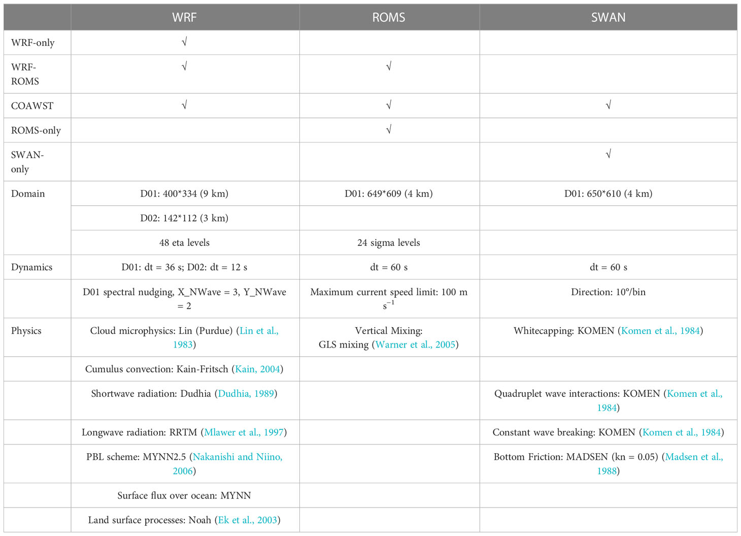
Table 1 Main experimental settings and summary of configurations across the three component models.

To further figure out the effect of waves on the surface physical process during Typhoon Megi’s passage over the SCS, another six experiments using three surface physical parameterization methods in the MYNN scheme with and without wave coupling were conducted. The newly conducted experiments with wave coupling were named C_M0, C_M1, and C_M2, while the ones without wave coupling were named WR_M0, WR_M1, and WR_M2, respectively, and the details are shown in Table 2. The parameterization methods differ in z₀, z_t, and z_q, that is, the roughness length, thermal roughness length, and moisture roughness length, respectively. M0 means the MYNN surface scheme with z₀, z_t, and z_q from the COARE algorithm, and M1 means the MYNN scheme with z₀ from Davis et al. (2008) and z_t and z_q from COARE 3.0, while M2 means the MYNN scheme with the same algorithm calculating z₀ as M1 but z_q and z_t with Garratt (1992). In this group of experiments, WR_M0 is the same as the WRF-ROMS and C_M0 is the same as the COAWST in the first group of experiments.

TABLE 2

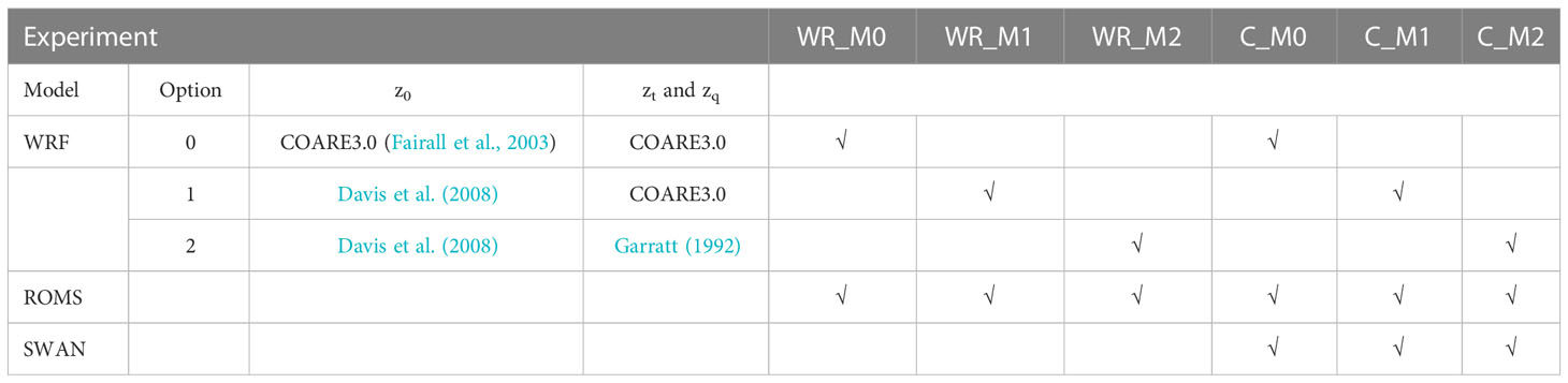
Table 2 Setting of the second group of experiments.

3 Validation of simulation results

3.1 Typhoon simulation

Super Typhoon Megi was the strongest and longest-lived TC over the NWP and SCS during 2010. Developed as a tropical depression on 13 October 2010 in the western north Pacific, Megi intensified gradually as it proceeded on a westerly course and experienced a rapid intensification from 16 to 18 October during which Megi attained its peak intensity and upgraded to a super typhoon (maximum surface wind ≥ 51.0 m s⁻¹) in the east of the Philippines. After passing through Luzon into SCS, Megi degraded dramatically to a strong typhoon at 18 UTC 18 October and headed to the northern SCS by an essentially northward track. Based on the best track data provided by CMA (Figure 1), Megi made a sharp northeastward motion at 00 UTC 20 October (Figures 2B, C). Lingering in the SCS for 5 days with a relatively slow speed of 2.0–3.5 m s⁻¹, it made landfall on the southern coast of Fujian province of China at 16 UTC 23 October.

FIGURE 2

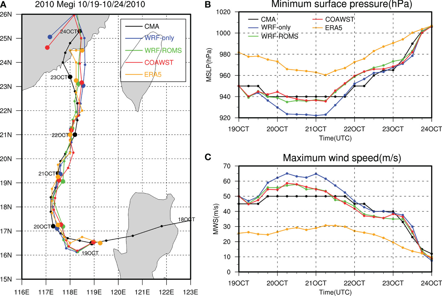
Figure 2 (A) Track of Typhoon Megi with every 6-h position, (B) the storm’s central minimum sea level pressure (hPa), and (C) the maximum sustained 10-m wind speed (m s⁻¹) from 00 UTC 19 Oct to 00 UTC 24 Oct 2010. The results based on CMA best-track data are shown in black, and the simulation results of other experiments are also shown in blue, green, and red for WRF-only, WRF-ROMS, and COAWST, respectively.

Comparison of typhoon track and intensity between the CMA best track data and the simulated results from WRF-only, WRF-ROMS, and COAWST is shown in Figure 2. Except for the first 12 h (00 UTC to 12 UTC 19 Oct), the path, structure, intensity changes, and recurvature of Super Typhoon Megi were effectively reproduced by the coupled models by using dynamic initialization and large-scale spectral nudging techniques. The simulated trajectories of Megi from WRF-only, WRF-ROMS, and COAWST are close to the CMA best track, with the mean absolute errors (MAEs) of 50.2 km, 48.2 km, and 47.7 km, respectively. The error of TC center was mainly from the turning point and the imminent landfall point, where the typhoon was affected by the complex terrain.

Although the simulated track is consistent with the observation, both the maximum 10-m wind speed (MWS) and minimum sea level pressure (MSLP) vary significantly among the WRF-only and the coupled experiments WRF-ROMS and COAWST as compared to the CMA best track data (Figures 2B, C). Since the WRF-only experiment used a prescribed SST condition from ERA5 reanalysis and thereby contained no ocean feedback, it appears that the WRF-only experiment overestimated the TC intensity during the typhoon steady state (18 UTC 19 Oct to 18 UTC 21 Oct), as compared to the CMA observation. In contrast, the WRF-ROMS and COAWST generally achieved a better typhoon intensity by using the ocean model to resolve a flow-dependent SST condition and consider the negative feedback from ocean. In the steady state of simulation, the simulated TC intensity in WRF-only is too high, while the simulated MSLP and wind speed in WRF-ROMS and COAWST is closer to the CMA observation. Overall, the MAE of TC intensity is reduced by approximately 36% compared to WRF-only.

3.2 Along-track sea surface cooling

The simulated SST of the ROMS, WRF-ROMS, and the COAWST was also checked and compared with the MW+IR OISST and HYCOM, as shown in Figure 3. Both WRF-ROMS (Figure 3D) and COAWST (Figure 3E) basically simulated the distribution of cold along-track SST observed by satellite (Figure 3A) or shown in HYCOM reanalysis (Figure 3B), though the discrepancy in magnitude is slightly big between HYCOM and simulations. Due to the weak atmospheric forcing, the simulated SST in ROMS-only is comparatively higher (Figure 3C).

FIGURE 3

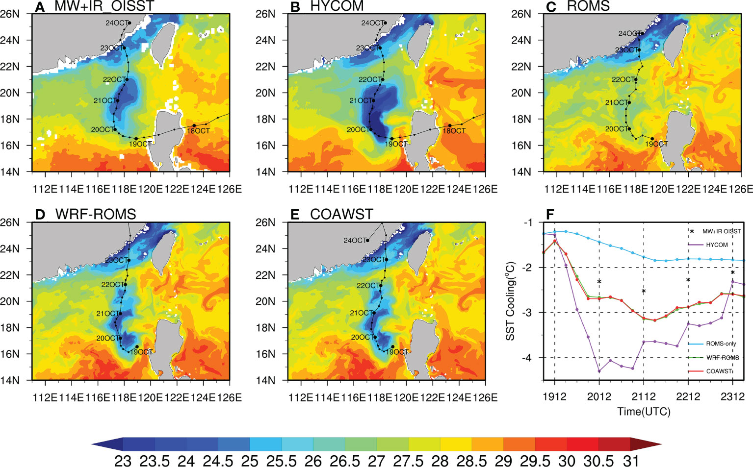
Figure 3 (A, B) Observed SST (units: °C) from MW+IR OISST, HYCOM reanalysis and (C–E) simulated SST from different experiments at 18 UTC 22 Oct. The track in (A, B) is derived from CMA best track data, (C) is derived from ERA5 reanalysis, and (D, E) is derived from its own simulation. (F) Observed and simulated average SST cooling of the cold wake. The corresponding values from MW+IR OISST are marked with black asterisks because of the daily interval of data.

Since the SST observed by satellite on the initial day (19 Oct) is approximately 2°C lower in the region of Megi’s passage than the HYCOM reanalysis, which is used for the initial field for ocean model in all experiments (figures not shown), the magnitude of SSC should be analyzed to estimate the performance of ocean response in different experiments. The range of cold wake was detected by the POLAR method (Zhang et al., 2019) from SSC. The SSC for each 6-hourly track point was defined as the SST difference between the temperature at each time spot and the temperature at the initial time, i.e., 00 UTC 19 Oct. The SSC field was firstly unified to a 0.125° resolution and converted to a polar projection centered at the TC center and azimuthally averaged with the interval of 1°. Finally, the cold wake radius was determined based on two criteria: (1) averaged SSC smaller than a threshold value of −0.7°C and (2) the radial gradient of averaged SSC< 0.1°C per 1°. After the cold wake detection, the average SSC in the cold wake area is calculated to validate the simulated cooling.

As shown in Figure 3F, compared to ROMS-only, WRF-ROMS and COAWST enhance the SSC by 60.38% and 60.36% on average, respectively. Though the SSC is 0.5°C greater than satellite observation due to the stronger simulated surface wind, it is still acceptable. It is significant that the HYCOM reanalysis overestimated the SSC, including the magnitude, and the time when maximum cooling occurs. This may be related to the lack of tidal forcing in the HYCOM reanalysis (Cao et al., 2021), which may result in stronger near-inertial waves, which, in turn, increases turbulent mixing (Guan et al., 2014).

In summary, discrepancies exist between the simulated results and observed data, but the coupled experiments WRF-ROMS and COAWST show good consistency with both observations and reanalysis data after Megi entered the SCS, especially during the most intense stage.

3.3 Thermal response

To further understand the effects on the upper ocean thermal and dynamical responses during Typhoon Megi, the ocean temperature and salinity profile, ocean currents, and the changes in ocean mixed layer depth (MLD) were checked and compared with the in-situ observations.

The temperature and salinity profile of four Argo floats (A1–A4), as introduced previously, were plotted and compared in the upper 1,000 m depth in Figures 4A–H. The figure shows that all three experiments can simulate the vertical distribution of ocean temperature and salinity well and with slight difference, especially where the vertical temperature gradient is large, that is, at the MLD. The two Argo floats, A2 and A3, are located on the TC track and most affected by the typhoon obviously, followed by A1. In the upper ocean at depths of 0–300 m, the MAE of temperature was reduced by 47%, 81%, and 51% in WRF-ROMS and 40%, 83%, and 47% in COAWST for A1, A2, and A3, compared to ROMS-only, respectively. As A4 is far away from the TC track, the results in different experiments are similar, indicating that it is almost unaffected by the typhoon. The good performance of coupled experiments demonstrates the effectiveness in thermohaline structure simulation.

FIGURE 4

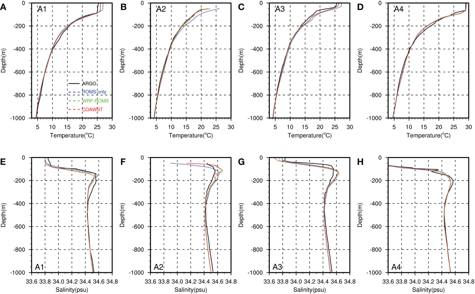
Figure 4 Comparison of temperature profile (top) and salinity profile (bottom) between observation and simulation at each position of Argo floats A1 (A, E), A2 (B, F), A3 (C, G) and A4 (D, H).

Besides Argo float records, the observations of two moorings located to the left and right sides of the TC center at 00 UTC 22 Oct were also examined to verify the effectiveness of ocean state simulation. Figure 5 shows the upper ocean thermal structure evolving captured by mooring R1. The upper layer was warm and thick before the intrusion of Typhoon Megi, with the 26°C isothermal line at approximately 80 m depth (Figure 5A), suggesting the fore-eye warming in the open sea. After the passage of Typhoon Megi, the rapid rise of isothermal lines up to 50 m toward the sea surface occurred nearly the entire observed water column (from 60 to 360 m; Figure 5A), indicating a strong Ekman-pumped upwelling due to the relatively slow movement of Megi in SCS (Price, 1981; Guan et al., 2014). This phenomenon is better captured by WRF-ROMS and COAWST (Figures 5C, D), as the shallowing of the temperature mixed layer and the uplifting of the thermocline were qualitatively depicted in both coupled experiments, while the ROMS-only simulated moderate cooling in the upper layer (Figure 5B).

FIGURE 5

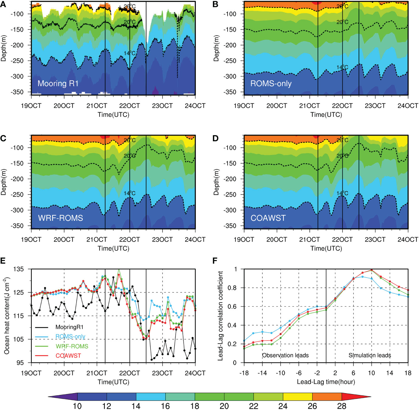
Figure 5 (A–D) Comparison of contours of temperature versus time and depth between (A) Mooring R1 and simulation (B) ROMS-only, (C) WRF-ROMS, and (D) COAWST at the position of mooring R1. The 14, 20, and 26°C isothermal lines are plotted and labeled. (E) Ocean heat content (units: J cm⁻²) integrate between 60 m and 200 m at the position of mooring R1. (F) Lead-Lag correlation coefficient between experiments and the observation. Vertical lines in (A–E) indicate the times during Megi’s approaching, arriving, and passing over.

With the colder thermocline water lifted up, the upper ocean heat content (OHC) decreased. To verify the simulation of this process in each experiment, the OHC from 60 m to 200 m was estimated via the following equation:

$\begin{array}{ll}OHC={\rho }_0{C}_{\rho }{\displaystyle {\int }_{200}^{60}T(z)dz}& (1)\end{array}$

Where ρ₀ = 1,024 kg m^-3 is the reference water density and C_ρ = 4,000 J k°C^-1 is the heat capacity.

Figure 5E compares the OHC between observation by mooring R1 and the simulations of three experiments. Both observation and simulation can capture the variation of OHC though it is higher in simulations. As Typhoon Megi approaches, there is a slight increase. When Megi arrived, the strong wind near the inner core of TC leads to the sudden cooling of the upper ocean. Comparing the pre-typhoon (mean value from 00 UTC 19 Oct to 06 UTC 21 Oct) and post-typhoon (mean value of the lowest points) OHC at the position of R1, after the passage of Megi, the estimated OHC decreased by 17% from 119.6 J cm⁻² to 99.2 J cm⁻² in observation; in ROMS-only, it decreased by 9.7% from 126 J cm⁻² to 113.8 J cm⁻²; in WRF-ROMS, it decreased by 16% from to 126.2 J cm⁻² to 106 J cm⁻²; and in COAWST, it decreased by 16.3% from 126.1 J cm⁻² to 105.6 J cm⁻². Both WRF-ROMS and COAWST simulated the decrease rate of OHC well but COAWST is better, and the underestimated decrease of OHC in ROMS-only is similar to the weak variation of isotherms due to the weak wind forcing.

The cooling process in observation lags behind that in simulations. To explore the similarity between the observed OHC and simulated OHC in trend, the lead-lag correlation is calculated in Figure 5F. The peaks show that observation lagged ROMS-only by approximately 8 h, and WRF-ROMS and COAWST by approximately 10 h, probably because the simulated typhoon was moving a little faster as it passed over the mooring R1 than the actual typhoon did (Figure 2A), and the thermal response may appear earlier. Moreover, the response to wind stress in the upper ocean below the mixed layer may also be delayed in actual conditions.

The mixed layer is critical for air–sea interaction and oceanic dynamic processes, particularly in the tropics. The MLD was shallower after the passage of Megi, but could be barely estimated through mooring R1 observation accurately, because the temperature difference between the surface and the top of the temperature chain (65 m) was unmeasured. However, it can be captured by the records from Argo floats (Figures 4A–D), and under the impact of typhoon, the MLD at A1 (approximately 60 m), A2 (approximately 50 m), and A3 (approximately 40 m) is relatively shallower than that at A4 (approximately 75 m).

The simulation also supports the observed shallower mixed layer by Argo floats after the typhoon passed. Figure 6 compares the simulated density MLD determined by a new hybrid method proposed in Holte and Talley (2009) at 00 UTC 22 October 2010. Although some differences exist between the ROMS-only, WRF-ROMS, and COAWST, it is clear that the density MLD becomes shallower in the area after the passage of Typhoon Megi. Figure 6D shows the time variation of average MLD in the inner core of the TC center at 00 UTC 22 Oct. The MLD in three experiments varied moderately when Typhoon Megi approached; all quickly increased from near 30 dbar to approximately 45 dbar. Then, the simulated MLD gradually decreased when Typhoon Megi arrived and passed by. Due to the thin mixed layer in the northern SCS and strong thermocline, the uniform upper layer was susceptible. With the strong wind in the TC forcing stage, the shallowing mixed layer was led by the active entrainment near the bottom of the mixing layer, accounting for the sharp vertical temperature or salinity shear near the sea surface. The less shallowing mixed layer and weakest MLD variation simulated by ROMS-only may indicate the impacts of strong cyclonic wind near the sea surface.

FIGURE 6

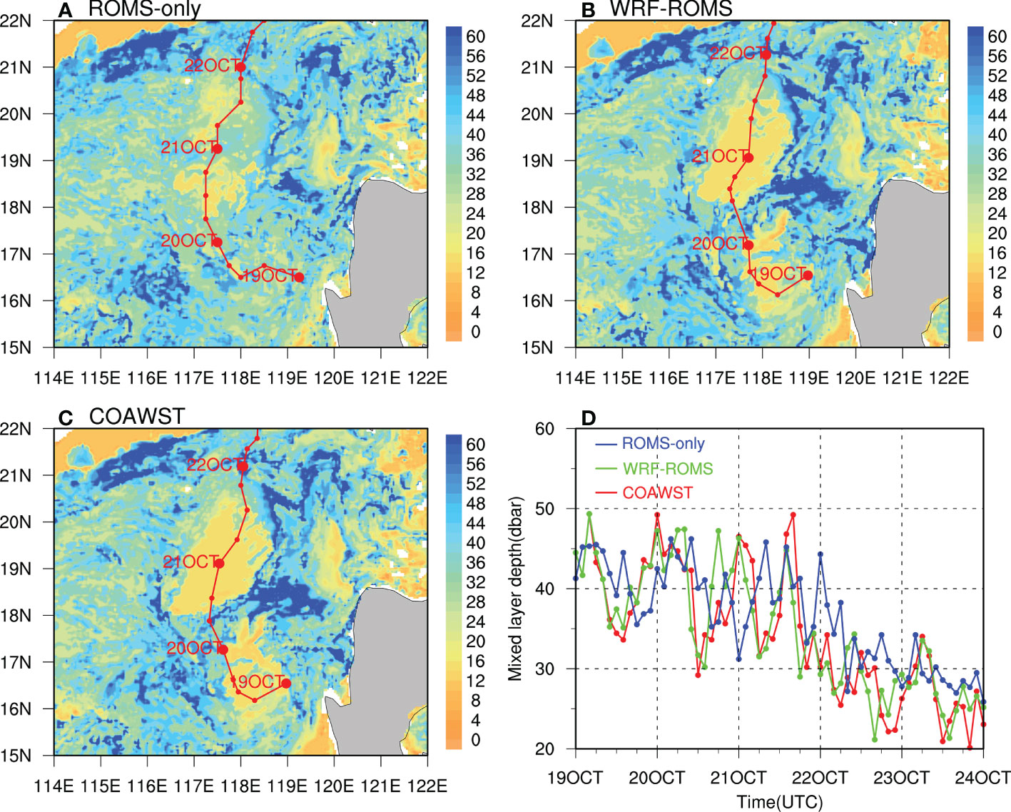
Figure 6 Simulated density mixed layer depth (dbar) of experiments at 00 UTC 22 Oct for (A) ROMS-only, (B) WRF-ROMS, and (C) COAWST. The track (solid red line) in (A) is derived from ERA5 reanalysis, (B) is from WRF-ROMS simulation, and (C) is from COAWST simulation. (D) Comparison of the changes of density mixed layer depth, the average value in the region 50–150 km away from the TC center at 00 UTC 22 Oct (21.0°N,118.2°E).

3.4 Current response

The observed and simulated upper ocean current response at mooring L1 and mooring R1 are presented in Figure 7. Before Megi’s arrival, the background current was strong (up to 0.8–1 m s⁻¹ at L1 and 0.6–0.9 m s⁻¹ at R1), consisting of signals from the ocean environment, especially the strong internal tides (Figures 7A, E). After the passage of Megi, significant momentum was injected into the ocean, and the raw current velocity increased immediately at both moorings (mainly above the 100-m depth, and more consistent above 80 m). Notably, near 12 UTC 21 Oct and 06 UTC 22 Oct during the passage of Megi, the increase in northwest velocity was followed by the rise of isotherms at R1. The oscillations of the isotherms may be driven by the divergence and convergence of inertial current, which would induce subsurface water cooling and warming. Some features captured by model simulation are less obvious in the observations. All experiments showed the characteristics of near-inertial oscillations (NIOs), i.e., an increase in energy in the near-inertial period. Moreover, the observed current in the upper level was out of phase with that at deeper levels in observation, indicating the baroclinic response related to NIOs, while the results of experiments are more barotropic. However, the typhoon-generated near-inertial currents were masked in the strong background flow.

FIGURE 7

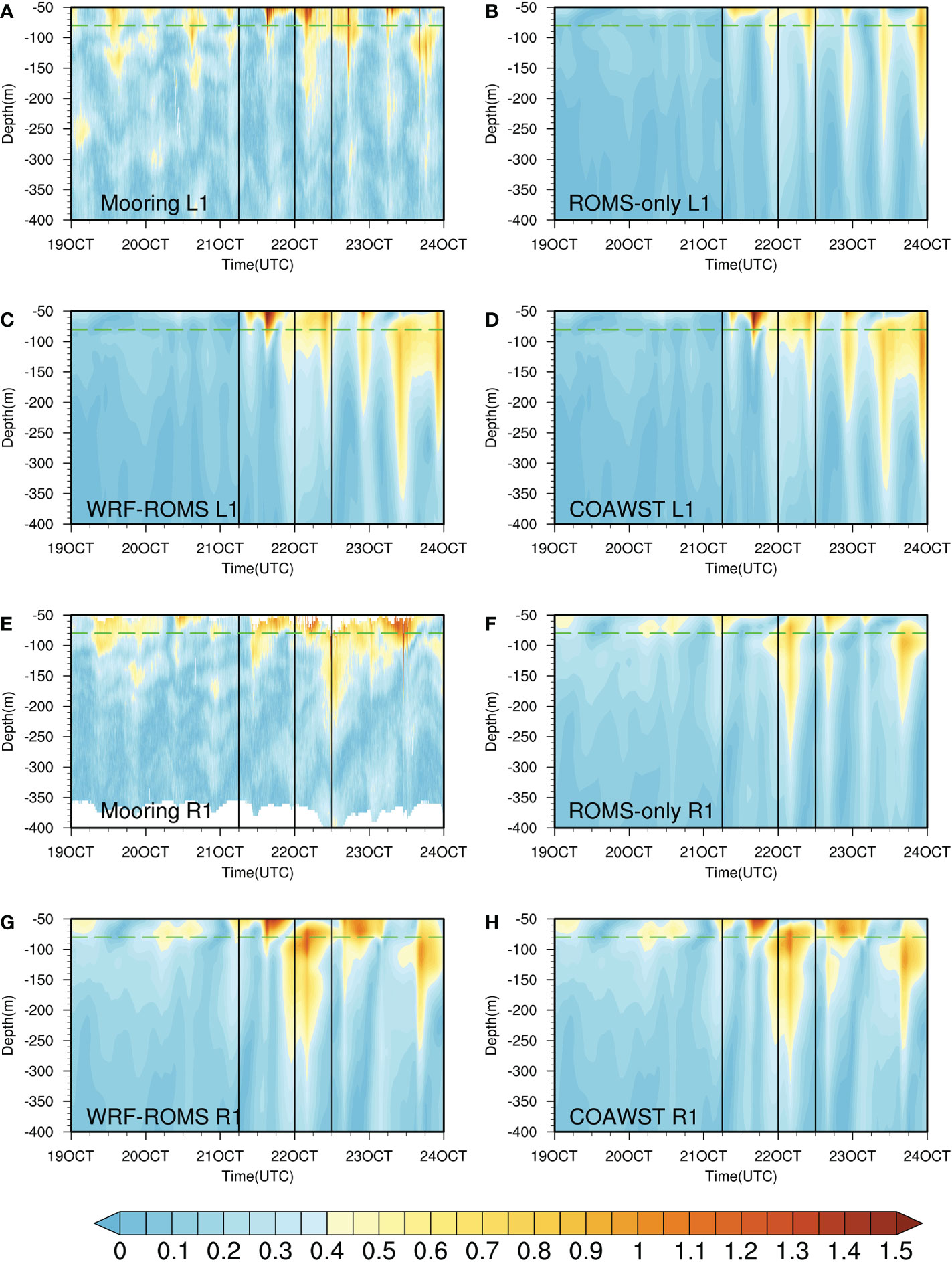
Figure 7 Comparison of contours of raw current velocity between observation and simulation at the position of (A–D) mooring L1 and (E–H) mooring R1 versus time and depth. Vertical lines indicate the times during Megi’s approaching, arriving, and passing over.

Figures 8A, B show the 50–80 m average current, and it is mainly northwestward, which was consistent with the direction of the internal wave propagation from the Luzon Strait to the SCS. The current speed is stronger at R1 in general, indicating the right-biased intense currents, which may be caused by the resonance effect of the wind stress on the right side of the track. The clockwise-rotating motion of current speed that decayed slowly with time in observation was also well simulated in all experiments.

FIGURE 8

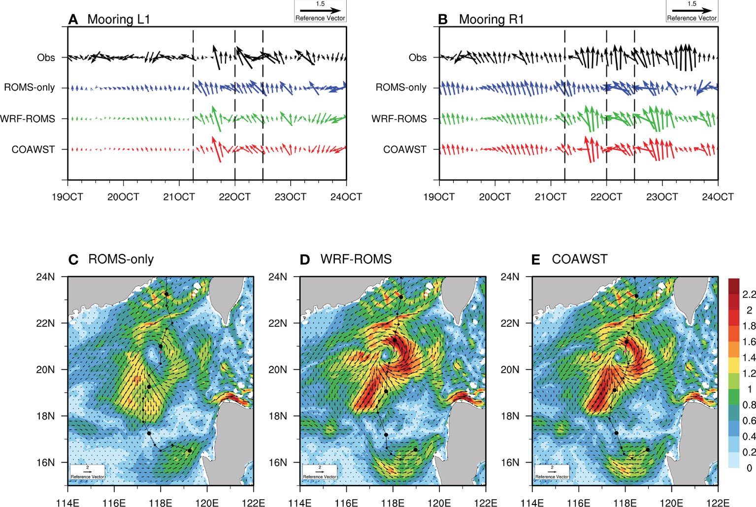
Figure 8 (A, B) Comparison of ocean current direction at mooring L1 and R1 in the upper ocean (50–80 m) averaged. Vertical dashed lines indicate the times during Megi’s approaching, arriving, and passing over. (C–E) Comparison of simulated ocean currents of ROMS-only (C), WRF-ROMS (D), and COAWST (E) at 18 UTC 21 Oct. The track information is the same as Figure 3, and the tropical cyclone center at this time is marked with magenta dots.

As Typhoon Megi moves over the ocean, the wind stress caused by strong surface wind induces the adjustment of ocean currents to flow in the direction of the wind, and the current speed increased (Figures 8C–E). After the passage of the TC, the current on the left side of the track rotates clockwise as the wind stress changes, and the atypical left bias may be related to the topography, as the northern reaches are over the steep continental slope, of which the topographic beta effect could shift the ocean current westward as a whole (Ko et al., 2014). Note that the current speed in COAWST is weaker than that in WRF-ROMS, indicating the effect of wave–current interaction. With weak wind forcing, the surface current distribution is also different, not only in the magnitude of current speed, demonstrating the complex interaction between wind, current, and wave.

3.5 Surface waves

The generation and growth of surface waves are the effects of surface wind. At the same time, the wave state could modify the current structure on both sides of the air–sea interface (Liu et al., 2012). In this subsection, we validate and discuss the simulated wave results in terms of significant wave height (H_s).

Figures 9A–C demonstrate the comparison between the significant wave height (H_s) at 00 UTC 22 Oct in ERA5 reanalysis and the simulation of COAWST and SWAN-only. Both COAWST and SWAN-only simulated the observed largest H_s in the continental slope and shelf regions (Figure 1) due to the piled-up effect. However, in terms of the magnitude, the maximum H_s of SWAN alone is 8.56 m, compared with 10.78 m in ERA5 reanalysis and 11.58 m in COAWST. The H_s on the right side of TC track in COAWST is higher because of the stronger wind than SWAN-only and ERA5. Figure 9D shows the change of high H_s with time to the left side of TC center at 00 UTC 22 Oct. The variations all show the maximum H_s when TC approached at 12 UTC 21 Oct, ahead of the arrival, which may be related to the wave–current interaction and piled-up effect. The difference in magnitude of H_s between COAWST and SWAN-only shows the effectiveness in the fully coupled model.

FIGURE 9

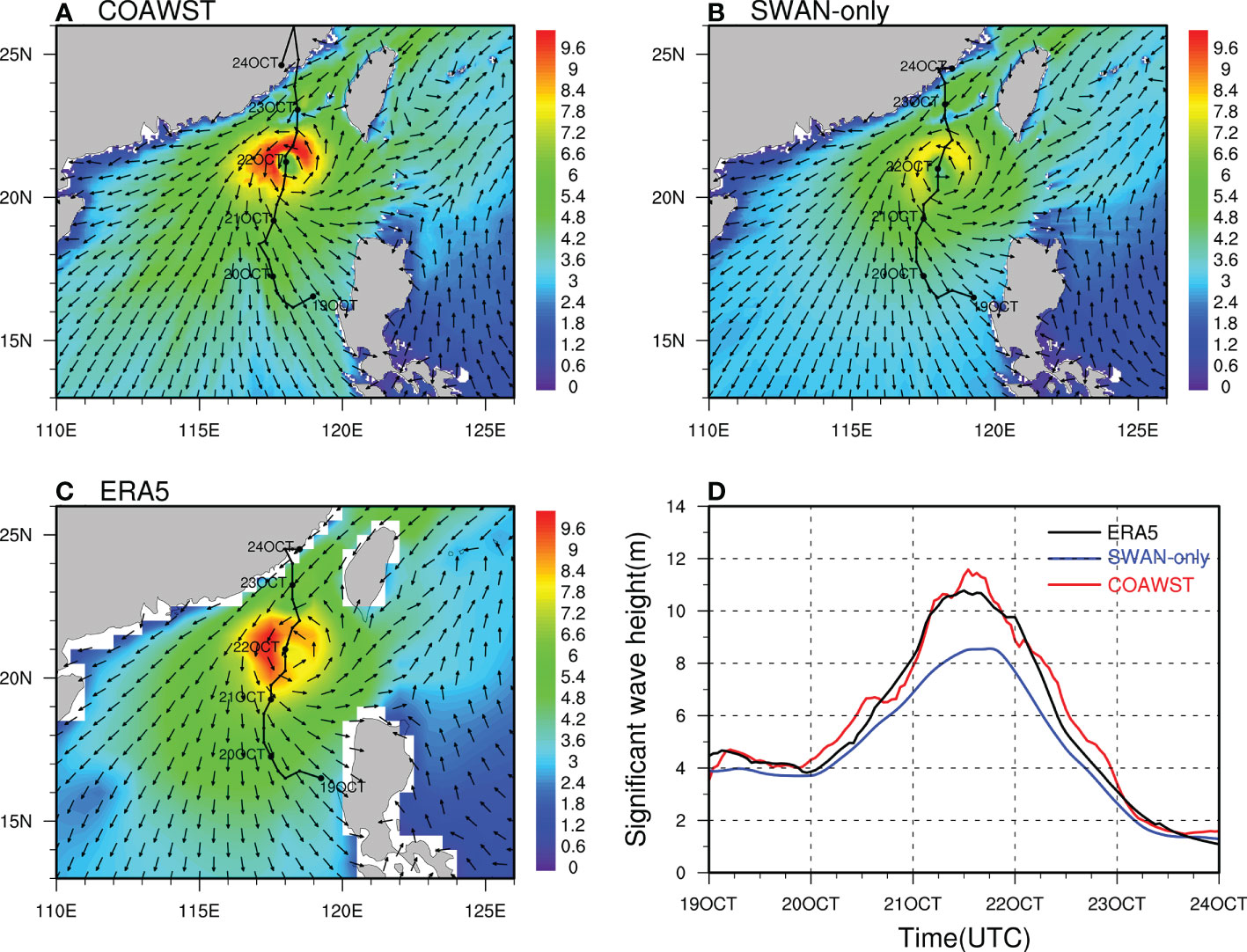
Figure 9 Comparison of significant wave height (shaded, units: m) and wave propagation direction (vector) between simulations of (A) COAWST, (B) SWAN-only, and (C) ERA5 reanalysis at 00 UTC on 22 October. The track (solid black line) in (A) is derived from COAWST simulation, and (B, C) is derived from ERA5 reanalysis. (D) Comparison of the changes of significant wave height (H_s), the average value in the region with high H_s (larger than 7.8m in A) to the left side of TC center at 00 UTC 22 Oct.

4 Wave effects

4.1 The uncertainty of wave effects on TC intensity

The results shown in Section 3 suggested the importance of using the atmosphere–ocean coupled model in simulating the typhoon, but the effects of coupling waves on typhoon simulation are uncertain and remain to be further explored. As shown in Figure 9, it was found that in the COAWST model, wind forcing did play a significant role assisting the growth of waves. Here is an interesting question: Why did the COAWST experiment seem to have simulated a similar intensity of Typhoon Megi to WRF-ROMS, as well as ocean currents and thermal structure in the upper ocean during the passage of the typhoon? According to previous studies (Holthuijsen et al., 2012; Liu et al., 2012; Chen et al., 2013), there are mainly two opposite effects of waves. The first is that the growth of waves will increase the sea surface roughness, thereby increasing the wind stress and transmitting more momentum fluxes into the ocean. On the other hand, the generation of sea sprays at the air–sea interface induced by wave breaking could have a positive effect on typhoon intensity by releasing latent heat and sensible heat extracted from the warmer ocean. This inspires us that the difference between the experiments with and without wave coupling may be more obvious in surface physical process.

Considering that the wave affects the typhoon intensity mainly by modifying the heat and momentum exchange between air and sea, we further compared several important sea surface physical processes under Typhoon Megi, including 10-m wind speed, surface wind stress (also known as the momentum flux), latent heat flux, and sensible heat flux in Figure 10.

FIGURE 10

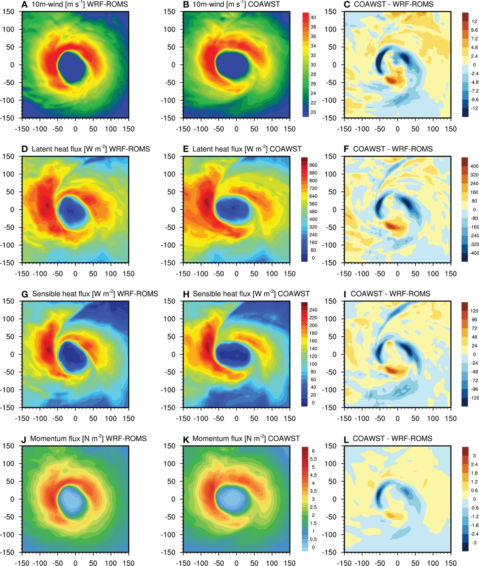
Figure 10 The simulated 10-m wind speed (A–C), latent heat fluxes (D–F), sensible heat fluxes (G–I), and momentum fluxes (J–L) from experiment WRF-ROMS, COAWST, and their difference at 00 UTC 22 Oct.

As shown in Figures 10A, B, the higher wind speed in WRF-ROMS than in COAWST can reach 12 m s⁻¹ near the RMW (radius of maximum surface wind), and the simulated inner core structure of Typhoon Megi was different in the two experiments. The structure was more axisymmetric in the WRF-ROMS, resulting in larger and more concentrated latent heat flux and sensible heat flux in the eyewall region. The energy was therefore more efficiently collected and assisted the development of Typhoon Megi, leading to stronger wind speed. However, the momentum flux, determined by the surface wind speed and the wave-affected sea surface roughness, had an opposite effect, transporting the energy from the typhoon to the ocean below. It could offset the increased heat flux and therefore weaken the maximum wind speed in WRF-ROMS to the intensity of that in COAWST, with the small difference of approximately 1 m s⁻¹ (Figure 2C). Overall, the TC intensity is the result of the balance of heat and momentum obtained and lost. It implies that the effect of waves should be taken into consideration when conducting atmosphere–ocean coupling simulations, but the surface flux parameterization scheme should be chosen carefully due to the uncertainty of the wave effect on the surface physical process.

4.2 The wave effects on surface fluxes

According to previous works (Taylor and Yelland, 2001; Oost et al., 2002; Drennan et al., 2005), there are different combinations of sea surface physical parameterization schemes in describing the effects of surface waves. The problem of whether and how different parameterization schemes affect the TC-induced ocean state needs to be investigated carefully. To figure out the effects of different combinations of estimations for surface momentum flux and heat flux when coupling waves, we further conducted an additional six experiments using different surface physical parameterization methods in the MYNN scheme with and without wave coupling. The newly conducted experiments with wave coupling were named C_M0, C_M1, and C_M2, while the ones without wave coupling were named WR_M0, WR_M1, and WR_M2, respectively. WR_M0 is the same as the WRF-ROMS and C_M0 is the same as the COAWST in the first group of experiments.

As mentioned above, the wave effect mainly acts on the inner core region of the typhoon. To avoid the smoothing effect caused by averaging, the changes between radii that are 0.5 and 3.0 times that of RMW are emphasized (Figure 11). Though the maximum wind speed of Typhoon Megi (2010) was similar in WR_M0 and C_M0 at 18 UTC 19 Oct and 12 UTC 20 Oct (Figure 2C), the azimuthally averaged peak surface wind speed at RMW was slightly weaker in C_M0 than in WR_M0 (Figure 11A), indicating the negative effects of waves by increasing the sea surface roughness during the simulations.

FIGURE 11

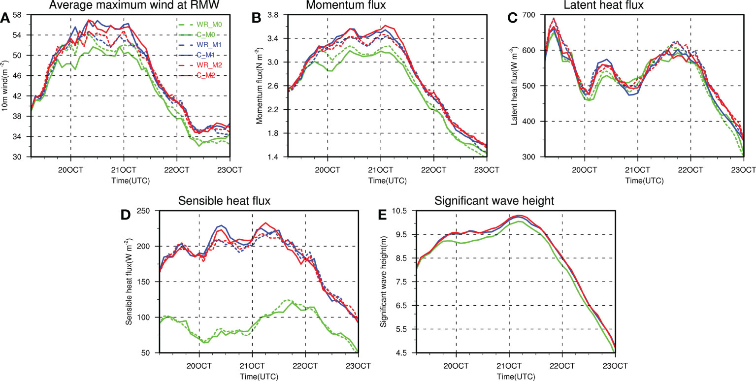
Figure 11 Time series of simulated (A) azimuthally averaged peak surface wind speed at the radius of maximum wind (RMW), (B) momentum fluxes, (C) latent heat fluxes, (D) sensible heat fluxes, and (E) significant wave height averaged over an annular area between radii of 0.5 and 3.0 times of RMW from 06 UTC 19 Oct to 00 UTC 23 Oct (M0—green, M1—blue, and M2—red). The solid lines denote the fully coupled experiments while the dashed lines show the results of the no-wave effects results.

Using the COARE algorithm, WR_M0 and C_M0 had a significantly weaker typhoon intensity and momentum flux than the other two sets in Figures 11A, B, and it is also demonstrated by the significant wave height forced by surface wind (Figure 11E). However, different from previous studies (Warner et al., 2010), C_M1 and C_M2 simulated an azimuthal mean wind speed of approximately 4 m s⁻¹ stronger than WR_M1 and WR_M2, accompanied by a moderately stronger momentum flux (Figure 11B). Since the z₀ was calculated following Davis et al. (2008) in both M1 and M2 experiments, the wind stress was also similar in these experiments.

With the same z_t and z_q schemes, the surface heat fluxes differ in M0 and M1 experiments, while the heat fluxes in M1 are more similar to M2 with different z_t and z_q schemes, because the wave-modified sea surface roughness (z₀) not only impacts the amount of momentum flux transferred into water columns but also determines the heat-flux exchange coefficients together with z_t and z_q (Liu et al., 2014). As shown in Figures 11C, D, both latent heat flux and sensible heat flux were higher in C_M1 and C_M2, supporting the corresponding stronger typhoon intensity. Since the contribution of sea sprays to the heat flux is amplified, the total heat flux, especially the sensible heat flux, was evidently enhanced by the waves. In contrast, C_M0 simulated about half the amount of the sensible heat flux, and the wave effect shows the least impact on the heat flux compared to the other two sets, though a better typhoon intensity was simulated with this combination of parameterization schemes.

Through the above discussions, the wave was proved to impact both momentum flux and enthalpy flux during the typhoon simulations, including the positive effect on the typhoon through enhanced heat flux and the negative effect through the momentum flux transported into the ocean. This may be the reason why the results from the two experiments COAWST and WRF-ROMS were similar. In addition, the characteristics at the air–sea surface could be significantly determined by the surface physical parameterization option because of the different implementations of the wave effects during the numerical simulation.

4.3 The wave effects on thermal response

The ocean temperature in the upper 200 m affected by Typhoon Megi in the experiments is also compared in Figure 12. Under the influence of strong winds, there is a rapid rise in isothermal lines of up to 50–60 m toward the sea surface. With z₀ calculated following Davis et al. (2008), the surface wind is much stronger in M1 and M2 than in M0 (Figure 11A), inducing stronger Ekman pumping, and the depth of the 22°C isotherm line can be up to 45 m. After the passage of Megi, the estimated OHC (calculated by Equation 1) decreased by 16.7% in WR_M0, 18.6% in C_M0, 17.9% in WR_M1, 20.2% in C_M1, 18.9% in WR_M2, and 19.7% in C_M2. Note that the difference between C_M1 and WR_M1 is larger than that between the other two sets, suggesting that the wave effect varies greatly under different surface physical parameterization schemes. From 00 UTC 20 Oct to 06 UTC 21 Oct, during Megi’s approach, arrival, and passage, the surface wind is approximately 4 m s⁻¹ stronger in C_M1 and C_M2 than in WR_M1 and WR_M2 (Figure 11A), accounting for the stronger Ekman-pumped upwelling in experiments with wave coupling (Figures 12D, F).

FIGURE 12

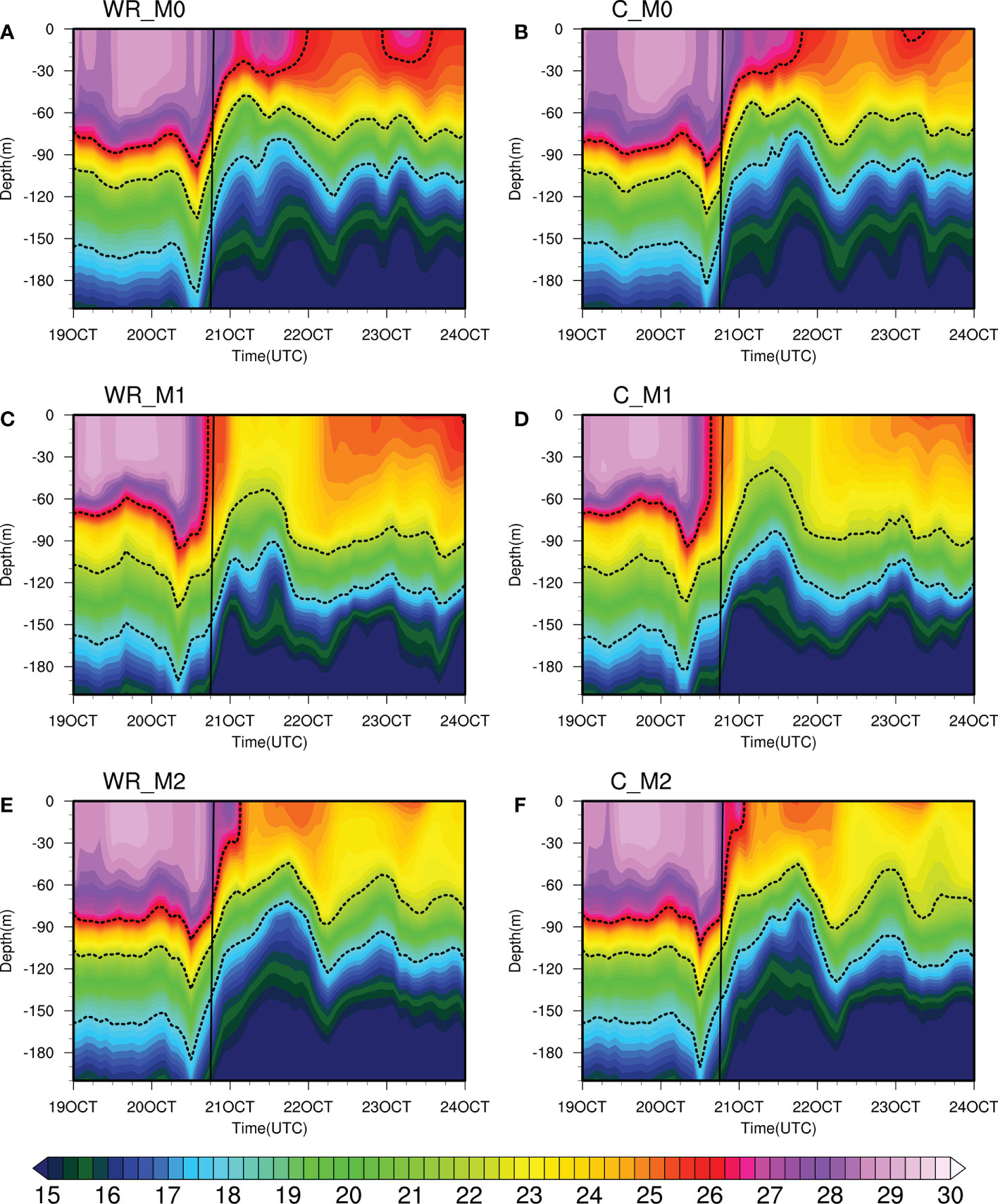
Figure 12 The simulated temperature variation azimuthally averaged at the RMW on the right side of TC center at 18 UTC 20 Oct versus time and depth in (A) WR_M0, (B) C_M0, (C) WR_M1, (D) C_M1, (E) WR_M2, and (F) C_M2. The vertical line indicates the time during Megi’s arriving. The three black isolines represent the 26, 22, and 18°C isothermal lines from top to bottom, respectively.

Though the surface wind is weaker in C_M0 than that in WR_M0, the temperature is approximately 1°C colder from 0 to 50 m in the upper layer in C_M0 than that in WR_M0 after Megi’s passage, indicating the vertical mixing induced by wave rather than the stronger winds. Since wave breaking is not considered in our simulation, the nonbreaking wave-stirring-induced vertical mixing may be the main process of the enhanced vertical mixing, which can transfer kinetic energy from surface waves to ocean circulation through the processes of vertical wave motion and the wave-induced Reynolds stress, especially in the SCS (Li et al., 2014).

After 00 UTC 22 Oct, the isotherms still oscillated, indicating the subsurface water cooling and warming, and the amplitude of oscillation is also different, especially between M1 and M2. Though the same algorithm was used for z₀ in these two sets of experiments, the thermal response induced by the typhoon is still different. This implies that the upper ocean response may also be sensitive to surface physical parameterization.

5 Conclusions and discussion

To explore the effects of ocean states coupling on the simulated Super Typhoon Megi in the SCS and further understand the ocean feedbacks to super typhoons, five sensitive experiments using WRF-only, ROMS-only, SWAN-only, coupled WRF-ROMS, and fully coupled WRF-ROMS-SWAN model, separately, were designed and analyzed. Simulation results were validated and evaluated against observations. Results suggest that the simulated TC track is insensitive to ocean feedbacks, and ocean states coupling could moderately improve the simulation of intensity with the MAE of the TC intensity reduced by 36% in coupled models, compared with that in the WRF-only experiment.

As presented in the above sections, all experiments, ROMS-only, WRF-ROMS, and COAWST, show time consistency of the ocean response with satellite data and in-situ observations during Typhoon Megi, indicating the effectiveness of the simulation. However, only WRF-ROMS and COAWST show favorable comparison in magnitude with observations. The SST cooling and OHC were checked and proved to be heavily dependent on the strong wind stress on the sea surface. Since subsurface OHC has also been suggested to be potentially influential for TC genesis (Huang et al., 2015), accurate prediction of ocean state in the complex SCS is important for the subsequent forecast of TC generation during the typhoon season. The result highlights the importance of reliable atmospheric forcing for ocean models.

Supported by the observations and simulations, the mixed layer became shallower after Typhoon Megi passed, and it was led by the active entrainment near the bottom of the mixing layer. The NIOs could also be captured in both surface ocean currents and subsurface isotherm, indicating the baroclinic ocean responses during the passage of Typhoon Megi. The surface currents are weaker than WRF-ROMS when coupling waves in the COAWST experiment, indicating the role of wave–current interaction. The significant wave height (H_s) shows left-biased strengthening, which may be related to the appearance of the continental shelf and to the time when H_s reached the maximum ahead of the typhoon arrival.

Results in both atmosphere and ocean are similar between the WRF-ROMS and COAWST experiments. This seems to lead to a conclusion that the ocean state was less obvious when wave was coupled in the air–sea coupled model. However, further analysis showed that the wave impacted both dynamical and thermal processes near the sea surface prominently. The wave was proved to have a negative effect on the typhoon through reduced heat flux but a positive effect through the correspondingly decreased momentum flux transported into the ocean. This may be the reason why results from the two experiments that were similar to the effect of wave coupling on typhoon intensity were covered up. Since a large amount of heat and momentum exchange at the air–sea interface could have opposite effects on typhoon intensity, the uncertainty of coupling waves for typhoon simulation needs to be further explored.

Six experiments using three surface physical parameterization methods in the MYNN scheme with and without wave coupling were conducted to further figure out the wave effects on typhoon and eliminate the contingency brought by the surface parameterization scheme. The effect of waves on typhoon intensity was not unique, as the surface wind was stronger with wave coupling in C_M1 and C_M2, and weaker in C_M0. With different combinations of estimations for surface momentum flux and heat flux, the simulated surface wind and surface fluxes in M0 experiments differ a lot from the other two sets, M1 and M2, indicating the uncertainty of the wave effect on the surface physical process and the crucial impact of surface physical parameterization options during simulations. Overall, the TC intensity is determined by the net surface flux. Furthermore, the additional ocean cooling induced by weaker surface wind than WR_M0 after Megi’s passage in C_M0 also demonstrates the role of nonbreaking wave-stirring-induced vertical mixing, indicating that the wave feedback does exist in the fully atmosphere–ocean–wave coupled model.

The relative importance of wave effects, including the changes to sea surface roughness, enhanced vertical mixing, and the increased heat flux to typhoon due to the generation of sea sprays, is well worth studying. Because of the barren sea surface observations during strong typhoons, whether the wave effect plays a positive role, enhancing the enthalpy flux, or a negative role, weakening the wind through the rougher sea surface, was hard to verify. However, one should note the complexities and the contributions of the wave effects when developing the coupled models. According to Xu et al. (2022), a more advanced sea spray parameterization scheme could help to improve the effects of coupling waves evidently in the coupled atmosphere–ocean–wave model, it is also a challenging work in the future.

It is shown that ocean states coupling can improve typhoon simulation, but how the wave impacts typhoon intensity remains uncertain. Our findings highlight the importance of accurate initial wind forcing field, model configurations, and surface physical process parameterization in TC simulations with the coupled model, especially when coupling waves. Moreover, as the ocean feedback during the TC passage is essential to reproduce the atmospheric and ocean state realistically, and the realistic three-dimensional typhoon–ocean system is extremely complex, the optimal combination of components of this complex system is hard to estimate and full of uncertainty. The quantitative estimations of the impact of different model combinations and surface physical parameterization combinations on simulating Typhoon Megi, especially in the highly complex SCS, could provide a reference for model selection in similar cases.

Data availability statement

The CMA best-track data were obtained from https://tcdata.typhoon.org.cn/en/zjljsjj_sm.html. The MW+IR OISST product were retrieved from https://www.remss.com/measurements/sea-surface-temperature/oisst-description/. The HYCOM reanalysis were downloaded from https://www.hycom.org/data/glbv0pt08/expt-53ptx and https://www.hycom.org/data/glbu0pt08/expt-19pt1. The ERA5 reanalysis data were retrieved from https://www.ecmwf.int/en/forecasts/datasets/reanalysis-datasets/era5. The Argo float profiles were available at http://www.argo.org.cn/. The topographic data ETOPO2 were obtained from https://sos.noaa.gov/catalog/datasets/etopo2-topography-and-bathymetry-natural-colors/. The TPXO tidal data were retrieved from http://g.hyyb.org/archive/Tide/TPXO/TPXO_WEB/global.html.

Author contributions

ZZ and WZ: conceptualization. HW: data curation. MZ, MF and ZZ: methodology and modeling. MZ and MF: analysis and visualization. MZ and ZZ: writing—review. WZ: supervision. All authors contributed to the article and approved the submitted version.

Funding

This research was jointly funded by the National Key R&D Plan Program of China (2021YFC3101500) and the National Natural Science Foundation of China (Key Program, No. 41830964).

Acknowledgments

We would like to thank Jiwei Tian for providing the processed mooring data used to construct figures in this work, and the Remote Sensing Systems (http://www.remss.com) for providing the MW + IR OI SST product. Besides, the authors would like to thank Dr. Yineng Li and Jae-Hyoung Park for their helpful review comments and the draft sorting from Rui Chen.

Conflict of interest

The authors declare that the research was conducted in the absence of any commercial or financial relationships that could be construed as a potential conflict of interest.

Publisher’s note

All claims expressed in this article are solely those of the authors and do not necessarily represent those of their affiliated organizations, or those of the publisher, the editors and the reviewers. Any product that may be evaluated in this article, or claim that may be made by its manufacturer, is not guaranteed or endorsed by the publisher.

References

Booij N., Ris R. C., Holthuijsen L. (1999). A third-generation wave model for coastal regions: 1. model description and validation. J. Geophys. Res. 104 (C4), 7649–7666. doi: 10.1029/98JC02622

CrossRef Full Text | Google Scholar

Cao A., Guo Z., Pan Y., Song J., He H., Li P. (2021). Near-inertial waves induced by typhoon Megi, (2010) in the south China Sea. J. Mar. Sci. Eng. 9 (4), 440. doi: 10.3390/jmse9040440

CrossRef Full Text | Google Scholar

Chen X., Pan D., He X., Bai Y., Wang D. (2012). Upper ocean responses to category 5 typhoon megi in the western north pacific. Acta Oceanol. Sin. 31, 51–58. doi: 10.1007/s13131-012-0175-2

CrossRef Full Text | Google Scholar

Chen S., Zhao W., Donelan M., Tolman H. (2013). Directional wind–wave coupling in fully coupled atmosphere–Wave–Ocean models: Results from CBLAST-hurricane. J. Atmos. Sci. 70 (10), 3198–3215. doi: 10.1175/JAS-D-12-0157.1

CrossRef Full Text | Google Scholar

Chu P., Veneziano J., Fan C., Carron M., Liu W. (2000). Response of the south China Sea to tropical cyclone Ernie 1996. J. Geophys. Res. 105 (C6), 13991–14009. doi: 10.1029/2000JC900035

CrossRef Full Text | Google Scholar

D’Asaro E., Black P., Centurioni L., Harr P., Jayne S., Lin I.-I., et al. (2011). Typhoon-ocean interaction in the western north pacific: Part 1. Oceanography 24 (4), 24–31. doi: 10.5670/oceanog.2011.91

CrossRef Full Text | Google Scholar

Davis C., Low-Nam S. (2001) The NCAR-AFWA tropical cyclone bogussing scheme. a report prepared for the air force weather agency (AFWA). Available at: http://www.mmm.ucar.edu/mm5/mm5v3/tc-bogus.html.

Google Scholar

Davis C., Wang W., Chen S., Chen Y., Corbosiero K., DeMaria M., et al. (2008). Prediction of landfalling hurricanes with the advanced hurricane WRF model. Mon. Wea. Rev. 136, 1990–2005. doi: 10.1175/2007MWR2085.1

CrossRef Full Text | Google Scholar

Drennan W., Taylor P., Yelland M. (2005). Parameterizing the Sea surface roughness. J. Phys. Oceanogr. 35 (5), 835–848. doi: 10.1175/JPO2704.1

CrossRef Full Text | Google Scholar

Dudhia J. (1989). Numerical study of convection observed during the winter monsoon experiment using a mesoscale two–dimensional model. J. Atmos. Sci. 46, 3077–3107. doi: 10.1175/1520-0469(1989)046<3077:NSOCOD>2.0.CO;2

CrossRef Full Text | Google Scholar

Ek M., Mitchell K., Lin Y., Rogers E., Grunmann P., Koren V., et al. (2003). Implementation of Noah land surface model advances in the national centers for environmental prediction operational mesoscale eta model. J. Geophys. Res. 108, 8851. doi: 10.1029/2002JD003296

CrossRef Full Text | Google Scholar

Fairall C., Bradley E., Hare J., Grachev A., Edson J. (2003). Bulk parameterization of air-Sea fluxes: Updates and verification for the COARE algorithm. J. Clim. 16, 571–591. doi: 10.1175/1520-0442(2003)016<0571:BPOASF>2.0.CO;2

CrossRef Full Text | Google Scholar

Garratt J. (1992). The atmospheric boundary layer. Cambridge atmospheric and space science series Vol. 316 (Cambridge, UK: Cambridge University Press).

Google Scholar

Guan S., Zhao W., Huthnance J., Tian J., Wang J. (2014). Observed upper ocean response to typhoon Megi, (2010) in the northern south China Sea. J. Geophys. Res. Oceans 119, 3134–3157. doi: 10.1002/2013JC009661

CrossRef Full Text | Google Scholar

Guo X., Zhong W. (2017). The use of a spectral nudging technique to determine the impact of environmental factors on the track of typhoon Megi (2010). Atmosphere 8 (12), 257. doi: 10.3390/atmos8120257

CrossRef Full Text | Google Scholar

Hersbach H., Bell B., Berrisford P., Hirahara S., Horányi A., Joaquín M., et al. (2017) Data from: Copernicus climate change service (C3S): ERA5: Fifth generation of ECMWF atmospheric reanalyses of the global climate. Copernicus climate change service climate data store (CDS). Available at: https://cds.climate.copernicus.eu/cdsapp#!/home.

Google Scholar

Hersbach H., Bell B., Berrisford P., Hirahara S., Horányi A., Joaquín M., et al. (2020). The ERA5 global reanalysis. Q. J. R. Meteorol. Soc 146 (730), 1999–2049. doi: 10.1002/qj.3803

CrossRef Full Text | Google Scholar

Holte J., Talley L. (2009). A new algorithm for finding mixed layer depths with applications to argo data and subantarctic mode water formation. J. Atmos. Ocean. Technol. 26 (9), 1920–1939. doi: 10.1175/2009JTECHO543.1

CrossRef Full Text | Google Scholar

Holthuijsen L., Powell M., Pietrzak J. (2012). Wind and waves in extreme hurricanes. J. Geophys. Res. 117, C09003. doi: 10.1029/2012JC007983

CrossRef Full Text | Google Scholar

Huang P., Lin I.-I., Chou C., Huang R. (2015). Change in ocean subsurface environment to suppress tropical cyclone intensification under global warming. Nat. Commun. 6, 7188. doi: 10.1038/ncomms8188

PubMed Abstract | CrossRef Full Text | Google Scholar

Jaimes B., Shay L. (2009). Mixed layer cooling in mesoscale oceanic eddies during hurricanes Katrina and Rita. Mon. Weather. Rev. 137 (12), 4188–4207. doi: 10.1175/2009MWR2849.1

CrossRef Full Text | Google Scholar

Kain J. (2004). The kain–fritsch convective parameterization: An update. J. Appl. Meteor. 43, 170–181. doi: 10.1175/1520-0450(2004)043<0170:TKCPAU>2.0.CO;2

CrossRef Full Text | Google Scholar

Kang N., Elsner J. (2015). Trade-off between intensity and frequency of global tropical cyclones. Nat. Clim. Change 5, 661–664. doi: 10.1038/nclimate2646

CrossRef Full Text | Google Scholar

Ko D., Chao S.-Y., Wu C.-C., Lin I.-I. (2014). Impacts of typhoon Megi, (2010) on the south China Sea. J. Geophys. Res.: Oceans 119, 4474–4489. doi: 10.1002/2013JC009785

CrossRef Full Text | Google Scholar

Komen G., Hasselmann S., Hasselmann K. (1984). On the existence of a fully developed wind-sea spectrum. J. Phys. Oceanogr. 14 (8), 1271–1285. doi: 10.1175/1520-0485(1984)014<1271:OTEOAF>2.0.CO;2

CrossRef Full Text | Google Scholar

Li Y., Peng S., Wang J., Yan J. (2014). Impacts of nonbreaking wave-stirring-induced mixing on the upper ocean thermal structure and typhoon intensity in the south China Sea. J. Geophys. Res. Oceans 119, 5052–5070. doi: 10.1002/2014JC009956

CrossRef Full Text | Google Scholar

Li Z., Wen P. (2017). Comparison between the response of the Northwest pacific ocean and the south China Sea to typhoon Megi, (2010). Adv. Atmos. Sci. 34, 79–87. doi: 10.1007/s00376-016-6027-9

CrossRef Full Text | Google Scholar

Lim Kam Sian K., Dong C., Liu H., Wu R., Zhang H. (2020). Effects of model coupling on typhoon kalmaegi, (2014) simulation in the south China Sea. Atmosphere 11 (4), 432. doi: 10.3390/atmos11040432

CrossRef Full Text | Google Scholar

Lin Y., Farley R., Orville H. (1983). Bulk parameterization of the snow field in a cloud model. J. Appl. Meteorol. 22 (6), 1065–1092. doi: 10.1175/1520-0450(1983)022<1065:BPOTSF>2.0.CO;2

CrossRef Full Text | Google Scholar

Liu B., Guan C., Xie L., Zhao D. (2012). An investigation of the effects of wave state and sea spray on an idealized typhoon using an air-sea coupled modeling system. Adv. Atmos. Sci. 29, 391–406. doi: 10.1007/s00376-011-1059-7

CrossRef Full Text | Google Scholar

Liu L., Wang G., Zhang Z., Wang H. (2014). Effects of drag coefficients on surface heat flux during typhoon kalmaegi. Adv. Atmos. Sci. 39, 1501–1518. doi: 10.1007/s00376-022-1285-1

CrossRef Full Text | Google Scholar

Liu J., Zhang H., Zhong R., Han B., Wu R. (2022). Impacts of wave feedbacks and planetary boundary layer parameterization schemes on air-sea coupled simulations: A case study for typhoon maria in 2018. Atmos. Res. 278, 106344. doi: 10.1016/j.atmosres.2022.106344

CrossRef Full Text | Google Scholar

Lu X., Yu H., Ying M., Zhao B., Zhang S., Lin L., et al. (2021). Western North pacific tropical cyclone database created by the China meteorological administration. Adv. Atmos. Sci. 38 (4), 690–699. doi: 10.1007/s00376-020-0211-7

CrossRef Full Text | Google Scholar

Madsen O., Poon Y., Graber H. (1988). Spectral wave attenuation by bottom friction: Theory. proc. 21st int. conf. on coastal engineering, malaga, Spain, ASCE 492–504. doi: 10.1061/9780872626874.035

CrossRef Full Text | Google Scholar

Mei W., Lien C., Lin I.-I., Xie S. (2015). Tropical cyclone-induced ocean response: A comparative study of the south China Sea and tropical Northwest pacific. J. Clim. 28 (15), 5952–5968. doi: 10.1175/JCLI-D-14-00651.1

CrossRef Full Text | Google Scholar

Mlawer E., Taubman S., Brown P., Iacono M., Clough S. (1997). Radiative transfer for inhomogeneous atmospheres: RRTM, a validated correlated-k model for the longwave. J. Geophys. Res. 102 (D14), 16663–16682. doi: 10.1029/97JD00237

CrossRef Full Text | Google Scholar

Nakanishi M., Niino H. (2006). An improved mellor–yamada level 3 model: its numerical stability and application to a regional prediction of advecting fog. Bound. Layer Meteor. 119, 397–407. doi: 10.1007/s10546-005-9030-8

CrossRef Full Text | Google Scholar

Oost W., Komen G., Jacobs C., Oort C. (2002). New evidence for a relation between wind stress and wave age from measurements during ASGAMAGE. Bound. Layer Meteor. 103, 409–438. doi: 10.1023/A:1014913624535

CrossRef Full Text | Google Scholar

Price J. (1981). Upper ocean response to a hurricane. J. Phys. Oceanogr. 11 (2), 153–175. doi: 10.1175/1520-0485(1981)011<0153:UORTAH>2.0.CO;2

CrossRef Full Text | Google Scholar

Pun I., Lin I.-I., Lien C., Wu C. (2018). Influence of the size of supertyphoon Megi, (2010) on SST cooling. Mon. Weather. Rev. 146 (3), 661–677. doi: 10.1175/MWR-D-17-0044.1

CrossRef Full Text | Google Scholar

Qu T., Meyers G., Godfrey J., Hu D. (1997). Upper ocean dynamics and its role in maintaining the annual mean western pacific warm pool in a global GCM. Int. J. Climatol. 17, 711–724. doi: 10.1002/(SICI)1097-0088(19970615)17:7<711::AID-JOC157>3.0.CO;2-T

CrossRef Full Text | Google Scholar

Shchepetkin A., McWilliams J. (2005). The regional oceanic modeling system (ROMS): A split-explicit, free-surface, topography-following-coordinate oceanic model. Ocean Model. 9 (4), 347–404. doi: 10.1016/j.ocemod.2004.08.002

CrossRef Full Text | Google Scholar

Skamarock W., Klemp J., Dudhia J., Gill D., Barker D., Duda M., et al. (2008). A description of the advanced research WRF version 3 (No. NCAR/TN-475+STR). university corporation for atmospheric research: Boulder, CO, USA. doi: 10.5065/D68S4MVH

CrossRef Full Text | Google Scholar

Sun J., Li J., Ruan Z., Wu K., Li F. (2021). Simulation study on the effect of atmosphere-ocean-wave interactions on typhoon rammasu, (2014) in the south China Sea. J. Atmos. Sol. Terr. Phys. 212, 105490. doi: 10.1016/j.jastp.2020.105490

CrossRef Full Text | Google Scholar

Taylor P., Yelland M. (2001). The dependence of sea surface roughness on the height and steepness of the waves. J. Phys. Oceanogr. 31, 572–590. doi: 10.1175/1520-0485(2001)031<0572:TDOSSR>2.0.CO;2

CrossRef Full Text | Google Scholar

Thompson B., Tkalich P. (2014). Mixed layer thermodynamics of the southern south China Sea. Clim. Dyn. 43, 2061–2075. doi: 10.1007/s00382-013-2030-3

CrossRef Full Text | Google Scholar

Tseng Y., Jan S., Dietrich D., Lin I.-I., Chang Y., Tang T. (2010). Modeled oceanic response and sea surface cooling to typhoon kai-tak. Terr. Atmos. Oceanic Sci. 21, 85–98. doi: 10.3319/TAO.2009.06.08.02(IWNOP

CrossRef Full Text | Google Scholar

Von Storch H., Langenberg H., Feser F. (2000). A spectral nudging technique for dynamical downscaling purposes. Mon. Weather. Rev. 128 (10), 3664–3673. doi: 10.1175/1520-0493(2000)128<3664:ASNTFD>2.0.CO;2

CrossRef Full Text | Google Scholar

Waldron K., Paegle J., Horel J. (1996). Sensitivity of a spectrally filtered and nudged limited-area model to outer model options. Mon. Weather. Rev. 124 (3), 529–547. doi: 10.1175/1520-0493(1996)124<0529:SOASFA>2.0.CO;2

CrossRef Full Text | Google Scholar

Wang G., Su J., Ding Y., Chen D. (2007). Tropical cyclone genesis over the south China Sea. J. Mar. Syst. 68, 318–326. doi: 10.1016/j.jmarsys.2006.12.002

CrossRef Full Text | Google Scholar

Warner J., Armstrong B., He R., Zambon J. (2010). Development of a coupled ocean–Atmosphere–Wave–Sediment transport (COAWST) modeling system. Ocean Model. 35 (3), 230–244. doi: 10.1016/j.ocemod.2010.07.010

CrossRef Full Text | Google Scholar

Warner J., Christopher R., Hernan G., Richard P. (2005). Performance of four turbulence closure models implemented using a generic length scale method. Ocean Model. 8 (1–2), 81–113. doi: 10.1016/j.ocemod.2003.12.003

CrossRef Full Text | Google Scholar

Wu C.-C., Tu W., Pun I.-F., Lin I.-I., Peng M. (2016). Tropical cyclone-ocean interaction in typhoon Megi, (2010)–a synergy study based on ITOP observations and atmosphere-ocean coupled model simulations. J. Geophys. Res. Atmos. 121, 153–167. doi: 10.1002/2015JD024198

CrossRef Full Text | Google Scholar

Wu R., Zhang H., Chen D., Li C., Lin J. (2018). Impact of typhoon kalmaegi, (2014) on the south China sea: Simulations using a fully coupled atmosphere-ocean-wave model. Ocean Model. 131, 132–151. doi: 10.1016/j.ocemod.2018.08.00

CrossRef Full Text | Google Scholar

Xu X., Voermans J., Moon I., Liu Q., Guan C., Babanin A. (2022). Sea Spray impacts on tropical cyclone olwyn using a coupled atmosphere-ocean-wave model. J. Geophys. Res. Oceans 127, e2022JC018557. doi: 10.1029/2022JC018557

CrossRef Full Text | Google Scholar

Zhang J., Lin Y., Chavas D., Mei W. (2019). Tropical cyclone cold wake size and its applications to power dissipation and ocean heat uptake estimates. Geophys. Res. Lett. 46, 10177–10185. doi: 10.1029/2019GL083783

CrossRef Full Text | Google Scholar

Zhou L., Chen D., Lei X., Wang W., Wang G., Han G. (2019). Progress and perspective on interactions between ocean and typhoon. Kexue Tongbao 64 (1), 60–72. doi: 10.1360/N972018-00668

CrossRef Full Text | Google Scholar