Bioinformatic analysis for age prediction using epigenetic clocks: Application to fisheries management and conservation biology

Epigenetic clocks are accurate tools for age prediction and are of great interest for fisheries management and conservation biology. Here, we review the necessary computational steps and tools in order to build an epigenetic clock in any species focusing on fish. Currently, a bisulfite conversion method which allows the distinction of methylated and unmethylated cytosines is the recommended method to be performed at single nucleotide resolution. Typically, reduced representation bisulfite sequencing methods provide enough coverage of CpGs to select from for age prediction while the exact implemented method depends on the specific objectives and cost of the study. Sequenced reads are controlled for their quality, aligned to either a reference or a deduced genome and methylation levels of CpGs are extracted. Methylation values are obtained in biological samples of fish that cover the widest age range possible. Using these datasets, machine learning statistical procedures and, in particular, penalized regressions, are applied in order to identify a set of CpGs the methylation of which in combination is enough to accurately predict age. Training and test datasets are used to build the optimal model or “epigenetic clock”, which can then be used to predict age in independent samples. Once a set of CpGs is robustly identified to predict age in a given species, DNA methylation in only a small number of CpGs is necessary, thus, sequencing efforts including data and money resources can be adjusted to interrogate a small number of CpGs in a high number of samples. Implementation of this molecular resource in routine evaluations of fish population structure is expected to increase in the years to come due to high accuracy, robustness and decreasing costs of sequencing. In the context of overexploited fish stocks, as well as endangered fish species, accurate age prediction with easy-to-use tools is much needed for improved fish populations management and conservation.

1 Introduction

Epigenetics can be defined as “the study of phenomena and mechanisms that cause chromosome-bound, heritable changes to gene expression that are not dependent on changes to DNA sequence” (Deans and Maggert, 2015). Epigenetics has emerged as a powerful discipline in the study of the integration of genomic and environmental information, both intrinsic and extrinsic factors, to bring about a specific phenotype (Turner, 2009; Vogt, 2017). There are three major epigenetic molecular mechanisms widely accepted as such: 1) DNA methylation, 2) the modifications of histones and histone variants, and 3) the abundance and distribution of regulatory non-coding RNA (for review, see Carlberg and Molnár (2014)). One of the best studied epigenetic mechanisms is DNA methylation. Methylation can occur in two of the four nucleotides of DNA, cytosine and adenine. The former is the process by which a methyl-group (CH3) is transferred from a methyl donor, S-adenosyl-L-methionine (SAM), to the fifth position of a cytosine, converting it to 5-methylcytosine (5mC) or to the sixth position of an adenine converting it to N6-methyladenine (Ratel et al., 2006; Grosjean, 2013; Pfeifer, 2016). 5mCs are the most abundant modifications, are present in most species and therefore the most studied.

According to the Biomarkers Definitions Working Group, a biomarker is defined as “a characteristic that is objectively measured and evaluated as indicator of normal biological processes, pathogenic processes or pharmacologic responses to a therapeutic intervention” (Biomarkers Definitions Working Group, 2001). Biomarkers have been developed for a variety of purposes, including medicine and environmental assessment (Liu et al., 2019). Epigenetic modifications have been suggested recently as good candidates for biomarkers because they can be stable, frequent, abundant and accessible (Costa-Pinheiro et al., 2015). Details on the development of epigenetic biomarkers in aquatic organisms can be found elsewhere (Anastasiadi and Beemelmanns, 2023). An epigenetic clock is a set of biomarkers used to predict age, or in other words a “highly accurate age estimator based on CpG DNA methylation levels”. In the last years they have been developed for about half a dozen fish species and it is expected that in the years to come epigenetic clocks will be of common use for both fisheries management and conservation biology. To the best of our knowledge, epigenetic clocks have been developed for: European sea bass (Anastasiadi and Piferrer, 2020), zebrafish (Mayne et al., 2020), Australian lungfish (Mayne et al., 2021b), Mary river cod (Mayne et al., 2021b), Murray cod (Mayne et al., 2021b), medaka (Bertucci et al., 2021), northern red snapper (Weber et al., 2021) and red grouper (Weber et al., 2021). For details on piscine epigenetic clocks including accuracy, techniques, CpGs covered and biological aspects to consider for new clocks please see Piferrer and Anastasiadi (2023). However, a crucial aspect for epigenetic clock development is how DNA methylation data is actually used to build the age predictor. This is of importance because a proper model building is essential to take out the most of the capabilities that epigenetic clocks may offer. There are several reviews that cover the factors causing, modulating and accelerating epigenetic clocks, mainly focusing on humans and mammals (Field et al., 2018; Guevara and Lawler, 2018; Bell et al., 2019; Simpson and Chandra, 2021). However, to the best of our knowledge, there are no reviews on the necessary computational steps and tools in order to build an epigenetic clock in any species, while these steps will be essentially the same. The issues dealt with below will thus be very helpful not only to fisheries managers and conservation biologists but to scientists that want to develop epigenetic clocks for new species.

1.1 Methods to analyze DNA methylation

The methods used to analyze DNA methylation can be categorized at three broad levels [Table 1 (Anastasiadi, 2016; Barros-Silva et al., 2018; Ortega-Recalde and Hore, 2023]. These three levels are based on how methylated loci are identified (level 1), at what resolution they are identified (level 2) and what portion of the genome is interrogated (level 3). For epigenetic clocks construction, methods that make use of bisulfite (level 1) at single nucleotide resolution (level 2) are used. However, the portion of the genome to be interrogated depends on the resources and available knowledge on the species of target or closely related species. Importantly, advances in sequencing using Oxford Nanopore Technologies MinION render this a powerful alternative to other methods. Thus, direct detection at single nucleotide resolution of 5mCs using portable devices is possible without the need of bisulfite conversion. This technology has been used recently to construct an epigenetic clock in cattle (Hayes et al., 2021).

TABLE 1

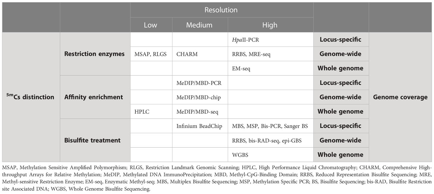
Table 1 Overview of methodologies for the analysis of DNA methylation (updated from (Anastasiadi, 2016).

1.1.1 Level 1. How are methylated loci identified?

5mCs must be identified and separated from the unmethylated ones (Cs). The processes of distinction between the two types of cytosines can be further divided into three general sub-levels, detailed below (Table 1 for an overview), that are not mutually exclusive and that in some cases are used in combination (Rauluseviciute et al., 2019):

1) Restriction enzymes. There are restriction enzymes which function differently when they encounter 5mCs and Cs. This property can be used to distinguish between the two types of Cs and ultimately identify their methylation status. Common isoschizomers, like MspI and HpaII, are used. For instance, these enzymes recognize the same sequence pattern (5’-CCGG-3’), however, MspI cuts at those sites where the internal C is methylated in the two complementary DNA strands, while HpaII is functional in those with methylation of the external C in one or both of the complementary DNA strands. The Methylation Sensitive Amplified Polymorphism (MSAP) (Reyna-Lopez et al., 1997; Xu et al., 2000) and the Restriction Landmark Genomic Scanning (RLGS (Hatada et al., 1991); are examples of approaches using methylation-sensitive restriction enzyme (Table 1).

2) Antibodies. This approach is based on the use of antibodies that show specificity against 5mC or of recombinant proteins which have been developed to contain a methyl-CpG binding domain (MBD; e.g (Aberg et al., 2012). These processes end up enriching the fraction of chromatin that is methylated. Methylated DNA ImmunoPrecipitation (MeDIP) (Jacinto et al., 2008) and Methyl-CpG-Binding Domain (MBD) (Jacinto et al., 2008; Nair et al., 2011) are examples of affinity-based approaches (Table 1) with MeDIP using a monoclonal antibody specific for 5mCs and MBD-based strategies using methyl-CpG binding domain-based proteins (MBDCap) (Nair et al., 2011).

3) Bisulfite. The treatment of DNA with bisulfite involves a chemical reaction that converts unmethylated Cs into uracils in 3 steps. Methylated 5mCs also react with bisulfite but this reaction is extremely slow and 5mCs are favoured by the equilibrium. Thus, 5mCs essentially escape conversion and remain intact (Clark et al., 1994). This reaction functions, therefore, as a recorder of the original methylation status and downstream steps allow to register and recall it. Several techniques, ranging from locus-specific to whole-genome, take advantage of the bisulfite properties in order to analyze the DNA methylation levels, like the Methylation-specific PCR (MSP) or the Whole Genome Bisulfite Sequencing (WGBS; Table 1). Bisulfite conversion of DNA is considered the “gold standard” in DNA methylation analysis because it allows the identification of the methylation status of each interrogated cytosine. However, limitations exist for bisulfite conversion methods as well. Methylation of a cytosine is a binary state (methylated or not methylated) in a given cell at a given time. Bisulfite sequencing reflects the relative proportion of Us/Cs at a given position, when sequencing tissues due to cell heterogeneity, and not the binary state of a specific cytosine unless single cell sequencing is performed. Methods based on bisulfite treatment of DNA are used for epigenetic clock construction.

1.1.2 Level 2. What is the resolution used?

The methylation profiling methods can have variable resolution, where higher resolution means information retrieval at the level of nucleotide and lower resolution means information retrieval at a larger genomic scale. In Table 1, an overview of the different methodologies for the analysis of DNA methylation with their corresponding resolution is provided. The resolution can broadly be grouped into the following three categories:

1) Low resolution. These techniques typically allow to obtain information on the global 5mC content. This is useful in order to conclude whether there are overall differences in the global methylation content or not, e.g., between control and treatment or disease group. Nevertheless, where exactly in the genome these differences occur remains unknown.

2) Medium resolution. Here, apart from global differences, an approximate location of the 5mCs is obtained. This is the case, for instance, of MeDIP-seq, where the methylated fraction of the immunoprecipitated DNA is sequenced and the differences can be located within a region that corresponds to the length of the sequenced fragment.

3) Single nucleotide resolution. In this case, the precise location of both 5mCs and Cs is obtained. This means that the exact position of 5mCs and Cs can be mapped to genomic coordinates that include 3 numbers: chromosome, start position, end position. For example, one obtains the information that in chromosome 1, start position=253, end position=254, there is a 5mC. Single nucleotide resolution is needed to construct an epigenetic clock.

1.1.3 Level 3. Which part of the genome is targeted?

The part of the genome that is investigated following the separation of Cs is also variable. In Table 1 an overview of the different methodologies for the analysis of DNA methylation with their relative CpG/genome coverage is provided. They can be broadly grouped into three categories according to this criterion as well:

1) Locus-specific. The amount of 5mCs and Cs is measured within target regions of interest typically spanning 10^-1–10² CpGs. The target region of interest can be a specific gene, regulatory region of a gene, genomic regions within a gene such as exons, introns or 5’UTRs, or any other genomic region that is a priori interesting and therefore can be a target for the analysis of its DNA methylation.

2) Genome-wide. The amount of 5mCs and Cs is measured within a part of the genome that is considered representative of the overall genome. The part of the genome is in the order of 10⁵–10⁶ CpGs and is representative because usually it is enriched for sites that can be methylated. For example, after digestion with enzymes that specifically recognize sites that include CpGs.

3) Whole-genome. The amount of 5mCs and Cs is measured across the whole genome covering more than 10⁶ CpGs. The entire genome is interrogated for its methylation levels, there is no reduction for specific regions or representative parts, but rather information on every single basis is obtained.

2 DNA methylation analysis using bisulfite sequencing

In the last years, high throughput sequencing (HTS) approaches have been used extensively to analyze the DNA methylation patterns in many different situations. The technique that combines the best possible way to distinguish 5mCs, single nucleotide resolution and whole genome coverage is Whole Genome Bisulfite Sequencing (WGBS), which is a HTS-based approach that uses bisulfite conversion to allow the distinction between 5mCs and Cs and interrogates the whole genome at single nucleotide resolution (Bock, 2012). Other HTS-based approaches that use bisulfite conversion, but analyze only a part of the genome are: Reduced Representation Bisulfite Sequencing (RRBS) (Gu et al., 2011; Klughammer et al., 2015), Bisulfite-converted Restriction site Associated DNA sequencing (bis-RAD-seq) (Trucchi et al., 2016), epiRADseq (Schield et al., 2016) and epi-GBS (van Gurp et al., 2016; Gawehns et al., 2022). Furthermore, targeted approaches such as BisPCR² (Bernstein et al., 2015), Multiplex Bisulfite Sequencing (MBS) (Anastasiadi et al., 2018) or others (Masser et al., 2013; Korbie et al., 2015; Roeh et al., 2018) are also HTS-based techniques that make use of bisulfite conversion but for a targeted part of the genome. Oxford Nanopore Technology sequencing is expected to vary for the basic bioinformatics steps, however, the statistical analysis including machine learning model building will be essentially the same (section 3). The HTS methods used for epigenetic clocks in fish species until now include RRBS, bis-RAD-seq, MBS and BisPCR² (see Table 1, Piferrer and Anastasiadi, 2023).

Different epigenetic clocks can be developed using different CpGs across the genome in different combinations, depending on the original dataset and the machine learning model. Around 20% of the Illumina 450K CpGs (90000 CpGs) can be used for epigenetic clocks (Porter et al., 2021). Taking this information into account, WGBS (>10⁶ CpGs) or RRBS (10³-10⁶ CpGs) may produce a large amount of unnecessary data and workload, while bis-RAD-seq or epiRADseq (10³-10⁵ CpGs) are expected to produce a good balance of informative CpGs without excess. Targeted approaches (e.g., MBS 10^-1-10² CpGs) will be more relevant when prior information is available.

2.1 Bioinformatics workflow for bisulfite sequencing

All HTS-derived data produced from methods that use bisulfite conversion share some common characteristics. A summary workflow allows to distinguish the steps of quality controls, filtering/trimming, alignment/mapping, methylation extraction and analysis (Figure 1).

FIGURE 1

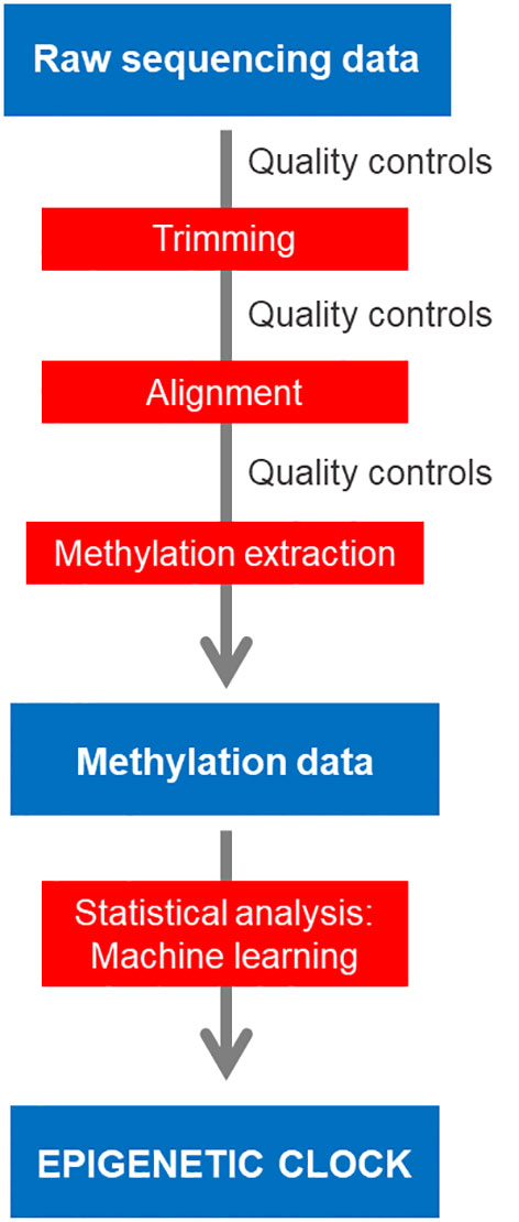
Figure 1 Workflow for bioinformatics analysis of bisulfite sequencing data for epigenetic clock construction.

Processing of HTS-derived data always initiates with the appropriate quality controls of the raw sequencing data obtained followed by filtering of the data that fall below the specified thresholds. Adapters or indices have usually been added to the DNA fragments during the preparation of the libraries and are used to demultiplex the samples if needed. Their sequences also usually need to be removed from the data (trimming) otherwise they might influence the downstream steps of the workflow. Once adapters have been trimmed and low quality reads filtered out, the reads are aligned against the genome which, importantly, must have been previously bisulfite converted in silico. This is because bisulfite treatment converts the unmethylated cytosines of the genome into uracils, which are in turn converted into thymines (Ts) after amplification by PCR. This process results in many genomic sites in the sequenced reads that fail to map to the genome because the original sites have been lost and thus, they cannot match. Moreover, after PCR amplification, the complementary DNA strand contains adenines (As) instead of guanines (Gs) in the positions where the C was unmethylated and has been converted into T. Thus, the procedure through which the sequenced reads are aligned to the genome needs to take into account these mismatches and considerations. Different tools have been developed to convert and map bisulfite sequencing data (See section 2.4.). A reference genome is not a pre-requisite for applying bisulfite sequencing since alternative bioinformatics procedures have been developed to assist the analysis, e.g., ad hoc genomes can be deduced from RRBS reads (Klughammer et al., 2015) or for bs-RAD-seq, a standard RAD-seq reduced representation genome can be used (Trucchi et al., 2016).

Once reads have been successfully mapped, the information of the methylation status has to be extracted at each C position of the genome, a process called methylation extraction or methylation calling. Usually, the final methylation of a given C is calculated according to the proportion of 5mCs and Cs found in that position: their sum equals to the coverage of a position and is the denominator in the equation where the numerator is the number of 5mCs. This value may be expressed as (5mCs/5mCs+Cs) and thus the methylation values will range from 0 to 1, or can be expressed as percentage, (5mCs/5mCs+Cs) multiplied by 100, and thus the methylation values will range from 0 to 100 (more details in section 2.5).

2.2 Quality controls

Modern sequencing platforms (e.g., Illumina) usually include the corresponding software which automatically performs the demultiplexing steps required prior to sample analysis and thus the corresponding set of files for each sample are obtained. In the case of single-end sequencing one file per sample is produced, while in the case of paired-end sequencing two files are produced per sample, each one of them refers to the forward and reverse read.

The standard format for these files is the FASTQ. FASTQ is a text-based format to store the sequences which includes more information than the older FASTA format which included only the sequence. In FASTQ, each read is unique and contains a sequence identifier and there is further information on the specific quality of the read. The quality of the reads is mainly measured by the Phred score which is a property logarithmically related to the base-calling error probabilities. A Phred score of 10, means that there is a 1 in 10 probability of incorrect base call and a 90% accuracy in base calls. A Phred score of 30 means that there is a 1 in 100 probability of incorrect base call and a 99.9% accuracy in base calls. Typically, Phred scores below 20, which equals to 99% accuracy of base call, are excluded from downstream analysis.

Quality controls are usually performed by a range of open source software packages, the most common of which is FASTQC (Andrews, 2010). In case several samples are to be evaluated at once, the MultiQC (Ewels et al., 2016) can be useful for simultaneous assessment of quality (see indicators below). These tools allow to assess the data quality via a variety of plots and statistics (Figures 2A–D), namely:

1) Sequence counts. The number of sequences counted for each sample.

2) Sequence quality histograms. The mean Phred score across each base position in the read.

3) Per sequence quality scores. The total number of reads plotted against the average Phred quality scores over the full read.

4) Per base sequence content. The percent of bases called for each of the four nucleotides (e.g., 30% A, 40% T, 20% C, 10% G) at each position (e.g, position 1-150 for a 150 bp read sequencing) across all reads.

5) Per sequence GC content. The number of reads plotted against the GC% per read.

6) Per base N content. The percent of bases at each position of the read for which no base could be called and are therefore coded as “N”.

7) Sequence length distribution. The distribution of lengths across all reads.

8) Sequence duplication levels. The percent of reads of a specific sequence that are present repeatedly inside the file and can be an indicator of PCR duplication.

9) Overrepresented sequences. Sequences that appear more times than expected.

10) Adapter content. Cumulative plot of the fraction of reads where the adapters used for library construction are identified.

FIGURE 2

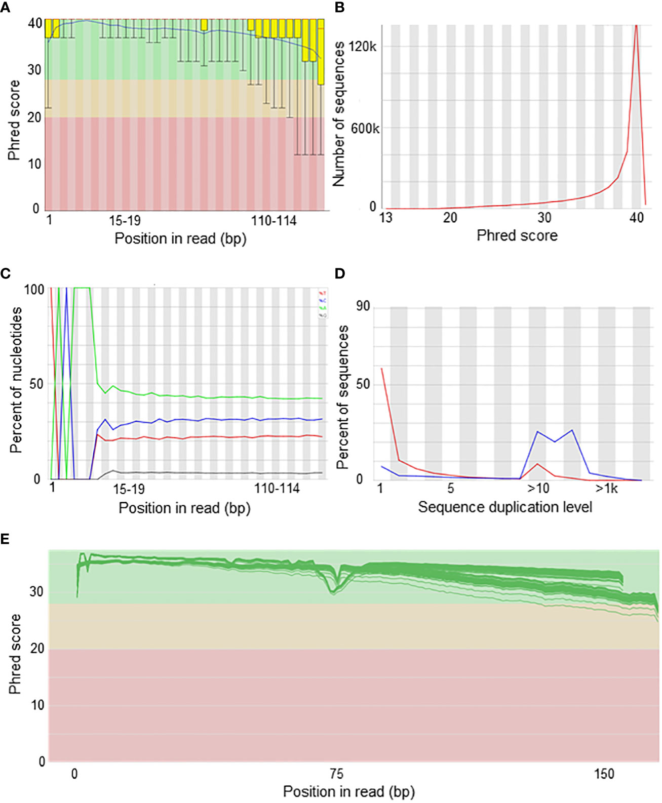
Figure 2 Quality control of sequencing data. Examples of plots from bis-RAD-seq experiment (own data). (A) Per base sequence quality shows the distribution of Phred quality of the bases (y-axis) along the length of the reads from base 0 to 150 (x-axis). (B) Per sequence quality scores shows the mean sequence quality as assessed by the Phred score (x-axis) in the number of overall sequences (y-axis). (C) Per base sequence content show the percentage of the four bases (T in red, C in blue, A in green and G in brown) along the length of the read from position 0 to 150 (x-axis). (D) The sequence duplication levels show the percent of sequences and their corresponding duplication levels (x-axis). (E) Simultaneous visualization of per base sequence quality from multiple samples by MultiQC software. The distribution of Phred quality of the bases (y-axis) along the length of the reads from base 0 to 150 (x-axis) is shown and green lines represent multiple samples.

Sequence quality scores below 30 are nowadays considered unacceptable. However, interpretation of the rest of the metrics will be specific to the technique and sequencing platform used, since high duplication levels are inherent to enrichment (e.g., RRBS) or targeted techniques, but may indicate a problem with WGBS data.

On the other hand, the simultaneous visualization of multiple quality controls (QC) can be obtained by the MultiQC software (Figure 2E). A drop of quality below the available threshold at the end of the read is expected in general and for long reads (300 bp) in particular.

Example code of running FASTQC in all available fq files:

fastqc –nogroup -q -t 2 -o output_fastq_raw *.fq.gz

Example code of running MultiQC in the output of FASTQC:

multiqc output_fastqc_raw -i Fastqc-Raw

2.3 Trimming

Several open source packages are available for trimming (Table 2). Trimming of low quality reads can significantly improve the quality of the data to process and all downstream workflow, as a minimum in terms of Phred scores Low quality Phred scores (<20) would be associated with too high probabilities of erroneously called bases, one nucleotide, e.g,. A, instead of another, e.g., C. Thus, they cannot be accepted in a HTS experiment. Quality controls are performed again after the trimming procedure as well and are useful to visualize the improvements.

TABLE 2

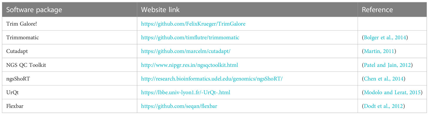
Table 2 Trimming software.

Example code of running Trimmomatic on WGBS data:

java -jar -Xms8G -Xmx8G

/software/Trimmomatic-0.36/trimmomatic.jar PE -threads 3

/raw_data/sample1_1.fq.gz

/raw_data/sample1_2.fq.gz

/trimmed_data/sample1_trimmed_R1.fastq

/trimmed_data/sample1_trimmed_R2.fastq

ILLUMINACLIP:/trimmed_data/adapters.fasta:2:30:10

SLIDINGWINDOW:5:20 MINLEN:50 HEADCROP:10 LEADING:5 TRAILING:5

2.4 Alignment

Bisulfite conversion depletes the genome of unmethylated cytosines which represents a challenge for the normal alignment procedure of reads to a large reference genome. Softwares developed for standard alignment procedures are not adequate in this case due to the conversion effect (Laird, 2010). This challenge has been circumvented by two different algorithms:

1) Wild card aligners. In this case, the Cs of the genome are replaced by Y which is the wild-card letter that is able to match both Cs and Ts, equivalent to Cs and 5mCs in the original molecule. Otherwise, these aligners modify the alignment score matrix in a manner that allows mismatch between Cs in the original molecule and Ts in the sequence of the read. Examples of wild card aligners include BSMAP and RRBSMAP (Xi and Li, 2009; Xi et al., 2012).

2) Three-letter aligners. In this case, all the Cs are converted into Ts in both the reads to be aligned and in the genomic sequence. The alignment is simplified and carried out using only three-letters of the nucleotide alphabet with C excluded. In this case, any standard aligner can be used at the lower level of the package, such as Bowtie or Bowtie2 (Langmead et al., 2009). Examples of three-letter aligners include Bismark, bwa-meth and BS-Seeker (Chen et al., 2010; Krueger and Andrews, 2011; Krueger et al., 2012, Pedersen et al., 2014).

Example code using bwa-meth:

Index reference genome

python/software/bwa-meth/bwameth.py index/genome/

species-genome.fasta

Align reads to reference genome

python

/software/bwa-meth/bwameth.py–threads 16

–reference/genome/species-genome.fasta

/trimmed_data/sample1_trimmed_R1.fastq

/trimmed_data/sample1_trimmed_R2.fastq

| samtools view -Sb -q 10 - >/alignments/sample1.bam

Example code using Bismark:

bismark

/reference/genome/

-1 sample1_trimmed_R1.fastq

-2 sample1_trimmed_R2.fastq

–non_directional –un -o alignments

bismark

/software/bismark/Genome/

-1 sample1_trimmed_R1. fastq

-2 sample1_trimmed_R2.fastq

–non_directional –un -o alignments

Wild card aligners typically result in higher genomic coverage, but also in the introduction of bias towards higher DNA methylation as compared to three-letter aligners. This is relevant mainly in parts of the genome such as repetitive sequences. When selecting an aligner, considerations such as speed, computer memory and program use are more important (Bock, 2012). A recent comprehensive comparison of the most commonly used aligners should be consulted before executing this step (Nunn et al., 2021). In any case, mapping of the reads to the genome needs to be precise because otherwise it would result in biased DNA methylation levels calculated on the basis of methylated and unmethylated reads (Bock et al., 2010).

2.5 Methylation extraction

The methylation state of each C is extracted according to the alignments. Cytosines from the aligned sequences are transcribed into a table format where each row corresponds to a cytosine and its genomic position according the chromosome and position, methylation state and strand. Coding of this information within the table depends on the software used. For example, the Bismark (Krueger and Andrews, 2011) primary alignment output codes cytosines depending on the context, as z in CpG context, x in CHG context and h in CHH context. Methylation status is coded as uppercase (Z, X, H) for methylated and lowercase (z, x, h) for unmethylated. This information is transcribed into + for methylated and - for unmethylated cytosines in the methylation extraction file.

Example code using MethylDackel for use with methylKit:

MethylDackel extract –OT 0,0,0,145 –OB 3,0,6,0 –methylKit

-o/methylation_extraction/sample1.methylKit

/genome/species-genome.fasta

sample1-aligned.bam

Example code using Bismark:

bismark_methylation_extractor sample1_aligned.bam -p –

merge_non_CpG -o extraction –bedGraph –cutoff 1

2.6 Bisulfite conversion rate

Evaluation of bisulfite conversion efficiency is an important step of the whole procedure because if this fails, then conclusions on the methylation status of the cytosines are erroneous. Spike-in sequences of known methylation status may have been introduced during library preparation to assist with bisulfite conversion rate estimation. If not, bisulfite conversion rate can be estimated in silico. Tools like the ‘bsrate’ script of the MethPipe pipeline (Song et al., 2013) allow for an automatic calculation of the bisulfite conversion ratio. Otherwise, one can make use of the percent of Cs methylated in a CHH context where C is cytosine and H can be any nucleotide except of Gs. In this case, the percent of these Cs is subtracted from 100 and the result is the bisulfite conversion rate. In current DNA methylation analysis procedures, bisulfite conversion rates should be as high as possible. Typical good values are >99%.

3 Statistical analysis

3.1 Objective

The objective of this step is to identify CpGs the methylation levels of which allow to predict the age of an individual. The methylation of these CpGs may be decreasing or increasing with age with different slopes. The methylation of each CpG will be given a specific weight (coefficient) and their combination will be sufficient to predict age. These coefficients were shown to differ in the same CpGs between broad age groups in mammals, including humans (younger, middle-aged and older). Therefore, the extreme age groups should be considered with caution (Field et al., 2018) but nevertheless included for the development of the clock. The statistical analysis includes a typical machine learning model building (Figure 3). Building of machine learning models for age prediction follows the same principles as for any biological feature predicted from epigenetic biomarkers (Anastasiadi and Beemelmanns, 2023). The outcome variable is quantitative (age) and thus we deal with a regression problem aiming to predict the outcome variable on the basis of the independent variable(s) by means of a fitting curve explaining the input. When running a regression trying to predict a quantitative value (i.e. age) with many predictors (CpGs) results tend to overfit, reducing the predictive value. Penalized regression circumvent this problem by shrinking values of the predictors, being the recommended for age prediction based on CpG methylation (See Section 3.3).

FIGURE 3

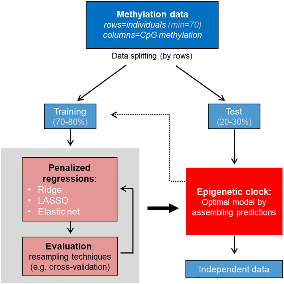
Figure 3 Workflow for machine learning model building for epigenetic clock. Data are split into training and test, model is tuned and evaluated using the training dataset, the optimal model is selected and evaluated using the test dataset. If model performance is not optimal, the procedure may be repeated using the training dataset. The age in independent data can be predicted by the optimal final model or “epigenetic clock”.

3.2 Data structure

The dataset consists of:

1) Biological samples that cover a defined age range. The total number of samples should ensure covering the full age range of the species considered, and may vary between species in the extremes of lifespan. In the published literature of fish epigenetic clocks, the total number of samples range between 10 in Northern red snapper and red grouper (Weber et al., 2021) and 141 in Australian lungfish (Mayne et al., 2021b) with mean 46 samples (Piferrer and Anastasiadi, 2023). These numbers maybe suboptimal, since the minimum sample size according to simulations using human and zebrafish (Danio rerio) data is 70 (Mayne et al., 2021a). If feasible, 134 samples should be ideally included according to the same simulations, a recommendation for all new piscine epigenetic clocks (Mayne et al., 2021a). In order to build a prediction model, these will have to be divided into training and test sets. The training set is used for the machine to learn, to fit the parameters of the model. The test set is an independent set of data which the model built predicts and thus serves as an evaluation dataset of the model fit. Usually, the original dataset is split in 70-80% of the observations into training and 20-30% of the observations into the test set, using random procedures.

2) The methylation levels of target CpGs. Depending on the technique used, the number of CpGs will be in the order of hundreds (e.g. MBS), thousands (e.g. bis-RAD-seq), hundreds of thousands (e.g. RRBS) or millions (e.g. WGBS). Since many epigenetic clocks across a genome are possible (Porter et al., 2021) and extremely accurate epigenetic clocks with only 3 carefully selected CpGs have been constructed in mice (Han et al., 2018), the number of CpGs analyzed are not expected to affect the overall accuracy. However, each epigenetic clock or model will be unique as will be the coefficients attributed to each CpG of the clock. This type of data is not independent, since the methylation of one CpG may depend on the methylation of its neighboring CpG and are characterized by strong multicollinearity, where a large number of CpGs may be closely related to each other. Genome-wide patterns of DNA methylation in vertebrates are bimodal with a specific CpGs showing 0 or 100% methylation.

3.3 Penalized regressions

In the development of epigenetic clocks we are dealing with a large multivariate dataset, where the number of variables (the different CpGs, at least the ones initially analyzed) is much, much higher than the number of samples (biological samples). Thus, the standard linear model is not suitable to use. A way to circumvent the structure of the dataset is to use penalized regressions. This approach was already implemented by Horvath (2013) when constructing the first epigenetic clock in humans. Penalized regressions allow to construct linear regression models that are penalized when they have too many variables (Kassambara, 2018). The penalization occurs via the addition of a constraint in the equation (Bruce and Bruce, 2017). This increases bias but, importantly, reduces variance. The methodology to achieve this is shrinkage or regularization, which results in the shrinkage of some coefficients values to zero. This allows for exclusion of the variables (i.e., individual CpGs) that contribute less by shrinking their coefficient or in other words, to retain the minimum number of CpGs that are valuable for age prediction.

There are three most commonly used methods of penalized regression and typically they are all tested when constructing an epigenetic age prediction clock for a new species:

1) Ridge regression. The least contributing variables will have their coefficient very close to zero.

2) LASSO regression (Least Absolute Shrinkage and Selection Operator). The variables with the least contribution will be forced to be zero. This will produce models with reduced complexity as compared to ridge regression, where all variables are kept.

3) Elastic net regression. This type of penalized regression stands in between the previous two types, where some coefficients will be shrank, as in ridge regression, and some coefficients will be set to zero, as in LASSO.

There are advantages and disadvantages of each penalized regression type over the other that depend on the specific dataset. LASSO will perform better when there are few predictors with large coefficients and a lot of predictors with small coefficients, while ridge will perform better where there are a lot of predictors with similar coefficients. Ridge regression keeps all variables, therefore, is not recommended when genome-wide techniques have been used. In any case, parameters of the model have to be tuned and the model has to be selected by evaluating its performance, as explained below.

3.4 Machine learning model building

Penalized regressions are machine learning models and thus, to build them, a standard machine learning model building procedure should be followed (Figure 3). In aquatic organisms, machine learning methods for developing epigenetic biomarkers have been applied in limited cases, while the procedure has been recently reviewed in details (Anastasiadi and Beemelmanns, 2023).

Below we explain the typical workflow of the procedure that can be implemented in R using the specialized caret (Classification And REgression Training) package (Kuhn, 2008). Nevertheless, other packages or programming language (e.g., Python) can also be used to navigate the same workflow.

1) Data splitting. Data are split into at least 2 datasets that allow to later evaluate model performance. The training dataset contains 70-80% of the samples and is used to for algorithm training and parameter tuning. The test datasets contains the remaining 20-30% of samples and is used once the right model has been trained and selected to test whether the model can be generalized in unseen data. Ideally, training dataset is sufficiently large to be split further into training and validation dataset during model performance assessment. However, this is rarely the case and instead resampling techniques are used. With resampling, iterative splitting into training and validation datasets occurs and prediction errors of all splitting cycles are averaged at the end. K-fold cross-validation (CV) has been extensively used in fish epigenetic clock building. Data splitting can be performed using specific functions that randomly splits the dataset, while keeping track of the randomness by setting the seed to a specific number in R.

R code example:

library(tidymodels)

library(readr)

set.seed(123)

splits <- initial_split(meth.age.df, strata = age)

age_other <- training(splits)

age_test <- testing(splits)

Training set proportions by age class

age_other %>%

count(age) %>%

mutate(prop = n/sum(n))

Test set proportions by age class

age_test %>%

count(age) %>%

mutate(prop = n/sum(n))

2) Data preparation and pre-processing. This step may include a) exclusion of CpGs the methylation of which has zero or near-zero variance across ages in the training dataset; b) dealing with multicollinearity by identifying CpGs with correlated methylation –a common feature in this type of data–; c) data transformation of centering and scaling variables to mean 0 and standard deviation 1; d) imputation of missing values if necessary. Imputations can be performed by the mice (Multivariate Imputation by Chained Equations) package in R (van Buuren and Groothuis-Oudshoorn, 2011).

Correlation of CpG methylation with other biological parameters that we want to account for, such as diet, sex or other environmental factors, can be dealt with by exclusion of the correlated CpGs when lots of CpGs. This type of correlation is likely to be confounding factor in the model if these biological parameters are parallel to age (i.e., we have many samples of younger males and older females).

R code example:

a) Excluding features with zero or near-zero variance among groups

library(caret)

library(dplyr)

## Detect features and visualize them

nzv.cpg <- nearZeroVar(age_other, saveMetrics= TRUE, names=TRUE, freqCut = 85/15, uniqueCut = 50)

boxplot(nzv.cpg$percentUnique)

boxplot(nzv.cpg$freqRatio)

## Detect features, exclude them and save the object

nzv.cpg.list <- nearZeroVar(age_other, freqCut = 85/15, uniqueCut = 50) filteredDescr <- age_other[, -nzv.cpg.list] dim(filteredDescr)

b) Exclude highly correlated variables

highlyCorDescr <- findCorrelation(filteredDescr, cutoff = 0.8)

filteredDescr.cor <- filteredDescr[,-highlyCorDescr]

c) Transformation via preProcess data

preProcValues <- preProcess(filteredDescr.cor, method = c(“center”, “scale”))

trainTransformed <- predict(preProcValues, filteredDescr.cor)

d) Imputation of missing values

Method 1 using package “mice” (Multiple Imputation by Chained Equation)

library(mice)

init = mice(meth.age.df, maxit=0)

meth = init$method

predM = init$predictorMatrix

colnames(meth.age.df)

predM[, c("age")]=0

meth[c("age")]=""

set.seed(100)

imputed = mice(meth.age.df, method=meth, predictorMatrix=predM, m=5)

Method 2 using package “zoo” (Missing values replaced by the mean or other function of its group)

library(zoo)

meth.age.df.na <- na.aggregate(meth.age.df)

3) Model tuning. The best tuning parameters for alpha and lambda of the penalized regression algorithm are selected. Alpha defines the type of regression with α=0 ridge, α=1 LASSO and 0<α<1 elastic net, while lambda defines the amount of shrinkage. Lambda will be automatically selected to minimize prediction error. Simultaneously feature selection, i.e., selection of the most informative CpGs, is performed.

4) Model evaluation is performed using resampling techniques, k-fold CV, repeated CV or leave-one-out CV (LOOCV). The error will be minimized after several repeated rounds of dataset splitting and finally, the optimal model is selected.

R code example using caret (steps 3-4):

Define resampling technique to be used. Here we choose repeated cross-validation

fitControl <- trainControl(method = ‘repeatedcv’, number=10, repeats=10)

Define range of lambda to be tested

lambda <- 10^seq(-3, 3, length = 100)

Run penalized regressions. Examples of ridge, LASSO and elastic net regressions are shown here.

Ridge regression. This regression may not be relevant in cases of RRBS or WGBS data since it keeps all CpGs available, but may be worth in cases of targeted methods (e.g., MBS).

set.seed(123)

ridge_model <- train(age ~., data = trainTransformed, method = “glmnet”, trControl = fitControl, tuneGrid = data.frame(alpha = 0, lambda = 10^seq(-3, 3, length = 100)), tuneLength = 10)

LASSO

set.seed(123)

lasso_model <- train(age ~., data = trainTransformed, method = “glmnet”, trControl = fitControl, tuneGrid = data.frame(alpha = 1, lambda = 10^seq(-3, 3, length = 100)), tuneLength = 10)

In Elastic net best tuning of both lambda and alpha will be automatically selected

set.seed(123)

elastic_model <- train(age ~., data = trainTransformed, method = “glmnet”, trControl = fitControl, tuneLength = 10)

Elastic net with alpha set to 0.5 and best tuning of lambda will be automatically selected

set.seed(123)

elastic_model.05 <- train(age ~., data = trainTransformed, method = “glmnet”, trControl = fitControl, tuneGrid = data.frame(alpha = 0.5, lambda = 10^seq(-3, 3, length = 100)), tuneLength = 10)

Compare metrics of the models

models_compare <- resamples(list(R=ridge_model, LM=lasso_model, EM=elastic_model, EM05=elastic_model.05))

summary(models_compare)

Count features (CpGs) kept by each model. An ideal piscine epigenetic clock with wide application would contain as few CpGs as possible without compromising accuracy and precision. Example using elastic net.

sum(coef(elastic_model$finalModel, elastic_model$bestTune$lambda)!=0)

Compare metrics in the training datasets

Ridge

predicted.age <- predict.train(ridge_model)

postResample(pred = predicted.age, trainTransformed$age)

cor.test(predicted.age, trainTransformed$age)

LASSO

predicted.age <- predict.train(lasso_model)

postResample(pred = predicted.age, trainTransformed$age)

cor.test(predicted.age, trainTransformed$age)

Elastic net

predicted.age <- predict.train(elastic_model)

postResample(pred = predicted.age, trainTransformed$age)

cor.test(predicted.age, trainTransformed$age)

5) Assembling predictions. The optimal model needs to be further evaluated using the test dataset in order to assess how well it can generalize. The final model will be then built using the optimal model run on the whole training dataset.

R code example: Compare metrics in the test dataset

Ridge

predict.ridge.test <- predict(ridge_model, testTransformed)

postResample(pred = predict.ridge.test, testTransformed$age)

cor.test(predict.ridge.test, testTransformed$age)

LASSO

predict.lasso.test <- predict(lasso_model, testTransformed)

postResample(pred = predict.lasso.test, testTransformed$age)

cor.test(predict.lasso.test testTransformed$age

Elastic net

predict.enet.test <- predict(elastic_model, testTransformed)

postResample(pred = predict.enet.test, testTransformed$age)

cor.test(predict.enet.test, testTransformed$age)

Build and evaluate the final model

finalmodelCtrl <- trainControl(method = “none”)

set.seed(123)

final <- train(age ~., data = trainTransformed, method = "glmnet", trControl=finalmodelCtrl, tuneGrid = expand.grid(alpha = bestalpha, lambda = bestlambda))

predicted.final.train <- predict(final, trainTransformed)

cor.test(predicted.final.train, trainTransformed$age)

Evaluation of models during training as well as at the final model is done by assessing the predictive accuracy via loss functions comparing predicted age vs actual age. The measures to take into account and report include:

a) Root Mean Squared Error (RMSE) = average deviation of the predictions from the observations.

b) Mean Absolute Error (MAE) = average of the absolute differences between the observed and predicted values.

c) R² = the squared correlation between the observed and predicted values. This value shows how well the selected variables (methylation of CpGs) explain the variability of the dependent variable (age).

The errors should be minimized while the R² should be maximized.

Epigenetic clocks are considered valid if the correlation (R) is higher than 0.80 in large independent data covering a broad age range (Horvath and Raj, 2018). Piscine epigenetic clocks show a mean correlation of 0.93 (Piferrer and Anastasiadi, 2023), while higher values are also possible. Precision reported as MAE is used with actual time units (days, months or years) and shows a mean of 0.87 years in piscine clocks, or an average of about 3.5% of the total lifespan (Piferrer and Anastasiadi, 2023).

4 Conclusions 

Epigenetic clocks for age prediction are typically constructed using DNA methylation sequencing technologies that involve the use of bisulfite conversion and provide information at single nucleotide resolution. Bioinformatic analysis of the data follows mostly standard procedures of sequencing reads analysis, however, care should be taken to account for C to T conversion during the alignment step. Methylation values are extracted per base and this results in the dataset consisting of individual fish aged samples as rows and methylation values of interrogated CpGs as columns. This multivariate dataset is submitted to machine learning procedures aiming to select features, i.e., CpGs the methylation of which is enough to predict age. The machine learning procedures used are penalized (or regularized) regressions which fit well the structure of the multivariate dataset. At the end of the procedure, the optimal model or “epigenetic clock” is constructed. This constitutes a molecular resource to be implemented by scientists and managers for accurate age prediction of fish. The simultaneous interrogation of the methylation of a few target CpGs forming the epigenetic clock of a large amount of samples in a ready-to-use kit constitutes the ultimate goal for application of this HTS to fisheries and conservation.

Author contributions

DA: Conceived and wrote the manuscript. FP: Conceived and edited the manuscript. All authors contributed to the article and approved the submitted version.

Funding

Funded through EU Contract – EASME/EMFF/2017/1.3.2.10/SI2.790889 to FP.

Acknowledgments

We would like to thank Drs. Gary Carvalho, Sissel Jentoft, Laszlo Orban, Allan Tucker and two reviewers for constructive criticisms and suggestions for improvement to an earlier version of this manuscript.

Conflict of interest

DA is employed by The New Zealand Institute for Plant and Food Research Limited.

The remaining authors declare that the research was conducted in the absence of any commercial or financial relationships that could be construed as a potential conflict of interest.

Publisher’s note

All claims expressed in this article are solely those of the authors and do not necessarily represent those of their affiliated organizations, or those of the publisher, the editors and the reviewers. Any product that may be evaluated in this article, or claim that may be made by its manufacturer, is not guaranteed or endorsed by the publisher.

Author disclaimer

The information and views set out in this publication are based on scientific data and information collected under Service Contract “Improving cost-efficiency of fisheries research surveys and fish stocks assessments using next-generation genetic sequencing methods [EMFF/2018/015]” signed with the European Climate, Infrastructure and Environment Executive Agency (CINEA) and funded by the European Union. The information and views set out in this publication are those of the author(s) and do not necessarily reflect the official opinion of CINEA or of the European Commission. Neither CINEA nor the European Commission can guarantee the accuracy of the scientific data/information collected under the above Specific Contract or the data/information included in this publication. Neither CINEA nor the European Commission or any person acting on their behalf may be held responsible for the use which may be made of the information contained therein.

References

Aberg K. A., McClay J. L., Nerella S., Xie L. Y., Clark S. L., Hudson A. D., et al. (2012). MBD-seq as a cost-effective approach for methylome-wide association studies: Demonstration in 1500 case–control samples. Epigenomics 4, 605–621. doi: 10.2217/epi.12.59

PubMed Abstract | CrossRef Full Text | Google Scholar

Anastasiadi D. (2016). Intrinsic and environmental influences on DNA methylation and gene expression in fish. In: TDX (Tesis doctorals en xarxa). Available at: http://www.tdx.cat/handle/10803/511360 (Accessed April 8, 2020).

Google Scholar

Anastasiadi D., Beemelmanns A. (2023). Development of epigenetic biomarkeres in aquatic organisms in Epigenetics in aquaculture. Eds. Piferrer F., Wang H. (Hoboken, NJ: John Wiley & Sons Ltd).

Google Scholar

Anastasiadi D., Piferrer F. (2020). A clockwork fish: Age prediction using DNA methylation-based biomarkers in the European seabass. Mol. Ecol. Resour 20, 387–397. doi: 10.1111/1755-0998.13111

PubMed Abstract | CrossRef Full Text | Google Scholar

Anastasiadi D., Vandeputte M., Sánchez-Baizán N., Allal F., Piferrer F. (2018). Dynamic epimarks in sex-related genes predict gonad phenotype in the European sea bass, a fish with mixed genetic and environmental sex determination. Epigenetics 13, 988–1011. doi: 10.1080/15592294.2018.1529504

PubMed Abstract | CrossRef Full Text | Google Scholar

Andrews S. (2010). FastQC: A quality control tool for high throughput sequence data. Accessed January 29, 2023. https://www.bioinformatics.babraham.ac.uk/projects/fastqc/.

Google Scholar

Barros-Silva D., Marques C. J., Henrique R., Jerónimo C. (2018). Profiling DNA methylation based on next-generation sequencing approaches: New insights and clinical applications. Genes (Basel) 9, 429. doi: 10.3390/genes9090429

PubMed Abstract | CrossRef Full Text | Google Scholar

Bell C. G., Lowe R., Adams P. D., Baccarelli A. A., Beck S., Bell J. T., et al. (2019). DNA Methylation aging clocks: Challenges and recommendations. Genome Biol. 20, 249. doi: 10.1186/s13059-019-1824-y

PubMed Abstract | CrossRef Full Text | Google Scholar

Bernstein D. L., Kameswaran V., Le Lay J. E., Sheaffer K. L., Kaestner K. H. (2015). The BisPCR2 method for targeted bisulfite sequencing. Epigenet. Chromatin 8, 27. doi: 10.1186/s13072-015-0020-x

CrossRef Full Text | Google Scholar

Bertucci E. M., Mason M. W., Rhodes O. E., Parrott B. B. (2021). Exposure to ionizing radiation disrupts normal epigenetic aging in Japanese medaka. Aging 13, 22752–22771. doi: 10.18632/aging.203624

PubMed Abstract | CrossRef Full Text | Google Scholar

Biomarkers Definitions Working Group (2001). Biomarkers and surrogate endpoints: Preferred definitions and conceptual framework. Clin. Pharmacol. Ther. 69, 89–95. doi: 10.1067/mcp.2001.113989

PubMed Abstract | CrossRef Full Text | Google Scholar

Bock C. (2012). Analysing and interpreting DNA methylation data. Nat. Rev. Genet. 13, 705–719. doi: 10.1038/nrg3273

PubMed Abstract | CrossRef Full Text | Google Scholar

Bock C., Tomazou E. M., Brinkman A. B., Müller F., Simmer F., Gu H., et al. (2010). Quantitative comparison of genome-wide DNA methylation mapping technologies. Nat. Biotechnol. 28, 1106–1114. doi: 10.1038/nbt.1681

PubMed Abstract | CrossRef Full Text | Google Scholar

Bolger A. M., Lohse M., Usadel B. (2014). Trimmomatic: a flexible trimmer for illumina sequence data. Bioinformatics 30, 2114–2120. doi: 10.1093/bioinformatics/btu170

PubMed Abstract | CrossRef Full Text | Google Scholar

Bruce P., Bruce A. (2017). Practical statistics for data scientists: 50 essential concepts (Sebastopol, CA: O’Reilly Media, Inc).

Google Scholar

Carlberg C., Molnár F. (2014). The epigenome in Mechanisms of gene regulation (Springer, Netherlands).

Google Scholar

Chen P. Y., Cokus S. J., Pellegrini M. (2010). BS seeker: Precise mapping for bisulfite sequencing. BMC Bioinf. 11, 203. doi: 10.1186/1471-2105-11-203

CrossRef Full Text | Google Scholar

Chen C., Khaleel S. S., Huang H., Wu C. H. (2014). Software for pre-processing illumina next-generation sequencing short read sequences. Source Code Biol. Med. 9, 8. doi: 10.1186/1751-0473-9-8

PubMed Abstract | CrossRef Full Text | Google Scholar

Clark S. J., Harrison J., Paul C. L., Frommer M. (1994). High sensitivity mapping of methylated cytosines. Nucleic Acids Res. 22, 2990–2997. doi: 10.1093/nar/22.15.2990

PubMed Abstract | CrossRef Full Text | Google Scholar

Costa-Pinheiro P., Montezuma D., Henrique R., Jerónimo C. (2015). Diagnostic and prognostic epigenetic biomarkers in cancer. Epigenomics 7, 1003–1015. doi: 10.2217/epi.15.56

PubMed Abstract | CrossRef Full Text | Google Scholar

Deans C., Maggert K. A. (2015). What do you mean, “epigenetic”? Genetics 199, 887–896. doi: 10.1534/genetics.114.173492

PubMed Abstract | CrossRef Full Text | Google Scholar

Dodt M., Roehr J. T., Ahmed R., Dieterich C. (2012). FLEXBAR-flexible barcode and adapter processing for next-generation sequencing platforms. Biol. (Basel) 1, 895–905. doi: 10.3390/biology1030895

CrossRef Full Text | Google Scholar

Ewels P., Magnusson M., Lundin S., Käller M. (2016). MultiQC: summarize analysis results for multiple tools and samples in a single report. Bioinformatics 32, 3047–3048. doi: 10.1093/bioinformatics/btw354

PubMed Abstract | CrossRef Full Text | Google Scholar

Field A. E., Robertson N. A., Wang T., Havas A., Ideker T., Adams P. D. (2018). DNA Methylation clocks in aging: Categories, causes, and consequences. Mol. Cell 71, 882–895. doi: 10.1016/j.molcel.2018.08.008

PubMed Abstract | CrossRef Full Text | Google Scholar

Gawehns F., Postuma M., van Antro M., Nunn A., Sepers B., Fatma S., et al. (2022). epiGBS2: Improvements and evaluation of highly multiplexed, epiGBS-based reduced representation bisulfite sequencing. Mol. Ecol. Resour. 22, 2087–2104. doi: 10.1111/1755-0998.13597

PubMed Abstract | CrossRef Full Text | Google Scholar

Grosjean H. (2013) Nucleic acids are not boring long polymers of only four types of nucleotides: A guided tour (Landes Bioscience). Available at: http://www.ncbi.nlm.nih.gov/books/NBK6489/ (Accessed July 26, 2016).

Google Scholar

Guevara E. E., Lawler R. R. (2018). Epigenetic clocks. Evolutionary Anthropol: Issues News Rev. 27, 256–260. doi: 10.1002/evan.21745

CrossRef Full Text | Google Scholar

Gu H., Smith Z. D., Bock C., Boyle P., Gnirke A., Meissner A. (2011). Preparation of reduced representation bisulfite sequencing libraries for genome-scale DNA methylation profiling. Nat. Protoc. 6, 468–481. doi: 10.1038/nprot.2010.190

PubMed Abstract | CrossRef Full Text | Google Scholar

Han Y., Eipel M., Franzen J., Sakk V., Dethmers-Ausema B., Yndriago L., et al. (2018). Epigenetic age-predictor for mice based on three CpG sites. eLife 7, e37462. doi: 10.7554/eLife.37462

PubMed Abstract | CrossRef Full Text | Google Scholar

Hatada I., Hayashizaki Y., Hirotsune S., Komatsubara H., Mukai T. (1991). A genomic scanning method for higher organisms using restriction sites as landmarks. Proc. Natl. Acad. Sci. 88, 9523–9527. doi: 10.1073/pnas.88.21.9523

CrossRef Full Text | Google Scholar

Hayes B. J., Nguyen L. T., Forutan M., Engle B. N., Lamb H. J., Copley J. P., et al. (2021). An epigenetic aging clock for cattle using portable sequencing technology. Front. Genet. 12. doi: 10.3389/fgene.2021.760450

CrossRef Full Text | Google Scholar

Horvath S. (2013). DNA Methylation age of human tissues and cell types. Genome Biol. 14, R115. doi: 10.1186/gb-2013-14-10-r115

PubMed Abstract | CrossRef Full Text | Google Scholar

Horvath S., Raj K. (2018). DNA Methylation-based biomarkers and the epigenetic clock theory of ageing. Nat. Rev. Genet. 19, 371–384. doi: 10.1038/s41576-018-0004-3

PubMed Abstract | CrossRef Full Text | Google Scholar

Jacinto F. V., Ballestar E., Esteller M. (2008). Methyl-DNA immunoprecipitation (MeDIP): hunting down the DNA methylome. Biotechniques 44, 35. doi: 10.2144/000112708

PubMed Abstract | CrossRef Full Text | Google Scholar

Kassambara A. (2018). Machine learning essentials: Practical guide in r (France: STHDA).

Google Scholar

Klughammer J., Datlinger P., Printz D., Sheffield N. C., Farlik M., Hadler J., et al. (2015). Differential DNA methylation analysis without a reference genome. Cell Rep. 13, 2621–2633. doi: 10.1016/j.celrep.2015.11.024

PubMed Abstract | CrossRef Full Text | Google Scholar

Korbie D., Lin E., Wall D., Nair S. S., Stirzaker C., Clark S. J., et al. (2015). Multiplex bisulfite PCR resequencing of clinical FFPE DNA. Clin. Epigenet. 7, 28. doi: 10.1186/s13148-015-0067-3

CrossRef Full Text | Google Scholar

Krueger F., Andrews S. R. (2011). Bismark: A flexible aligner and methylation caller for bisulfite-seq applications. Bioinformatics 27, 1571–1572. doi: 10.1093/bioinformatics/btr167

PubMed Abstract | CrossRef Full Text | Google Scholar

Krueger F., Kreck B., Franke A., Andrews S. R. (2012). DNA Methylome analysis using short bisulfite sequencing data. Nat. Methods 9, 145–151. doi: 10.1038/nmeth.1828

PubMed Abstract | CrossRef Full Text | Google Scholar

Kuhn M (2008). Building predictive models in R using the caret package. J Stat Softw. 28, 1–26. doi: 10.1038/nrg2732

PubMed Abstract | CrossRef Full Text | Google Scholar

Laird P. W. (2010). Principles and challenges of genome-wide DNA methylation analysis. Nat. Rev. Genet. 11, 191. doi: 10.1038/nrg2732

PubMed Abstract | CrossRef Full Text | Google Scholar

Langmead B., Trapnell C., Pop M., Salzberg S. L. (2009). Ultrafast and memory-efficient alignment of short DNA sequences to the human genome. Genome Biol. 10, R25. doi: 10.1186/gb-2009-10-3-r25

PubMed Abstract | CrossRef Full Text | Google Scholar

Liu W., Cui Y., Ren W., Irudayaraj J. (2019). Epigenetic biomarker screening by FLIM-FRET for combination therapy in ER+ breast cancer. Clin. Epigenet. 11, 16. doi: 10.1186/s13148-019-0620-6

CrossRef Full Text | Google Scholar

Martin M. (2011). Cutadapt removes adapter sequences from high-throughput sequencing reads. EMBnet.journal 17, 10–12. doi: 10.14806/ej.17.1.200

CrossRef Full Text | Google Scholar

Masser D. R., Berg A. S., Freeman W. M. (2013). Focused, high accuracy 5-methylcytosine quantitation with base resolution by benchtop next-generation sequencing. Epigenet. chromatin 6, 33. doi: 10.1186/1756-8935-6-33

CrossRef Full Text | Google Scholar

Mayne B., Berry O., Jarman S. (2021a). Optimal sample size for calibrating DNA methylation age estimators. Mol. Ecol. Resour. 21, 2316–2323. doi: 10.1111/1755-0998.13437

PubMed Abstract | CrossRef Full Text | Google Scholar

Mayne B., Espinoza T., Roberts D., Butler G. L., Brooks S., Korbie D., et al. (2021b). Nonlethal age estimation of three threatened fish species using DNA methylation: Australian lungfish, Murray cod and Mary river cod. Mol. Ecol. Resour. 21, 2324–2332. doi: 10.1111/1755-0998.13440

PubMed Abstract | CrossRef Full Text | Google Scholar

Mayne B., Korbie D., Kenchington L., Ezzy B., Berry O., Jarman S. (2020). A DNA methylation age predictor for zebrafish. Aging 12, 24817–24835. doi: 10.18632/aging.202400

PubMed Abstract | CrossRef Full Text | Google Scholar

Modolo L., Lerat E. (2015). UrQt: An efficient software for the unsupervised quality trimming of NGS data. BMC Bioinf. 16, 1–8. doi: 10.1186/s12859-015-0546-8

CrossRef Full Text | Google Scholar

Nair S. S., Coolen M. W., Stirzaker C., Song J. Z., Statham A. L., Strbenac D., et al. (2011). Comparison of methyl-DNA immunoprecipitation (MeDIP) and methyl-CpG binding domain (MBD) protein capture for genome-wide DNA methylation analysis reveal CpG sequence coverage bias. Epigenetics 6, 34–44. doi: 10.4161/epi.6.1.13313

PubMed Abstract | CrossRef Full Text | Google Scholar

Nunn A., Otto C., Stadler P. F., Langenberger D. (2021). Comprehensive benchmarking of software for mapping whole genome bisulfite data: From read alignment to DNA methylation analysis. Brief Bioinform. 22, bbab021. doi: 10.1093/bib/bbab021

PubMed Abstract | CrossRef Full Text | Google Scholar

Ortega-Recalde O., Hore T. A. (2023). Analythical methods to study the epigenome in Epigenetics in aquaculture. Eds. Piferrer F., Wang H. (Hoboken, NJ: John Wiley & Sons Ltd).

Google Scholar

Patel R. K., Jain M. (2012). NGS QC toolkit: A toolkit for quality control of next generation sequencing data. PloS One 7, e30619. doi: 10.1371/journal.pone.0030619

PubMed Abstract | CrossRef Full Text | Google Scholar

Pedersen B. S., Eyring K., De S., Yang I. V., Schwartz D. A. (2014). Fast and accurate alignment of long bisulfite-seq reads. arXiv. doi: 10.48550/arXiv.1401.1129

CrossRef Full Text | Google Scholar

Pfeifer G. P. (2016). Epigenetics: An elusive DNA base in mammals. Nature 532, 319–320. doi: 10.1038/nature17315

PubMed Abstract | CrossRef Full Text | Google Scholar

Piferrer F, Anastasiadi D (2023). Age estimation in fishes using epigenetic clocks: Applications to fisheries management and conservation biology. Front. Mar. Sci. 10:1062151. doi: 10.3389/fmars.2023.1062151

CrossRef Full Text | Google Scholar

Porter H. L., Brown C. A., Roopnarinesingh X., Giles C. B., Georgescu C., Freeman W. M., et al. (2021). Many chronological aging clocks can be found throughout the epigenome: Implications for quantifying biological aging. Aging Cell 20, e13492. doi: 10.1111/acel.13492

PubMed Abstract | CrossRef Full Text | Google Scholar

Ratel D., Ravanat J.-L., Berger F., Wion D. (2006). N6-methyladenine: The other methylated base of DNA. Bioessays 28, 309–315. doi: 10.1002/bies.20342

PubMed Abstract | CrossRef Full Text | Google Scholar

Rauluseviciute I., Drabløs F., Rye M. B. (2019). DNA Methylation data by sequencing: Experimental approaches and recommendations for tools and pipelines for data analysis. Clin. Epigenet. 11, 193. doi: 10.1186/s13148-019-0795-x

CrossRef Full Text | Google Scholar

Reyna-Lopez G. E., Simpson J., Ruiz-Herrera J. (1997). Differences in DNA methylation patterns are detectable during the dimorphic transition of fungi by amplification of restriction polymorphisms. Mol. Gen. Genet. MGG 253, 703–710. doi: 10.1007/s004380050374

CrossRef Full Text | Google Scholar

Roeh S., Wiechmann T., Sauer S., Ködel M., Binder E. B., Provençal N. (2018). HAM-TBS: high-accuracy methylation measurements via targeted bisulfite sequencing. Epigenet. Chromatin 11, 1–10. doi: 10.1186/s13072-018-0209-x

CrossRef Full Text | Google Scholar

Schield D. R., Walsh M. R., Card D. C., Andrew A. L., Adams R. H., Castoe T. A. (2016). EpiRADseq: scalable analysis of genomewide patterns of methylation using next-generation sequencing. Methods Ecol. Evol. 7, 60–69. doi: 10.1111/2041-210X.12435

CrossRef Full Text | Google Scholar

Simpson D. J., Chandra T. (2021). Epigenetic age prediction. Aging Cell 20, e13452. doi: 10.1111/acel.13452

PubMed Abstract | CrossRef Full Text | Google Scholar

Song Q., Decato B., Hong E. E., Zhou M., Fang F., Qu J., et al. (2013). A reference methylome database and analysis pipeline to facilitate integrative and comparative epigenomics. PloS One 8, e81148. doi: 10.1371/journal.pone.0081148

PubMed Abstract | CrossRef Full Text | Google Scholar

Trucchi E., Mazzarella A. B., Gilfillan G. D., Lorenzo M. T., Schönswetter P., Paun O. (2016). BsRADseq: Screening DNA methylation in natural populations of non-model species. Mol. Ecol. 25, 1697–1713. doi: 10.1111/mec.13550

PubMed Abstract | CrossRef Full Text | Google Scholar

Turner B. M. (2009). Epigenetic responses to environmental change and their evolutionary implications. Philos. Trans. R Soc. Lond B Biol. Sci. 364, 3403–3418. doi: 10.1098/rstb.2009.0125

PubMed Abstract | CrossRef Full Text | Google Scholar

van Buuren S., Groothuis-Oudshoorn K. (2011). Mice: Multivariate imputation by chained equations in r. J. Stat. Software 45. doi: 10.18637/jss.v045.i03

CrossRef Full Text | Google Scholar

van Gurp T. P., Wagemaker N. C. A. M., Wouters B., Vergeer P., Ouborg J. N. J., Verhoeven K. J. F. (2016). epiGBS: Reference-free reduced representation bisulfite sequencing. Nat. Methods 13, 322–324. doi: 10.1038/nmeth.3763

PubMed Abstract | CrossRef Full Text | Google Scholar

Vogt G. (2017). Facilitation of environmental adaptation and evolution by epigenetic phenotype variation: Insights from clonal, invasive, polyploid, and domesticated animals. Environ. Epigenet. 3, dvx002. doi: 10.1093/eep/dvx002

PubMed Abstract | CrossRef Full Text | Google Scholar

Weber D. N., Fields A. T., Patterson W. F., Barnett B. K., Hollenbeck C. M., Portnoy D. S. (2021). Novel epigenetic age estimation in wild-caught gulf of Mexico reef fishes. Can. J. Fish. Aquat. Sci. 79, 1–5. doi: 10.1139/cjfas-2021-0240

CrossRef Full Text | Google Scholar

Xi Y., Bock C., Muller F., Sun D., Meissner A., Li W. (2012). RRBSMAP: A fast, accurate and user-friendly alignment tool for reduced representation bisulfite sequencing. Bioinformatics 28, 430–432. doi: 10.1093/bioinformatics/btr668

PubMed Abstract | CrossRef Full Text | Google Scholar

Xi Y., Li W. (2009). BSMAP: Whole genome bisulfite sequence MAPping program. BMC Bioinf. 10, 232. doi: 10.1186/1471-2105-10-232

CrossRef Full Text | Google Scholar

Xu M., Li X., Korban S. S. (2000). AFLP-based detection of DNA methylation. Plant Mol. Biol. Rep. 18, 361–368. doi: 10.1007/BF02825064

CrossRef Full Text | Google Scholar