 Daniel Ierodiaconou1*
 Dianne McLean2,3
 Matthew Jon Birt2
 Todd Bond3,4
 Sam Wines1
 Ollie Glade-Wright5Joe Morris5Doug Higgs5
 Sasha K. Whitmarsh1
- 1School of Life and Environmental Sciences, Deakin University, Warrnambool, VIC, Australia
- 2The Australian Institute of Marine Science, Indian Ocean Marine Research Centre, Perth, WA, Australia
- 3Oceans Institute, The University of Western Australia, Perth, WA, Australia
- 4School of Biological Sciences, The University of Western Australia, Perth, WA, Australia
- 5Cooper Energy, Adelaide, SA, Australia
Introduction : Offshore oil and gas (O & G) infrastructure provides hard substrata of structural complexity in marine environments and has been shown to have ecological value, particularly in oligotrophic environments. As infrastructure approaches end of life, understanding such values is critical to inform decommissioning decisions.
Methods: This study uses a decade of industry remotely operated vehicle (ROV) imagery to describe fish, invertebrate, and benthic communities on gas field infrastructure. Sampling was conducted over 22 km of flowline, three wells and one manifold in the temperate waters of Bass Strait, south east Australia in depths of 155 to 263 m.
Results: A total of 10,343 mobile animals from 69 taxa were observed. A higher diversity of fishes were observed on flowlines (28 taxa) compared to wells (19 taxa). Fish and invertebrate communities observed along flowlines were distinct from those observed on wells/manifold, however, there was also high spatial variability among the different flowlines surveyed and between the three wells and manifold. These differences appear to be driven by habitat and depth preferences of the species observed. Many sand-affiliated species were associated with buried sections of flowlines (Tasmanian giant crab Pseudocarcinus gigas, Balmain bug Ibacus peronii, slender sand burrower Creedia haswelli, red cod Pseudophycis spp., blue grenadier Macruronus novaezelandiae) whilst reef-associated and schooling species were observed on the wells/manifold (jackass morwong Nemadactylus macropterus, redbait Emmelichthys nitidus, splendid perch Callanthias australis). Species of ecological importance were also noted including the Australian fur seal (Arctocephalus pusillus doriferus), long-lived foxfish (Bodianus frenchii), and handfish (Brachionichthyidae spp).
Discussion: This study describes the habitat value of oil and gas infrastructure in a data poor temperate region that is important for understanding how the decommissioning of these structures may affect local marine ecosystems and fisheries. Therefore, it is critical to understand the habitat value of O&G infrastructure to marine life in the Bass Strait and whether decommissioning of these structures affect local marine ecosystems and fisheries. This study shows the complexity of determining temporal change in biodiversity values associated with these O & G structures from historical industry datasets that will be key for informing future decommissioning options. We also provide some guidance on how future quantitative data can be obtained in a systematic way using industry ROV data to better inform ecological investigations and decommissioning options.
1. Introduction
Offshore oil and gas (O&G) infrastructure features in much of the world’s oceans and includes large-scale platforms and extensive networks of subsea pipelines and wells (Bugnot et al., 2021; Gourvenec et al., 2022). An understanding of the potential habitat value of O&G structures and their associations with fauna, is high on the research agenda for many countries, as structures reach the end of field life and must be decommissioned (Shaw et al., 2018; Sommer et al., 2019; Melbourne-Thomas et al., 2021; Schläppy et al., 2021).
Scientists are beginning to understand the potential fishery production value of jackets (Gallaway et al., 2009; Claisse et al., 2014; Claisse et al., 2019), the drivers behind high diversity on structures (Meyer-Gutbrod et al., 2019; Page et al., 2019; Love et al., 2019a; ) and how marine communities compare on structures to those in surrounding ecosystems (Boswell et al., 2010; Love et al., 2019b). In Australia, an increasing number of studies are examining marine communities associated with subsea infrastructure (e.g. McLean et al., 2017; Thomson et al., 2018; Bond et al., 2018a; McLean et al., 2020a; ), how communities on pipelines compare to those in natural ecosystems (Bond et al., 2018b; Bond et al., 2018c; Schramm et al., 2020), the potential value of pipelines to commercial fisheries (Bond et al., 2021) and the drivers of marine community structure on infrastructure across regions (McLean et al., 2018; Galaiduk et al., 2022). Scientists are also working closely with industry to conduct quantitative scientific surveys of oil and gas infrastructure (McLean et al., 2019; Schramm et al., 2020). To date however, the majority of published scientific research in Australia has been on tropical marine communities associated with infrastructure in the north-west (exceptions being Neira, 2005; Arnould et al., 2015; McLean et al., 2022; Sih et al., 2022). A critical knowledge gap exists for most infrastructure present in the temperate south-east, particularly given that the region has hosted oil and gas infrastructure for the longest period in Australia (since 1968) in tandem with high species endemism (Butler et al., 2002), many protected and migratory species (Gill et al., 2011; Arnould et al., 2015), and important commercial fisheries (Hobday and Hartmann, 2006).
Bass Strait is positioned on the eastward extent of Australia’s unique southern coast. Isolated for some 65 million years, the high endemic species richness and diversity is influenced by the confluence of ocean currents (Ridgway, 2007). The repeated submergence and emergence of Bass Strait has strongly shaped the present-day composition and distribution of species, along with the geomorphology and oceanography of the area (Schultz et al., 2009; Miller et al., 2013). The region is oceanographically complex with subtropical influences from the north and subpolar influences from the south. The eastern parts of the region are strongly influenced by the East Australian Current (EAC) carrying warm equatorial waters and recent range expansion of species such as the black urchin (Centrostephanus rodgersii) impacting biodiversity and fisheries values on kelp dominated reefs (Johnson et al., 2011). Seasonal and transient upwellings are important ecological features of the region. The Bonney upwelling, a strong seasonal upwelling in the shelf waters between Cape Jaffa and Cape Otway supports one of the most productive marine regions in Australian coastal waters (Gill et al., 2011). At the shelf break east of Bass Strait, nutrient-rich waters rise to the surface in winter as part of the processes of the Bass Strait Water Cascade, where the eastward flushing of the shallow waters of the strait over the continental shelf mix with cooler, deeper nutrient-rich waters. Bass Strait supports a range of State and Commonwealth marine protected areas implemented to conserve key ecological features, vulnerable and endemic species and diverse benthic communities (Commonwealth of Australia, 2015). Commercial fisheries target 15 different species using a variety of different fishing gears (Butler et al., 2002) including otterboard trawl, Danish seine, demersal gill nets, demersal longlines, droplines, scallop dredges and rock lobster traps (Boag and Koopman, 2021).
The waters support 81 species listed under the Environmental Protection and Biodiversity Conservation Act (EPBC) including large populations of blue and southern right whales, Australian fur seals, sharks, and southern blue-fin tuna (Butler et al., 2002). The region also supports growing charter and recreational fishing industries alongside areas of high ecological value including diverse sponge beds and macroalgae communities that are home to species-rich invertebrate and fish assemblages (Bax and Williams, 2001; Butler et al., 2002).
Despite the ecological significance of the area considering Australia’s unique temperate taxa present and the age of the oil and gas infrastructure, few studies have attempted to quantify the marine assemblages in the area and how they may be influenced by the presence of such infrastructure (but see McLean et al., 2022; Sih et al., 2022). The present study used industry-collected historical remotely operated vehicle (ROV) video to examine marine communities associated with subsea flowlines and wells of an offshore subsea facility field in the Gippsland basin of the Bass Strait, south-east Australia. Using time series data (11 years), our research describes fish, and sessile and mobile invertebrate communities that associate with these structures and examines how these communities change over time and how might decommissioning influence these communities. Our specific aims were to 1) Explore patterns in fish and invertebrate community composition and abundance between 2009-2020, including benthic community cover, depth, survey time of day, and structural features of the infrastructure itself and 2) evaluate the similarities and differences in fish and invertebrate communities among 9 subsea flowlines and 3 wells and a manifold. Our results provide the first in depth assessment of assemblages associated with subsea gas infrastructure in south-east Australia and are one of the only studies using historical industry ROV data to explore change in assemblages over time.
2. Materials and methods
2.1. Study location and infrastructure
In depths of 155–263 m in the Gippsland basin region of south-east Australia, the studied offshore field possesses ~22 km of flowlines and umbilicals (herein termed ‘flowline’), one manifold and seven wells. Most subsea infrastructure was installed between 2006-2008 with sections of flowline trenched in 2011 (Table 1) to enable trawl fisheries to re-access the area. This survey examined ROV video imagery obtained by Industry during their routine operational surveys which included imagery of nine flowlines, the manifold and three wells (Figure 1). Industry ROV surveys typically operate 24-hours a day and, as such, we considered time of day in our analyses (actual time). For simplicity we refer to surveys as occurring either in the night (20:00 – 6:30) or day (6:30 – 20:00), with raw Australian Eastern Daylight Time (AEDT) retained in statistical analyses.
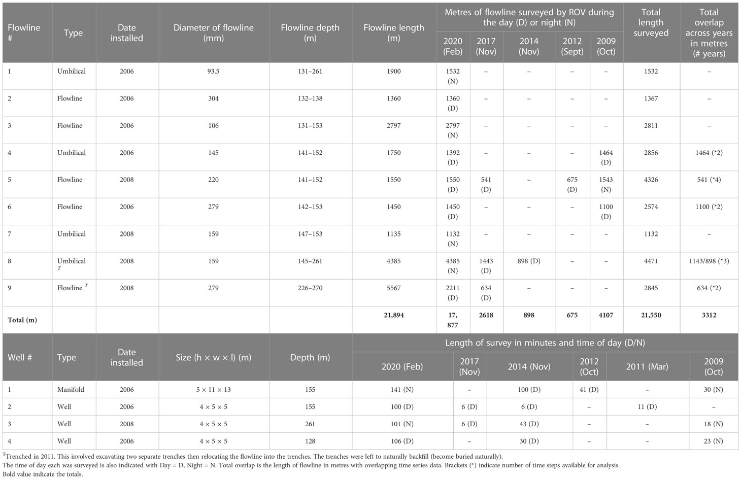
Table 1 Length of flowline assessed (m) for each asset and year, and the age, size, timing and length of ROV survey (minutes) of the manifold and wells studied.
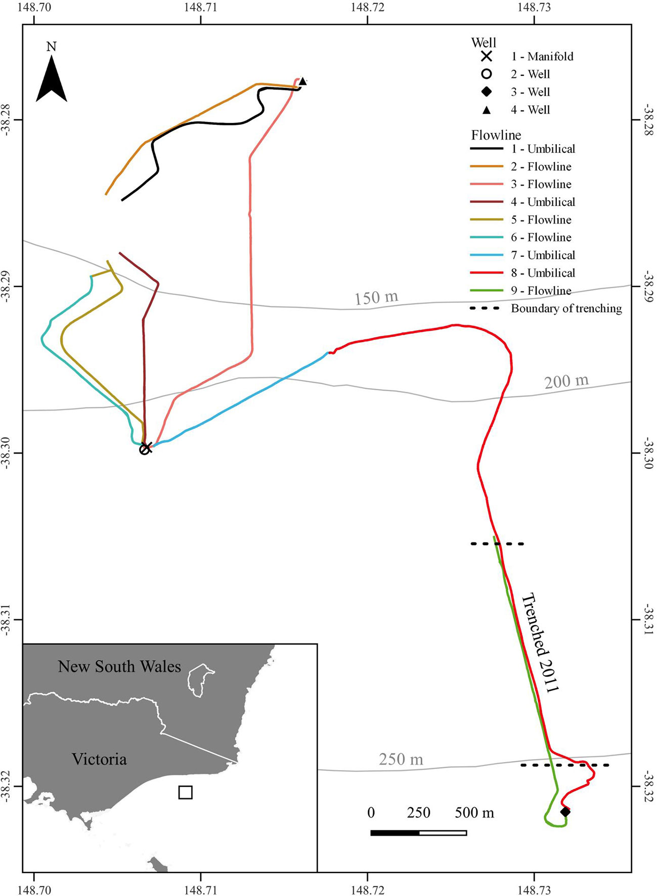
Figure 1 Location of studied offshore field and assets investigated in this study.
2.2. ROV video analyses
The purpose-built software program, TransectMeasure (SeaGIS, 2020), was used to record broad classifications of benthic habitat on structures using an adaptation of the CATAMI (Collaborative and Annotation Tools for Analysis of Marine Imagery; Althaus et al., 2015) classification scheme. An additional specialized program, EventMeasure Stereo (SeaGIS, 2020), was used to annotate mobile fauna from ROV video. Both software programs were designed specifically to allow fast, and efficient analysis of biological information from video sequences and have been used previously to analyze ROV videos (McLean et al., 2017; McLean et al., 2018; Bond et al., 2018a; McLean et al., 2019; ).
2.2.1. ROV video analysis of flowlines
In total, ~22 km of flowline had ROV video imagery that was suitable for analysis across the years (Table 1), with most of this collected in 2020 (17.8 km – single data collection across all flowlines). Imagery was deemed suitable for analysis if the ROV video provided a good view of the flowline, without obstruction or being focused on a small area only (see McLean et al., 2020b). Prior to 2020, standard definition imagery was collected from port, center and starboard cameras providing an oblique and often grainy view of each flowline, however, only sections of flowlines were sometimes surveyed (not the entire flowline) (Table 1). In contrast, the 2020 survey collected high-resolution downfacing video using a CathX system.
The abundance of all fish, mobile invertebrates, and other animals (e.g. seals) encountered along each flowline were recorded and identified to lowest taxonomic rank. Several fish could not be consistently or reliably identified to species level and were therefore recorded to the next lowest taxonomic level possible which was often genus or family (e.g. Pseudophycis spp. and Helicolenus spp.). Analyst’s cross checked their identifications to reduce the chance of interobserver biases. Unlike previous surveys in north-west Australia (McLean et al., 2017), no fish were observed to swim along in front of the ROV, leaving the field of view (FOV) and as such the chances of recounting any individuals was deemed low for flowlines. Fish length (snout to tail fork) was estimated in size class categories <20, 20–30, 30–40, 40–50, >50 cm, using the known diameter of each flowline (Table 1) as a guide. Consistent ROV fly heights and field of views within surveys enabled estimated size categories to be determined when flowlines were not visible when trenched.
A virtual quadrat measuring ~4 m2 (~150 cm x ~270 cm, derived from the relatively constant ROV altitude) was placed on a freeze-framed image taken every 50 m along flowlines and spanned the flowline and seafloor to either side. Within each quadrat, a 20-point grid was allocated, and biota identified to the lowest taxonomic resolution possible within the grid. Benthos and substrate were categorized using quadrats and a modified CATAMI classification schema (Althaus et al., 2015) that included black/octocorals, encrusting sponges, massive sponges, Actiniaria (anemones), bryozoans, ascidians, biofilm, rubble, burrows, shells, pebble/gravel, sand, open water, fish and scores for unidentifiable and not useable data as an indication of image quality. Biofilm refers to flowlines that appear somewhat bare but have a thin layer of biota, likely a mix of cnidaria and bryozoans. In addition to benthic biota, the density of burrows in the sediment immediately adjacent to the flowline (within the quadrat), indicating infauna presence, were assessed as low (burrows present in <5% of seafloor within quadrat), medium (5–25%) and dense (>25%) and the size of each burrow estimated as <2, 2–8 cm and >8 cm, using the known size of the flowline as a guide. Benthic community height and density were scored in the FOV of the pipeline at the same location as quadrats to examine potential relationships with fish and invertebrate abundance. For height, this included 0 = none; 1 = low (0–20 cm), 2 = medium (20–40 cm) and 3 = high (>40 cm). Density scores included 0 = none, 1 = sparse (<25% percentage cover for entire FOV), 2 = medium (between 25–75% percent cover for entire FOV), 3 = dense (>75% percent cover for entire FOV). Video quality was also scored at these points; 1 being poor quality, 2 indicating moderate quality, and 3 indicating good quality. The same analyst undertook all benthic assessments to avoid any inter-observer variability.
To examine relationships between fish, benthic biota, and the position of flowlines relative to the seafloor, ‘flowline position’ was scored similarly to McLean et al. (2020b) with 0 = completely buried, 1 = flowline showing but more than halfway buried, 2 = flowline touching the seafloor but making a closed crevice, 3 = underside of flowline not touching the seafloor (spanning), and 4 = flowline >0.5 m above the seafloor. Flowline position was recorded in tandem with every fish observation.
2.2.2. ROV video analysis of wells and the manifold
For analysis of fish and mobile invertebrates on the wells/manifold, each structure was divided into six sections to determine the role of structure position in shaping communities observed. For wells, these sections included: tree cap assembly (top of the well), Christmas tree general (main middle section of the well), flow base (base of the well), seafloor around structure, seafloor beneath structure and water column around structure as described by McLean et al., 2022. The same general locations were identified on the manifold, namely the cap assembly, manifold module, base, seafloor beneath structure and water column around structure. The height of each of these structure sections was similar however the width and length of the manifold was greater resulting in more surface area for benthic habitats, fish and mobile invertebrate communities on this structure (Table 1).
To prevent repeated counts of the same individuals leaving and re-entering the field of view, the conservative measure MaxN (the maximum number of individuals of the same species present in the field of view at one time) was used to estimate relative abundance (Cappo et al., 2007). The length of ROV surveys of each structure varied dramatically across the years (Table 1) from rapid general visual inspections (6 mins) to detailed structural assessments (>100 mins). As a result, a more conservative measure of the ‘maximum MaxN’ observed for the entire well (highest MaxN observed across all sections) for each species was used for temporal comparisons. Therefore abundances are likely conservative.
Benthic habitats on wells/manifold were analyzed by obtaining 10 non-overlapping FOV images per section of the structure (n = 60 total) and randomly allocating 20 points per FOV image. It was not possible to standardize the size of these FOV images due to high variability in ROV movements relative to the wells/manifold, however the point classification enabled the percent cover of each biotic component, identified to the lowest taxonomic resolution, to be quantified.
2.3. Data analyses
2.3.1. Spatial distribution of marine communities
Analyses were conducted to assess whether faunal assemblages differed among flowlines or wells/manifold using the comprehensive 2020 dataset only. For flowlines, fish and mobile invertebrate observations were grouped into 50 m transects, with this distance chosen to provide sufficient replication along each flowline while also capturing spatial variability in communities observed. For wells, too few mobile invertebrate taxa were observed for inclusion in statistical analyses, but these communities are described.
The separate multivariate fish and mobile invertebrate data sets were compared among flowlines in 2020 in PRIMER V7 (Clarke and Gorley, 2015) with the PERMANOVA+ add on (Anderson et al., 2008). Each assemblage was assessed using shade plots to determine the appropriate transformation level (Clarke et al., 2014), which for fish was dispersion weighting by flowline, while the invertebrate data needed no transformation. Dispersion weighting is becoming a commonly used transformation that enables better representation across species and down-weighs spatially clumped species (e.g. fish schools; Clarke et al., 2014). A Bray-Curtis dissimilarity matrix was constructed for each data set (Anderson et al., 2008) using a dummy variable on the factor of Flowline (nine levels, fixed) to include 50 m sections of flowline without taxa.
A canonical analysis of principal coordinates (CAP; Anderson and Robinson, 2003; Anderson and Willis, 2003) was undertaken for both fish and invertebrate datasets to visually examine patterns among flowlines. A leave-one-out allocation test (Anderson and Robinson, 2003) was used to provide a statistical estimate of misclassification error and demonstrate how distinct assemblages were in multivariate space (Anderson and Willis, 2003). Individual species that were likely responsible for any of the observed differences were identified using Pearson correlations of their abundance with the canonical axes. A Pearson correlation of |R| ≥ 0.3 was used as an arbitrary cut-off to display potential relationships between individual species and the CAP axes. These relationships are graphically illustrated through the use of vectors that are superimposed onto the CAP plot made using the R packages ggplot2 (Wickham, 2016) and gridExtra (Auguie, 2017).
Separate analyses were undertaken for those four flowlines with over-lapping temporal data and aimed to assess change in fish and mobile invertebrate assemblages (combined data set) over time. The first analysis was conducted on Flowline 5 and involved assessing ~550 m of the same sections of flowline across four time periods (2009, 2012, 2017, and 2020). Data were visualized using shade plots before applying a dispersion weighted transformation (by flowline; Clarke et al., 2014) and calculating a Bray-Curtis similarity matrix. A repeated measures PERMANOVA with the lowest replication level, ‘Transect’ was conducted to assess change across years (four levels, fixed) and included video quality (Supplementary Table 1) as a covariate, with subsequent pairwise tests used to investigate significant differences. A CAP plot was used to visually assess patterns and differences across years.
The same analysis was undertaken for Umbilical 8 (2014, 2017, 2020). However, transects in 2017 and 2014 were not overlapping due to the surveys being conducted on different flowline sections, thus an additional qualifier was added to the 2020 dataset to match to either 2017 or 2014 (<1500 m section or >1500 m section). We combined data obtained from Umbilical 4 and Flowline 6, as they were surveyed at the same time (2009 and 2020) and included a second factor ‘Flowline’ into the PERMANOVA analysis. Flowline 9 had two time points (2017 and 2020) and was analyzed separately.
Analyses of fish communities observed on wells/manifold used the same methods described above for the 2020 data using a dispersion-weighted Bray-Curtis similarity matrix, but according to the factors Structure (4 levels, fixed) and Section (6 levels, fixed). Due to differences in the time of survey, duration of survey (Table 1) and video quality (Supplementary Table 1), well and manifold temporal data were only able to be examined heuristically with data presented in descriptive figures rather than undergoing formal statistical analysis. This included metric multidimensional scaling (mMDS) to visually represent patterns of fish communities among years and depths (Clarke et al., 2014).
2.3.2. Influence of survey-specific, environmental, and benthic variables on fish and mobile invertebrate communities
Relationships between the fish and mobile invertebrate Bray-Curtis dissimilarity (described above) and normalized benthic habitat, flowline position, depth and distance to the nearest structure variables (n = 11) were explored using distance-based linear models (DISTLM) and distance-based redundancy analysis (dbRDA; McArdle and Anderson, 2001; Anderson et al., 2008) in the PRIMER-E statistical software package. Variables were checked for correlations using draftsmen plots, with percent cover of shell/pebble strongly negatively correlated with percent cover of sand (-0.95). Thus, percent cover of shell/pebble was excluded from analyses. A stepwise selection procedure was used in which the contribution of each variable was assessed for statistical significance using marginal tests (from 9999 permutations) and percentage contribution of each set of variables (Anderson et al., 2008). A dbRDA plot was produced using the R packages ggplot2 (Wickham, 2016) and gridExtra (Auguie, 2017) for visualizing relationships between the assemblages and associated variables.
The influence of epibenthic community percent cover and complexity, and of flowline position on fish and mobile invertebrate diversity, total abundance, abundance of ubiquitous (species with <80% zero samples and those identified in CAP) and commercial fishery species were investigated using generalized additive models (GAMs; Hastie and Tibshirani, 1986). Because of strong collinearity, a full subsets approach was used to fit all combinations of predictor variables up to a maximum of three (to prevent over-fitting and ensure models remained ecologically interpretable). Time of day was treated as a circular variable using the function (bs=‘cc’) in mgcv (Wood, 2011). Models containing combinations of variables with correlations >0.28 were excluded. The best model had the fewest variables (most parsimonious) and was the one with lowest Akaike information criterion (AIC). Best models were also within two AIC units of the lowest AIC value (Burnham and Anderson, 2003; Symonds and Moussalli, 2011).
As recommended in the literature (O’Hara and Kotze, 2010), we used untransformed abundance metrics as our response variables. Models were fitted using a Tweedie error distribution (Tweedie, 1984). A Tweedie model is an extension of a compound Poisson model derived from the stochastic process where a gamma distribution is used for the counted or measured objects (i.e. number of fishes) and has an advantage over delta-type two-step models by handling the zero data in a unified way. All GAM modelling and plots were performed using the R language for statistical computing (R Development Core Team, 2019) with the package mgcv (Wood, 2011) and ggplot2 (Wickham, 2016), and based on the approach by Fisher et al. (2018).
Linear regression models were produced to understand if the cover of colonizing invertebrates (summed cover of ascidians, bryozoans, sponges, and black/octocorals) correlated with well/manifold age and depth. Benthic habitat data from wells/manifold in this study were combined with those reported by McLean et al. (2019) to see if relationships held with those previously documented in north-west Australia. Analysis was undertaken using the R language for statistical computing (R Development Core Team, 2019) and plotted with ggplot2 (Wickham, 2016).
3. Results
3.1. Overview of species richness and abundance
A total of 10,343 individual animals were observed and comprised 69 taxa including bony and cartilaginous fishes, mammals, and invertebrates (Supplementary Tables 2, 3; Supplementary Figures 1, 2). There were 16 species observed of commercial fisheries interest, and three species of conservation value including, handfish (Brachionichthyidae spp.), stingaree (Urolophus spp.), and foxfish (Bodianus frenchii); although these are tentative identifications unable to be verified from the imagery obtained. Australian fur seals (Arctocephalus pusillus doriferus) were observed multiple times along flowlines in 2009, including juvenile males and adult females (Supplementary Data Table 2).
More species of fish were recorded on flowlines (n = 28 species) compared to wells and manifold (n = 19 species). An average of 295 ± 45 individual fish were recorded per km of pipeline. Considering the comprehensive 2020 dataset on its own, 16 species of fish were recorded on the flowlines that were not observed on the wells or manifold, including species closely associated with the benthos e.g. banded cucumberfish (Paraulopus balteatus), ghost flathead (Hoplichthys spp.). Eight species of fish were unique to the wells and manifold which included more mobile, schooling species such as Australian sandpaper fish (Paratrachichthys macleayi) and redfish (Centroberyx affinis). Eight species were observed on both infrastructure types, including commercial fishery species such as ocean perch (Helicolenus spp.), jackass morwong (Nemadactylus macropterus) and pink ling (Genypterus blacodes).
A total of 2,066 individual invertebrates comprised of 32 species were observed on flowline surveys across all survey years (Supplementary Data Table 2). Invertebrate taxa were identified from four phyla, of which Arthropoda and Cnidaria had the highest abundance. A total of 27 individual invertebrates were observed on the wells and manifold across all years and comprised seven taxa (Supplementary Data Table 3). Pancake urchin (Araeosoma thetidis) was the only mobile invertebrate species recorded on both types of infrastructure.
3.2. Extent of burial of flowlines
Using the 2020 data only, forty one percent of flowlines surveyed were classed as ‘buried’. This was most prevalent on Umbilical 7 and 8, and Flowline 9 where 97- 100% was buried. Where flowlines were classified as exposed; 32% of observations were less than 50% exposed, 15% were greater than 50% exposed and 11% were completely exposed and spanning. There were no observations of any flowline with a span of greater than 0.5 m above the substrate.
3.3. Epibenthic cover of flowlines and wells
Using the 2020 data only, epibenthic cover of flowlines was predominantly abiotic, i.e. sand (>80% cover) for all flowlines except flowline 3 which was a mix of sand (49%) and pebble/gravel (50%). The most prevalent biotic cover was ‘biofilm’ accounting for 3% of the total cover. Overall, all sponge classes accounted for only 0.3% of cover. Among all flowlines, most epibenthic communities were encrusting (61–91%; negligible in height), with very few of low (9–39% values) and moderate (0–4%) complexity. Infauna burrows were observed beside all flowlines, generally in low densities; between 9% (Umbilical 7) and 39% (Umbilical 4) sparse coverage (<25% cover).
For surveys prior to 2020, poor video quality had the largest impact on benthic assessments because it affected our ability to identify epibenthic organisms. As such, large amounts (49%) of historic imagery was classed as either “unidentifiable” (biota too blurry to identify; 20.3%), “not useable” (biota/flowlines not visible; 7.9%) or “open water” (where the ROV view was at an oblique angle, causing some quadrat points to be placed in the water column; 21.5%) (Figure 2), thus, further analyses on these biota metrics was not undertaken. Sand was the dominant habitat scored on flowlines through the time series, but an overall increase in biofilm was also observed among flowlines over time.
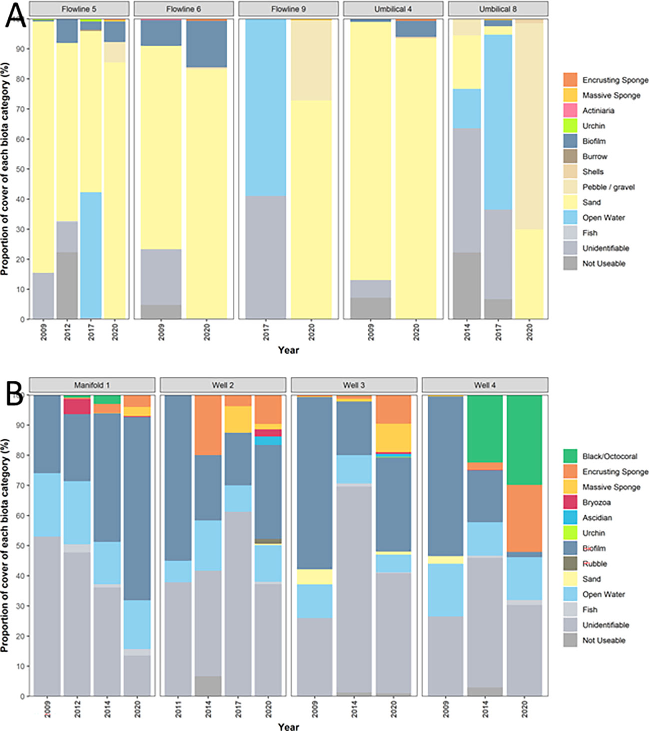
Figure 2 Percentage cover of each benthic biota grouping observed on (A) comparable sections of flowline between 2009 and 2020 and (B) wells and manifolds between 2009 and 2020.
Similar to historic epibenthic habitat classifications of flowlines, a substantial amount (58%) of habitat classifications on wells and the manifold for all years were classed as either “unidentifiable” (37%; video too blurry to identify), “not useable” (0.7%; benthos and flowlines not visible), “fish” (0.9%; where a quadrat point has landed on a fish and the underlying benthos cannot be identified), or “open water” (12%; video where the quadrat point is in the water column). Biofilm was the most common class of biota able to be scored, making up 32% of all classifications (Figure 2). Other types of biotas that were observed in lower densities included sponges (8%; encrusting and massive), black/octocorals (6%) and bryozoans (0.5%). A greater cover of black/octocorals and massive sponge classes were observed in 2020 compared to previous years, although whether this is a true increase rather than a product of improved visibility is not known.
Epibenthic cover was predominantly biotic for all wells and dominated by biofilm for the manifold (61%), Well 2 (31%) and Well 3 (31%). Well 4 had a comparatively high proportion of black/octocorals (22%) and encrusting sponge communities (22%; Figure 2). Black/octocorals, bryozoans and ascidians were not observed on flowlines (Figure 2).
A linear regression of total percent cover of colonizing epibenthic communities on wells and the manifold sampled for this study and reported by McLean et al. (2019) showed weak positive correlation with well and manifold age, suggesting an increase in invertebrate epibiota with increasing time in-situ (Figure 3). The addition of samples from this study reduced the R2 reported by McLean et al. (2019) from 0.43 to 0.29 (Figure 3), noting that McLean et al. (2019) reported on tropical fish assemblages which may exhibit different patterns to those in temperate ecosystems such as those surveyed here. A stronger negative correlation existed between the depth of the well or manifold and the total cover of epibenthos (Figure 3). Similarly, adding samples from this study to the model, reduced the R2 reported by McLean et al. (2019) from 0.74 to 0.57.
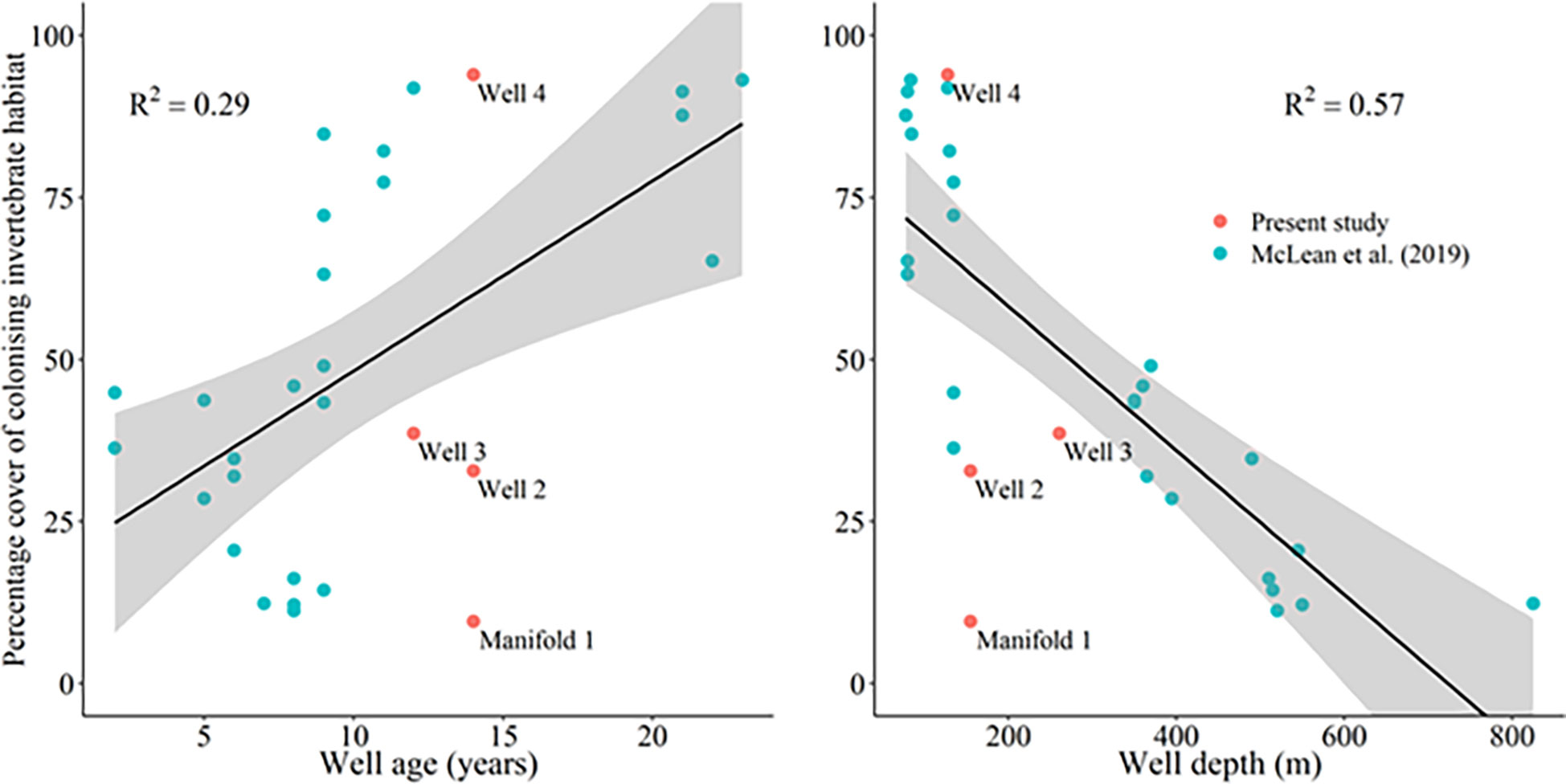
Figure 3 Linear regression of the percent cover of colonising invertebrates against wellhead age and wellhead depth. Shaded regions represent the 95% confidence interval. Samples are presented with those recorded by McLean et al. (2019) which reflect fish communities around wells on the north-west shelf of Australia.
3.4. Fish communities observed along flowlines in 2020
Across the 17.8 km of flowlines assessed in 2020, 5,697 individual fish were identified from 24 taxa equating to a relative abundance of 295 ± 45 individual fish per kilometer (Supplementary Table 4). The most abundant species were also the most ubiquitous (>80% of the observations) and included: Parapercis sp2 (species complex, not including P. allporti); ocean perch (Helicolenus spp.); slender sandburrower (Creedia haswelli); barred grubfish (Parapercis allporti); banded cucumberfish (Paraulopus balteatus); and trevally (Carangidae spp.). Six commercial fishery species were observed along flowlines in 2020 including the aforementioned Carangidae spp. and Helicolenus spp., along with blue grenadier (Macruronus novaezelandiae), jackass morwong (Nemadactylus macropterus), pink ling (Genypterus blacodes), tiger flathead (Platycephalus richardsoni). The relative abundance of commercial fishery species across the flowlines varied, ranging from 0.4–79.1 individuals/km, with Flowline 5 having the highest, mainly comprised of Helicolenus spp. Species of ecological interest included the rarely seen broad duckbill (Enigmapercis reducta) and handfish (anglerfish) within the family Brachionichthyidae. The majority of fish species observed on flowlines were <20 cm in size (snout to tail fork) with frequency substantially declining with increasing size classes (Supplementary Figure 3). Commercial fishery species accounted for 83% of all length observations over 20 cm. For commercial fishery species, 98% of length estimates in the <20 cm class were of Helicolenus spp. (Supplementary Figure 3).
Spatial distribution of total abundance and fish species richness along flowlines (Figure 4) in addition to the abundance distribution of ubiquitous species (Figure 4) show some patterns according to positions along flowlines. Individual species show affinity to particular sections of flowline. Parapercis allporti and C. haswelli were present in higher abundance in northern sections of flowlines, compared to flounder (Bothidae spp.) and Parapercis sp2 which had high abundance at the southern, deeper sections of Umbilical 8 and Flowline 9 (Figure 4).
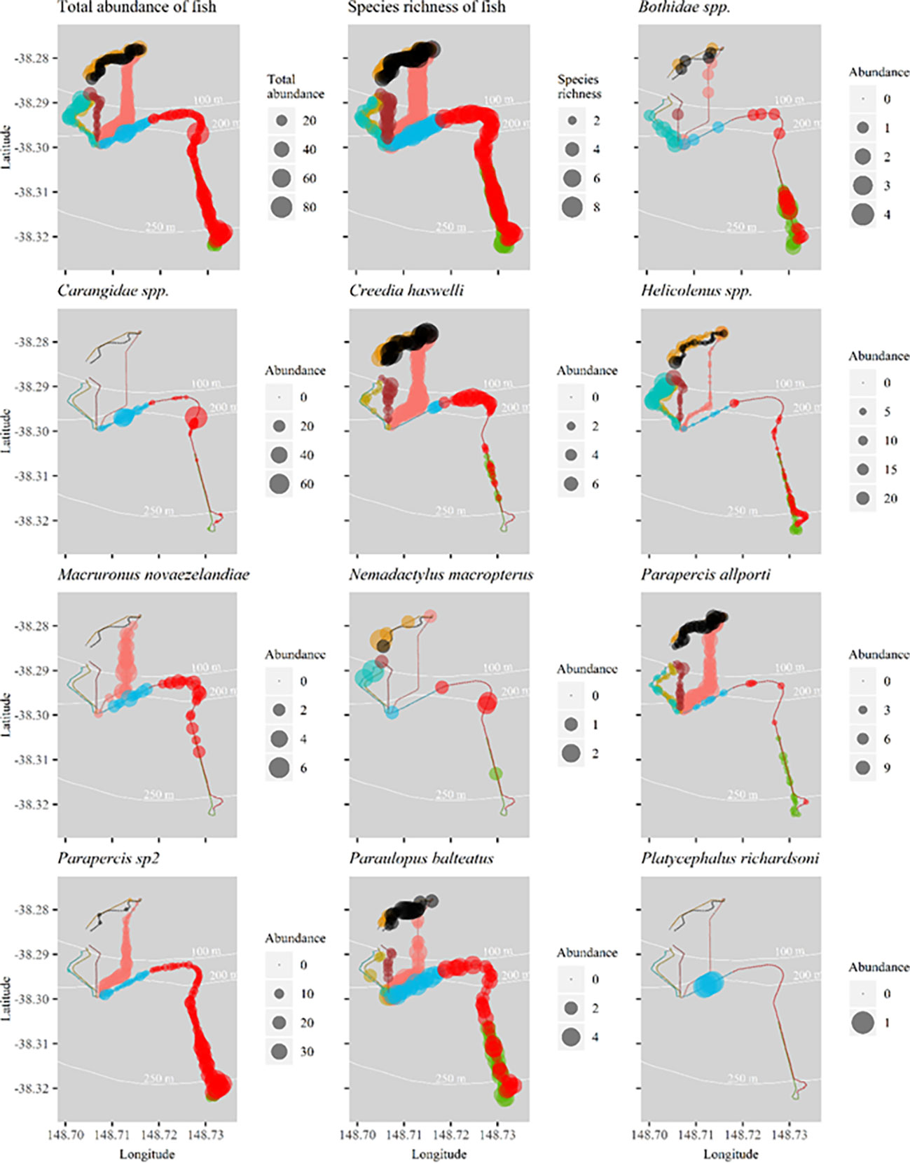
Figure 4 Spatial distribution of total abundance and species richness of fish, and the abundance of key species of fish per transect along flowlines surveyed in 2020. Abundance bubble sizes reflect exact abundance per transect, and therefore bubble size may be larger or smaller than those shown in the legend’s categories. Flowline numbers are indicated in Figure 1.
3.4.1. Influence of survey-specific, environmental, and benthic variables on fish communities observed in 2020
Fish assemblages differed across flowlines in 2020 (Pseudo-F = 25.78, P = 0.001), with all flowline pairs significantly different (t > 1.5, P <0.05; Supplementary Table 5). Fish assemblages also showed distinct clusters on each flowline, particularly for Umbilical 1, Flowline 3, Umbilical 7 and Umbilical 8 (CAP analysis p < 0.01; Figure 5). This distinction between the seven flowlines was illustrated by an overall CAP leave-one-out allocation success rate of 67%. Fish species associated with Flowline 3 included barred grubfish (P. allporti), slender sandburrower (C. haswelli), cocky gurnard (L. modesta), and red cod (Pseudophycis spp.), while the whiptail (Coelorinchus spp.) was correlated with Umbilical 8 (Figure 5). Blue grenadier (M. novaezelandiae) had high abundance at both Flowline 3 and Umbilical 7. While Parapercis sp2 also had high abundances at Flowline 3 and Umbilical 8. Ocean perch (Helicolenus spp.) had the highest abundance on Flowline 6 (Figure 4).
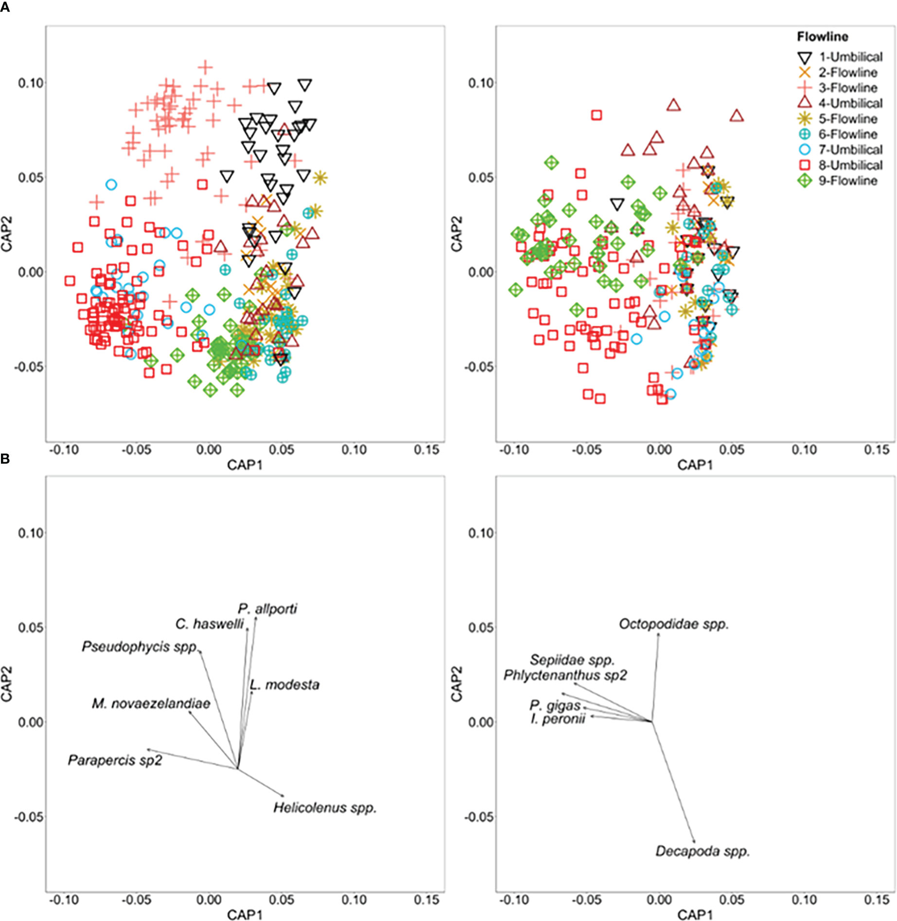
Figure 5 (A) A Canonical analysis of principal coordinates (CAP) ordination based on Bray-Curtis dissimilarities for 1) (Top left) multivariate fish abundance on flowlines and 2) (Top right) mobile invertebrate abundance on flowlines, showing the first two (out of m = 10) axes. Each point represents the assemblage structure (all species) within each 50 m transect of each flowline in relation to the other locations (similarity), with points that are closer together more similar than those further apart. (B) Pearson correlations (|R| ≥ 0.3) for species are displayed as vectors with the length and direction of these vectors representing the strength and direction (relative to the data cloud (A)) of this species association.
Flowline position, depth, percent cover of sand, percent of biofilm on flowlines, and burrow density, all had a significant relationship with the variation in the fish assemblage data cloud when considered alone (p < 0.01). Flowline position explained the greatest amount of variation in the fish relative abundance data cloud at 12%. The variables that reduced the value of AICc the most after fitting flowline position, in the stepwise additive model, were depth (10%, cumulative = 22%), percent cover of sand (3%, cumulative = 25%) and biofilm on flowlines (1%, cumulative = 27%). All of the conditional tests associated with each of these sequential additions were statistically significant (p < 0.05). The best solution contained the five stated variables, flowline position, depth, percent cover of sand, percent of biofilm on flowlines and burrow density and explained 27% of the variation in the fish relative abundance data cloud (Figure 6). The first two dbRDA axes captured 86.4% of the variability in the fitted model and 23.6% of the total variation in the data cloud (Figure 6). The grubfish (Parapercis sp2) and whiptail (Coelorinchus spp.) showed similar correlations to increasing depth, while slender sandburrower (C. haswelli), red cod (Pseudophycis spp.) and blue grenadier (M. novaezelandiae), were more strongly correlated with sand coverage (Figure 6).
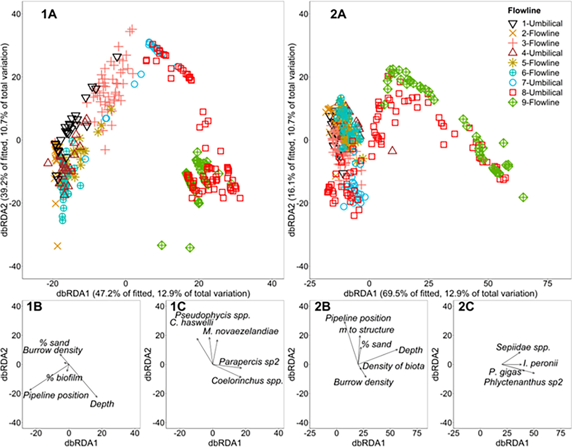
Figure 6 (A) Distance-based redundancy analysis (dbRDA) displaying the relationship between the most important explanatory variables (depth, flowline position, % biofilm on flowline, % sand and burrow density) for 1) (Top left) multivariate fish abundance on flowlines and 2) (Top right) mobile invertebrate abundance on flowlines. (B) Vectors indicate the direction of the relationship with the explanatory variables and their length indicates the strength of their effect on fish abundance. (C) Species with a Pearson correlation of |R| ≥ 0.4 to either axis is displayed as vectors indicating the strength and direction (relative to the data cloud (A) and variables (B)) of their association.
Univariate GAMs were produced for total abundance and fish species richness, as well as the abundance of those species identified in the CAP (Figure 5), species with >80% non-zero samples, and commercial fishery species. No GAM was produced for commercially targeted N. macropterus, M. novaezelandiae, and Platycephalus richardsoni due to low abundances (n = 20, n = 104, and n = 4, respectively).
Percent cover of biofilm was present in the top model for total abundance, species richness, C. haswelli, Parapercis allporti, Parapercis sp2, Paraulopus balteatus, Pseudophycis spp., and Helicolenus spp. (Table 2). Total abundance and the abundance of Helicolenus spp. increased with higher percent cover of biofilm compared to species richness, and abundance of C. haswelli, Parapercis allporti, Parapercis sp2, Pseudophycis spp., and P. balteatus, which generally decreased with increasing percent cover of biofilm (Supplementary Figure 4). Time of day was also included with biofilm in the top models for total abundance and abundance of C. haswelli, P. allporti, Parapercis sp2, and P. balteatus (Table 2). Total abundance and the abundance of Parapercis sp2, and P. balteatus were highest during the night and into sunrise, compared to the abundance of C. haswelli and P. allporti which peaked in abundance at sunset and into night (Figure 7). P. balteatus also showed a pulse in abundance at midday, but abundance peaked at night (Figure 7).
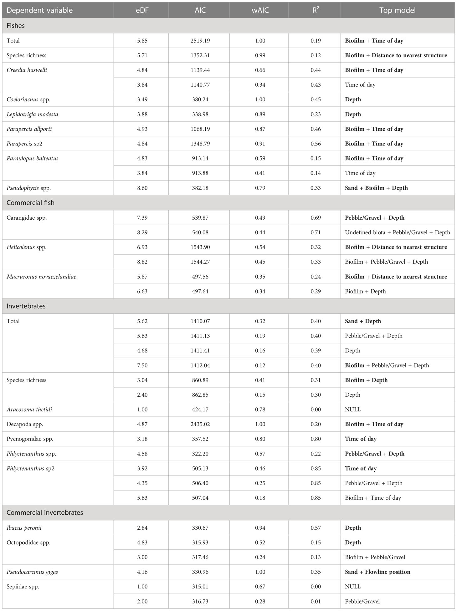
Table 2 Generalised additive models (GAMs) for predicting total abundance and species richness of fish and mobile invertebrates, and the abundance of key species and commercial species along flowlines within 2 AIC of the top model. The best model is indicated in bold.
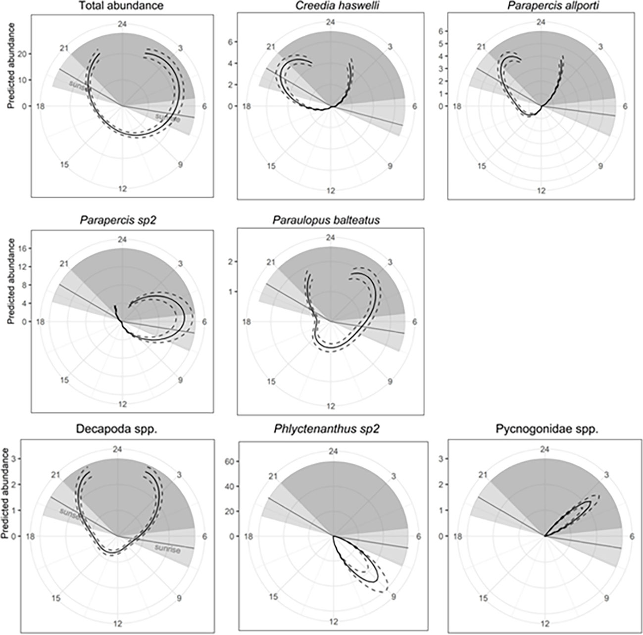
Figure 7 Predicted fish and mobile invertebrate abundance per transect as a function of time of day for all fish (total abundance), common and commercial fishery species plotted over a 24 hour ‘clockface’. Solid lines indicate fitted GAM curves and dashed lines represent ±2×SE of predicts. Light grey shading is the crepuscular period defined as one hour either side of sunset and sunrise. The dark grey shading is night, beginning one hour after sunset and finishing one hour before sunrise. Gaps in the curve indicate the time of the day where no sampling occurred. GAM was circular for available data only, therefore predicted abundance is equal at both ends of the curved displayed.
Depth was the only variable in the top models for Coelorinchus spp. and L. modesta and included in the top models for Pseudophycis spp. and Carangidae spp. (Table 2). Abundance of L. modesta and Pseudophycis spp. decreased with increasing depth, compared to Coelorinchus spp. which increased with depth (Figure 7). Carangidae spp. peaked in abundance at 140 m and at 260 m water depth (Supplementary Figure 4). Distance to nearest structure was included in models for species richness and Helicolenus spp. (Table 2). Species richness peaked at approximately 750 m from structures and was lowest for transects close to structures and those >1500 m away (Supplementary Figure 4). Helicolenus spp. decreased in abundance with increasing distance from structures (Supplementary Figure 4). The percent cover of pebble/gravel was included in the top model for Carangidae spp. only (Table 2) and showed highest predicted abundance at approximately 40% pebble/gravel and lowest predicted abundance when pebble/gravel was not present (Supplementary Figure 4).
3.5. Mobile invertebrate communities observed along flowlines in 2020
For the 2020 survey, a total of 1,466 mobile invertebrates from 31 taxa were identified, equating to 71 ± 12 individuals/km of flowline (Supplementary Table 2). Mobile invertebrate taxa were identified from four phyla with Arthropoda and Cnidaria dominating the assemblage, in particular, hermit crabs (n = 443) and anemone sp2 (n = 328). Invertebrates of commercial importance included the Tasmanian giant crab (Pseudocarcinus gigas, n = 47), cuttlefish (Sepiidae spp., n = 93), octopus (Octopodidae spp., n = 44), arrow squid (Nototodarus gouldi, n = 1), and Balmain bug (Ibacus peronii, n = 35).
Total abundance and species richness of mobile invertebrates varied spatially, with higher abundance and diversity below 200 m depth (Figure 8). Individual species show affinity to particular sections of flowline. For example, I. peronii, P. gigas, anemone sp2, Phlyctenanthus sp2 and Sepiidae spp. were observed in comparatively high abundance at the southern section of Umbilical 8 and Flowline 9 (Figure 8).
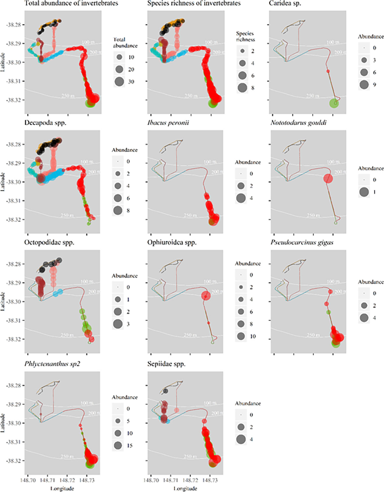
Figure 8 Spatial distribution of total abundance (top left), species richness (top right) and the abundance of common mobile invertebrate species per transect along flowlines surveyed in 2020. Abundance bubble sizes reflect exact abundance per 50m transect, and therefore bubble size may be larger or smaller than those shown in the legend’s categories. Refer to Figure 1 for flowline names.
3.5.1. Influence of survey-specific, environmental, and benthic variables on mobile invertebrate communities observed in 2020
Mobile invertebrate assemblages differed across flowlines (Pseudo-F = 11.92; P = 0.001), however, six pairs of flowlines showed no significant difference, with three pairs involving Flowline 6 (Supplementary Table 5). A CAP analysis, constrained by ‘flowline’, shows some separation between flowlines, particularly for Umbilical 8 and Flowline 9 (p <0.01; Figure 5). There was generally a poor level of distinction between the seven flowlines as illustrated by an overall CAP leave-one-out allocation success rate of only 35%. Mobile invertebrate species associated with the deeper, more southern flowlines Umbilical 8, and Flowline 9, included cuttlefish (Sepiidae spp.), anemone sp2 (Phlyctenanthus sp2), Tasmanian giant crab (P. gigas), and Balmain bug (I. peronii).
Depth, distance to nearest structure, flowline position, burrow density, percent cover of sand and the density of biota all had a significant relationship with the variation in the invertebrate assemblage data cloud when considered alone (all p <0.01). Depth explained the greatest amount of variation in the mobile invertebrate relative abundance data cloud at 17%. The variables that increased the value of AICc the most after fitting depth, in the stepwise additive model, were distance to nearest structure (5%, cumulative = 22%), flowline position (4%, cumulative = 27%) and burrow density (1%, cumulative = 28%). All of the conditional tests associated with each of these sequential additions were statistically significant (p <0.05). The best solution contained the aforementioned six variables and explained 28% of the variation in the mobile invertebrate relative abundance data cloud (Figures 5, 6).
Univariate GAMs were produced for the total abundance and species richness of mobile invertebrates, as well as the abundance of those species identified in the CAP (Figure 5), species with >80% non-zero samples, and commercial fishery species. As evident from spatial distribution plots (Figure 8), depth was an important predictor variable and present in the top model for total abundance, species richness, anemones (Phlyctenanthus spp), Balmain bug (I. peronii) and octopus (Octopodidae spp.) (Table 2). Models including depth showed increasing species richness and abundances of mobile invertebrates with increasing depth. Octopus (Octopodidae spp.) also showed a peak in abundance in shallower depths. Time of day was included in the top model for hermit crabs (Decapoda spp.), sea spiders (Pycnogonidae spp.), and anemones (Phlyctenanthus sp2) (Table 2). Hermit crabs (Decapoda spp.) displayed higher abundances at night, anemones (Phlyctenanthus sp2) peaked after sunrise, and sea spiders (Pycnogonidae spp.) peaked during the night (Figure 7). Species richness and Decapoda spp. included percent cover of biofilm in their top models (Table 2) and both increased with increasing percent cover (Supplementary Figure 5). Percent cover of sand and flowline position were the only two variables in the top model for P. gigas (Table 2) with a higher abundance when the flowline is buried by sand.
3.6. A comparison of marine communities observed on flowlines from 2009 - 2020
Prior to 2020, the majority of ROV imagery of flowlines (75% of transects) was of poor video quality, while 25% was of moderate quality. In contrast, 100% of 2020 ROV imagery was of good quality, although the downward nature did make identification of some fish species difficult (Supplementary Table 1). Only one commercial fish species was observed in historical video imagery (2014) but not also observed in 2020; the gemfish (Rexea solandri, n = 3). All others that were observed in historical imagery were observed in 2020 (Supplementary Table 2).
For fish and mobile invertebrates, the same sections of five flowlines were assessed over time enabling evaluation of change to these communities (Table 1; Flowline 5, Flowline 6, Umbilical 4, Umbilical 8, Flowline 9). For these repeated measures assessments, the ‘video quality’ covariable had a significant impact on assemblages on all flowlines (Table 3). Even considering large differences in video quality, fish, and mobile invertebrate assemblages along two flowlines (Flowline 5 and Umbilical 8) changed across years (Table 3). Assemblages observed in 2020 had higher abundance and species richness than those in previous years for Umbilical 8, while Flowline 5 only had higher abundance for fish in 2020 (Figure 9), but not for species richness or for mobile invertebrate abundance or richness, with these remaining relatively constant over time (Figure 9).
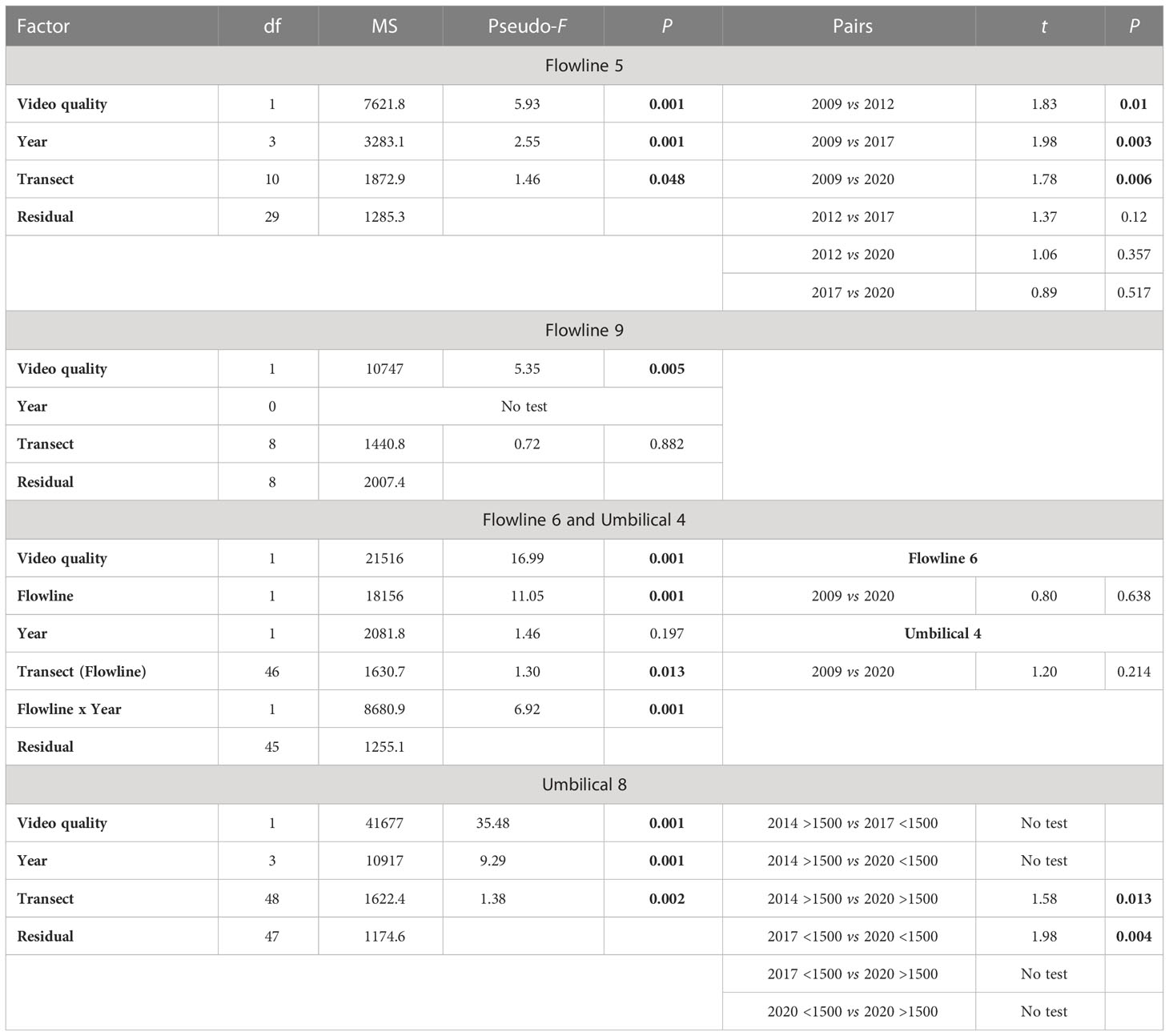
Table 3 Repeated measures PERMANOVA results and pairwise test results for historic flowline comparison on the fish and mobile invertebrate assemblage combined, using a video quality metric as a covariate. Significant values are shown in bold. Unique permutations varied from 992–999.
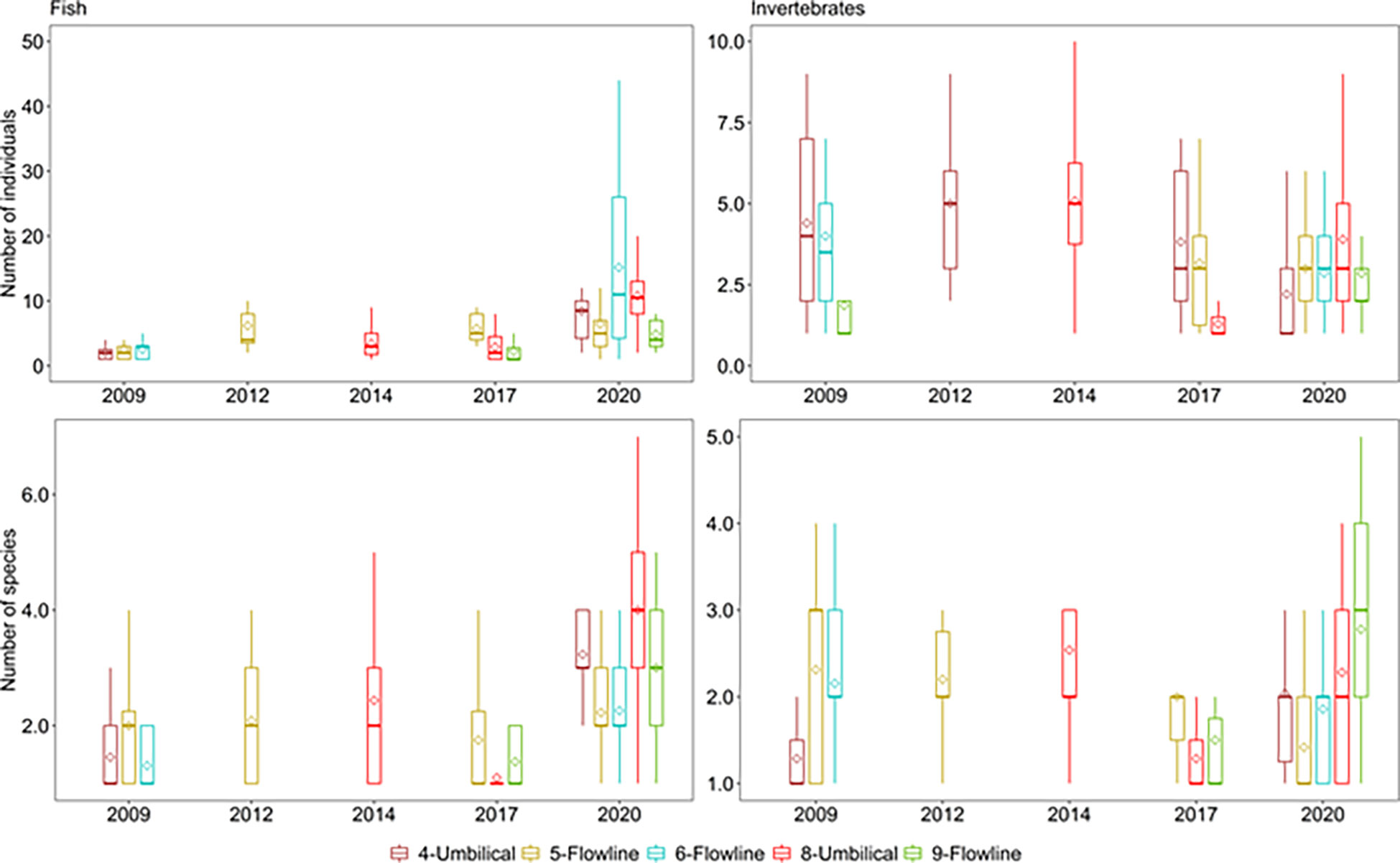
Figure 9 Comparisons of the mean (◊) and median (|) number of fish species (left) and mobile invertebrates (right) and individuals per 50 m transect on the flowlines across years surveyed. The upper and lower hinges represent the first and third quartiles (the 25 and 75 percentiles). The whiskers extend from the hinge to the largest and smallest value, but no further than 1.5 × the interquartile range.
Separation of assemblages by Year is evident for both Flowline 5 and Umbilical 8 (Figure 10), with a moderate level of distinction between years for Flowline 5 (67% allocation success rate) and a good level for Umbilical 8 (89% allocation success rate). Species correlated with the CAP axes for Flowline 5 were distinct for each year with Australian fur seal (A. pusillus doriferus), pancake urchin (A. thetidis), and P. balteatus correlated with 2009, Decapoda spp. and P. allporti correlated with 2012, Octopodidae spp. with 2017, and Helicolenus spp. with 2020. While for Umbilical 8, Sepiidae spp. were correlated with 2014, and A. thetidis with 2017. Multiple species were correlated with 2020 including Decapoda spp., squat lobsters (Galathea australiensis), Coelorinchus spp., Phlyctenanthus spp., and Parapercis sp2 for the section >1500 m along the flowline that matched with the area surveyed in 2014 and Pseudophycis spp., M. novaezelandiae, Pycnogonidae spp., and C. haswelli, in the section <1500 m along the flowline that matched with 2017.
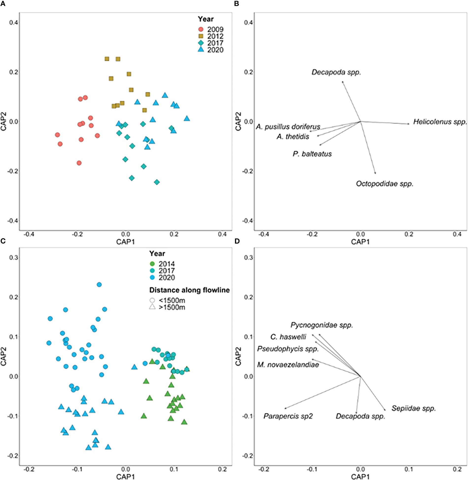
Figure 10 Canonical analysis of principal coordinates (CAP) ordination based on Bray-Curtis dissimilarities for multivariate fish and invertebrate abundance on the (A) Flowline 5 and (C) Umbilical 8 flowlines. Each point represents the assemblage structure (all species) within each 50 m transect of each flowline in relation to the other locations (similarity), with points that are closer together more similar than those further apart. Pearson correlations (|R| ≥ 0.4) are displayed as vectors for (B) Flowline 5 and (D) Umbilical 8 flowlines with the length and direction of vectors representing the strength and direction, respectively, of the relationship.
3.7. Marine communities around the manifold and wells
3.7.1. Fish and mobile invertebrate communities on the manifold and wells in 2020
For 2020, over 787 individuals were identified from 16 fish species (Supplementary Table 3) were observed. An estimated additional 2,517 additional individual fish were noted but not able to be identified to species level, primarily due to the angle of the imagery (not reported on further). Eight of these species were unique to wells and not encountered on flowlines. Wells 2- 4 had high abundances of Australian sandpaper fish (P. macleayi) while the manifold had a greater abundance of redbait (Emmelichthys nitidus) and jackass morwong (N. macropterus). A range of perch species were also abundant on wells e.g. splendid perch (Callanthias australis) and butterfly perch (Caesioperca spp.). Six species of commercial importance were observed including redfish (Centroberyx affinis), redbait (E. nitidus), pink ling (Genypterus blacodes), ocean perch (Helicolenus spp.), striped trumpeter (Latris lineata) and N. macropterus.
MaxN is a conservative and relative abundance metric which cannot be converted into an absolute density as done for flowline. However, the total relative abundance of fish can be expressed relative to the surface area of the structure if each structure is considered as basic cuboid. The surface area of Well 2 – 4 is 105 m2 and the surface area of the manifold is 365.19 m2. The total relative abundance of identified fish species per m2 ranged from 0.79 fish m-2 at Well 2 to 1.90 fish m-2 at Well 4.
Across all wells and the manifold, the tree cap assembly had the highest abundance of fish taxa followed by the Christmas tree and the flow base. The tree cap and Christmas tree also had the highest diversity at 11 and 12 species, respectively, compared to 10 for the flow base and four for other areas. The majority of fish species for which length estimates were made on wells were in the 20-30 cm size range, with 30% of these commercial fishery species. Helicolenus spp. were mostly 30-40 cm in size and N. macropterus 40-50 cm (Supplementary Figure 3).
For 2020 observations, fish communities differed across wells and across sections of each wells (p = 0.001; Supplementary Table 5). All wells possessed distinct fish communities (p = <0.04) with the exception of Well 2 and Well 4 (p = 0.06; Supplementary Table 5). Callanthias australis was associated with Well 4 while all other species were correlated with the manifold (Figure 11). There was a good level of distinction between the wells, as illustrated by an overall CAP allocation success rate of 80%, with each group equally distinct (80% success rate per group).
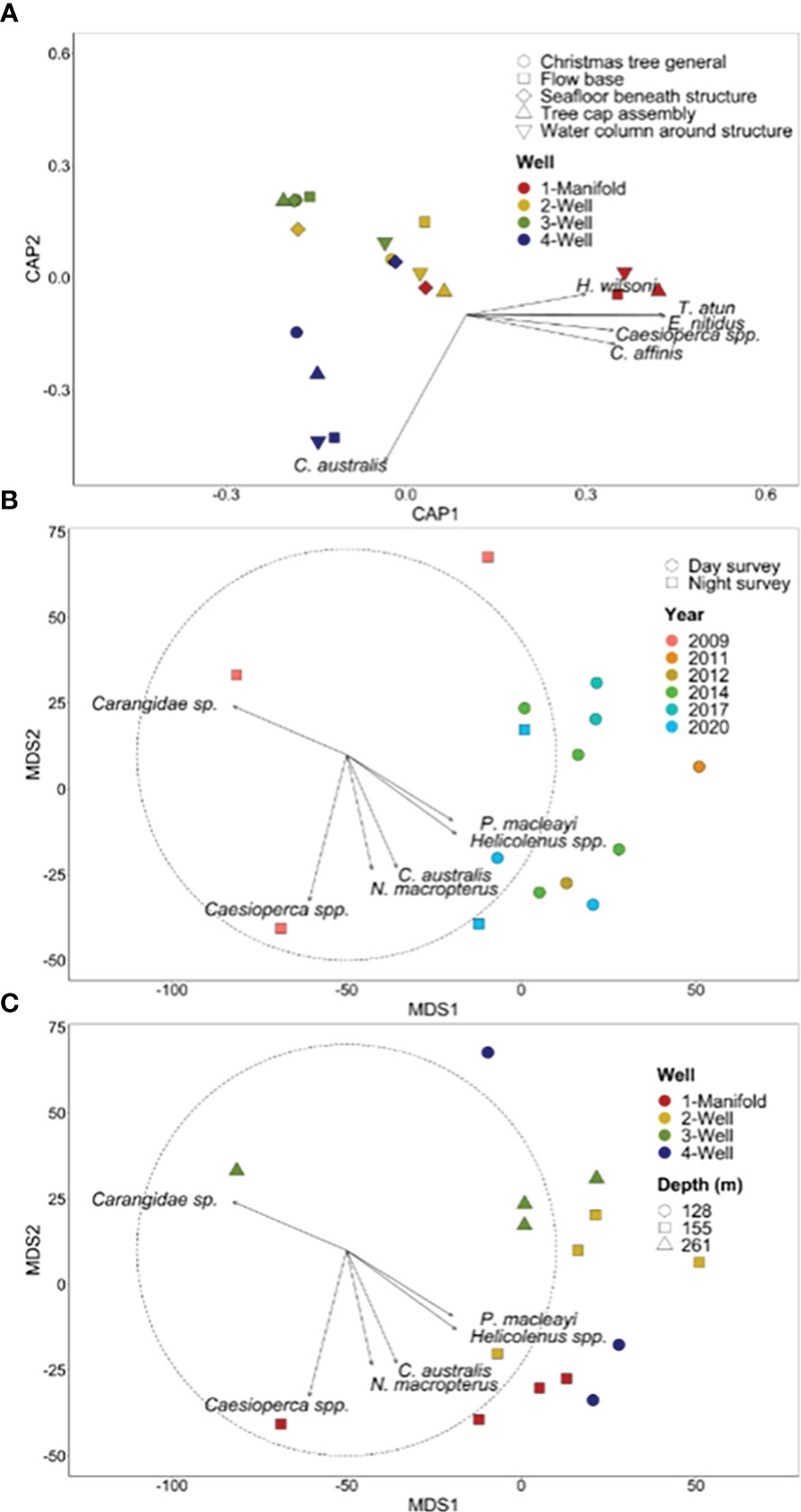
Figure 11 (A) Canonical analysis of principal coordinates (CAP) ordination based on Bray-Curtis dissimilarity for fish species abundance for well assets. Each point represents the assemblage structure (of all species) for each well/manifold in relation to the other locations (similarity), with points that are closer together more similar than those further apart. Species with a Pearson’s correlation of |R| > 0.4 are represented as vectors in an overlay. The length and direction of vectors indicate the strength and direction, respectively, of the relationship. Metric multi-dimensional scaling (mMDS) ordination of all well surveys with plot (B) illustrating patterns among year and time of survey and plot (C) illustrating patterns among depth and well; species with the strongest positive (>0.55) and negative (<−0.55) Pearson’s correlation values are displayed as vectors.
3.7.2. A comparison of marine communities around the manifold and wells across years
A total of 2,196 individual fish from 19 species were observed on the wells across the six surveys spanning 11 years using the conservative measure of ‘maximum MaxN’ for each well (Supplementary Table 3). Fish assemblages were dominated by the Australian sandpaper fish (P. macleayi) which was at least six times more abundant than any other species. Species of ecological interest included the Australian fur seal (A. pusillus doriferus) with one observation in 2009 and the western foxfish B. frenchii.
Comparisons across years for the well and manifold surveys need to be interpreted with caution given the differing time of day sampled, duration of surveys, depth, and size of the structures. Metric multi-dimensional scaling plots show a distinct separation of fish assemblages observed during the first 2009 survey from surveys in later years (Figures 11B, C). Surveys beyond 2009 were characterized by Australian sandpaper fish (P. macleayi) and Helicolenus spp. Two clusters were evident among the years beyond 2009 with one grouping being comprised of Well 2 and Well 3 and the other cluster primarily the manifold and Well 4 (Figure 11B). Callanthias australis (Figure 11A) and N. macropterus (Figure 11C) were strongly associated with the manifold and Well 4.
Total abundance and species richness generally increased across the years at each well, however, the duration of the survey also increases through time with the exception of some short six-minute surveys conducted in 2014 and 2017 (Figure 12). The highest number of species (14) were observed on Well 2 in 2020 whilst the highest number of individuals (650) were observed on the manifold in 2012 which was largely comprised of P. macleayi (Figure 12). Three species P. macleayi, Helicolenus spp. and Pseudophycis spp. were consistently present at all wells and across all years with the exception of the first 2009 survey.
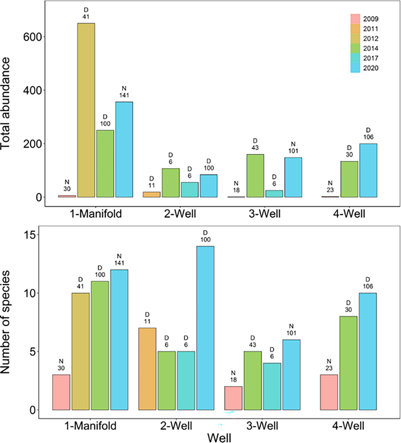
Figure 12 Total abundance (maximum MaxN’s) and number of species of fish sampled for each well survey. Above the bars, the letter ‘D’ indicates a daytime survey whilst ‘N’ indicates a night survey. The number above the bars refers to the duration of the survey in minutes.
4. Discussion
An improved understanding of marine communities associated with oil and gas infrastructure in the Bass Strait region is particularly important given the ecological and socio-economic importance of the region. Industry-collected ROV video provides a unique opportunity to examine marine communities associated with subsea flowlines and wells. While historical ROV video has, in recent years, been used to survey marine communities around infrastructure in Australia’s tropical north-west (e.g. Thomson et al., 2018; Bond et al., 2018a; McLean et al., 2020a; ), only a small handful of published papers exist for the temperate Bass Strait region, one focused on using animal-borne imagery to evaluate infrastructure space use (Arnould et al., 2015), another examining plankton communities around platforms (Neira, 2005) and two recent studies that use historical industry ROV imagery to describe fish and benthic communities on a small number of wells, pipelines and platforms (McLean et al., 2022; Sih et al., 2022). The data for wells presented in McLean et al. (2022) was obtained from the present study and included data for Well 2 and 4 only. Here, we demonstrate the potential utility of industry collected ROV data for documenting biodiversity values of offshore infrastructure.
Using imagery collected by industry gives us a unique opportunity to observe areas that are often difficult and expensive to assess. However, given industry surveys are not specifically designed for scientific data collection, there are naturally issues with standardizing methodology and design to make experimentally robust comparisons. Historical comparisons here are interpreted with caution, given the different video quality, time of day, and duration of surveys. While a generally low diversity of fishes might be expected on poor quality video obtained from historical ROV surveys, the 2020 high-definition imagery was likely also be hindered by the downward-facing camera not capturing species in front of the ROV. As downward facing high-definition imagery is essential for epibenthic communities and invertebrates, a combination of downward and forward-looking HD cameras, ideally with a boom-camera set up for flowlines, would improve sampling for all aspects of marine communities. At these depths (beyond natural light), ROVs may have less of an influence on fish behavior if they were to use red lights, rather than white, as at these depths red lights may not be visible to fishes (Widder et al., 2005; Raymond and Widder, 2007; Birt et al., 2019).
While the science value of historical ROV video has been thought to be enormous, particularly for depths not easily accessible to scientists (Macreadie et al., 2018), it does have limitations when assessing biodiversity values, particularly of sessile biota, and for rigorously addressing hypotheses associated with the value of infrastructure communities. Traditionally, industry ROV operations have either not possessed the ability or had the requirement for HD imagery and, as a result, analysis of historical ROV imagery for science is hampered by difficulties in species identification and counting due to low image resolution (McLean et al., 2020b). Here, assessments of change in marine communities through time were confounded by video quality and survey duration that made it impossible to determine if assemblages changed or our ability to detect them did. Given the poor quality of imagery and the vast differences in ROV movement and survey duration, it is most likely that the observed increase in abundance and richness with time is a product of sampling, rather than time itself. However repeated surveys of same sections of flowlines enabled the detection of change in fish and invertebrate assemblages taking in to consideration the influence of the variability in video quality in the analyses.
The present study observed 10,343 individual animals around subsea oil and gas infrastructure across 11 years, spanning 69 taxa that included bony and cartilaginous fishes, mammals, and invertebrates, and provides the first comprehensive understanding of biodiversity associated with flowlines and wells in temperate waters of Australia. Further, the historical archive of imagery and analyses undertaken as part of this work provided a unique opportunity to determine if this imagery can be used to assess temporal change in communities associated with infrastructure across multiple assets. To our knowledge, all previous research in Australia has been limited to single time periods (e.g., Bond et al., 2018a; Bond et al., 2018b; McLean et al., 2019) or several time periods for single structures (McLean et al., 2017).
We recorded higher diversity of fishes on flowlines (28 species) than wells (19 species). Despite the different measures of abundance (count vs MaxN) and units of measure (individuals per linear meter vs individuals per square meter), we saw lower a density of fish at ~0.3 individuals per linear meter of flowline than wells at 0.8-2 per m2 which we would expect to be a more conservative measure being derived from the maximum MaxN abundance. Differences in the apparent density of fish between wells and flowlines might be driven by the overall structural complexity of infrastructure and associated sclerobionts, or the traits of fishes unique to infrastructure-type. i.e. schooling versus solitary organisms. Love et al., 2019b found midwater assemblages on offshore platforms to harbor higher densities of juvenile fishes compared to natural sites closer to the seabed. They hypothesize that recruits are more likely to encounter these tall structures than natural habitats that have relatively little relief above the seafloor, and perhaps secondarily to comparatively reduced predation in midwaters compared to natural sites. It is possible that high densities observed on wells and the manifold compared to flowlines in this study may have similar structural complexity influences on the assemblages observed, however further research is required.
4.1. Marine communities along flowlines
Flowlines possessed an array of demersal fishes and mobile invertebrates known to exist in the region. However, fish assemblages recorded here represent only a small proportion (~10%) of the diversity of fishes known to occur across a diversity of habitats in the Bass Strait region (200 species; Butler et al., 2002). Species relatively common across the region but absent on ROV imagery of flowlines include dories, dogfish, frostfish, burrfish, warehou, leatherjackets, demersal shark species such as gummy, school and draughtboard sharks, sawsharks and elephantfish (Knuckey, 2006). This is perhaps not surprising as research has shown that ROV lights, sound, and speed can impact fish behavior in different ways, with variability across species (Popper, 2003; Trenkel et al, 2004; Stoner et al., 2008; Ryer et al., 2009; Schramm et al., 2020). Using industry ROV imagery of a pipeline on the north-west shelf, Bond et al. (2018c) theorized that the absence of regionally common Lethrinus punctulatus (blue-lined emperor) and Lethrinus erythropterus (crimson snapper) on surveys was likely a result of these species fleeing with the approach of the ROV. Schramm et al. (2020) found that in soft sediment habitats in north-west Australia, baited video techniques were more effective at sampling a diversity of species than ROV suggesting bait and behavior-related responses. Such a response to the ROV here may account for the absence of other species which are known to occur in similar depths across this region (Williams and Bax, 2001) or lower abundances of some species on flowlines (e.g. jackass morwong N. macropterus). Alternately it may be that the flowlines may not provide a suitable habitat for these species, or there are some other environmental factors specific to this location that do not suit their presence. We note that several of these absent species (elephantfish, draughtboard sharks, leatherjackets) were observed in low numbers around platform infrastructure in the Gippsland region to the east and in shallower waters <100 m depth (Sih et al., 2022).
Fish assemblages were surprisingly distinct on each flowline with diversity varying between 8–18 taxa per flowline (out of 24 total species in 2020), and assemblages varied even for flowlines occupying similar areas. The reasons for these spatially explicit communities could be due to a variety of factors. In this study, depth, the position of the pipeline relative to the seafloor and the percent cover of biofilm, sand and burrows were all associated with variation in the structure of marine communities. Depth is a common environmental driver in structuring marine communities (Baldwin et al., 2018; Stefanoudis et al., 2019) and can be tied to other environmental changes such as differences in temperature, dissolved oxygen content, and nutrient and plankton availability. Here, the Balmain bug (Ibacus peronii) and the whiptail (Coelorinchus spp.) both increased in abundance with increasing depth, concurring with previous research on the ecology and distribution of these species (Haddy et al., 2005; McLean et al., 2015). In general, the number of mobile invertebrate species and total abundance also increased with depth, however this relationship was not strong. I. peronii also tended to be more abundant where burrow numbers were higher although it is unknown whether the burrows observed were created by this species or not. Balmain bugs are known for spending a good proportion of their time in burrows (Faulkes, 2006). The cocky gurnard (L. modesta) increased in abundance as depth became shallower. This species is widely distributed between southern and eastern Australian waters, particularly in depths <50 m (Hyndes et al., 1999; Park et al., 2017). Parapercis allporti was also commonly observed in the space underneath the flowlines (46% of observations) and 86% of observations were recorded when the flowline was not completely buried. Recent research in tropical north-west Australia has documented higher abundances of many species where pipelines span the seafloor (gap between bottom of pipeline and the seabed) linked to species behavior and higher cover of epibenthic communities (McLean et al., 2017; McLean et al., 2020a). Here, however, there were very few spans and biotic cover was minimal.
Low epibenthic cover observed across the flowlines (such as sponges) and high proportion of biofilm and sand meant that these two latter habitats featured as variables of importance for structuring communities observed on flowlines. Slender sandburrower (C. haswelli), red cod (Pseudophycis spp.), and blue grenadier (M. novaezelandiae) were each associated with areas of higher percent cover of sand. Each of these species are sand-affiliated, C. haswelli burrows into sandy and loose gravel bottoms and Pseudophycis spp. (likely Pseudophycis bachus) feeds on fishes, cephalopods, crabs in muddy and sandy areas (Horn et al., 2012). M. novaezelandiae also occur in sandy, muddy regions, but undertake vertical migrations at night, up to within 50 m of the surface, to feed on other fishes, decapods, krill, and squid (Bulman and Blaber, 1986). Interestingly, M. novaezelandiae were observed in greatest abundance at night on flowlines when it might be expected that they would not be present due to feeding activity up in the water column. Absence of fish species at night along pipelines on the north-west shelf has been documented by Bond et al. (2018a) and predicted this to be linked to species departure to feed in surrounding areas. Here, it seemed that nocturnally active species were observed in higher abundance on night surveys, including hermit crabs (Decapoda spp.), sea spiders (Pycnogonidae sp.), several Parapercis (grubfish) species, the slender sand burrower (C. haswelli), banded cucumberfish (P. balteatus) and red cod (Pseudophycis spp.). This has clear implications for the future timing of ROV surveys of marine communities around infrastructure. Based on these results, and those of Bond et al. (2018a), we predict that many fish and mobile invertebrate species will exhibit diurnal patterns of habitat (infrastructure) usage. Knowledge of these patterns will facilitate improved understanding of residency rates around structures (required to inform estimates of production on structures) in addition to nutrient transfer among infrastructure and surrounding ecosystems, i.e., how connected are artificial and natural ecosystems and how is this influenced by diurnal movements? Additional diurnal investigations are needed to better understand the role that infrastructure plays in the day-to-day behaviors of fish and invertebrate species and how this might differ between tropical and temperate ecosystems.
A number of commercial fishery species were observed along flowlines with the most numerically abundant in 2020 including octopus (Octopodidae spp; n = 46), Tasmanian giant crab (P. gigas; 47), cuttlefish (Sepiidae spp.; 93), Balmain bug (I. peronii; 35), ocean perch (Helicolenus spp.; 1207), trevally (Carangidae spp.; 335) and blue grenadier (M. novaezelandiae; 104). The most abundant commercial fish, Helicolenus spp. could be either H. barathi (bigeye ocean perch) or H. percoides (reef ocean perch) however the two could not be reliably distinguished from imagery. Helicolenus spp. comprised the majority of commercial taxa size estimates on flowlines (98% in the <20 cm range, n = 1127) with few individuals (n = 78) 20-30 cm in length. Females of both H. barathri and H. percoides are believed to reach sexual maturity at 15-20 cm (5 years) while males mature at 19-25 cm (5-7 years) (Paul and Francis, 2002 cited from Morrison et al., 2014). It is therefore quite likely that a high proportion of individuals observed here are not sexually mature and therefore not available to the fishery which take individuals predominantly in the 20-40 cm size range in this region (AFMA, 2020). Helicolenus spp. were also among the most common and abundant commercially fished species observed on pipelines to the east of this study in the Gippsland region (McLean et al., 2022; Sih et al., 2022).
The phenomena of pipelines acting as ‘corridors’ has recently been noted for various species around the globe. Previous research has shown that benthic foraging marine mammals and seabirds benefit from seafloor infra-structure as they act as artificial reefs which provide habitat for prey species. Australian fur seals (A. pusillus doriferus) have previously been observed to exhibit foraging behavior along pipelines in the Bass Strait (Arnould et al., 2015), with similar behavior observed in other species in the North Sea (Todd et al., 2016) around windfarm turbine piles and pipelines (Russell et al., 2014) and platforms (Todd et al., 2020). A. pusillus doriferus forage on a large variety of prey observed on the infrastructure (see list of 40-60 species in Kirkwood et al., 2008), but here were observed chasing schools of redbait (E. nitidus). Observations of seals only occurred in 2009 with the time of year of image capture (October) coinciding with heightened foraging activity before breeding season. A. pusillus doriferus are protected under the Environment Protection and Biodiversity Conservation Act 1999 (EPBC Act) and represent a significant predator biomass in south-eastern Australia (Kirkwood et al., 2010). In Arnould et al. (2015) pipelines and cable (electricity and telephone) routes were the most visited and most influential structures associated with foraging locations despite such features having limited vertical scope and habitat complexity (and, thus, diversity in prey habitat) in comparison to wells and shipwrecks. They hypothesized, pipelines/cable routes may represent greater overall area and provide habitat connectivity for prey species potentially making them more profitable sites to exploit.
Two additional species of conservation value were observed on the seafloor above buried flowlines (Brachionichthyidae spp., handfish, and Urolophus spp., stingaree). The poorly studied handfish are considered the most threatened of all marine bony fishes, especially at greater depths (Stuart-Smith et al., 2020). Seven of 14 species were recently listed as Critically Endangered or Endangered by the International Union for Conservation of Nature (IUCN) and this family has the only marine bony fish to be recognized as Extinct – the Smooth handfish (Sympterichthys unipennis) (Stuart-Smith et al., 2020). Imagery obtained of handfish was not sufficient to accurately identify to species level the 10 individuals observed; therefore, their conservation listing is not known. The unidentified stingaree is likely one of three species of Urolophus recorded from the region in a previous study, of which two are listed as Vulnerable (IUCN), wide stingaree (Urolophus expansus) and greenback stingaree Urolophus viridis (Knuckey, 2006) and one listed as least concern (banded stingaree Urolophus cruciatus).
4.2. Marine communities at wells and the manifold
In general, wells had a less diverse community of fishes than flowlines but possessed a high density of individuals per occupancy space. Topographic complexity that the structures provide is known to be a major surrogate for diversity and biomass in previous studies (Wedding et al., 2008; Wines et al., 2020). Areas of high complexity are also commonly related to higher fish abundance and species richness than less complex areas (Galaiduk et al., 2017). The Christmas tree and tree cap assembly were structurally complex and possessed the highest abundances of fish but were also sections where the ROV spent proportionally more time. The most abundant fish observed on wells was the Australian sandpaper fish (P. macleayi), a slimehead endemic to south-eastern Australia. Little is known about this species, with no published scientific works describing its ecology. We noted 144 individuals on a single well (conservative MaxN estimate) which is a higher density than any fish species observed on well infrastructure on the north-west shelf (McLean et al., 2018). While the species does not feature in commercial catches for the region, it is in the same family as highly targeted roughies (Trachichthyidae) (Knuckey, 2006).
Of the 16 fish species observed across the structures in 2020, six are retained by commercial fisheries operating in this region (Boag and Koopman, 2021); redfish (C. affinis, n = 3), redbait (E. nitidus; 164), pink ling (G. blacodes; 1), ocean perch (Helicolenus spp.; 14), striped trumpeter (L. lineata; 1) and jackass morwong (N. macropterus; 140). While E. nitidis was observed in high numbers, this was due to the presence of one school only on Manifold 1. The jackass morwong, N. macropterus, is a commercially important groundfish that is common in coastal and continental shelf waters of southern Australia and New Zealand commonly caught in depths from 80–170 meters with major nursery grounds for this species identified in Bass Strait (Bruce et al., 2001). Structural complexity of habitat has been found to be an important in shaping fish assemblages (Wedding et al., 2008) with the vertical relief and complexity of the wells and manifold likely to provide food and shelter from predators in an area of seafloor where we would expect low relief in the majority of surrounding natural habitat.
Similar epibenthic communities were observed on each well when first surveyed in 2009, but there was subsequently some variation through the years. Time series data showed more complex habitat forms in subsequent years (e.g. black/octocorals on Well 4 in 2014 and 2020). This suggests that this benthic community has recruited to and developed on this structure over time, aligning with previous research by McLean et al. (2018) that documents a strong positive relationship between the cover of epibenthic communities and well age. Here, this relationship was comparatively weak, which could be due to variations in sampling effort, depth of structures and/or reflect a different pattern of establishment for temperate ecosystems and locality such as oceanographic parameters influencing recruitment. Further research is required to assess how epibenthic communities on infrastructure in the Bass Strait establish and change through time.
4.3. Future research opportunities
Industry would benefit from incorporating HD scientific surveys (e.g. stereo-ROV) into offshore ROV campaigns (see McLean et al., 2019) where quantitative data can be obtained in a systematic way to better inform decommissioning.
Advances in our understanding of the impacts of oil and gas infrastructure in marine ecosystems will require dedicated science programs. For ecology, this includes research to examine:
•diversity of benthic and encrusting communities and how these influence development and succession in fish communities,
•primary and secondary productivity supported by structures,
•the role these structures play in the life history (ontogeny) of species, including residency rates, movement patterns,
•how communities on infrastructure are connected to surrounding ecosystems (connectivity, diel behavior patterns, food webs),
•contribution of structures to surrounding fisheries.
There is also an opportunity to increase the potential benefits of industry ROV data collection for biodiversity assessments. However, it is acknowledged that they would need to be taken into consideration regarding their primary use for inspection, maintenance, and repair campaigns. This would include:
•obtaining both day and night data to ensure diurnal effects can be assessed on fish and invertebrate assemblages observed for structures of interest (e.g. individual flowline sections, wells across years),
•ensure that tracking data from USBL systems are available and accessible to undertake spatially explicit analyses, in tandem with infrastructure schematics,
•maintain consistency of ROV survey methods (survey heights, speed, duration, and coverage through time) and across assets so similar effort of data capture can be compared across years,
•consider the addition of HD stereo video allowing for accurate size estimates, and better identification of species,
•discuss survey design options with science team to optimize benefits for biodiversity assessments.
Data availability statement
The raw data supporting the conclusions of this article will be made available by the authors, without undue reservation.
Ethics statement
Ethical review and approval was not required for the animal study because we used observation data from historical imagery from industry ROVs.
Author contributions
DI, DM, JM, and OG-W conceived the project. DH coordinated data capture. SW, SKW, TB, MB, DM, and DI contributed data analyses. All authors contributed to the article and approved the submitted version.
Funding
Funding provided by Cooper Energy. The funder had the following involvement in the study: study design, data collection, analysis and preparation of the manuscript.
Acknowledgments
We thank Cooper Energy for their project support, in particular Phil Deshon. We thank Dr Rick Stuart-Smith from IMAS and John Pogonoski from CSIRO for assistance with fish identifications. Thanks to Jamie Colquhoun (AIMS) for assistance with verifications of identifications used in benthic scoring.
Conflict of interest
Authors OG-W, JM and DH were employed by company Cooper Energy.
The remaining authors declare that the research was conducted in the absence of any commercial or financial relationships that could be construed as a potential conflict of interest.
Publisher’s note
All claims expressed in this article are solely those of the authors and do not necessarily represent those of their affiliated organizations, or those of the publisher, the editors and the reviewers. Any product that may be evaluated in this article, or claim that may be made by its manufacturer, is not guaranteed or endorsed by the publisher.
Supplementary material
The Supplementary Material for this article can be found online at: https://www.frontiersin.org/articles/10.3389/fmars.2023.1095906/full#supplementary-material
References
AFMA (2020). Available at: https://www.afma.gov.au/fisheries-management/species/ocean-perch.
Althaus F., Hill N., Ferrari R., Edwards L., Przeslawski R., Schönberg C. H. L., et al. (2015). A standardised vocabulary for identifying benthic biota and substrata from underwater imagery: The CATAMI classification scheme. PloS One 10, e0141039–e0141039. doi: 10.1371/journal.pone.0141039
Anderson M., Gorley R., Clarke K. (2008). PERMANOVA+ for PRIMER: Guide to software and statistical methods (Plymouth, UK: PRIMER-E Ltd).
Anderson M. J., Robinson J. (2003). Generalized discriminant analysis based on distances. Aust. New Z. J. Stat 45, 301–318. doi: 10.1111/1467-842X.00285
Anderson M. J., Willis T. J. (2003). Canonical analysis of principal coordinates: A useful method of constrained ordination for ecology. Ecology 84, 511–525. doi: 10.1890/0012-9658(2003)084[0511:CAOPCA]2.0.CO;2
Arnould J. P. Y., Monk J., Ierodiaconou D., Hindell M. A., Semmens J., Hoskins A. J., et al. (2015). Use of anthropogenic Sea floor structures by Australian fur seals: Potential positive ecological impacts of marine industrial development? PLoSONE 10 (7), e0130581. doi: 10.1371/journal.pone.0130581
Auguie B. (2017). gridExtra: Miscellaneous functions for "Grid" graphics (R package version 2.3). Available at: https://CRAN.R-project.org/package=gridExtra.
Baldwin C. C., Tornabene L., Robertson D. R. (2018). Below the mesophotic. Sci. Rep. 8, 4920. doi: 10.1038/s41598-018-23067-1
Bax N. J., Williams A. (2001). Seabed habitat on the south-eastern Australian continental shelf: Context, vulnerability and monitoring. Mar. Freshw. Res. 52, 491–512. doi: 10.1071/MF00003
Birt M. J., Stowar M., Currey-Randall L. M., McLean D. L., Miller K. J. (2019). Comparing the effects of different coloured artificial illumination on diurnal fish assemblages in the lower mesophotic zone. Mar. Biol. 166, 154. doi: 10.1007/s00227-019-3595-0
Boag S., Koopman M. (2021). Commercial fishing catch and value in the area of the basker-Manta-Gummy oil and gas field (Atlantis and Fishwell Consulting).
Bond T., Langlois T. J., Partridge J. C., Birt M. J., Malseed B. E., Smith L., et al. (2018a). Diel shifts and habitat associations of fish assemblages on a subsea pipeline. Fisheries Res. 206, 220–234. doi: 10.1016/j.fishres.2018.05.011
Bond T., McLean D. L., Wakefield C., Partridge J., Prince J., White D., et al. (2021). Quantifying fishing activity targeted subsea pipelines by commercial trap fishers. Rev. Fish Biol. Fisheries 31, 1009–1023. doi: 10.1007/s11160-021-09686-4
Bond T., Partridge J., Taylor M. D., Cooper T., McLean D. L. (2018b). The influence of depth and a subsea pipeline on fish assemblages and commercially fished species in north-west Australia. PloS One 13 (11), e0207703. doi: 10.1371/journal.pone.0207703
Bond T., Partridge J. C., Taylor M. D., Langlois T. J., Malseed B. E., Smith L. D., et al. (2018c). Fish associated with a subsea pipeline and adjacent seafloor of the north West shelf of Western Australia. Mar. Environ. Res. 141, 53–65. doi: 10.1016/j.marenvres.2018.08.003
Boswell K. M., Wells D. R. J., Cowan J. H. Jr, Wilson C. A. (2010). Biomass, density and size distributions of fishes associated with a large-scale artificial reef complex in the gulf of Mexico. Bull. Mar. Sci. 86 (4), 879–889. doi: 10.5343/bms.2010.1026
Bruce B. D., Evans K., Sutton C. A., Young J. W., Furlani D. M. (2001). Influence of mesoscale oceanographic processes on larval distribution and stock structure in jackass morwong (Nemadactylus macropterus: Cheilodactylidae). – ICES J. Mar. Sci. 58, 1072–1081. doi: 10.1006/jmsc.2001.1099
Bugnot A. B., Mayer-Pinto M., Airoldi L., Heery E. C., Johnston E. L., Critchley L. P., et al. (2021). Current and projected global extent of marine built structures. Nat. Sustainability 4, 33–41. doi: 10.1038/s41893-020-00595-1
Bulman C. M., Blaber S. J. M. (1986). Feeding ecology of Macruronus novaezelandiae (Hector) (Teleostei: Merlucciidae) in south-eastern Australia. Aust. J. Mar. Freshw. Res. 37, 621–639. doi: 10.1071/MF9860621
Burnham K. P., Anderson D. R. (2003). Model selection and multimodel inference: A practical information-theoretic approach (New York, NY: Springer New York). doi: 10.1007/b97636
Butler A., Althaus F., Furlani D., Ridgway K. (2002). Assessment of the conservation values of the bass strait sponge beds area. CSIRO marine research. Rep. to Environ. Aust. 1–64
Cappo M., Harvey E., Shortis M. (2007). “Counting and measuring fish with baited video techniques – an overview,” in Proceedings of the 2006 Australian society of fish biology conference and workshop cutting edge technologies in fish and fisheries science. Eds. Lyle J. M., Furlani D. M., Buxton C. D. (Hobart, Hobart: ASFB).
Claisse J. T., Love M. S., Meyer-Gutbrod E. L., Williams C. M., Pondella DJ I. I. (2019). Fishes with high reproductive output potential on California offshore oil and gas platforms. Bull. Mar. Sci. 95 (4), 514–534. doi: 10.5343/bms.2019.0016
Claisse J. T., Pondella DJ I. I., Love M., Zahn L. A., Williams C. M., Williams J. P., et al. (2014). Oil platforms off California are among the most productive marine fish habitats globally. PNAS 11 (43), 15462–15467. doi: 10.1073/pnas.1411477111
Clarke K. R., Tweedley J. R., Valesini F. J. (2014). Simple shade plots aid better long-term choices of data pre-treatment in multivariate assemblage studies. J. Mar. Biol. Assoc. UK 94, 1–16. doi: 10.1017/S0025315413001227
Commonwealth of Australia (2015). “South-east marine region profile: A description of the ecosystems, conservation values and uses of the south-east marine region,” in Commonwealth of Australia 2015. Available at: https://www.environment.gov.au/system/files/resources/7a110303-f9c7-44e4-b337-00cb2e4b9fbf/files/south-east-marine-region-profile.pdf.
Faulkes Z. (2006). Digging mechanisms and substrate preferences of shovel nosed lobsters, ibacus peronii (Decapoda: Scyllaridae). J. Crustacean Biol. 26 (1), 69–72. doi: 10.1651/C-2628.1
Fisher R., Wilson S. K., Sin T. M., Lee A. C., Langlois T. J. (2018). A simple function for full‐subsets multiple regression in ecology with R. Ecology and Evolution. 8(12), 6104–13. doi: 10.1002/ece3.4134
Galaiduk R., Halford A. R., Radford B. T., Moore C. H., Harvey E. S. (2017). Regional-scale environmental drivers of highly endemic temperate fish communities located within a climate change hotspot. Diversity Distributions 23, 1256–1267. doi: 10.1111/ddi.12614
Galaiduk R., Radford B., Case M., Bond T., Taylor M., Cooper T., et al. (2022). Regional patterns in demersal fish assemblages among subsea pipelines and natural habitats across north-west Australia. Front. Mar. Science. 9. doi: 10.3389/fmars.2022.979987
Gallaway B. J., Szedlmayer S. T., Gazey W. J. (2009). A life history review for red snapper in the gulf of Mexico with an evaluation of the importance of offshore petroleum platforms and other artificial reefs. Rev. Fisheries Sci. 17 (1), 48–67. doi: 10.1080/10641260802160717
Gill P. C., Morrice M. G., Page B., Pirzl R., Levings A. H., Coyne M. (2011). Blue whale habitat selection and within-season distribution in a regional upwelling system off southern Australia. Mar. Ecol. Prog. Ser. 421, 243–263. doi: 10.3354/meps08914
Gourvenec S., Sturt F., Reid E., Trigos F. (2022). Global assessment of historical, current and forecast ocean energy infrastructure: Implications for marine space planning, sustainable design and end-of-engineered-life management. Renewable Sustain. Energy Rev. 154, 111794. doi: 10.1016/j.rser.2021.111794
Haddy J. A., Courtney A. J., Roy D. P. (2005). Aspects of the reproductive biology and growth of balmain bugs (Ibacus spp.) (Scyllaridae). J. Crustacean Biol. 25 (2), 263–273. doi: 10.1651/C-2521
Hastie T., Tibshirani R. (1986). Generalized additive models. Stat. Sci. 1, 297–310. doi: 10.1214/ss/1177013604
Hobday A. J., Hartmann K. (2006). Near real-time spatial management based on habitat predictions for a longline bycatch species. Fisheries Manage. Ecol. 13 (6), 365–380. doi: 10.1111/j.1365-2400.2006.00515.x
Horn P. L., Forman J. S., Dunn M. R. (2012). Dietary partitioning by two sympatric fish species, red cod (Pseudophycis bachus) and sea perch (Helicolenus percoides) on chatham rise, new Zealand. Mar. Biol. Res. 8, 624–634. doi: 10.1080/17451000.2011.653543
Hyndes G. A., Platell M. E., Potter I. C., Lenanton R. C. J. (1999). Does the composition of the demersal fish assemblages in temperate coastal waters change with depth and undergo consistent seasonal changes? Mar. Biol. 134, 335–352. doi: 10.1007/s002270050551
Johnson C. R., Banks S. C., Barrett N. S., Cazassus F., Dunstan P. K., Edgar G. J., et al. (2011). Climate change cascades: Shifts in oceanography, species' ranges and subtidal marine community dynamics in eastern Tasmania. J. Exp. Mar. Biol. Ecol. 400, 17–32. doi: 10.1016/j.jembe.2011.02.032
Kirkwood R., Hume F., Hindell M. (2008). Sea Temperature variations mediate annual changes in the diet of Australian fur seals in bass strait. Mar. Ecol. Prog. Ser. 369, 297–309. doi: 10.3354/meps07633
Kirkwood R., Pemberton D., Gales R., Hoskins A. J., Mitchell T., Shaughnessy P. D., et al. (2010). Continued population recovery by Australian fur seals. Mar. Freshw. Res. 61, 695–701. doi: 10.1071/MF09213
Knuckey I. A. (2006). Southern and Eastern scalefish and shark fishery – bycatch utilisation scoping study (Victoria: Department of Primary Industries Agribusiness Group).
Love M. S., Claisse J. T., Roeper A. (2019b). An analysis of the fish assemblages around 23 oil and gas platforms off California with comparisons to natural habitats. Bull. Mar. Sci. 95 (4), 477–514. doi: 10.5343/bms.2018.0061
Love M. S., Nishimoto M. M., Snook L., Kui L. (2019a). An analysis of the sessile, structure-forming invertebrates living on California oil and gas platforms. Bull. Mar. Science. 95 (4), 583–596. doi: 10.5343/bms.2017.1042
Macreadie P. I., McLean D. L., Thomson P. G., Partridge J. C., Jones D. O. B., Gates A. R., et al. (2018). Eyes in the sea: Unlocking the mysteries of the ocean using industrial, remotely operated vehicles (ROVs). Sci. Total Environ. 634, 1077–1091. doi: 10.1016/j.scitotenv.2018.04.049
McArdle B. H., Anderson M. J. (2001). Fitting multivariate models to community data: A comment on distance-based redundancy analysis. Ecology 82, 290–297. doi: 10.1016/j.csr.2021.104394
McLean D. L., Green M., Harvey E. S., Williams A., Daley R., Graham K. J. (2015). Comparison of baited longlines and baited underwater cameras for assessing the composition of continental slope deepwater fish assemblages off southeast Australia. Deep-Sea Res. Part I: Oceanographic Res. Papers 98, 10–20. doi: 10.1016/j.dsr.2014.11.013
McLean D. L., Parsons M. J. G., Gates A. R., Benfield M. C., Bond T., Booth D. J., et al. (2020b). Enhancing the scientific value of industry remotely operated vehicles (ROVs) in our oceans. Front. Mar. Sci. 7, 220. doi: 10.3389/fmars.2020.00220
McLean D. L., Partridge J. C., Bond T., Birt M. J., Bornt K. R., Langlois T. J. (2017). Using industry ROV videos to assess fish associations with subsea pipelines. Continental Shelf Res. 141, 76–97. doi: 10.1016/j.csr.2017.05.006
McLean D., Speed C. W., Birt M. J., Colquhoun J., Case M., Stowar M., et al. (2022). Habitat value of subsea wells and pipelines for fishery target species in Australia. Front. Mar. Science. 9. doi: 10.3389/fmars.2022.960496
McLean D. L., Taylor M. D., Giraldo A., Partridge J. C. (2019). An assessment of fish and marine growth associated with an oil and gas platform jacket using an augmented remotely operated vehicle. Continental Shelf Res. 179, 66–84. doi: 10.1016/j.csr.2019.04.006
McLean D. L., Taylor M. D., Partridge J. C., Gibbons B., Langlois T. J., Malseed B. E., et al. (2018). Fish and habitats on wellhead infrastructure on the north west shelf of Western Australia. Continental Shelf Res. 164, 10–27. doi: 10.1016/j.csr.2018.05.007
McLean D. L., Vaughan B. I., Malseed B. E., Taylor M. D. (2020a). Fish-habitat associations on a subsea pipeline within and Australian marine park. Mar. Environ. Res. 153, 104813. doi: 10.1016/j.marenvres.2019.104813
Melbourne-Thomas J., Hayes K. R., Hobday A. J., Little R., Strzelecki J., Thomson D. P., et al. (2021). Decommissioning research needs for offshore oil and gas infrastructure in Australia. Front. Mar. Sci. 8. doi: 10.3389/fmars.2021.711151
Meyer-Gutbrod E. L., Kui L., Nishimoto M. M., Love M. S., Schroeder D. M., Miller R. J. (2019). Fish densities associated with structural elements of oil and gas platforms in southern California. Bull. Mar. Sci. 95 (4), 639–656. doi: 10.5343/bms.2018.0078
Miller A. D., Versace V. L., Matthews T. G., Montgomery S., Bowie K. C. (2013). Ocean currents influence the genetic structure of an intertidal mollusc in southeastern Australia – implications for predicting the movement of passive dispersers across a marine biogeographic barrier. Ecol. Evol. 3, 1248–1261. doi: 10.1002/ece3.535
Morrison M. A., Jones E. G., Parsons D. P., Grant C. M. (2014). Habitats and areas of particular significance for coastal finfish fisheries management in new Zealand: A review of concepts and life history knowledge and suggestions for future research. New Z. Government. 1–205
Neira F. J. (2005). Summer and winter plankton fish assemblages around offshore oil and gas platforms in south-eastern Australia. Estuar. Coast. Shelf Sci. 63, 589–604. doi: 10.1016/j.ecss.2005.01.003
O’Hara R. B., Kotze D. J. (2010). Do not log-transform count data. Methods Ecol. Evol. 1, 118–122. doi: 10.1111/j.2041-210X.2010.00021.x
Page H. M., Zaleski S. F., Miller R. J., Dugan J. E., Schroeder D. M., Doheny B. (2019). Regional patterns in shallow water invertebrate assemblages on offshore oil and gas platforms along the pacific continental shelf. Bull. Mar. Sci. 95 (4), 617–638. doi: 10.5343/bms.2017.1155
Park J. M., Coburn E., Platell M. E., Gaston T. F., Taylor M. D., Williamson J. E. (2017). Diets and resource partitioning among three sympatric gurnards in northeastern Tasmanian waters, Australia. Mar. Coast. Fisheries 9, 305–319. doi: 10.1080/19425120.2017.1320342
Paul L. J., Francis M. P. (2002). “Estimates of age, growth, and mortality parameters of sea perch (Helicolenus percoides) off the east coast of the south island, new Zealand,” in Ministry of fisheries, final research report for the ministry of fisheries (Wellington: Ministry for Primary Industries), 52.
Popper A. N. (2003). Effects of anthropogenic sounds on fishes. Fisheries 28, 24–31. doi: 10.1577/1548-8446(2003)28[24:EOASOF]2.0.CO;2
Raymond E. H., Widder E. A. (2007). Behavioral responses of two deep-sea fish species to red, far-red, and white light. Mar. Ecol. Prog. Ser. 350, 291–298. doi: 10.3354/meps07196
R Development Core Team (2019). R: A language and environment for statistical computing, r foundation for statistical computing, Vienna, Austria (Vienna, Austria: R Foundation for Statistical Computing).
Ridgway K. R. (2007). Seasonal circulation around Tasmania: An interface between eastern and western boundary currents. J. Geophysical Res. 112, C10016. doi: 10.1029/2006JC003898
Russell D. J. F., Brasseur S. M. J. M., Thompson D., Hastie G. D., Janik V. M., Aarts G., et al. (2014). Marine mammals trace anthropogenic structures at sea. Curr. Biol. 24 (14), R638. doi: 10.1016/j.cub.2014.06.033
Ryer C. H., Stoner A. W., Iseri P. J., Spencer M. L. (2009). Effects of simulated underwater vehicle lighting on fish behavior. Mar. Ecol. Prog. Ser. 391, 97–106. doi: 10.3354/meps08168
Schläppy M.-L., Robinson L. M., Camilieri-Asch V., Miller K. (2021). Trash or treasure? considerations for future ecological research to inform oil and gas decommissioning. Front. Mar. Sci. 8. doi: 10.3389/fmars.2021.642539
Schramm K. D., Harvey E. S., Goetze J. S., Travers M. J., Warnock B., Saunders B. J. (2020). A comparison of stereo-BRUV, diver operated and remote stereo-video transects for assessing reef fish assemblages. J. Exp. Mar. Biol. Ecol. 524, 151273. doi: 10.1016/j.jembe.2019.151273
Schultz M., Ierodiaconou D., Smith S., Horwitz P., Richardson A., Crandall K., et al. (2009). Sea-Level changes and palaeo-ranges: Reconstruction of ancient shorelines and river drainages and the phylogeography of the Australian land crayfish Engaeus sericatus Clark (Decapoda: Parastacidae). Mol. Ecol. 17, 5291–5314. doi: 10.1111/j.1365-294X.2008.03996.x
SeaGIS (2020). EventMeasure (Stereo) (Bacchus Marsh: SeaGIS Pty Ltd). Available at: http://www.seaGIS.com.au.
Shaw J. L., Seares P., Newman S. J. (2018). Decommissioning offshore infrastructure: A review of stakeholder views and science priorities (Perth, Western Australia: WAMSI), 74.
Sih T. L., Cure K., Yilmaz I. N., McLean D., Macreadie P. I. (2022). Marine life and fisheries around offshore oil and gas in southeastern Australia and possible consequences for decommissioning. Front. Mar. Sci. 9. doi: 10.3389/fmars.2022.979212
Sommer B., Fowler A. M., Macreadie P. I., Palandro D. A., Aziz A. C., Booth D. J. (2019). Decommissioning of offshore oil and gas structures – environmental opportunities and challenges. Sci. Total Environ. 658, 973–981. doi: 10.1016/j.scitotenv.2018.12.193
Stefanoudis P. V., Gress E., Pitt J. M., Smith S. R., Kincaid T., Rivers M., et al. (2019). Depth-dependent structuring of reef fish assemblages from the shallows to the rariphotic zone. Front. Mar. Sci. 6. doi: 10.3389/fmars.2019.00307
Stoner A. W., Ryer C. H., Parker S. J., Auster P. J., Wakefield W. W. (2008). Evaluating the role of fish behavior in surveys conducted with underwater vehicles. Can. J. Fisheries Aquat. Sci. 65, 1230–1243. doi: 10.1139/F08-032
Stuart-Smith J., Edgar G. J., Last P., Linardich C., Lynch T., Barrett N., et al. (2020). Conservation challenges for the most threatened family of marine bony fishes (handfishes: Brachionichthyidae). Biol. Conserv. 252, 108831. doi: 10.1016/j.biocon.2020.108831
Symonds M. R. E., Moussalli A. (2011). A brief guide to model selection, multimodel inference and model averaging in behavioural ecology using akaike’s information criterion. Behav. Ecol. Sociobiology 65, 13–21. doi: 10.1007/s00265-010-1037-6
Thomson P. G., Fowler A. M., Davis A. R., Pattiaratchi C. B., Booth D. J. (2018). Some old movies become classics – a case study determining the scientific value of ROV inspection footage on a platform on australia’s north West shelf. Front. Mar. Sci. 5. doi: 10.3389/fmars.2018.00471
Todd V. L. G., Lazar L., Williamson L. D., Peters I. T., Hoover A. L., Cox S. E., et al. (2020). Underwater visual records of marine megafauna around offshore anthropogenic structures. Front. Mar. Sci. 7, 230. doi: 10.3389/fmars.2020.00230
Todd V. L. G., Warley J. C., Todd I. B. (2016). Meals on wheels? a decade of megafaunal visual and acoustic observations from offshore oil & gas rigs and platforms in the north and Irish seas. PloS One 11, e0153320. doi: 10.1371/journal.pone.0153320
Trenkel V. M., Lorance P., Mahe´vas S. (2004). Do visual transects provide true population density estimates for deepwater fish? ICES J. Mar. Sci. 61, 1050. doi: 10.1016/j.icesjms.2004.06.002
Tweedie M. (1984). “An index which distinguishes between some important exponential families,” in Statistics: Applications and new directions: Proc. Indian statistical institute golden jubilee international conference, 579–604.
Wedding L. M., Friedlander A. M., McGranaghan M., Yost R. S., Monaco M. E. (2008). Using bathymetric lidar to define nearshore benthic habitat complexity: Implications for management of reef fish assemblages in Hawaii. Remote Sens. Environ. 112, 4159–4165. doi: 10.1016/j.rse.2008.01.025
Widder E. A., Robison B. H., Reisenbichler K. R., Haddock S. H. D. (2005). Using red light for in situ observations of deep-sea fishes. Deep-Sea Res. Part I: Oceanographic Res. Papers 52, 2077–2085. doi: 10.1016/j.dsr.2005.06.007
Williams A., Bax N. J. (2001). Delineating fish-habitat associations for spatially based management: An example from the south-eastern Australian continental shelf. Mar. Freshw. Res. 52, 513–536. doi: 10.1071/MF00017
Wines S. L., Young M. A., Zavalas R., Logan J. M., Tinkler P., Ierodiaconou D. (2020). Accounting for spatial scale and temporal variation in fish-habitat analyses using baited remote underwater video stations (BRUVS). Mar. Ecol. Prog. Ser. 640, 171–187. doi: 10.3354/meps13292
Keywords: ROV, fish, flowline, wells, invertebrates, time-series
Citation: Ierodiaconou D, McLean D, Birt MJ, Bond T, Wines S, Glade-Wright O, Morris J, Higgs D and Whitmarsh SK (2023) Industry remotely operated vehicle imagery for assessing marine communities associated with subsea oil and gas infrastructure on the continental shelf of South-East Australia. Front. Mar. Sci. 10:1095906. doi: 10.3389/fmars.2023.1095906
Received: 11 November 2022; Accepted: 17 January 2023;
Published: 09 February 2023.
Edited by:
Victoria Louise Georgia Todd, Ocean Science Consulting Ltd., United KingdomReviewed by:
Ilana Rosental Zalmon, State University of the North Fluminense Darcy Ribeiro, BrazilJordi Grinyó, Royal Netherlands Institute for Sea Research (NIOZ), Netherlands
Copyright © 2023 Ierodiaconou, McLean, Birt, Bond, Wines, Glade-Wright, Morris, Higgs and Whitmarsh. This is an open-access article distributed under the terms of the Creative Commons Attribution License (CC BY). The use, distribution or reproduction in other forums is permitted, provided the original author(s) and the copyright owner(s) are credited and that the original publication in this journal is cited, in accordance with accepted academic practice. No use, distribution or reproduction is permitted which does not comply with these terms.
*Correspondence: Daniel Ierodiaconou, ZGFuaWVsLmllcm9kaWFjb25vdUBkZWFraW4uZWR1LmF1