Research on the effects of complex terrain on the hydrodynamic performance of a deep-sea fishlike exploring and sampling robot moving near the sea bottom

Deep-sea exploring and sampling technologies have become frontier topics. Generally, the movable exploring mode near the seabed with low disturbance is an important way to improve the measurement accuracy and expand the measurement range. Inspired by fish, the fishlike propulsion method has the characteristics of low disturbance and high flexibility, which is very suitable for near-seabed detection under complex terrain conditions. However, the swimming mechanism and surrounding flow field evolution law of the robotic fish under the constraints of complex terrain are still unclear. In this paper, the confined terrain space is constructed with an undulating seabed and a narrow channel, and the hydrodynamic changing law and flow field evolution law of the autonomous swimming process of the fishlike swimmer in the confined space are analyzed. Moreover, the influence mechanism of the terrain on the motion performance of the robotic fish is revealed, and the optimal motion mode of the robotic fish under a complex terrain constraint is discussed. The results show that the propulsion force, Froude efficiency, and swimming stability of the robotic fish vary with the distance from the bottom under the undulating seabed condition lightly. When the distance from the bottom exceeds a certain value, it can be considered that the undulating seabed no longer affects the swimmer. Furthermore, when the robotic fish swims through a narrow channel with certain width, the swimming performance obviously varies with the distance from the boundary surface. During swimming in the confined terrain space, the propulsion force and swimming stability of robotic fish will decrease. In order to maintain the forward speed, the robotic fish should improve the tail-beat frequency in real time. However, considering the swimming stability, the tail-beat frequency is not the larger the better. The relevant conclusions of this paper could provide theoretical support for the development of low-disturbance bionic exploring and sampling platforms for deep-sea resources and environments.

1 Introduction

In terms of marine scientific research, seafloor sample analysis in the laboratory (He et al., 2020) and in situ seafloor analysis (Takahashi et al., 2020) are important ways to obtain environmental, geological, and biological information about the seabed sediment. The heavy in situ equipment represented by deep-sea landers (Wei et al., 2020) and the light mobile equipment represented by underwater robots (Whitt et al., 2020) are the main seafloor detection and sampling tools. Because of the flexible motion ability and the extensive operational range, underwater robots have attracted increasing interest in both science area and technology area (Dhongdi, 2022).

In practice, underwater robots have been widely used in deep-sea exploration and sampling. Fossum et al. (2021) have developed an autonomous underwater vehicle (AUV) for detection and sampling of the Arctic front characterized by strong lateral gradients in temperature and salinity and the AUV-augmented ship-based sampling. Feng et al. (2021) have developed an AUV to detect and track the thermocline, which had an important influence on marine fisheries, and achieved coverage observation of a highly dynamic water column containing multiple thermoclines. In order to achieve autonomous discovery and intense sampling of high chlorophyll-a concentration areas, Zhang et al. (2022) have proposed an online path-planning method with heterogeneous strategies and low-communication cooperation for the adaptive sampling of multiple AUVs. Jiang et al. (2022) have proposed to construct a movable laboratory that includes a mothership and several full-ocean-depth autonomous and remotely operated vehicles to obtain samples in the hadal trenches. Yoerger et al. (2021) have developed an AUV to address the specific unmet needs for observing and sampling a variety of phenomena in the ocean, including environment and biodiversity. However, the abovementioned devices are driven by underwater screw propellers, which will severely disturb the water body and sediment. The water body and the sediment within the target area will easily mix with each other, and the sample purity and the detection accuracy will be seriously affected.

Fortunately, the swimming method of fish inspired the development of new concept underwater robots, and the fishlike propulsion mode could greatly lessen the effect of underwater robot movement on the in situ environment. Li et al. (2021) have developed a self-powered soft robot for deep-sea exploration by the dielectric elastomer material, which has been actuated successfully in the Mariana Trench. Wang et al. (Wang et al., 2022) have designed and manufactured a high-frequency swing robotic fish based on the electromagnetic driving mechanism to achieve fast swimming. Zhong et al. (2018) have developed a robotic fish with a wire-driven caudal fin and a pair of two-degree of freedom (DOF) pectoral fins, whose swimming speed can be 0.66 body length per second and turning radius can be 0.25 body length per second. Dong et al. (2022) have proposed a robotic fish driven by the soft actuator consisting of stacked soft polyvinyl chloride (PVC) gel to achieve high-flexibility swimming. Moreover, Wang et al. (2021) have designed a novel multilink gliding fish robot to build a reliable information collection system for the Internet of Underwater Things (IoUT), which could enable smart ocean in the future.

In order to increase the motion stability and the control accuracy of the robotic fish in the detection and sampling process, the hydrodynamic characteristics of the fishlike swimming motion should be analyzed to provide the dynamic model for the motion control. Ghommem et al. (2020) have simulated thrust forces, lateral forces, and vorticity patterns in the wake of a swimming deformable fishlike body to reveal the existence of an optimal lateral oscillation amplitude that produces positive thrust. Xue et al. (2020) have studied the evolvement rule of the fluid field around the fishlike model from starting to cruising and the hydrodynamic effect to find that the superposition of vortices could benefit the swimming performance. Ogata et al. (2017) have simulated the swimming processes of fishlike swimmers at various Reynolds numbers (Re) and analyzed several data sets of flow field using Q-criterion isosurfaces to build a prediction model for the terminal swimming speed at different Re. Hang et al. (2022) have designed a self-propelled two-link model to analyze the effects of both active and passive body bending on the swimming performance of robotic fish, and the results showed that speed and efficiency could be improved simultaneously when fish actively bend their bodies in a fashion that exploited passive hydrodynamics. Xing et al. (2022) have proposed a novel bionic pectoral fin and experimentally studied its hydrodynamic performance, and the results indicated that the hydrodynamic performance was closely related to the motion equation parameters including the amplitude, frequency, and phase difference. Li et al. (2021) have discussed the hydrodynamic characteristics and flow field structure of fish schools in various vertical patterns to find that the thrust and swimming efficiency of individuals can be improved. Macias et al. (2020) have emphasized the importance of the vortex wake for the formation of thrust during fish swimming. The Q-criterion was employed in their work for vortex identification to address the hydrodynamic characteristics of a swimming fish, and the relationship between the hydrodynamic force coefficient and the vortex wake was analyzed. However, the research on hydrodynamic characteristics is mostly about the robotic fish swimming in the open flow field without boundaries. During the detection and sampling process, the robotic fish must move close to the seabed, which constitutes a restricted space for robotic fish to swim. The restricted space will affect the hydrodynamic characteristics and further affect the motion stability and the control accuracy.

Windsor et al. (2010) have proven that the characteristic changes in the form of the flow field occurred when the fish was near the plane wall, and the fish was able to sense the changes using a lateral line. The phenomenon has inspired to develop a distributed pressure sensory system (Xu and Mohseni, 2016). Quinn et al. (2014) have conducted force measurements and particle image velocimetry on flexible rectangular panels to imitate the flexible swimming mode of fish, and the results showed that panels produced more thrust near the ground. Xie et al. (2022) have investigated the hydrodynamics of a three-dimensional (3D) flapping caudal fin in ground effect to find that the caudal fin flapping near the ground has an effect of improving thrust and efficiency. Ma et al. (2021) have studied the influence of ground effect on the performance of robotic fish propelled by oscillating paired pectoral fins to find that the average thrust increased with the decreasing distance between the robotic fish and the bottom. The above studies all concentrated on the object of caudal fin, pectoral fin, and flexible plate, and the constraint boundaries were all single plane. The swimming performance of the entire fish or robotic fish has not been adequately studied. Additionally, deep-sea bottom topography is incredibly complex with features including undulating terrain, narrow channels, and other flow field boundary conditions. It is yet unclear how these complex deep-sea bottom topographic features affect the hydrodynamics of robotic fish.

This work focuses on the hydrodynamic characteristics of a fishlike swimmer under the constraint conditions of an undulating terrain and a trench terrain. Through the hydrodynamic force calculation and flow field visualization, the influence mechanism of the complicated terrain on the swimming performance is demonstrated, and the optimal motion mode of robotic fish adapting to a complex terrain condition is discussed. The rest of this paper is organized as follows. In the section Model, the geometry model and motion model of the fishlike swimmer are established, and the step boundary and the double-wall boundary are established to simulate the undulating terrain and the trench terrain, respectively. In the section Method, the numerical model to simulate the self-propelled fishlike swimmer moving in the restricted space is established, the simulation accuracy is discussed, and several cases are conducted with various tail-beat frequencies of the fishlike swimmer. In the section Results and Discussion, the hydrodynamic force and flow field are visualized, and the effects of the terrain on the hydrodynamic characteristics and swimming performance are discussed. In the section Conclusion, the work is concluded. The findings of this work will clarify the influence mechanism of complicated terrain conditions on the hydrodynamic characteristics of the fishlike swimmer, provide a theoretical bases for the motion control, and do favor in improving the motion stability and the control accuracy of robotic fish when detecting and sampling near the seabed.

2 Model

2.1 Geometry and kinematic laws for the fishlike swimmer

2.1.1 Geometrical model of the fishlike swimmer

After long-term evolution, the fish has developed complicated and varied movement patterns, which can be categorized into Body and/or Caudal Fin (BCF) mode and Median and/or Paired Fin (MPF) mode based on the motion parts (Wang et al., 2022). Most fish conduct BCF mode to achieve high swimming speed and excellent propulsion efficiency. In addition, according to the relative position that the propulsion force-generating part occupied compared to the overall length of the fish body, the BCF mode can be further divided into four categories, Anguilliform, Subcarangiform, Carangiform, and Thunniform (Hoar et al., 1983).

The Carangiform fish was taken as the biomimetic object of this study, whose head swing range is fairly small, the length of the caudal fin and swinging trunk occupied nearly half of the entire body, and the pectoral fins could do favor in propulsion. The total length L_b of the fishlike swimmer includes a head length L₁, a trunk length L₂, and a tail length L₃. The 3D dimension of the geometrical model is L_b×W_b×H_b , as shown in Figure 1.

FIGURE 1

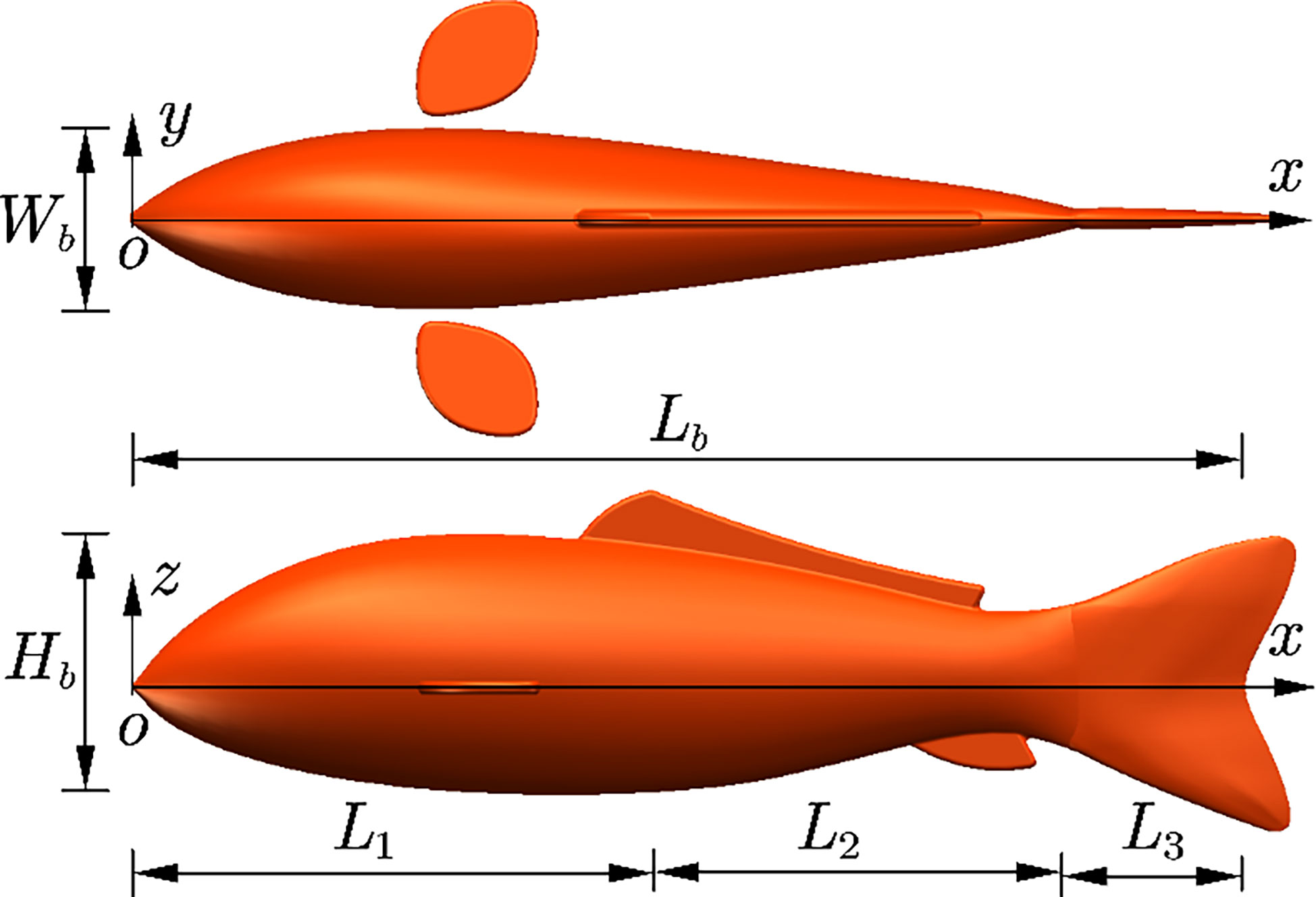
Figure 1 3D geometrical model of the fishlike swimmer. 3D, three-dimensional.

2.1.2 Morphological kinematic model

Fish has a flexible body and can swim with a variety of fluctuating motion principles, which is the key point of excellent swimming performance (Wang et al., 2022). As a result, when describing the fluctuating motion model of the fish body, flexibility must be taken into consideration. In the swimming process, the motion trajectory of the fish body’s midline can be precisely described by the traveling wave equation with a steadily rising amplitude (Cui et al., 2018).

The kinematic model specified by previous research (Xue et al., 2020) was adopted to describe the body’s deforming motion of the Carangiform swimmer to minimize the head yaw amplitude. The length of the entire body was used in dimensionless processing. Meanwhile, a time function (Curatolo and Teresi, 2016) was introduced to simulate the whole deformation process from a static state to a steady pace to deal with the starting divergence problem in the simulation. The optimized kinematic model of the swimmer’s midline can be expressed as follows:

$\begin{array}{ll}\begin{array}{c}y\left(x,t\right)=A{\left[\frac{s}{s-1}\frac{x}{L_b}-\frac{4}{5\left(s-1\right)}\right]}^{ϵ}\text{sin}\left(k\frac{x}{L_b}-2\pi ft\right)\left(1-e^{-\frac{t}{t_s}}\right)L_b\\ s\ge 3,ϵ\ge 1,0\le x\le L_b\end{array}& (1)\end{array}$

where x represents the displacement along the direction from the head to the tail, y represents the lateral undulation value of the midline in the body frame, t is the swimming time, f is the tail-beat frequency, k=2π/λ is the wave number, and λ is the wavelength. In addition, A and ε control the oscillating amplitude, and s describes the initial oscillating position at the body.

Assuming that the fishlike swimmer moves in a straight line along a set direction, without steering motion, and the fluctuation amplitude and period are constant. The body-caudal fin fluctuation of the fishlike swimmer can be regarded as periodic motion. The fluctuation curves of the midline in one tail-beat cycle are depicted in Figure 2, where λ=0.95 , A=0.1 , s=5 , and ϵ=3 .

FIGURE 2

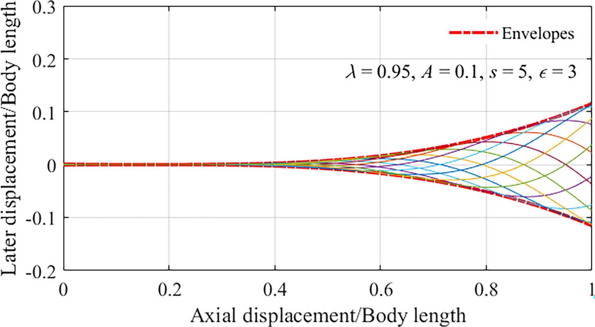
Figure 2 Midlines of the fish for different instants in one tail-beat cycle.

The hydrodynamic force generated by the pectoral fins of the swimmer is the key factor to achieve the motion in three dimensions. Although it is not the focus of this study, in order to simulate the swimming process more realistically, the effect of the pectoral fin on swimming was taken into consideration. The left and right pectoral fins were simply defined as simultaneous oscillations with equal angles. The oscillation equation of pectoral fins in the x–z plane can be defined as follows.

$\begin{array}{ll}\theta \left(t\right)={\theta }_{max}\text{sin}\left(2\pi ft+\phi \right)\left(1-e^{-\frac{t}{t_s}}\right)& (2)\end{array}$

where θ(t) represents the angular oscillation of the pectoral fins, θ_max is the maximum oscillation amplitude, and φ is the phase difference between the fluctuating motion of the body and oscillation of the fins.

2.2 Models of complex terrain

2.2.1 Undulating seabed boundary

When a robotic fish performs exploration and sampling near the seabed, the uneven seafloor surface constitutes the boundary of the motion space. The complex topography of the seafloor will significantly affect the flow field close to the seabed (Rogers et al., 2018) and further affect the swimming performance of the robotic fish. Compared to the size of the robotic fish, the scale of the terrain, such as a submarine mountain, cliff, and cave, is relatively large (Lecours et al., 2016). The effects on hydrodynamics caused by large-scale terrains change smoothly, which has little impact on the motion stability of the robotic fish. However, the structural characteristics, such as a small-scale undulation and a local bulge, have an obvious and sudden impact on the swimming performance, which should be taken into consideration.

The topography of the seafloor is intricately layered. In order to facilitate the quantitative description of the topography changes, the local undulation feature of the seabed was simplified using the stepped surface to describe the height change of the seabed. The height of the fish body H_b was used to nondimensionalize the distance H between the fish belly and the seafloor surface. The process of the robotic fish that swam near the stepped surface was simulated. As the robotic fish swam, the value of H decreased gradually, as shown in Figure 3. The impact of the seabed boundary modification on the swimming performance was examined. In this process, the values of H changed in the sequence as 5H_b, 2.5H_b, 1.25H_b, and 0.25H_b. Ahead of the comparison, the fishlike swimmer should reach to a steady speed to eliminate the influence of the starting process. Thus, the robotic fish swam a significant distance in the area where H was equal to 5H_b. In addition, the swimming distance was 3L_b at the condition where H was equal to 2.5H_b, 1.25H_b, or 0.25H_b.

FIGURE 3

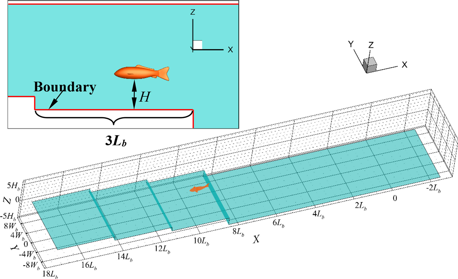
Figure 3 The undulating seabed boundary model.

2.2.2 The narrow channel

The fishlike propulsion mode has shown excellent mobility and flexibility, which makes fish or robotic fish swim in narrow channels easily. The flow field changes resulting from the two vertical boundary surfaces of narrow channels should be given enough attention when the robotic fish conducts underwater exploration and sampling (Ćatipović et al., 2019). Under the condition that the channel width is narrow, the impact of the boundary surfaces on the hydrodynamic characteristics of the swimmer is clear enough, which will affect the swimming performance. Especially during the processes of the swimmer entering the narrow channel from the open water and swimming from the narrow channel into the open water, the boundary conditions of the flow field change dramatically, which will disturb the motion state of the robotic fish. Then, the seabed exploration and sampling process will become unstable.

Similarly, the structure of the narrow channel was simplified. The two vertical boundary surfaces of the narrow-channel model were both set as plane, and the distance W from one side of the swimmer to the near narrow-channel boundary was nondimensionalized by the body width W_b, as shown in Figure 4. The continuous process of the swimmer moving into the narrow channel from the open water, passing the narrow channel, and subsequently moving out of the narrow channel to the open water was numerically simulated. The impact of the boundary on the motion stability of the swimmer was analyzed. In this process, the values of W changed in sequence as 10W_b, 5W_b, 1W_b, and 10W_b. Before moving into the narrow channel, the robotic fish swam a suitable distance in the area where W was equal to 10W_b before entering the narrow channel. The swimming distance was 3L_b at the condition where W was equal to 5W_b or 1W_b. The included angle between the transition connection surface and the boundary surface is 45 degrees.

FIGURE 4

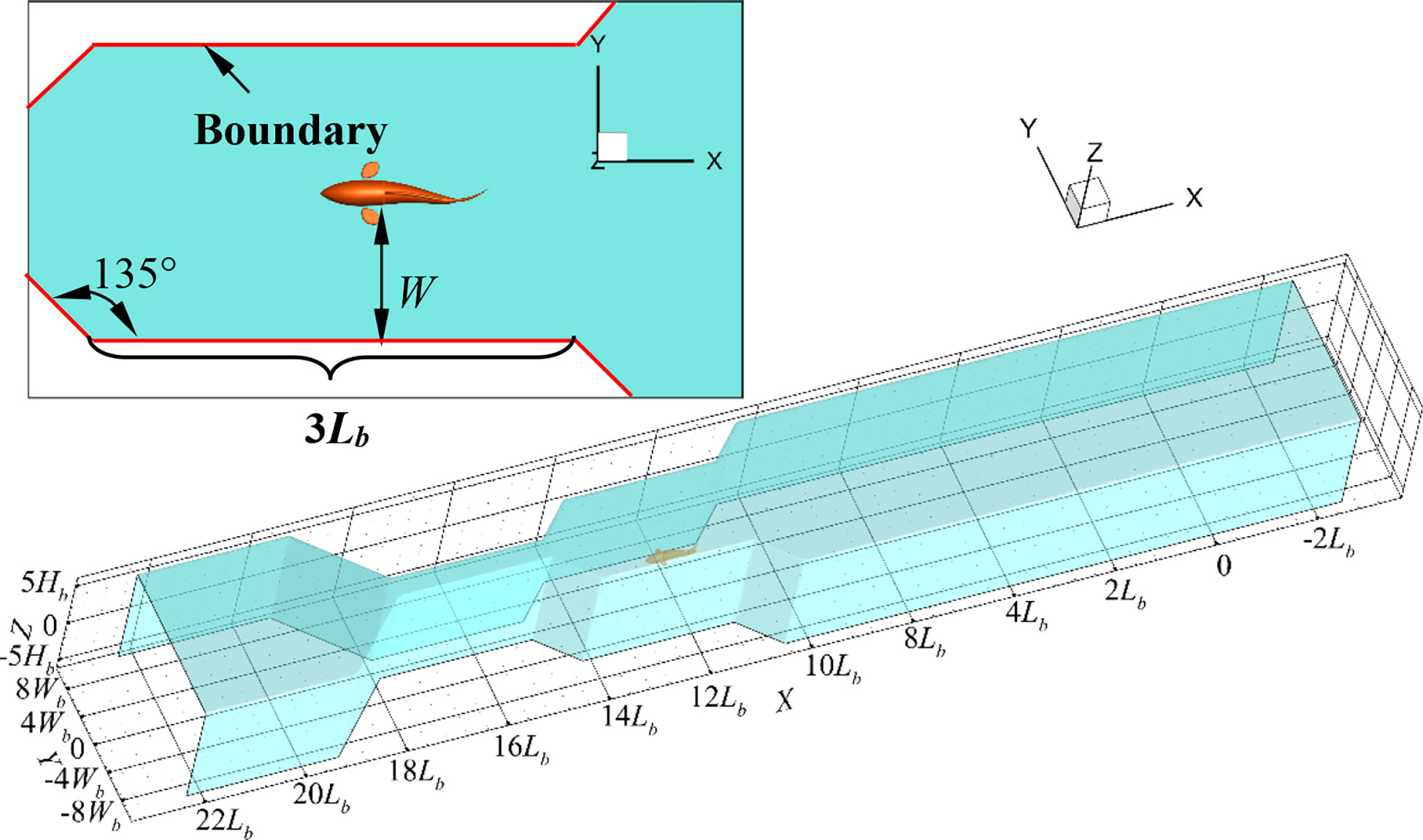
Figure 4 The narrow-channel boundary model.

3 Method

3.1 Computational methodology

3.1.1 Numerical implementation

According to the above definition of kinematics, the rolling and pitching DOFs of the swimmer can be ignored when swimming in 3D space. Thus, the fishlike swimmer can achieve three translational DOFs (forward translation x, lateral translation y, and vertical translation z) and one rotational DOF (yaw angle ψ) in the global frame OXYZ as shown in Figure 5. The generalized location X, velocity V, force F vectors, and the mass matrix M of the swimmer’s center of mass (COM) can be defined as follows:

FIGURE 5

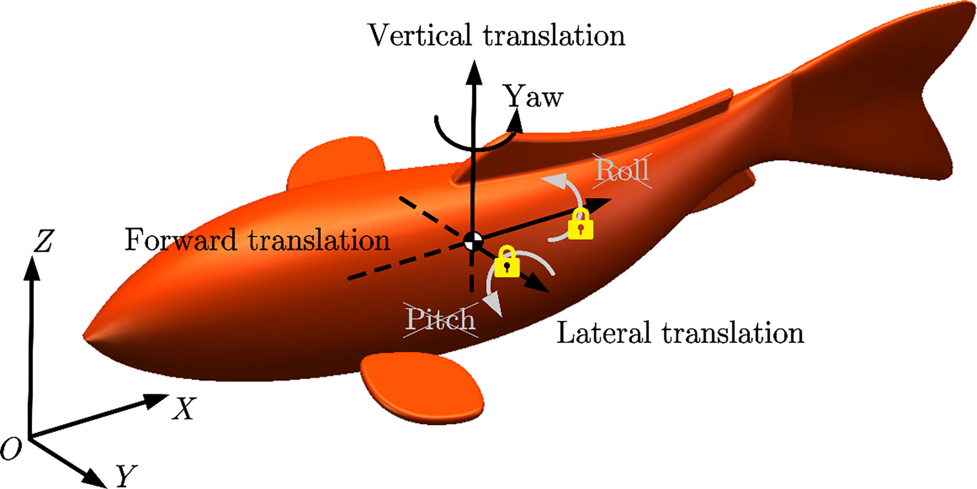
Figure 5 Sketch of the world frame OXYZ and the DOFs of the swimmer. DOFs, degree of freedoms.

$\begin{array}{ll}\mathit{X}=\left(\begin{array}{l}x\hfill \\ y\hfill \\ z\hfill \\ \psi \hfill \end{array}\right),\mathit{V}=\left(\begin{array}{c}u\\ v\\ w\\ r\end{array}\right),\mathit{F}=\left(\begin{array}{c}{F}_h^x\\ F_h^y\\ F_h^z\\ M_h^z\end{array}\right),\mathit{M}=\left(\begin{array}{cccc}m& 0& 0& 0\\ 0& m& 0& 0\\ 0& 0& m& 0\\ 0& 0& 0& I_z\end{array}\right)& (3)\end{array}$

where u, v, w, and r are the generalized velocity components corresponding to the generalized location, F_h is the force component in the corresponding directions, M_h is the moment component in the z-direction, m is the mass of the swimmer that has a density of ρ_b=ρ , and I_z is the moment of inertia to the COM. The 4-DOF motion of the self-propelled swimmer can be described as follows:

$\begin{array}{ll}\mathit{F}={\mathit{M}}_T\frac{d\mathit{V}}{dt}& (4)\end{array}$

where M_T is the generalized total mass matrix, M_T=M+M_A , and M_A is the generalized added mass matrix. The generalized instantaneous fluid force F can be calculated directly by the numerical simulation. The swimmer’s generalized location X and generalized velocity V of each time step Δt can be calculated from the force value and motion state at the previous time step in the numerical simulation.

The trapezoidal rule was used for numerical integration, such that the generalized variables at time (t+Δt) in the calculation process can be expressed as follows:

$\begin{array}{ll}\{\begin{array}{l}\mathit{V}\left(t+\text{Δ}t\right)=\mathit{V}\left(t\right)+{\mathit{M}}_T^{-1}\frac{\mathit{F}\left(t+\text{Δ}t\right)+\mathit{F}\left(t\right)}{2}\text{Δ}t\hfill \\ \mathit{X}\left(t+\text{Δ}t\right)=\mathit{X}\left(t\right)+\frac{\mathit{V}\left(t+\text{Δ}t\right)+\mathit{V}\left(t\right)}{2}\text{Δ}t\hfill \end{array}& (5)\end{array}$

3.1.2 Evaluation of the swimming performance

In this work, the variation of swimming efficiency and dimensionless hydrodynamic coefficients were used to evaluate the swimming performance of the fishlike swimmer under complex terrain changes.

Although there has been much discussion and controversy about the calculation method of the fishlike swimming efficiency (Schultz and Webb, 2002), the Froude efficiency was often adopted to quantify the swimming efficiency in most studies. Froude efficiency was a relatively reasonable parameter that indicated the proportion of the useful power to the total power, as follows (Borazjani and Sotiropoulos, 2008):

$\begin{array}{ll}\eta =\frac{\overline{T}{U}_s}{\overline{T}{U}_s+{\overline{P}}_y}& (6)\end{array}$

where $\overline{T}$is the average thrust, U_s is the steady swimming speed, and ${\overline{P}}_y$is the average power loss due to the lateral undulations. In order to obtain the Froude efficiency of the fishlike swimmer in the steady swimming process, the instantaneous thrust and lateral power should be clarified first.

In the numerical simulation, the fishlike swimmer swam along the x direction of the computational domain, from static state to steady motion until the thrust was approximately equal to the drag, which was a continuous process. The fluid force F along the x direction can be computed by integrating the pressure force and viscous force on the fish body (Borazjani and Sotiropoulos, 2008), as follows:

$\begin{array}{ll}F(t)={\int }_s(p{n}_x-{\tau }_{xj}{n}_j)dS& (7)\end{array}$

where p and τ are the pressure and viscous stress tensor, respectively, n_j is the j–th component of the unit normal vector on dS, n_x is the unit vector along the x direction, and S is the surface area of the swimmer’s body. To separate the contributions of thrust T(t) and drag D(t), the instantaneous net force F(t) can be decomposed as follows (Li et al., 2019):

$\begin{array}{ll}T(t)=0.5F(t)+0.5{\int }_s(\left|p{n}_x\right|+\left|{\tau }_{xj}{n}_j\right|)dS& (8)\end{array}$

$\begin{array}{ll}-D(t)=0.5F(t)-0.5{\int }_s(\left|p{n}_x\right|+\left|{\tau }_{xj}{n}_j\right|)dS& (9)\end{array}$

Moreover, the nondimensional thrust (C_T) and drag (C_D) coefficients along the x direction can be calculated as follows:

$\begin{array}{ll}{C}_T=\frac{T\left(t\right)}{0.5\rho U_s^2{L}_b^2}& (10)\end{array}$

$\begin{array}{ll}{C}_D=\frac{D\left(t\right)}{0.5\rho U_s^2{L}_b^2}& (11)\end{array}$

The swimming power loss due to lateral undulations of the body can be calculated as follows:

$\begin{array}{ll}{P}_y=\int {}_s(p{n}_y-{\tau }_{yj}{n}_j)u_{y}dS& (12)\end{array}$

where u_y is the lateral component of the body motion velocity.

The nondimensional lateral power loss coefficients can be defined as follows:

$\begin{array}{ll}{C}_P=\frac{P_y}{0.5\rho U_s^3{L}_b^2}& (13)\end{array}$

The effects of terrain change on the Froude efficiency and hydrodynamic coefficients were discussed in the following part.

3.1.3 Governing equations

The swimming process can be regarded as the research on the hydrodynamics and external flow field of a moving and undulating body in which the domain was occupied with an incompressible viscous fluid. The time-averaged continuity equation and the Reynolds-averaged Navier–Stokes (RANS) equations of incompressibility in the 3D Cartesian coordinate system can be used as the governing equations of the computational domain (Malalasekera and Versteeg, 2007), as follows:

$\begin{array}{ll}\{\begin{array}{c}\nabla ·U=0\\ \frac{\partial U}{\partial t}+\nabla ·\left(UU\right)+\nabla ·\left(\overline{u^{\prime }{u}^{\prime }}\right)=-\frac{1}{\rho }\frac{\partial P}{\partial x}+v{\nabla }^{2}U+f_1\\ \frac{\partial V}{\partial t}+\nabla ·\left(VU\right)+\nabla ·\left(\overline{v^{\prime }{u}^{\prime }}\right)=-\frac{1}{\rho }\frac{\partial P}{\partial y}+v{\nabla }^{2}V+f_2\\ \frac{\partial W}{\partial t}+\nabla ·\left(WU\right)+\nabla ·\left(\overline{w^{\prime }{u}^{\prime }}\right)=-\frac{1}{\rho }\frac{\partial P}{\partial z}+{\nabla }^{2}W+f_3\end{array}& (14)\end{array}$

where U is the average velocity vector (U, V, W), u^′ is the pulsation velocity vector (u^′, v^′, w^′) , P represents the average pressure, ρ is the density of the fluid, and f_i are the components of body force in different directions. The instantaneous velocity vector u(u, v, w)=U+u^′ .

3.2 Preparation and verification of the numerical simulation

In this study, the commercial software ANSYS Fluent was used for the numerical solution of the governing equations with fluid-motion interaction. The computational domain was discretized by meshes using the commercial software Fluent Meshing. In particular, the compiled user-defined function (UDF) programs were written to realize the deformation and self-propelled motion of the fishlike swimmer. The flow field was visualized by the commercial software Tecplot, and the data-processing work was realized by the commercial software MATLAB. The numerical simulation was carried out on the desktop workstation configured with 64-Core 128-Processor Intel(R) Xeon(R) Platinum 8375 CPU @2.80GHz and 256GB RAM. Additionally, it should be noted that the validation of the numerical simulation was carried out in the case where the robotic fish swam in a rectangular tank, rather than the above complex terrain model, to reduce the computing resources. In the simulation with the complex terrain model, the discretization method of the computational domain, the partition scale of the grid, and the calculation settings were the same as the validated process. When the difference of the mean swimming speed value between the two consecutive motion cycles was less than 5%, the motion state can be regarded as steady swimming.

3.2.1 Computational domain discretization and calculation setup

The computational domain of the verification work to simulate the self-propelled motion of the fishlike swimmer was a large enough cubic tank full of fresh water, whose size is 11L_b×20W_b×11H_b . The dynamic mesh technology based on the arbitrary Lagrangian–Eulerian (ALE) method was used in this study. However, it was difficult to deal with the complex self-propelled motion of the swimmer with body undulating and pectoral fins oscillating only using the dynamic mesh technology; the problem of negative volume mesh occurred frequently. Then, the overlapping grid technology was used to deal with that problem effectively (Li et al., 2012; Horne and Mahesh, 2019). Therefore, two sets of meshes were established: the poly-hexahedral global mesh was set as the background mesh and the triangular body-fixed mesh was set as the component mesh. The full tank was configured as the background mesh, and the swimmer was completely covered in the component mesh where the deformation of the swimmer was included. The dynamic mesh technology with diffusion smoothing method and remeshing method was used to deal with the large deformation of the component mesh, and the overset moving setup on the background mesh was used to define the relative motion between the swimmer and the global coordinate system.

The boundary conditions and meshes of the simulation domain are shown in Figure 6. Surface 1 was set to a velocity inlet with the velocity magnitude of 0 m/s to keep the water still, and surface 2 was set to a pressure outlet with the gauge pressure of 0 Pa. Surface 3 and surface 4 were no-slip walls, and the overset setup was imposed on surface 5.

FIGURE 6

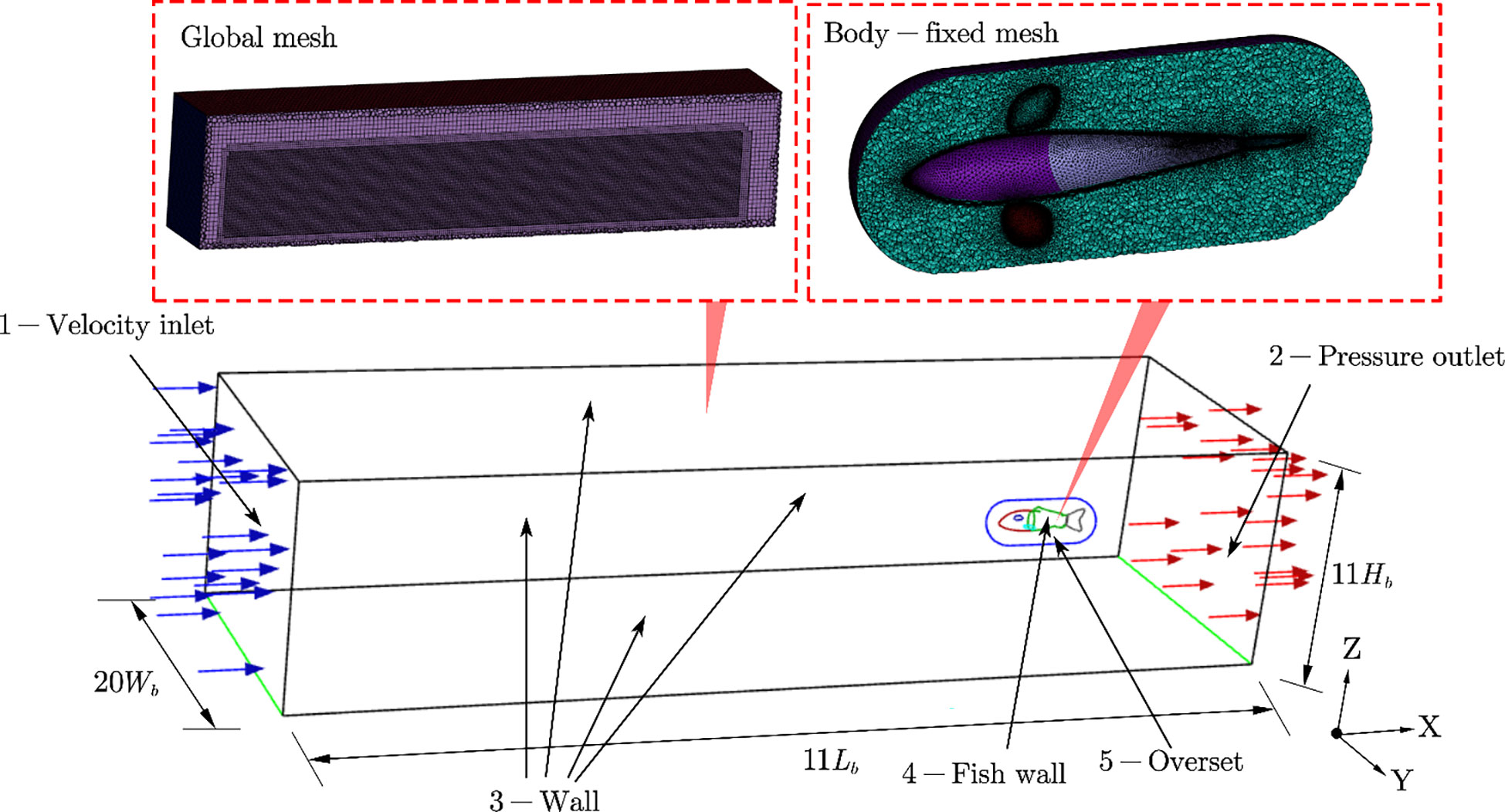
Figure 6 Meshes and boundary conditions.

The pressure-based solver, absolute velocity formulation, and transient time model were taken into utilization. The k−ω SST (shear stress transport) turbulence model with low Re adaptation was adopted to solve Eq. 14. The k−ω SST model was of relatively low computational cost and accurate calculation, which had good adaptability to the simulation of the boundary layer and free shear flow (Macias et al., 2020). In solution methods, the least-squares cell-based scheme was used for the gradient evaluation, the second-order discretization was used for the pressure term, and the second-order upwind scheme was used for the momentum term. Moreover, both the turbulent kinetic energy and turbulent dissipation rate were second-order upwind scheme; the transient formulation is first-order implicit type.

3.2.2 Independence validation and generalized added mass

In order to validate the independence of the mesh size to the simulation results, both the background mesh and component mesh of the computational domain were divided into five levels, as Coarse, Coarser, Normal, Finer, and Fine. Regardless of the mesh level, the local maximum size of the background mesh was four times its local minimum size, and the local maximum size of the component mesh was three times its local minimum size. The local minimum size of the five background meshes was 0.075 L_b, 0.0625 L_b, 0.05 L_b, 0.0375 L_b, and 0.025 L_b, and the local minimum size of the five component meshes was 0.015 L_b, 0.0125 L_b, 0.01 L_b, 0.0075 L_b, and 0.005 L_b. The minimum orthogonal quality of all meshes was required to be not less than 0.3. The tail-beat frequency f of 2.0Hz and other morphological kinematic parameters remained unchanged in the simulation with various meshes. The steady nondimensional forward velocity U_s/L_b was specified as the evaluation variable to verify the independence. Moreover, the maximum time step Δt_max was determined by the minimum mesh size and the maximum deforming velocity of the body. Similarly, five levels of the time step, T/80, T/100, T/200, T/400, and T/500, were divided to validate the independence of the time step, where T = 1/f. The validation results are shown in Figure 7.

FIGURE 7

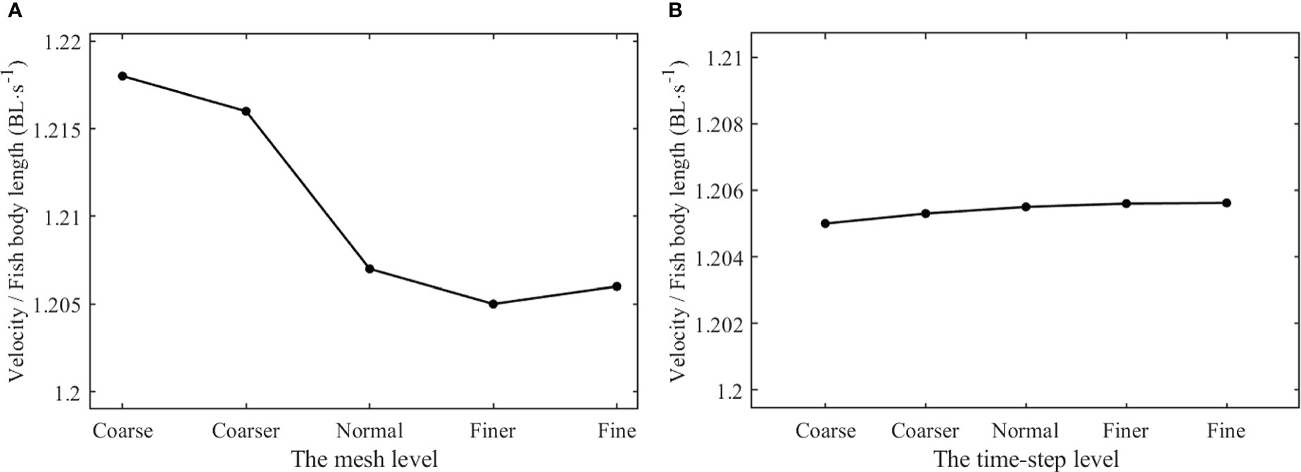
Figure 7 The values of nondimensional steady velocity for independence validation. (A) Independence validation of the mesh size (B) Independence validation of the time step.

It was clear that the forward velocity that remained almost unchanged are reaching Normal-level mesh according to Figure 7A. The excessive rough mesh would cause serious instability in simulation results when mesh deforming, and excessive fine mesh would lead to not only the waste of computing resources but also limitation in accuracy improvement. Thus, the Normal-level mesh was selected for the time-step independence validation and swimming process simulation. As shown in Figure 7B, the forward velocity did not respond significantly to the change of time-step level, and the time step T/100 was selected for the swimming process simulation.

In order to calculate the generalized added mass, the motions of the swimmer along various directions were defined as low-speed and small-amplitude sine oscillating movements of a rigid body.

$\begin{array}{ll}{v}_i=A_i\text{sin}{\omega }_{i}t& (15)\end{array}$

where the subscript i =1,2,3 represents the translational mode in three directions of Cartesian coordinate system, i=4 represents the rotational mode around the z direction, A_i is the amplitude of motion velocity, and ω_i is the motion frequency. In this paper, A_i=0.01 m/s and ω_i = 0.5 rad/s. The generalized hydrodynamic force of the swimmer was decomposed into the generalized viscous force and inertia force attributed to velocity and acceleration, respectively (Li et al., 2010). The overset mesh technology was also used to simulate these motions as Eq. 15, and the hydrodynamics F_h and M_h were recorded. The generalized force on the swimmer should be entirely supplied by the acceleration when the instantaneous speed was zero. Thus, the added mass can be obtained by dividing the hydrodynamic force in each direction by the corresponding acceleration with a zero instantaneous speed. The result of the generalized added mass matrix was calculated as follows:

$\begin{array}{ll}{\mathit{M}}_A=\left(\begin{array}{cccc}0.113m& 0& 0& 0\\ 0& 2.91m& 0& 0\\ 0& 0& 0.645m& 0\\ 0& 0& 0& 1.27I_z\end{array}\right)& (16)\end{array}$

The completed dynamic equation of the robotic fish system can be established by combining Eq. 4 with Eq. 16.

3.3 Swimming process simulation

In the numerical simulation, the swimming motions of the fishlike swimmer at three tail-beat frequencies (1.0Hz, 1.5Hz, 2.0Hz) in an undulating terrain and a narrow channel were simulated. In terms of the simulation domain, the maximum width was 20W_b and the maximum height was 11H_b, and in these circumstances, the fish body can be regarded to be free swimming without effect of the up-down and left-right boundary based on the validation results. When the robotic fish swam forward gradually along the x direction, the changing topography would gradually affect the hydrodynamic characteristics and swimming performance of the swimmer.

4 Results and discussion

4.1 Effects of complex terrain on the swimming performance

4.1.1 Forward speed

The forward swimming speeds of the fishlike swimmer are depicted in Figures 8A and 9A with changes in the tail-beat frequency f, the dimensionless height H, and the dimensionless distance W. The unit BL·s⁻¹ used to describe the forward speed means the body length per second. The swimmer with different tail-beat frequencies swam across various terrain conditions, but the changing pattern of the forward speed was consistent. From the starting static state to a steady swimming condition, the forward speed gradually rose until reaching an asymptotic stable value. The forward speed rose as the tail-beat frequency rose, and the instantaneous speed fluctuated periodically, matching the tail-beat period.

FIGURE 8

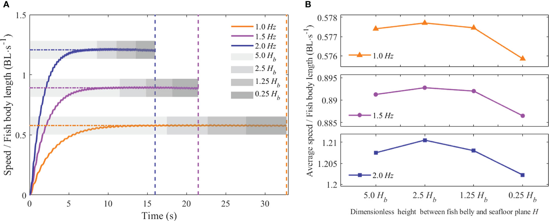
Figure 8 Forward speed of the swimmer at different values of f and H (A) Instantaneous forward speed (B) Average forward speed.

FIGURE 9

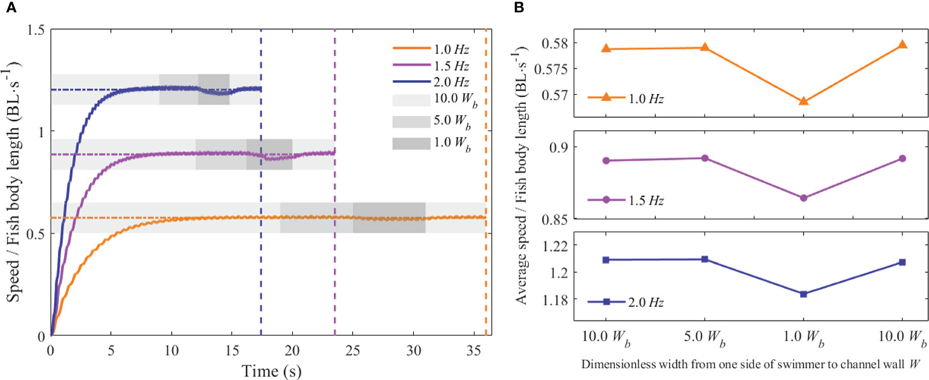
Figure 9 Forward speed of the swimmer at different values of f and W. (A) Instantaneous forward speed (B) Average forward speed.

Furthermore, the average forward speeds at different tail-beat frequencies, dimensionless height H, and dimensionless distance W were calculated. The effects of the above dimensionless distance parameters on the average forward velocity are described in Figures 8B and 9B. As shown in Figure 8B, when the dimensionless distance H was larger than 1.25H_b, the average forward speed varied little at different tail-beat frequencies. When the value of H was 0.25H_b, the average forward speed had a relatively small reduction approximately 0.3%–0.8% compared with that of the value of 1.25 H_b at different tail-beat frequencies. Figure 9B demonstrated that when the dimensionless distance W was larger than 5W_b, the average forward velocity had almost no change under different tail-beat frequencies. When the value of W reached 1W_b, corresponding to the three tail-beating frequencies of 1, 1.5, and 2.0 Hz, the average forward speed decreased by 1.82%, 2.41%, and 3.11%, respectively, compared with that of the value of 5W_b. When the value of W got back to 10W_b, the average forward speed increased synchronously. As a result, it was believed that the swimming boundary’s bottom had little influence on the swimmer’s swimming speed, but the forward speed would be slowed when the swimmer passed through the narrow channel. The higher the tail-beat frequency, the larger the decline.

4.1.2 Froude efficiency and hydrodynamic coefficients

A previous study (Takahashi et al., 2020) has shown that the Carangiform kinematic mode of self-propelled constant-speed swimming was inefficient at low Re. The model specified in this work guaranteed that the swimmer maintained a high Re at all tail-beat frequencies, exceeding 10,000. Figure 10 shows the change of Froude efficiency with dimensionless distance under various swing frequencies. Although there is a considerable variation in Froude efficiency under various swing frequencies, the distance parameter did not appear to have a major impact on it. The efficiency was maintained at a nearly constant value for each motion mode. It was worth mentioning that Froude efficiency appeared to increase with frequency. In order to further verify this point, the Strouhal number (St) based on tail-beat frequency f, tail-beat amplitude A, and steady forward speed U_s was calculated according to Eq. 17, and it characterized the swimmer’s undulation performance. The values are 0.176, 0.171, and 0.165, respectively, under tail-beat frequencies of 1.0, 1.5, and 2.0 Hz. The results discovered that St gradually decreased as frequency increased. In fact, the swimmer at higher St indicated quicker lateral undulations, resulting in a higher lateral power loss and lesser efficiency, and which was consistent with the findings of this work.

FIGURE 10

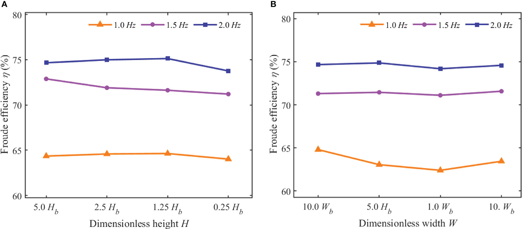
Figure 10 Froude efficiency of the swimmer at different values of f, H, and W. (A) Froude efficiency at different values of f and H (B) Froude efficiency at different values of f and W.

$\begin{array}{ll}St=\frac{fA}{U_s}& (17)\end{array}$

Several typical cycles in 2 s of instantaneous hydrodynamic coefficients, at different tail-beat frequencies for H=5.0H_b and W=10.0W_b , are presented in Figure 11. Throughout the whole swimming process, the swimmer needed various time lengths with different tail-beat frequencies because a lower tail-beat frequency motion took a longer time to reach a stable speed. Thus, the “a” in the horizontal axis of Figure 11 denoted the specific starting time after the swimmer reached a constant swimming speed at each tail-beat frequency. As can be observed in Figure 11, at each frequency, the thrust coefficient and drag coefficient changed on a regular basis, with the average values being about the same during an entire cycle. It indicated that the thrust forces and drag forces acting on the swimmer were almost the same, and the swimmer reached a stable swimming state. The fluctuation of the thrust coefficient was negligible compared to the drag coefficient. Moreover, the lateral fluctuation power that fluctuated around zero was likewise consistent with the expected value, since the swimmer merely swam in a straight line.

FIGURE 11

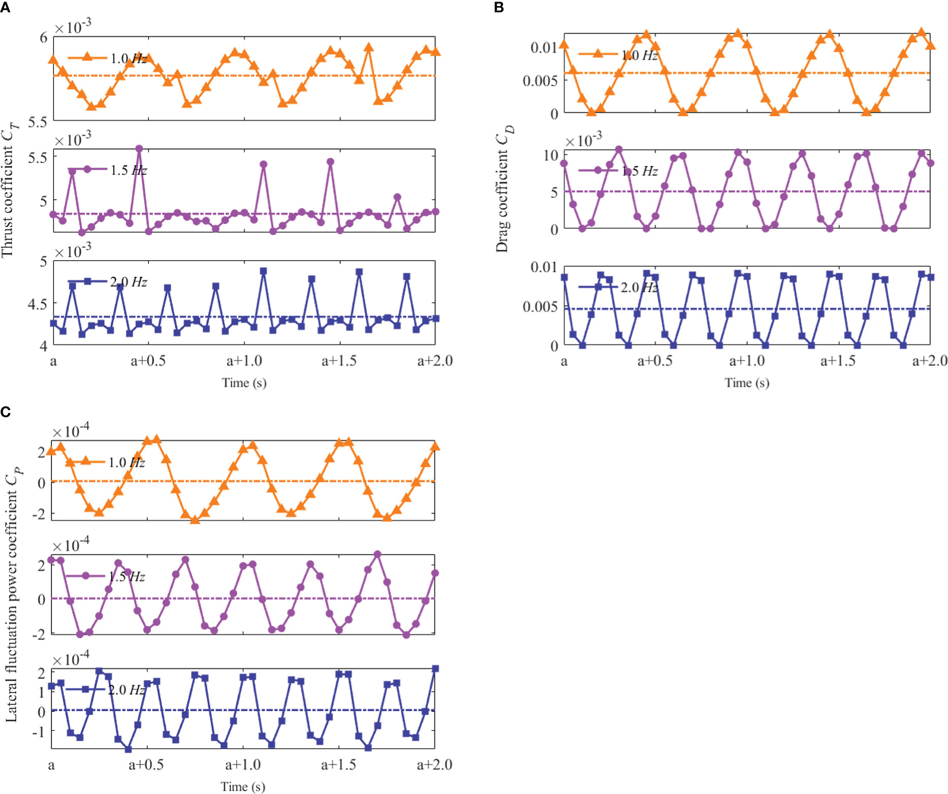
Figure 11 Hydrodynamic coefficients of the swimmer at different tail-beat frequencies f (A) Thrust coefficient C_T (B) Drag coefficient C_D (C) Lateral fluctuation power coefficient C_p.

The influence of the dimensionless distance parameter on the periodic stability of the hydrodynamic coefficient was another point of concern. The standard deviation of the hydrodynamic coefficient across successive time periods was used to assess that impact. Figures 12A, B show the effect of the changed H and W on the thrust coefficient, drag coefficient, and lateral fluctuation power coefficient at different tail-beat frequencies. The standard deviations of the three hydrodynamic coefficients had similar overall fluctuation patterns. As illustrated in Figure 12A, when H was more than 1.25H_b, the standard deviation remained rather steady. However, when H hit 0.25H_b, the standard deviation increased. As illustrated in Figure 12B, the standard deviation of the three hydrodynamic coefficients tended to grow when the value of W decreased. When the value of W was reduced to 1.0W_b, the standard deviation increased, then dropped when the value of W returned to 10.0W_b. It indicated that although terrain changes had a limited impact on swimmers’ hydrodynamic coefficients, the surface had a large disturbance effect on swimmers’ hydrodynamic coefficients and force when approaching the bottom of the swimming boundary or passing through a narrow channel.

FIGURE 12

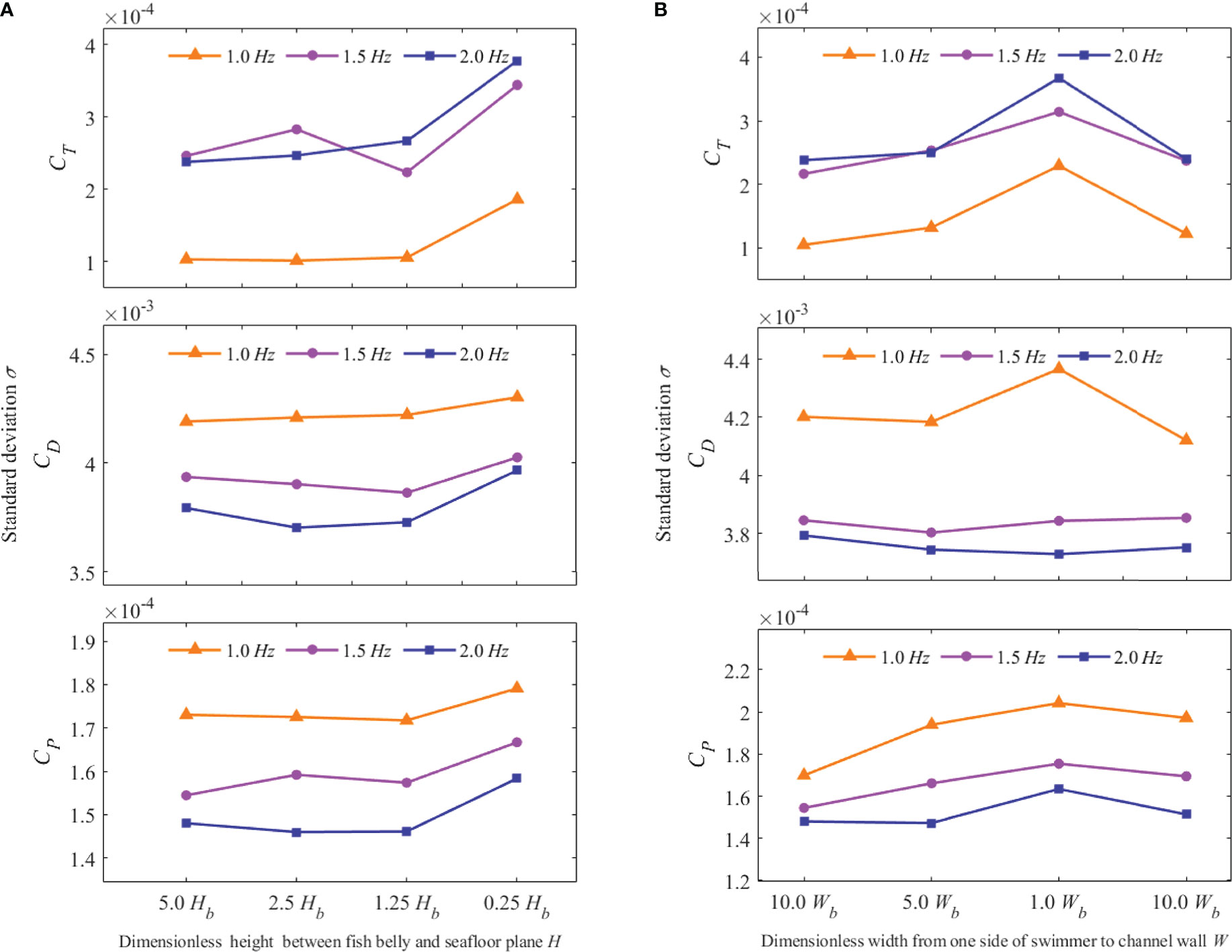
Figure 12 Hydrodynamic coefficient standard deviation of the swimmer at different values of f, H, and W. (A) Hydrodynamic coefficient standard deviation at different values of f and H (B) Hydrodynamic coefficient standard deviation at different values of f and W.

4.2 Evolution of the pressure field

In order to explore the influence mechanism of the complex terrain to Froude efficiency and hydrodynamic coefficients of the fishlike swimmer, the pressure field of the research domain was visualized by the pressure isosurface, as shown in Figure 13. The light color surface represents the relative pressure value 10 Pa, and the dark color surface represents the relative pressure value -10 Pa.

FIGURE 13

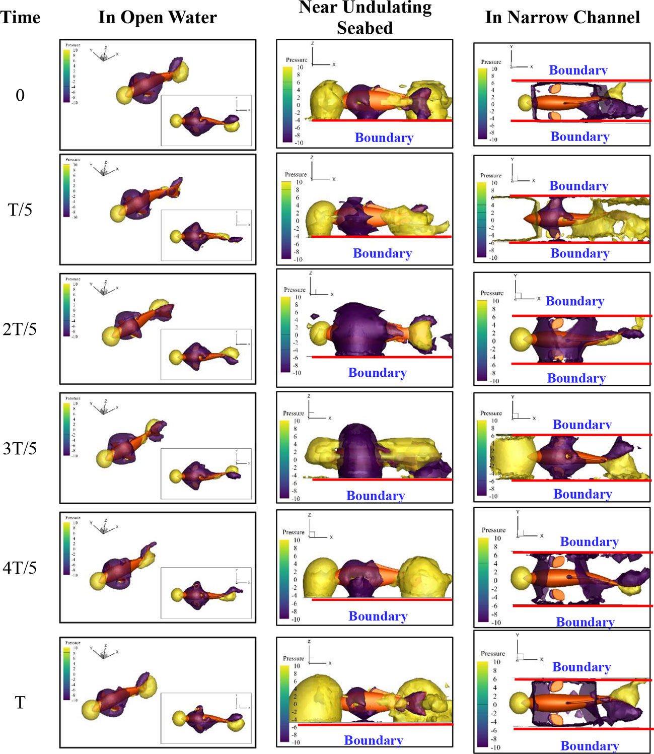
Figure 13 Pressure field of the research domain.

In Figure 13, there was a high-pressure area near the head part of the fishlike swimmer and a low-pressure area at the middle part. These two pressure areas would generate drag force on the swimmer. Moreover, at the tail part, the high-pressure area and low-pressure area appeared in pairs, which would generate thrust force and lateral force.

In the open water, the evolution of the pressure isosurface was stable, and the swimming mode was the only factor to affect the Froude efficiency and hydrodynamic coefficients. When a boundary surface appeared near the bottom of the swimmer, a part of the pressure area was blocked out by the boundary surface, and the force generated by the pressure difference would decrease. Then, the swimming process would be less efficient and the hydrodynamic coefficients would become smaller. Moreover, when the boundary surface appeared on both sides of the swimmer, more pressure areas would be blocked out, and the propulsion efficiency would be further reduced. That was the reason that the average forward speed had a small reduction under the undulating seabed boundary condition and a relatively large reduction under the narrow-channel boundary condition, as shown in Figures 8 and 9. Furthermore, two boundary surfaces at both sides of the swimmer would make the evolution of pressure field more complex, the standard deviation of hydrodynamic coefficients would increase, and the swimming stability would decrease, which was consistent with the results in Figure 12.

Thus, if the distance between the fish belly and the seafloor surface was large, perhaps larger than 0.25H_b, there was no need to worry about the impact on forward speed. But the swimmer should improve tail-beat frequency to keep a steady speed when passing through a narrow channel, especially for the condition where the distance from one side of the swimmer to the near boundary was smaller than 1W_b.

4.3 Evolution of the vortex distribution

On the other hand, the wake vortex contains the secret of highly efficient swimming of the fishlike swimmer (Harvey et al., 2022). The isosurface of Q-criterion has been used extensively as standard recognition of vortex (Ren et al., 2022). The evolution of the vortex distribution around the swimmer was visualized by the Q-criterion isosurface whose value was equal to 0.1, as shown in Figure 14.

FIGURE 14

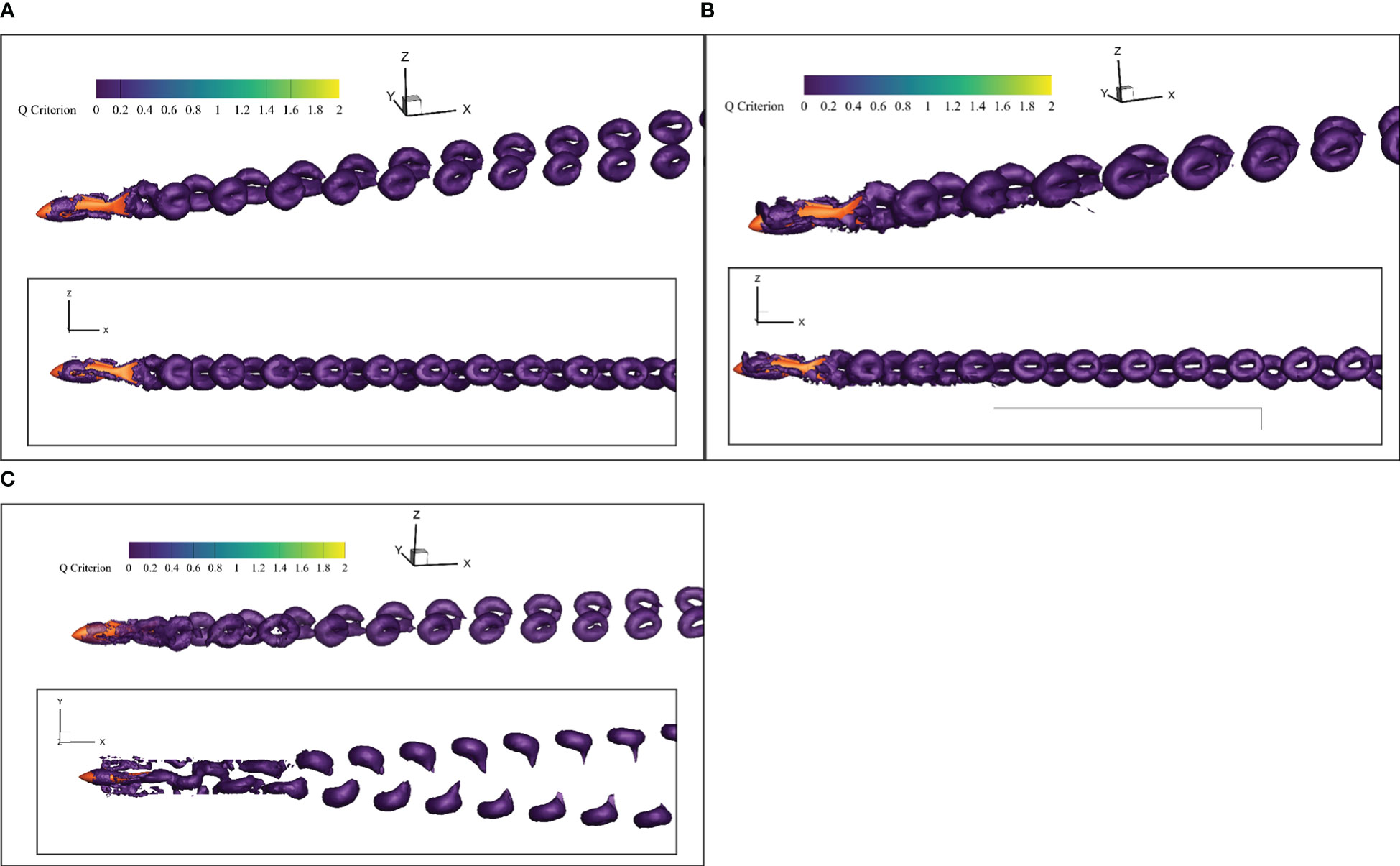
Figure 14 Vortex distribution of the research domain. (A) In Open Water (B) Near Undulating Seabed (C) In Narrow Channel.

In Figure 14, the vortex rings appeared in pairs after the swimmer to form the reverse Kaman vortex street. Then, the reverse Kaman vortex street would induce a jet effect to generate a positive force and the force was applied to the swimmer to make the swimmer get high Froude efficiency. Thus, the fishlike swimming mode had a higher propulsion efficiency than the propeller-driven mode.

In the open water, the wake vortex evolved freely and gradually dissipated under the viscosity effect of the water. The positive force induced by the reverse Kaman vortex street was large, and the additional efficiency was high. Meanwhile, in the evolution process, the vortex ring diffused to the rear on both sides of the robotic fish, not above or below the swimmer. The height of the vortex ring near the tail was almost equal to that of the fish body. Thus, under the undulating seabed condition, the boundary surface near the bottom of the swimmer had little effect on the swimming efficiency. However, when the boundary surfaces were at both sides of the swimmer, like the narrow-channel condition, the wake vortex would hit the boundary surface and dissipate rapidly. Almost no jet effect was induced, and the additional efficiency was small. That was the reason that Froude efficiency had little reduction under the undulating seabed boundary condition and a relatively large reduction under the narrow-channel boundary condition, especially when the tail-beat frequency was 1.0 Hz, as shown in Figure 10.

When the robotic fish swam near the undulating seabed, the evolution of the vortex distribution would not be seriously affected, and it was recommended to keep the tail-beat frequency unchanged. But when the robotic fish passed through the narrow channel, a large tail-beat frequency was needed to get enough thrust force.

5 Conclusion

In this paper, the swimming processes of robotic fish under an undulating seabed condition and a narrow-channel condition were studied. The forward speed, Froude efficiency, and hydrodynamic coefficients were calculated to evaluate the influence of complex terrain on the swimming performance. Moreover, the evolution processes of the pressure field and vortex distribution were visualized to discuss the influence mechanism. The key points of this paper can be summarized as follows:

1) The influence of the undulating seabed condition on the swimming performance of robotic fish was small, but the change in the swimming stability should be given sufficient attention when robotic fish swam near the undulating seabed with the distance about 0.25H_b.

2) The influence of the narrow-channel condition on the swimming performance was obvious because the boundary surface at both sides of the swimmer restricted the pressure field evolution and the vortex distribution evolution seriously. When robotic fish swam through a narrow channel at a certain tail-beat frequency, the forward speed and Froude efficiency decreased, and the swimming stability got worse.

3) In order to keep a good motion performance of the fishlike swimming mode when passing through a narrow channel, it was recommended to improve the tail-beat frequency. However, considering the swimming stability, the tail-beat frequency was not the larger the better.

In the future, the development of a physical robotic fish is expected. Various sensors should be integrated to record the force and motion state when the robotic fish conducts exploring and sampling in the deep sea. Experimental data will be helpful for further research on swimming performance optimization of the robotic fish and for the development of a low-disturbance bionic exploring and sampling platform.

Data availability statement

The raw data supporting the conclusions of this article will be made available by the authors, without undue reservation.

Author contributions

Conceptualization, GX; methodology, GX and FB; software and algorithm, FB; validation and analysis, GX and FB; visualization, FB and PR; investigation, PR; data curation, PR; writing-original draft preparation, GX and FB; writing-review and editing, GX and FB; supervision, YL; project administration, LG and YL; funding acquisition, LG and YL. All authors contributed to the article and approved the submitted version.

Funding

The research was supported by the National Natural Science Foundation of China (NO.52001186), the Natural Science Foundation of Shandong Province (NO.ZR2020QE292), the Open Fund Project of Key Laboratory of Ocean Observation Technology (NO. 2021klootA01), and the Science and Technology Innovation Project of Laoshan Laboratory (NO.LSKJ202203505), hereby thanks.

Conflict of interest

The authors declare that the research was conducted in the absence of any commercial or financial relationships that could be construed as a potential conflict of interest.

Publisher’s note

All claims expressed in this article are solely those of the authors and do not necessarily represent those of their affiliated organizations, or those of the publisher, the editors and the reviewers. Any product that may be evaluated in this article, or claim that may be made by its manufacturer, is not guaranteed or endorsed by the publisher.

References

Ćatipović I., Ušćumlić J., Ćustić L. (2019). Optimization of a subsea pipeline route profile with the elimination of free spans. J. Pipeline Syst. Eng. Pract. 10 (2), 04019007. doi: 10.1061/(ASCE)PS.1949-1204.0000375

CrossRef Full Text | Google Scholar

Borazjani I., Sotiropoulos F. (2008). Numerical investigation of the hydrodynamics of carangiform swimming in the transitional and inertial flow regimes. J. Exp. Biol. 211 (10), 1541–1558. doi: 10.1242/jeb.015644

PubMed Abstract | CrossRef Full Text | Google Scholar

Cui Z., Yang Z., Shen L., Jiang H. Z. (2018). Complex modal analysis of the movements of swimming fish propelled by body and/or caudal fin. Wave motion 78, 83–97. doi: 10.1016/j.wavemoti.2018.01.001

CrossRef Full Text | Google Scholar

Curatolo M., Teresi L. (2016). Modeling and simulation of fish swimming with active muscles. J. Theor. Biol. 409, 18–26. doi: 10.1016/j.jtbi.2016.08.025

PubMed Abstract | CrossRef Full Text | Google Scholar

Dhongdi S. C. (2022). Review of underwater mobile sensor network for ocean phenomena monitoring. J. Network Comput. Appl. 103418. doi: 10.1016/j.jnca.2022.103418

CrossRef Full Text | Google Scholar

Dong C., Zhu Z., Li Z., Shi X., Cheng S. J., Fan P. (2022). Design of fishtail structure based on oscillating mechanisms using PVC gel actuators. Sensors Actuators A: Phys. 341, 113588. doi: 10.1016/j.sna.2022.113588

CrossRef Full Text | Google Scholar

Feng H., Yu J., Huang Y., Qiao J. A., Wang Z. Y., Xie Z. B., et al. (2021). Adaptive coverage sampling of thermocline with an autonomous underwater vehicle. Ocean Eng. 233, 109151. doi: 10.1016/j.oceaneng.2021.109151

CrossRef Full Text | Google Scholar

Fossum T. O., Norgren P., Fer I., Nilsen F., Koenig Z. C., Ludvigsen M. (2021). Adaptive sampling of surface fronts in the Arctic using an autonomous underwater vehicle. IEEE J. Oceanic Eng. 46 (4), 1155–1164. doi: 10.1109/JOE.2021.3070912

CrossRef Full Text | Google Scholar

Ghommem M., Bourantas G., Wittek A., Miller K., Hajj M. R. (2020). Hydrodynamic modeling and performance analysis of bio-inspired swimming. Ocean Eng. 197, 106897. doi: 10.1016/j.oceaneng.2019.106897

CrossRef Full Text | Google Scholar

Hang H., Heydari S., Costello J. H., Kanso E. (2022). Active tail flexion in concert with passive hydrodynamic forces improves swimming speed and efficiency. J. Fluid Mechanics 932. doi: 10.1017/jfm.2021.984

CrossRef Full Text | Google Scholar

Harvey S. T., Muhawenimana V., Müller S., Wilson C. A. M. E., Denissenko P. (2022). An inertial mechanism behind dynamic station holding by fish swinging in a vortex street. Sci. Rep. 12 (1), 1–9. doi: 10.1038/s41598-022-16181-8

PubMed Abstract | CrossRef Full Text | Google Scholar

He S., Peng Y., Jin Y., Wan B. Y., Liu G. P. (2020). Review and analysis of key techniques in marine sediment sampling. Chin. J. Mechanical Eng. 33 (1), 1–17. doi: 10.1186/s10033-020-00480-0

CrossRef Full Text | Google Scholar

Hoar W. S., Randall D. J., Donaldson E. M. (1983). Fish physiology (Academic Press).

Google Scholar

Horne W. J., Mahesh K. (2019). A massively-parallel, unstructured overset method to simulate moving bodies in turbulent flows. J. Comput. Phys. 397, 108790. doi: 10.1016/j.jcp.2019.06.066

CrossRef Full Text | Google Scholar

Jiang Z., Lu B., Wang B. A., Cui W. C., Zhang J. F., Luo R. L., et al. (2022). A prototype design and Sea trials of an 11,000 m autonomous and remotely-operated vehicle dream chaser. J. Mar. Sci. Eng. 10 (6), 812. doi: 10.3390/jmse10060812

CrossRef Full Text | Google Scholar

Lecours V., Dolan M. F. J., Micallef A., Lucieer V. L. (2016). A review of marine geomorphometry, the quantitative study of the seafloor. Hydrology Earth System Sci. 20 (8), 3207–3244. doi: 10.5194/hess-20-3207-2016

CrossRef Full Text | Google Scholar

Li G., Chen X., Zhou F., et al. (2021). Self-powered soft robot in the Mariana trench. Nature 591 (7848), 66–71. doi: 10.1038/s41586-020-03153-z

PubMed Abstract | CrossRef Full Text | Google Scholar

Li X., Gu J., Su Z., Su Z., Yao Z. Q. (2021). Hydrodynamic analysis of fish schools arranged in the vertical plane. Phys. Fluids 33 (12), 121905. doi: 10.1063/5.0073728

CrossRef Full Text | Google Scholar

Li S. M., Li C., Xu L. Y., Yang W. J., Chen X. C. (2019). Numerical simulation and analysis of fish-like robots swarm[J]. Appl. Sci. 9 (8), 1652. doi: 10.3390/app9081652

CrossRef Full Text | Google Scholar

Li J., Lu C., Huang X. (2010). Calculation of added mass of a vehicle running with cavity. J. Hydrodynamics 22 (3), 312–318. doi: 10.1016/S1001-6058(09)60060-3

CrossRef Full Text | Google Scholar

Li G., Müller U. K., van Leeuwen J. L., Liu H. (2012). Body dynamics and hydrodynamics of swimming fish larvae: A computational study. J. Exp. Biol. 215 (22), 4015–4033. doi: 10.1242/jeb.071837

PubMed Abstract | CrossRef Full Text | Google Scholar

Macias M. M., Souza I. F., Brasil A. C. P., Oliveira T. F. (2020). Three-dimensional viscous wake flow in fish swimming-a CFD study. Mechanics Res. Commun. 107, 103547. doi: 10.1016/j.mechrescom.2020.103547

CrossRef Full Text | Google Scholar

Malalasekera W., Versteeg H. K. (2007). An introduction to computational fluid dynamics :the finite volume method. 2nd ed. ed Vol. 503 (Harlow, England: Pearson Education Ltd).

Google Scholar

Ma H. W., Ren S., Wang J. X., Ren H., Liu Y., Bi S. S. (2021). Research on the influence of ground effect on the performance of robotic fish propelled by oscillating paired pectoral fins. Ind. Robot: Int. J. robotics Res. Appl. 48 (1), 133–141. doi: 10.1108/IR-04-2020-0081

CrossRef Full Text | Google Scholar

Ogata Y., Azama T., Moriyama Y. (2017). Numerical investigation of small fish accelerating impulsively to terminal speed. J. Fluid Sci. Technol. 12 (1), JFST0009–JFST0009. doi: 10.1299/jfst.2017jfst0009

CrossRef Full Text | Google Scholar

Quinn D. B., Lauder G. V., Smits A. J. (2014). Flexible propulsors in ground effect. Bioinspiration biomimetics 9 (3), 036008. doi: 10.1088/1748-3182/9/3/036008

PubMed Abstract | CrossRef Full Text | Google Scholar

Ren X. T., Guo Y. L., Shen S. Q., Zhang K. (2022). Large Eddy simulation of flow field in thermal vapor compressor. Front. Energy Res. 10, 1008927. doi: 10.3389/fenrg.2022.1008927

CrossRef Full Text | Google Scholar

Rogers J. S., Maticka S. A., Chirayath V., Woodson C. B., Alonso J. J., Monismith S. G. (2018). Connecting flow over complex terrain to hydrodynamic roughness on a coral reef. J. Phys. Oceanography 48 (7), 1567–1587. doi: 10.1175/JPO-D-18-0013.1

CrossRef Full Text | Google Scholar

Schultz W. W., Webb P. W. (2002). Power requirements of swimming: Do new methods resolve old questions? Integr. Comp. Biol. 42 (5), 1018–1025. doi: 10.1093/icb/42.5.1018

PubMed Abstract | CrossRef Full Text | Google Scholar

Takahashi T., Yoshino S., Takaya Y., Nozaki T., Ohki K., Ohki T., et al. (2020). Quantitative in situ mapping of elements in deep-sea hydrothermal vents using laser-induced breakdown spectroscopy and multivariate analysis. Deep Sea Res. Part I: Oceanographic Res. Papers 158, 103232. doi: 10.1016/j.dsr.2020.103232

CrossRef Full Text | Google Scholar

Wang C. C., Lu J., Ding X. L., Jiang C. X., Yang J. Y., Shen J. H. (2021). Design, modeling, control, and experiments for a fish-robot-based IoT platform to enable smart ocean. IEEE Internet Things J. 8 (11), 9317–9329. doi: 10.1109/JIOT.2021.3055953

CrossRef Full Text | Google Scholar

Wang Z., Wang L. Y., Wang T., Zhang B. (2022). Research and experiments on electromagnetic-driven multi-joint bionic fish. Robotica 40 (3), 720–746. doi: 10.1017/S0263574721000771

CrossRef Full Text | Google Scholar

Wang R., Wang S., Wang Y., Cheng L., Tan M. (2022). Development and motion control of biomimetic underwater robots: A survey. IEEE Trans. Systems Man Cybernetics: Syst. 52 (2), 833–844. doi: 10.1109/TSMC.2020.3004862

CrossRef Full Text | Google Scholar

Wei Z. F., Li W. L., Li J., Chen J., Xin Y. Z., He L. S., et al. (2020). Multiple in situ nucleic acid collections (MISNAC) from deep-sea waters. Front. Mar. Sci. 7, 81. doi: 10.3389/fmars.2020.00081

CrossRef Full Text | Google Scholar

Whitt C., Pearlman J., Polagye B., Caimi F., Muller-Karger F., Copping A., et al. (2020). Future vision for autonomous ocean observations. Front. Mar. Sci. 697. doi: 10.3389/fmars.2020.00697

CrossRef Full Text | Google Scholar

Windsor S. P., Norris S. E., Cameron S. M., Mallinson G. D., Montgomery J. C. (2010). The flow fields involved in hydrodynamic imaging by blind Mexican cave fish (Astyanax fasciatus). part II: Gliding parallel to a wall. J. Exp. Biol. 213 (22), 3832–3842. doi: 10.1242/jeb.040790

PubMed Abstract | CrossRef Full Text | Google Scholar

Xie O., Yao J., Fan X. Z., Shen C., Zhang C. B. (2022). Numerical and experimental study on the hydrodynamics of a three-dimensional flapping caudal fin in ground effect. Ocean Eng. 260, 112049. doi: 10.1016/j.oceaneng.2022.112049

CrossRef Full Text | Google Scholar

Xing C., Cao Y., Cao Y. H., Pan G., Huang Q. G. (2022). Asymmetrical oscillating morphology hydrodynamic performance of a novel bionic pectoral fin. J. Mar. Sci. Eng. 10 (2), 289. doi: 10.3390/jmse10020289

CrossRef Full Text | Google Scholar

Xu Y., Mohseni K. (2016). A pressure sensory system inspired by the fish lateral line: Hydrodynamic force estimation and wall detection. IEEE J. Oceanic Eng. 42 (3), 532–543. doi: 10.1109/JOE.2016.2613440

CrossRef Full Text | Google Scholar

Xue G., Yanjun L., Weiwei S., Yifan X., Fengxiang G., Zhitong L. (2020). Evolvement rule and hydrodynamic effect of fluid field around fish-like model from starting to cruising. Eng. Appl. Comput. Fluid Mechanics 14 (1), 580–592. doi: 10.1080/19942060.2020.1734095

CrossRef Full Text | Google Scholar

Yoerger D. R., Govindarajan A. F., Howland J. C., Llopiz J. K., Wiebe P. H., Curran M., et al. (2021). A hybrid underwater robot for multidisciplinary investigation of the ocean twilight zone. Sci. Robotics 6 (55), eabe1901. doi: 10.1126/scirobotics.abe1901

CrossRef Full Text | Google Scholar

Zhang J. X., Liu M. Q., Zhang S. L., Zheng R. H., Dong S. L. (2022). Multi-AUV adaptive path planning and cooperative sampling for ocean scalar field estimation. IEEE Trans. Instrumentation Measurement 71, 1–14. doi: 10.1109/TIM.2022.3167784

CrossRef Full Text | Google Scholar

Zhong Y., Li Z., Du R. (2018). Robot fish with two-DOF pectoral fins and a wire-driven caudal fin. Advanced robotics 32 (1), 25–36. doi: 10.1080/01691864.2017.1392344

CrossRef Full Text | Google Scholar