Scale dependence of near-inertial wave’s concentration in anticyclones

Near-inertial waves (NIWs), pervasive and dominating the mixing process in the upper ocean, are observed to concentrate in anticyclones. Based on the NIW amplitude equation derived by Young & Ben Jelloul, which captures dispersion and effects of vortical flow’s advection and refraction, this work analytically and numerically studies the influence of scale on the concentration of NIWs. For a sinusoidal background shear flow, the exact solutions expressed as periodic Mathieu functions are approximated by a Gaussian envelope with Hermite polynomial oscillations to determine the distance to the anticyclones. Two dimensionless parameters control NIW’s dynamics: (i) h/Ψ, where h is a constant capturing the strength of wave dispersion and Ψ is the magnitude of the background streamfunction capturing the ratio of dispersion to refraction; (ii) L_Ψ/L_M, the ratio between the spatial scales of background flow and NIWs, where L_Ψ and L_M, respectively, captures the relative strength between advection and refraction. The refraction by the background flow leads to the concentration in the regions with negative vorticity, dispersion controls the variance of the wave packet, and the advection shifts the center of NIWs away from the peak of negative vorticity, which is scale-dependent. When the refraction effect dominates, i. e., small L_Ψ/L_M, NIWs concentrate in anticyclones, and this concentration becomes stronger as h/Ψ decreases; when the advection effect dominates, i.e., large L_Ψ/L_M, the NIW’s concentration is less obvious. Numerical simulations with backgrounds of sinusoidal shear, vortex quadrupoles and random vortices confirm these results. Considering the similarity between the NIW amplitude equation and the Schrödinger equation, we propose a new perspective that the combined effect of uncertainty relation and energy conservation leads to large-scale NIW’s concentration in anticyclones.

1. Introduction

Near-inertial waves (NIWs) with frequency in the vicinity of the inertial frequency [Ferrari and Wunsch (2009); Alford et al. (2016)] are the energy-dominant high-frequency fluctuations in ocean waves with spatial scales up to 1000km. They lead to strong mixing in the upper ocean by inducing large vertical shear, and therefore contribute to the large-scale exchange of materials and energy [Alford (2001); Rimac et al. (2013)] and influence biological activities and climate processes in relevant regions [Granata et al. (1995); Jochum et al. (2013)]. NIWs are also believed to play an essential role in the energy transfer of mesoscale eddies and resolve the energy puzzle [Xie and Vanneste (2015); Rocha et al. (2018); Xie (2020)].

During propagation, NIWs change scales due to the influence of the large-scale planetary vorticities (the β-effect) and the mesoscale vorticities [van Meurs (1998)]. Evidence from ocean storm experiments suggests that the β-effect provides a global impact on the evolution of NIWs [D’Asaro et al. (1995)], resulting in a significant propagation perpendicular to the meridian. The local behavior of NIWs is more determined by the impact of relative vorticities [Weller (1982)], undergoing a scale decrease when encountering the background flows. An interesting phenomenon is that NIWs concentrate in anticyclones, which is justified by both numerical simulations [Lee and Niiler (1998); Zhai et al. (2005); Danioux et al. (2008)] and observations [Kunze and Sanford (1984); D’Asaro et al. (1995); Elipot et al. (2010); Joyce et al. (2013)].

Early studies on this phenomenon identified two regimes: the “trapping” regime and the “strong dispersion” regime [Kunze (1985); Wang (1991); Klein and Tréguier (1995); van Meurs (1998)], determined by the relative order of magnitude of the refraction and dispersion effects. In the “trapping” regime where the refraction dominants, using the Wentzel-Kramers-Brillouin (WKB) method, Kunze (1985) derived that the NIWs tend to move away from positive vorticities and towards negative ones. Here, the NIW frequency is modified by the background vorticity with a ζ/2 shift where ζ is the relative vorticity, which is the so-called Kunze’s effect. On the other hand, in the “strong dispersion” regime, NIWs are rapidly dispersed and less affected by the vorticity [Klein and Tréguier (1995)].

Subsequently, many new insights were proposed benefiting from the NIW model proposed by Young and Jelloul (1997), hereafter YBJ, which captures the effects of wave dispersion, vortical flow’s advection and refraction. A crucial advantage of the YBJ model is that it does not rely on the assumption of horizontal scale separation between waves and background flows which is required by the WKB method. However, this scale separation is usually not valid for NIWs. Balmforth et al. (1998) explored the time scale and spatial modulation of decaying inertial oscillations influenced by the geostrophic flow. The demarcation line between the “trapping” regime and the “strong dispersion” regime in the YBJ model is determined by $\text{Ψ}/f_0{R}_n^2$, where Ψ is the magnitude of the background streamfunction, f₀ is the inertial frequency, R_n is the deformation radius of the nth vertical mode [Young and Jelloul (1997); Balmforth et al. (1998)]. As to a reduced-gravity shallow-water system, this parameter is reduced to Ψ/h where h = g’H/f₀ with g’ and H the reduced gravity and horizontally averaged depth of the top layer. When Ψ/h >>1, the “trapping” dominants; in the opposite case, dispersion dominates. With a large-scale initial condition where the advection can be ignored compared with the refraction term, Klein and Smith (2001) investigated the spatial structure of inertial energy and suggested that the large-scale components contribute to the trapping regime in anticyclones. Introducing an extra short-time assumption, the temporal evolution of NIW energy is found to be proportional to the Laplacian of the vorticity field, i.e. Δζ [Klein et al. (2004)]. So the inertial energy is concentrated in the structure where Δζ is positive. Danioux et al. (2015) argued that the conservations in the YBJ equation lead to the concentration of NIWs in the anticyclone. With homogeneous initial conditions, they observed the long-time saturation scale of waves: in the “trapping” regime, the wave scale is much smaller than the vorticity scale, while in the “strong dispersion” regime, the wave scale is much larger than the vorticity scale. Nevertheless, this does not mean smaller-scale NIWs are easier concentrate in anticyclones for a given background flow. In this paper, we will show that for a fixed vorticity field, the larger the scale of the waves, the more favorable the concentration. However, then the concentration is suppressed by the increasing number of newly generated small-scale waves, eventually reaching saturation with an average scale shown by Danioux et al. (2015).

In this paper, we systematically study the scale dependence of NIW’s concentration in anticyclones and interpret the reason behind the concentration from a perspective of uncertainty principle borrowed from quantum mechanics. The paper is structured as follows. In section 3, we discuss the dynamics and scaling characteristics of the YBJ equation. In section 4, we provide exact and approximate solutions for a sinusoidal background shear flow and indicate the scale effect of NIWs concentration in anticyclones. In sections 5-6, numerical simulations are performed to confirm the scale effect with vortex patches and random vortexes. Section 7 shows that the combined effect of uncertainty relation and energy conservation leads to the NIW’s concentration in anticyclones. It is a new understanding of the concentration mechanism drawing on the basic concepts of quantum mechanics. Finally, we summarize and discuss our results in section 7.

2. The YBJ model

We study the evolution of NIWs in a background vorticity field by the shallow-water YBJ model (Young and Jelloul, 1997; Danioux et al., 2015):

$\begin{array}{ll}{\partial }_{t}M+J\left(\psi ,M\right)-i\frac{h}{2}\text{Δ}M+i\frac{\Delta \psi }{2}M=0,& (1)\end{array}$

where M(x, y, t) is a complex amplitude of the horizontal velocity (u, v), u+iv=Me^−if₀t , describing the slow spatial and long-time modulation of the NIW field. f₀ is the local Coriolis frequency and h=g^′H/f₀ is a dispersion parameter with g^′ and H the reduced gravity and horizontally averaged depth. ψ and Δψ are the barotropic geostrophic flow’s streamfunction and vorticity field. For simplicity, we only focus on the barotropic case. The operator J is the horizontal Jacobian. In this paper, we are concerned with the long-time [more than 30 days, e.g. Klein and Smith (2001); Danioux et al. (2015)] evolutionary nature of NIWs and assume that the background flow is steady.

The YBJ equation captures the advection, dispersion and refraction effects. The refraction term controls the capture of NIWs by the vorticity field, while the dispersion term promotes the escape of waves [Kunze (1985); Rocha et al. (2018)]. The relative strength of the dispersion and refraction can be measured by the dimensionless parameter h/Ψ (Young and Jelloul, 1997; Balmforth et al., 1998). Typical observation data from the North Atlantic imply that h/Ψ may range in (0.2, 8) (Danioux et al., 2015).

When the advection term is omitted, the YBJ equation is similar to the Schrödinger equation describing the motion of a single particle. In this analogy, M(x,y) corresponds to the particle’s complex wavefunction, h corresponds to the reduced Planck constant ℏ , and hΔψ/2 corresponds to the potential field subjected by the particle. The particle prefers the lower potential region; accordingly, NIWs concentrate in negative relative vorticities. This concentration in anticyclone should still be valid when the advection term is non-zero but much smaller than the refraction. The ratio between the advection and refraction is only related to the spatial scales. So we can define L_ψ/L_M , where L_ψ and L_M are the spatial scale of the background streamfunction and wave amplitude, respectively, to capture this relative importance. However, the interpretation of the energy concentration via analogy to the Schrödinger equation fails when L_ψ/L_M≫1 . In this paper, we will show that the advection prevents the NIW’s concentration, which is weak for large-scale waves (small L_ψ/L_M ).

By introducing the amplitude and phase of M , M=M₀e^iΘ where M₀ and Θ are both real numbers, we define the local wavenumber

$\begin{array}{ll}{\mathit{\text{k}}}_{local}=\nabla \text{Θ},& (2)\end{array}$

or equivalently

$\begin{array}{ll}{\mathit{\text{k}}}_{local}=\text{Im}\left(\nabla \ln M\right)=\text{Im}\left(\frac{\nabla M}{M}\right),& (3)\end{array}$

which we practically use in analyzing our numerical results.

We further define an averaged local wave-vector k_ave

$\begin{array}{ll}{k}_{ave}\left(t\right)=\frac{{\int }^{}{\int }^{}\sqrt{k_{x,local}^2+k_{y,local}^2}|M\left(x,y,t\right){|}^{2}dxdy}{{\int }^{}{\int }^{}|M\left(x,y,t\right){|}^{2}dxdy},& (4)\end{array}$

with corresponding NIW’s mean spatial scale L_M=2π/k_ave .

3. Analytical solutions for a sinusoidal background shear flow

To reveal the scale dependence of NIW’s concentration, we first study a simple case with a sinusoidal background shear flow, which can be solved analytically. Setting the core of negative vorticity as y=0 , the stream function of the background shear flow reads $\psi =\left({\zeta }_0/k_0^2\right)\cos k_{0}y$, where ζ₀>0 is the intensity of local relative vorticity, and the amplitude Ψ of ψ is defined as its root-mean-square that $\text{Ψ}={\zeta }_0/\sqrt{2}{k}_0^2$. Because of the translational symmetry in the x -direction, we seek solutions with an ansatz that

$\begin{array}{ll}M\left(x,y,t\right)=M\left(y\right)e^{i\left(k_{x}x-\omega t\right)}.& (5)\end{array}$

Substituting it into the YBJ (1) [Young and Jelloul (1997)] we obtain

$\begin{array}{ll}\frac{h}{2}{\partial }_y^{2}M\left(y\right)+\left(\omega -\frac{h}{2}{k}_x^2-\frac{{\zeta }_0{k}_x}{k_0}\sin k_{0}y+\frac{{\zeta }_0}{2}\cos k_{0}y\right)M\left(y\right)=0.& (6)\end{array}$

Defining $A=\sqrt{{({\zeta }_0{k}_x/k_0)}^2+{({\zeta }_0/2)}^2}$ and φ=arctan 2k_x/k₀ , we obtain

$\begin{array}{ll}\frac{h}{2}{\partial }_y^{2}M\left(y\right)+\left[\omega -\frac{h}{2}{k}_x^2+A\cos \left(k_{0}y+\phi \right)\right]M\left(y\right)=0,& (7)\end{array}$

which is the typical Mathieu equation, and the solutions are Mathieu functions of the first kind ([3]):

$\begin{array}{ll}M\left(y\right)=C_1 M_C\left({\omega }^{\prime },\xi ,y^{\prime }\right)+C_2 M_S\left({\omega }^{\prime },\xi ,y^{\prime }\right),& (8)\end{array}$

where ${\omega }^{\prime }=8\left(\omega -h{k}_x^2/2\right)/h{k}_0^2$, $\xi =-4A/h{k}_0^2$, y^′=(k₀y+φ)/2 . M_C and M_S are even and odd functions of y^′ , respectively. C₁ and C₂ are arbitrary constants. The period of background shear flow is 2π/k₀ , then the period of y^′ in Mathieu functions is π , which determines the value of the eigenvalues ω^′ . For the even functions M_C(ω^′,ξ,y^′) , the eigenvalues ω^′ satisfy the relation in continued fractions that

$\begin{array}{ll}{\omega }^{\prime }=-\frac{2{\xi }^2}{2^2-{\omega }^{\prime }-\frac{{\xi }^2}{4^2-{\omega }^{\prime }-\frac{{\xi }^2}{6^2-{\omega }^{\prime }-\cdots }}}.& (9)\end{array}$

For the odd functions M_S(ω^′,ξ,y^′) , the eigenvalues ω^′ satisfy

$\begin{array}{ll}{\omega }^{\prime }-4=-\frac{{\xi }^2}{4^2-{\omega }^{\prime }-\frac{{\xi }^2}{6^2-{\omega }^{\prime }-\frac{{\xi }^2}{8^2-{\omega }^{\prime }-\cdots }}}.& (10)\end{array}$

Interestingly, the centers of the waves, for both the eigenfunctions M_C(ω^′,ξ,y^′) and M_S(ω^′,ξ,y^′) , are

$\begin{array}{ll}\frac{y_c}{L_{\psi }}=-\frac{arctan (2k_x/k_0)}{2\pi },& (11)\end{array}$

which is only scale-dependent and independent of the kinetic parameter h/Ψ . For the even functions M_C , y_c locates at the wave peaks, while for the odd functions M_S , y_c is the position of the nodes. Distributions of the first few modes of M_C and M_S are plotted in Figures 1–4. NIWs concentrate in the negative vorticity when L_ψ/L_M is small where L_ψ=2π/k₀ and L_M=2π/k_x . With the increase of L_ψ/L_M , the center of the waves gradually deviates from the core of the negative vorticity. For a large enough L_ψ/L_M , the waves tend to be localized at the boundary (y/L_ψ=−sgn(k_x)/4 ) between positive and negative vorticities.

FIGURE 1

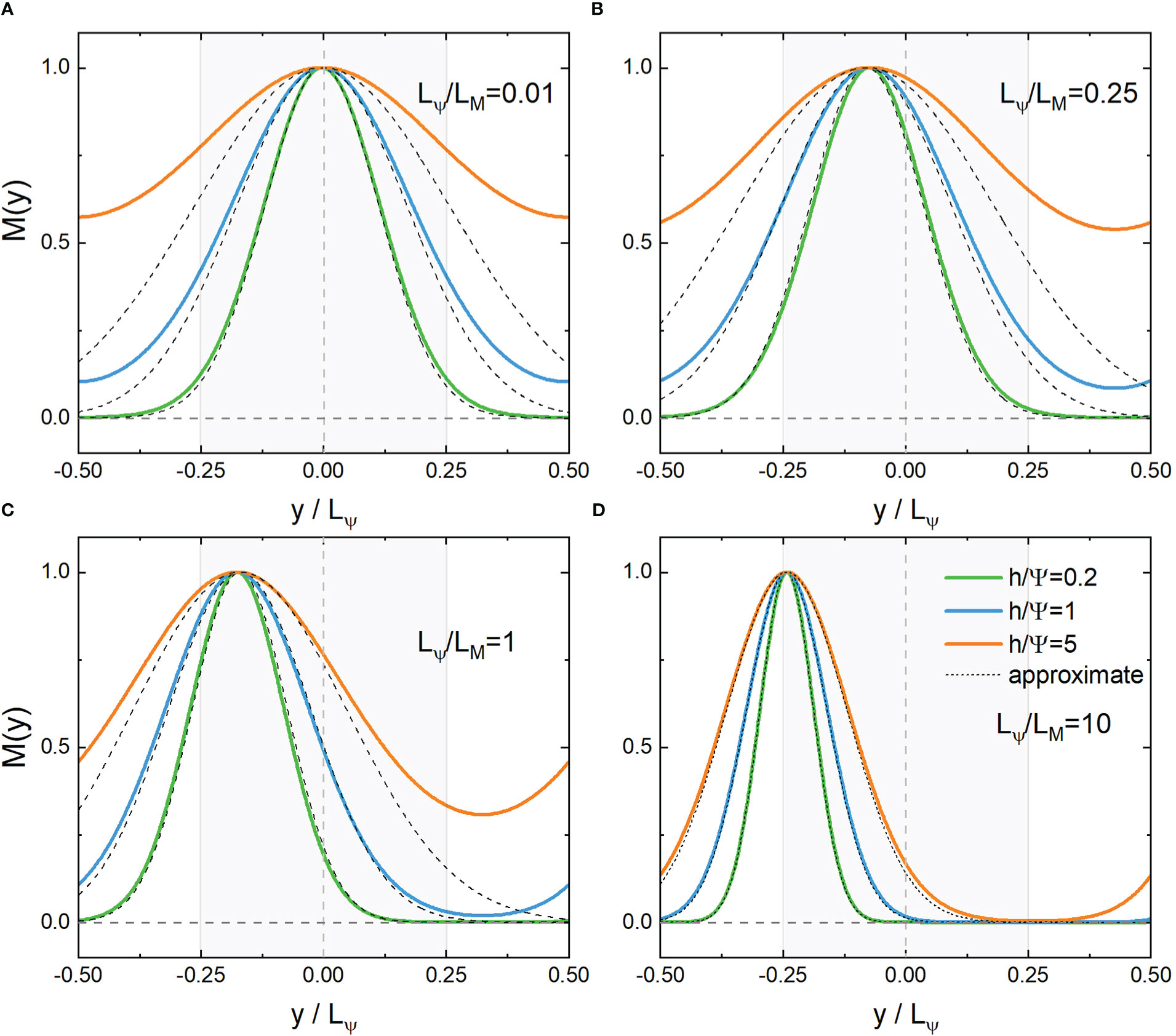
Figure 1 Distribution of the even eigenfunction M_C(ω^′,ξ,y^′) and its approximate solution near the core (y=0) (A, B) or boundary (y/L_Ψ=−1/4) (C, D) with the lowest eigenvalues. L_ψ/L_M=k_x/k₀=0.01,0.25,1,10, $h/\text{Ψ}=\sqrt{2}h{k}_0^2/{\zeta }_0=0.2,1,5$, respectively. Shaded areas indicate negative vorticities.

FIGURE 2

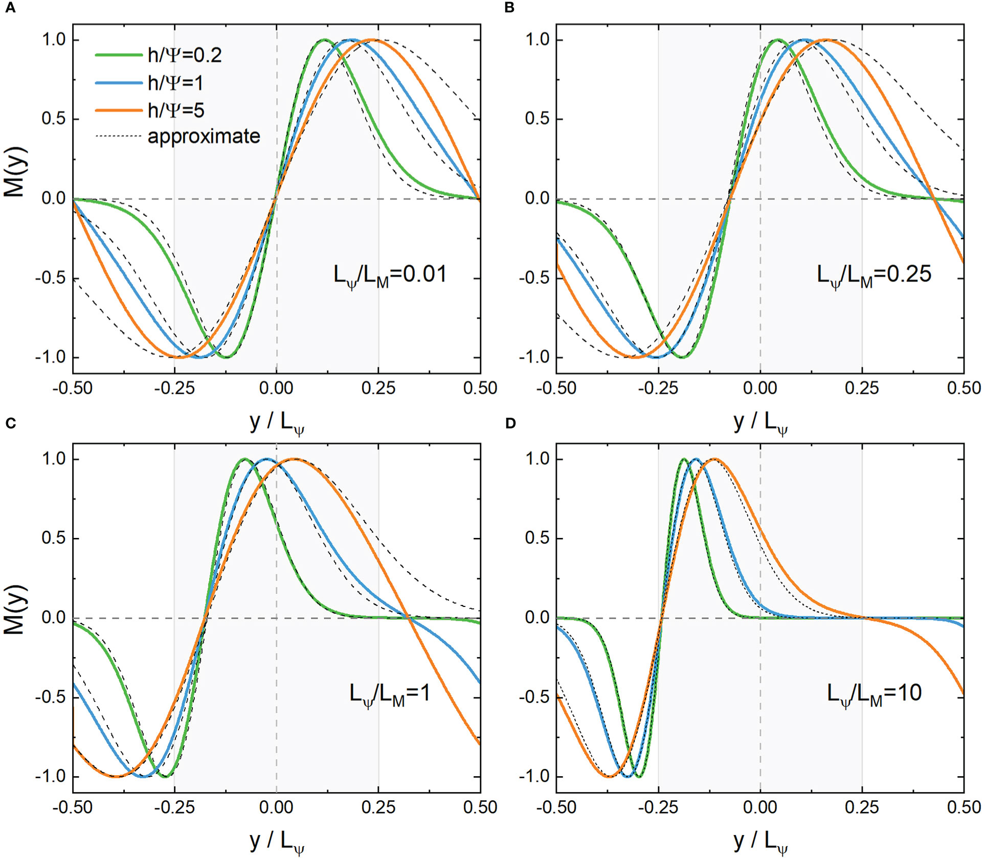
Figure 2 Distribution of the odd eigenfunction M_S(ω^′,ξ,y^′) and its approximate solution near the core (y=0) (A, B) or boundary (y/L_Ψ=−1/4) (C, D) with the lowest eigenvalues. L_ψ/L_M=k_x/k₀=0.01,0.25,1,10 , $h/\text{Ψ}=\sqrt{2}h{k}_0^2/{\zeta }_0=0.2,1,5$, respectively. Shaded areas indicate anticyclones.

FIGURE 3

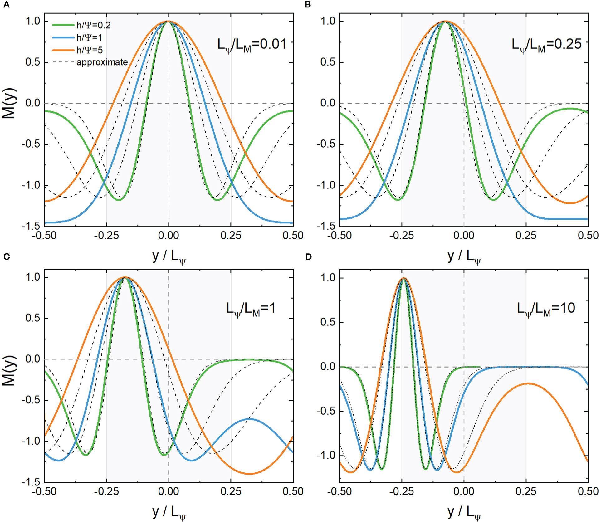
Figure 3 Distribution of the even eigenfunction M_C(ω^′,ξ,y^′) and its approximate solution near the core (y=0) (A, B) or boundary (y/L_Ψ=−1/4) (C, D) with the second lowest eigenvalues. L_ψ/L_M=k_x/k₀=0.01,0.25,1,10, $h/\text{Ψ}=\sqrt{2}h{k}_0^2/{\zeta }_0=0.2,1,5$, respectively. Shaded areas indicate negative vorticities.

FIGURE 4

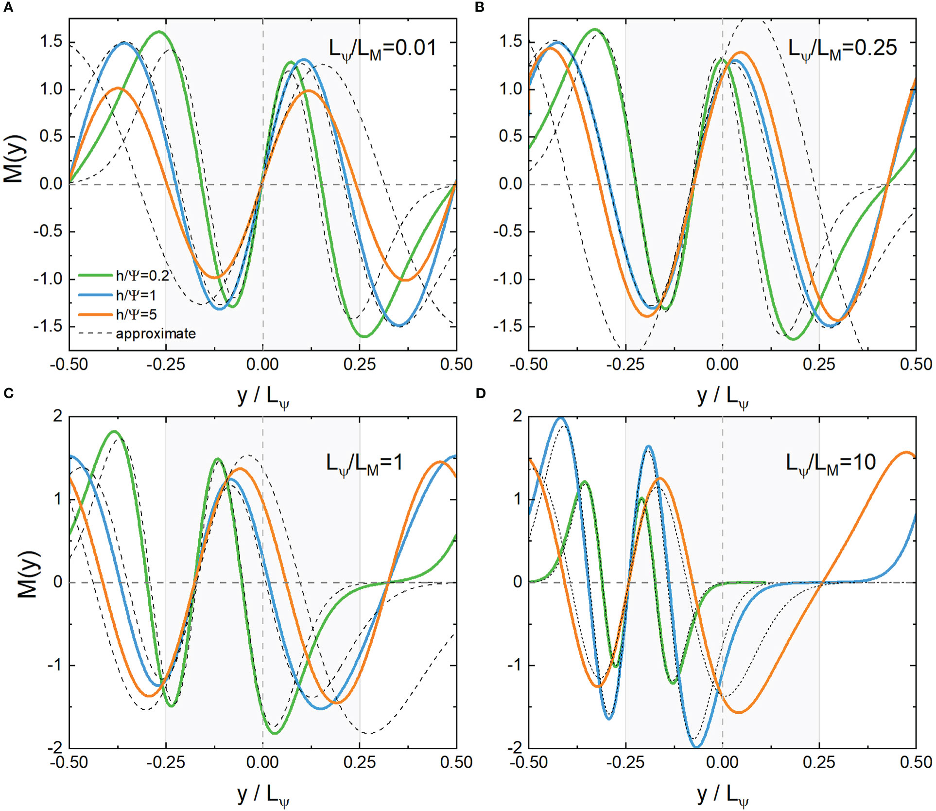
Figure 4 Distribution of the odd eigenfunction M_S(ω^′,ξ,y^′) and its approximate solution near the core (y=0) (A, B) or boundary (y/L_Ψ=−1/4) (C, D) with the second lowest eigenvalues. L_ψ/L_M=k_x/k₀=0.01,0.25,1,10 , $h/\text{Ψ}=\sqrt{2}h{k}_0^2/{\zeta }_0=0.2,1,5$, respectively. Shaded areas indicate anticyclones.

If the original YBJ equation has no advection term, the sine term in Eq.(6) (or φ in Eq.(7)) would be zero, which would result in y_c=0 . Therefore, the scale effect on the deviation from negative vorticity results from advection. The kinetic parameter h/Ψ controls the variance of the wave packet, with smaller h/Ψ≪1 corresponding to more compact wave packets; as h/Ψ increases, the wave packets widen. The oscillatory behavior of the waves grows when the order number of the eigenmodes increases, which would be seen visually by the approximate analytical solutions in the following subsection.

3.1. Approximate solutions near the core of vorticity (L_ψ / L_M ≪ 1)

To see the behavior of the solutions more clearly, we consider approximate solutions near the core of the vorticity where y≈0 , and therefore sin k₀y≈k₀y and $\cos k_{0}y\approx 1-k_0^2{y}^2/2$, then Eq.(6) becomes

$\begin{array}{ll}\frac{h}{2}{\partial }_y^{2}M\left(y\right)+\left({\omega }^{\prime }-a{y}^2+by\right)M=0,& (12)\end{array}$

Where

$\begin{array}{ll}{\omega }^{\prime }=\omega -\frac{h}{2}{k}_x^2+\frac{{\zeta }_0}{2},a=\frac{{\zeta }_0{k}_0^2}{4},b=-{\zeta }_0{k}_x.& (13)\end{array}$

The general solutions with the boundary condition that M(y→∞)→0 are the Parabolic cylinder functions D_n(y) (the branch which is divergent at y→∞ is not shown):

$\begin{array}{ll}M\left(y\right)=C_0 D_n\left[\kappa \left(k_{0}y+\frac{2k_x}{k_0}\right)\right],& (14)\end{array}$

where C₀ is an arbitrary constant, n is a non-negative integer with

$\begin{array}{ll}n=\frac{\sqrt{2}\left(b^2+4a{\omega }^{\prime }\right)}{8\sqrt{a^{3}h}}-\frac{1}{2},\text{\hspace{1em}and\hspace{1em}}\kappa ={\left(2\frac{{\zeta }_0}{h{k}_0^2}\right)}^{1/4}.& (15)\end{array}$

When n is even, D_n(y) is an even function, while when n is odd, D_n(y) is an odd function. The Parabolic cylinder functions can also be represented as:

$\begin{array}{ll}{D}_n\left(y\right)=\frac{1}{2^{n/2}}{e}^{-y^2/4}{H}_n\left(\frac{y}{\sqrt{2}}\right),& (16)\end{array}$

where H_n (y) is the Hermite polynomial of the nth order (Matsuno, 1966). This form is useful because it consists of a Gaussian-type envelope and a fast oscillation. The order number n of the modes appears only in the oscillation part, and the larger n is, the more pronounced the oscillation. The expression (16) gives us an image of the wave’s shape. Since n is a non-negative integer, from Eq.(15) we get the frequency of M (x, y):

$\begin{array}{ll}\omega =\left(\frac{h}{2}-\frac{{\zeta }_0}{k_0^2}\right)k_x^2+\sqrt{\frac{h{\zeta }_0}{8}}\left(1+2n\right)k_0-\frac{{\zeta }_0}{2}.& (17)\end{array}$

From Eq.(14) one can see that the distance between the center of M (y) and the core of negative vorticity, i.e. k₀y_c=−2k_x/k₀ , is proportional to the dimensionless scale factor L_ψ/L_M=|k_x|/k₀ . When L_ψ/L_M≪1 , the waves are trapped near the core of negative vorticities; but for large L_ψ/L_M≫1 , the center of the wave leave the core of negative vorticity. The approximate behavior near the core of vorticity is shown in Figures 1–4 (A, B) which fits well with the exact solutions.

3.2. Approximate solutions near the boundary (for large L_ψ / L_M ≫ 1)

Now we turn to the boundaries between the positive and negative vorticities, where the stream function of the background shear flow can be rewritten as $\psi =\left({\zeta }_0/k_0^2\right)\sin k_0{y}^{\prime }$ with y^′=y+π/2k₀≈0 . Performing a Taylor expansion on ψ and Δψ near the boundary, we get ψ≈(ζ₀/k₀)y^′−ζ₀k₀y^'3/6 , ψ_y^′≈ζ₀/k₀−ζ₀k₀y^'2/2 and Δψ≈−ζ₀k₀y^′ . Under the ansatz M(x,y^′,t)=M(y^′)eⁱ(k_xx−ωt) , the YBJ equation becomes

$\begin{array}{ll}\frac{h}{2}{\partial }_{y\prime }^{2}M+\left({\omega }^{\prime }-a{y}^{\prime 2}+{by}^{\prime }\right)M=0,& (18)\end{array}$

Where

$\begin{array}{ll}{\omega }^{\prime }=\omega -\frac{h}{2}{k}_x^2+\frac{{\zeta }_0{k}_x}{k_0}, a=\frac{{\zeta }_0{k}_0{k}_x}{2}, b=\frac{{\zeta }_0{k}_0}{2}.& (19)\end{array}$

The general solutions with the boundary condition M(y^′→∞)→0 are (the branch which is divergent at y^′→∞ is not shown)

$\begin{array}{ll}M\left(y\right)=C_0 D_n\left[\kappa \left(k_0{y}^{\prime }-\frac{k_0}{2k_x}\right)\right],& (20)\end{array}$

Where

$\begin{array}{ll}n=\frac{8{\omega }^{\prime }{k}_x+{\zeta }_0{k}_0}{8\sqrt{{\zeta }_{0}h{k}_0{k}_x}{k}_x}-\frac{1}{2},\text{\hspace{1em}and\hspace{1em}}\kappa =\sqrt{2}{\left(\frac{{\zeta }_0{k}_x}{h{k}_0^3}\right)}^{1/4}.& (21)\end{array}$

There is a chiral selectivity between the wave number and the vorticity near the boundaries that k_xζ₀>0 , while the opposite case k_xζ₀<0 corresponds to a branch which diverges at y^′→∞ . The approximate behavior near the boundary of vorticity is also shown in Figures 1–4 (C, D) which fits well with the exact solutions. Since n is a non-negative integer, from Eq.(21) we get the frequency of M(x,y):

$\begin{array}{ll}\omega =\frac{h}{2}{k}_x^2-\frac{{\zeta }_0}{k_0}{k}_x+\frac{1+2n}{2}\sqrt{{\zeta }_{0}h{k}_0{k}_x}-\frac{{\zeta }_0{k}_0}{8k_x}.& (22)\end{array}$

3.3. Scale effect emerging from the analytical solutions

In Figure 5, we plot the lowest eigenvalues of M(x,y) from both the Mathieu functions and their approximations near the core and boundaries of the negative vorticity. When k_x=k₀/2 , Eq.(17) and Eq.(22) provide the same result. The approximation near the core of vorticity works if L_ψ/L_M=k_x/k₀≪1/2 , while when L_ψ/L_M=k_x/k₀≫1/2 , the approximation near the boundary is more suitable. Moreover, when h/Ψ increases, the variance of the wave packet in Eqs. (14, 20) increases, and the dispersion term $h{k}_x^2/2$ in Eqs. (17, 22) plays a more important role, changing the convexity of the spectral curve in Figure 5. The frequencies obtained from the approximation near the core of the vorticity are not too accurate because the wave scale is large when k_x→0 , which reduces the localization of the wave.

FIGURE 5

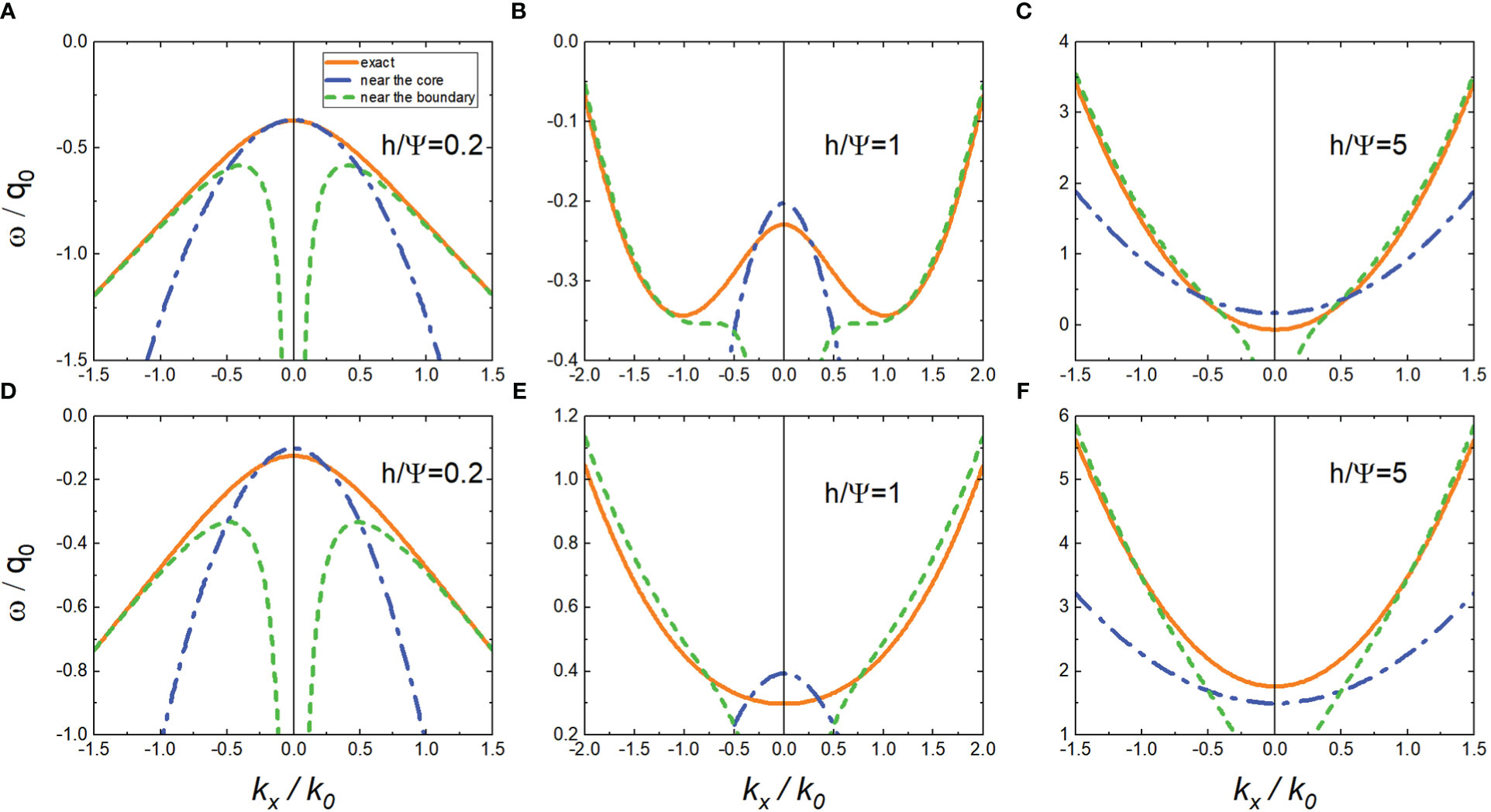
Figure 5 Dispersion relation of the lowest eigenvalues of M_C(ω^′,ξ,y^′) (A–C) and M_S(ω^′,ξ,y^′) (D–F) with $h/\text{Ψ}=\sqrt{2}h{k}_0^2/{\zeta }_0=0.2,1,5$, respectively.

The difference in the approximate behavior at the vorticity core and the boundary is also manifested in the distance between the wave center and the vorticity core, y_c , whose dependence on L_ψ/L_M is shown in Figure 6A. Near the core, y_c is proportional to L_ψ/L_M , while near the boundary, (L_ψ/4−y_c) is inversely proportional to L_ψ/L_M . Thus, a large wave scale benefits the NIW’s concentration.

FIGURE 6

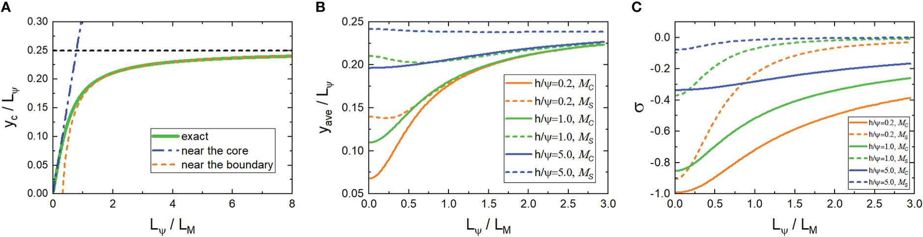
Figure 6 (A) The distance y_c between the center of the waves and the core of the negative vorticity as a function of L_ψ/L_M , which is caused by the advection term. (B, C) y_ave/L_ψ (B) and σ (C) vs L_ψ/L_M from the lowest eigenmodes of M_C and M_S with different h/Ψ=0.2,1,5, respectively.

We define a mean distance y_ave of the NIWs to the core of the negative vorticity y=0 as

$\begin{array}{ll}{y}_{ave}=\frac{{\int }^{}\left|y\right|{\left|M\right|}^{2}dy}{{\int }^{}{\left|M\right|}^{2}dy},& (23)\end{array}$

with which the dimensionless ratio y_ave/L_ψ can be used to measure the concentration of NIWs, as shown in Figure 6B. y_ave increases as L_ψ/L_M increases, which is consistent with the behavior of y_c shown in Figure 6A. However, y_ave grows as h/Ψ increases, while the center of the eigenfunction y_c is independent of h/Ψ.

The scale effect can also be measured by the energy difference of NIWs between the positive and negative vorticities:

$\begin{array}{ll}\sigma =\frac{e_P-e_N}{e_P+e_N},& (24)\end{array}$

where e_P (e_N ) is wave energy in the region with positive (negative) vorticity:

$\begin{array}{ll}{e}_P={\int }^{}{\int }^{}|M{|}^{2}H\left(△\psi \right)dxdy\text{\hspace{1em}and\hspace{1em}}{e}_N={\int }^{}{\int }^{}|M{|}^{2}H\left(-△\psi \right)dxdy.& (25)\end{array}$

Here, H is the Heaviside function. When σ<0 (>0) , the NIWs concentrate in the negative (positive) vorticities. A plot of σ is presented in Figure 6C from the lowest eigenmodes of M_C and M_S , exhibiting the same positive correlation on L_ψ/L_M as in Figures 6 (A, B) Small h/Ψ and L_ψ/L_M refer to a “trapping” regime.

As L_ψ/L_M increases, the advection overtakes the refraction, weakening the capture. When in the “strong dispersion” regime, where h/Ψ≫1 , the concentration becomes insignificant. Besides, the even function M_C has a stronger concentration than the odd M_S .

4. Scale effect in a vortex quadrupole

With the help of the revelation from the above analytical solutions, we study the scale effect of NIWs further in a doubly sinusoidal vortex quadrupole whose streamfunction reads

$\begin{array}{ll}\psi =-\left({\zeta }_0/k_0^2\right)\sin k_{0}x\sin k_{0}y,& (26)\end{array}$

where ζ₀>0 . Thus, the spatial scale is L_ψ=2π/k₀ .

For a given background field, we can obtain the eigenmodes of the system by a finite difference method, as shown in Figure 7. As can be seen from the figure, low-order modes concentrate near the core of anticyclones (Figures 7A, B), while high-order ones can concentrate near the boundaries or the saddle points (Figures 7C, D). For each eigenmode, we define the mean radius

FIGURE 7

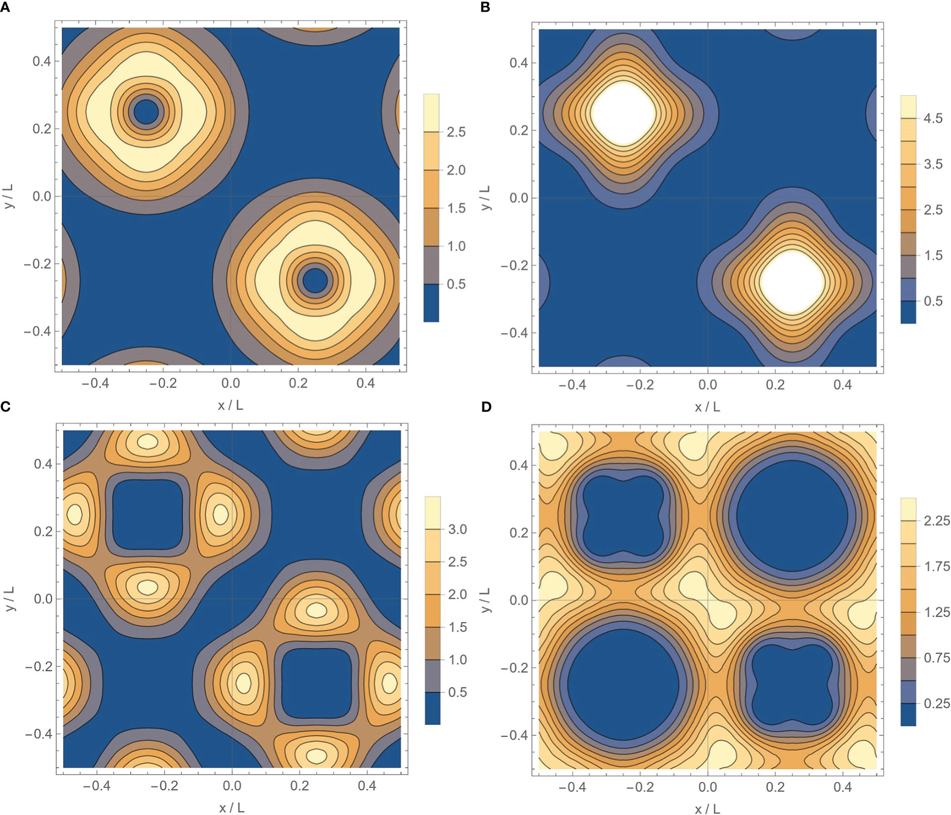
Figure 7 (A–D) Typical eigenmodes in the vortex quadrupole with order number n=1,4,8,9 , respectively. In (A, B), the NIWs concentrate in anticyclones; in (C) they concentrate near the boundaries; while in (D), they concentrate at the saddle points. h/Ψ=1 , L=L_ψ=2π/k₀.

r_ave of NIWs concentrated in anticyclones as

$\begin{array}{ll}{r}_{ave}=\frac{{\int }_{-L_{\psi }/2}^0{\int }_0^{L_{\psi }/2}\sqrt{{(x-x_0)}^2+{(y-y_0)}^2}|M{|}^{2}dxdy}{{\int }_{-L_{\psi }/2}^0{\int }_0^{L_{\psi }/2}|M{|}^{2}dxdy},& (27)\end{array}$

in which the core of the anticyclone (x₀,y₀) locates at (L_ψ/4,−L_ψ/4). We use the dimensionless ratio r_ave/L_ψ to measure the concentration of NIWs, and it depends on the parameter h/Ψ and the order number of the eigenmodes. In Figure 8A we plot r_ave/L_ψ of the eigenmodes with low frequency for different h/Ψ, and the corresponding spatial scale L_ψ/L_M is calculated according to Eq.(4). There is a clear positive correlation between r_ave/L_ψ and L_ψ/L_M , consistent with the trend of y_c and y_ave given by the analytical solutions shown in Figures 6 (A, B). Hence, a larger L_M is associated with a more concentrated NIW in anticyclone for a fixed background vortex quadrupole. It should be noted in Figure 8A that for each h/Ψ, a minimum value of L_ψ/L_M appears, which is inversely correlated with h/Ψ and determined by the most concentrated mode of the system.

FIGURE 8

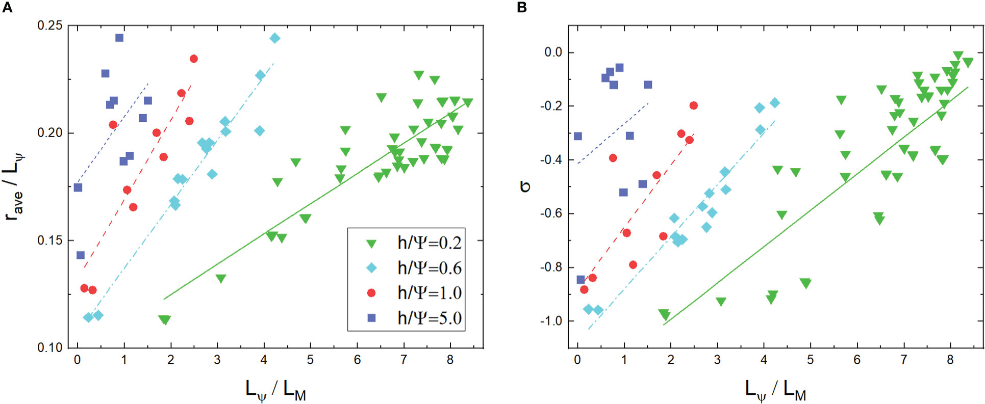
Figure 8 (A) r_ave/L_ψ vs L_ψ/L_M from the eigenmodes with low frequency whose σ<0. (B) σ vs L_ψ/L_M from the eigenmodes with lower frequency whose σ<0 . $\psi =-\left({\zeta }_0/k_0^2\right)\sin k_{0}x\sin k_{0}y$. h/Ψ=0.2,0.6,1,5 , respectively. The lines are obtained by least-square fitting.

Using Eq.(24), we can define the degree of energy concentration σ . Figure 8B also shows that a large wave scale facilitates the concentration. Moreover, a color map of σ as a function of h/Ψ and L_ψ/L_M is shown in Figure 9. With small h/Ψ and L_ψ/L_M, there is a “trapping” regime with a deep negative σ . When h/Ψ or L_ψ/L_M is large enough, the concentration of waves in anticyclones becomes insignificant.

FIGURE 9

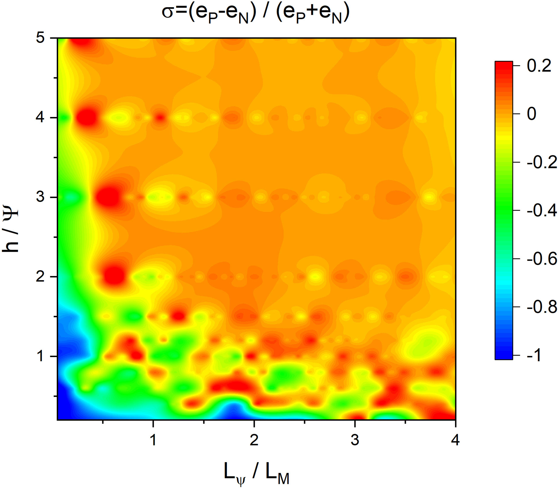
Figure 9 σ=(e_P−e_N)/(e_P+e_N) from the first 120 eigenmodes as a map of h/Ψ and L_ψ/L_M.

With the initial state of the velocity field set as

$\begin{array}{ll}M\left(x,y,t=0\right)=\left(1+i\right)\cos (n{k}_{0}x)\cos (n{k}_{0}y),& (28)\end{array}$

where n is an adjustable parameter, we investigate the long-time (more than 30 days) behavior of NIWs. We plot the time average across the second half of the simulation (about 15-30 days) of r_ave/L_ψ and σ as a function of L_ψ/L_M in Figure 10. A similar scale effect emerges that the concentration of NIW favors larger wavelength L_M defined from Eq.(4). Typically, a larger initial wavelength gives a larger L_M, resulting in a greater concentration. When L_ψ/L_M is large enough, the NIWs are no longer concentrated in anticyclones but tend to the boundary, which leads to a saturation of r_ave/L_ψ and σ, which resembles the results shown by the analytical solutions presented in Figure 6. When h/Ψ increases, the dispersion is enhanced, weakening the concentration of the waves in anticyclones. Note that r_ave/L_ψ=0.25 is the vorticity boundary. Considering the dispersed distribution of M, r_ave/L_ψ can hardly reach the minimum value of 0 or the maximum value of 0.25.

FIGURE 10

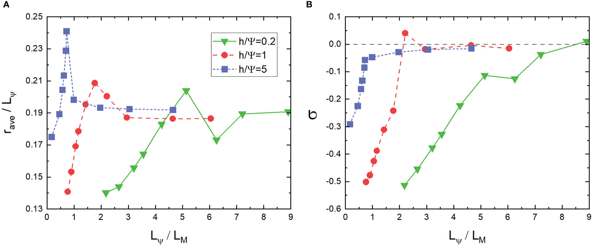
Figure 10 (A) r_ave/L_ψ vs L_ψ/L_M from the long-time average of M(x,y,t). (B) σ vs L_ψ/L_M from the long-time average of M(x,y,t). $\psi =-\left({\zeta }_0/k_0^2\right)\sin k_{0}x\sin k_{0}y$. h/Ψ=0.2,1,5, respectively.

5. Scale effect in random vortexes

To be more realistic, we explore the scale effect of NIWs in the random vortexes, with Gaussian covariance (cf. Danioux et al., 2015). The amplitude scale Ψ of the stream function ψ is defined as its root-mean-square. The numerical simulation of the YBJ equation is carried out on a doubly periodic 256×256 grid of a domain size 4π×4π using the pseudo-spectrum method. In order to ensure numerical stability, a weak biharmonic dissipation ν=10⁻¹⁰ is introduced. Figures 11 (A, B) shows the streamfunction and the associated vorticity field.

FIGURE 11

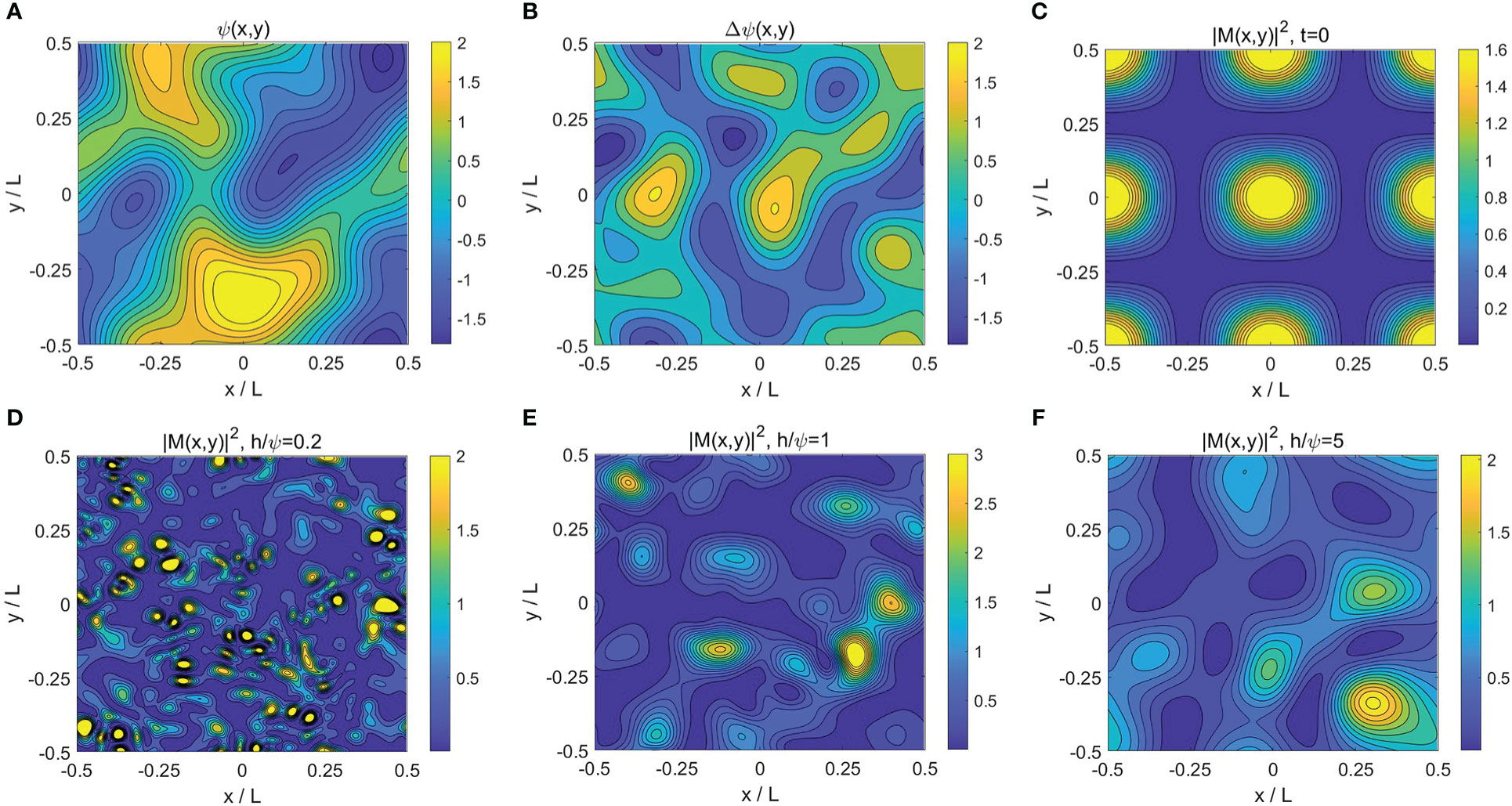
Figure 11 (A, B) Density plots of the random stream function (A) and associated vorticity field (B) with h/Ψ=1. (C) The initial condition for the velocity field, as set in Eq.(28) with n=1. (D–F) The long-time evolutionary behaviors of NIWs with different h/Ψ=0.2,1,5, respectively. The domain size is L=4π.

Because it is not easy to directly get the spatial scale L_Ψ of the random streamfunction, we define the local wavenumber of ψ as

$\begin{array}{ll}{\mathit{\text{k}}}_{\psi }=\frac{\nabla \psi }{\psi }.& (29)\end{array}$

So an averaged local wavenumber $\overline{k_{\psi }}$ is then given as

$\begin{array}{ll}\overline{{\mathit{\text{k}}}_{\psi }}=\frac{{\int }^{}{\int }^{} \left|k_{\psi }\right|{\left|\psi \right|}^{2}dxdy}{{\int }^{}{\int }^{}{\left|\psi \right|}^{2}dxdy},& (30)\end{array}$

which corresponds to the spatial scale $L_{\text{Ψ}}=2\pi /\overline{k_{\psi }}$.

With an initial wave field described by Eq.(28) and illustrated in Figure 11C, the long-time (more than 30 days) behaviors of NIWs are plotted in Figures 11 (D–F) for different h/Ψ . For a larger h/Ψ , the long-time evolution yields a larger saturation scale L_M on average, which is consistent with the result in Danioux et al. (2015) for a homogeneous initial condition M(x,y,t=0)=C where C is a non-zero constant. When h/Ψ is fixed, i.e. for a steady background field, one can find the same positive correlation between the energy concentration σ and the scale factor L_ψ/L_M defined from Eq.(4), as shown in Figure 12. Danioux et al. (2015) argues that NIWs are most concentrated in anticyclones when h/Ψ∼1. However, we point out that this depends on the wave scale in the initial condition and, therefore, on the saturation scale of the wave under long-time evolution. When h/Ψ=5 which belongs to the “strong dispersion” regime, the geostrophic flow has little effect on NIWs, and the concentration of NIWs in anticyclones is reduced. Correspondingly, the scale effect of concentration becomes less obvious. When h/Ψ=0.2 , the system enters the “strong advection” regime with a large L_ψ/L_M≈10 and a weak concentration σ∈(−0.1,0) , which is not presented in the figure.

FIGURE 12

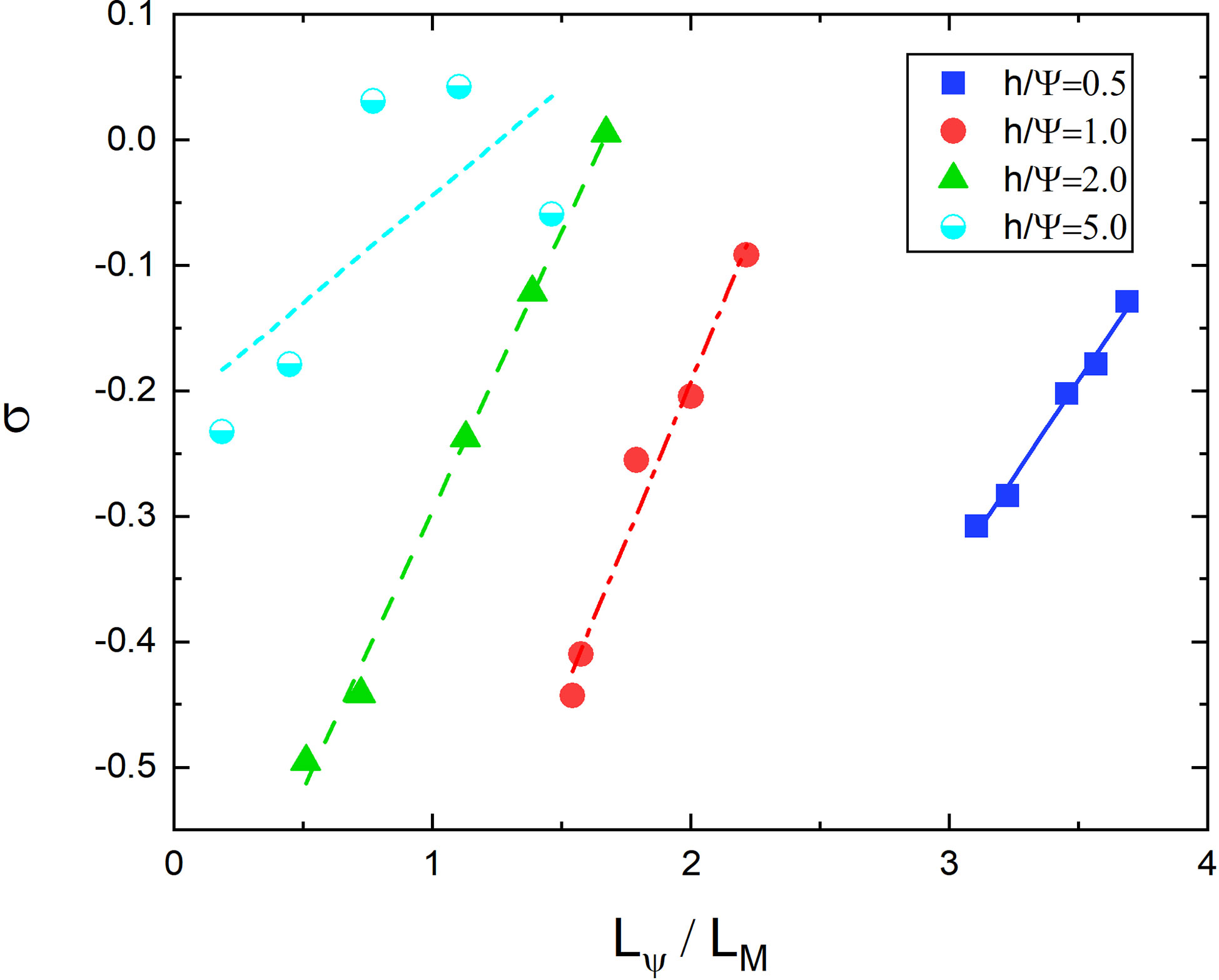
Figure 12 σ vs L_ψ/L_M from the long-time average of M(x,y,t) with h/Ψ=0.5,1,2,5, respectively. The lines are obtained by least square fitting as references.

6. Conservation law and uncertainty relation of NIWs

By analogy with the Schrödinger equation, the YBJ equation can be rewritten as

$\begin{array}{ll}ih{\partial }_{t}M=\widehat{H}M,& (31)\end{array}$

where the Hamiltonian-like operator $\widehat{H}$ reads

$\begin{array}{ll}\widehat{H}=\widehat{H_1}+\widehat{H_2}+\widehat{H_3},& (32)\end{array}$

with

$\begin{array}{ll}\widehat{H_1}=-\frac{h^2}{2}{\nabla }^2, \widehat{H_2}=\frac{h\Delta \psi }{2}, \widehat{H_3}=-ih\left({\psi }_x{\nabla }_y-{\psi }_y{\nabla }_x\right).& (33)\end{array}$

When $\widehat{H_3}=0$, one obtains the Schrödinger equation that governs the complex wave function M(x,y,t) for a single particle with unit mass and external potential hΔψ/2 . Similar to the conservation of energy for particles, i.e. ${\partial }_t\int \int M^{*}\widehat{H}Mdxdy=0$, one can prove that the equation has the following conservation law using properties of the Jacobian and integrating by parts [Danioux et al. (2015)]:

$\begin{array}{ll}\frac{d}{dt}\left(I_1+I_2+I_3\right)=0,& (34)\end{array}$

Where

$\begin{array}{ll}{I}_1=\frac{h^2}{2}\int \int {|\nabla M|}^{2}dxdy, I_2=\frac{h}{2}\int \int \text{Δ}\psi {\left|M\right|}^{2}dxdy, I_3=ih\int \int \psi J\left(M^{*},M\right)dxdy.& (35)\end{array}$

Here, I₁ is non-negative, I₂ is the covariance between Δψ and |M|² reflecting the concentration of NIW energy, and I₃ is an effect of the advection.

In analogy to quantum mechanics, we define the position and momentum operators as

$\begin{array}{ll}\widehat{\mathit{\text{r}}}=\left(x,y\right)\text{\hspace{1em}and\hspace{1em}}\widehat{\mathit{\text{p}}}=-ih\left({\nabla }_x,{\nabla }_y\right).& (36)\end{array}$

Analogously to the uncertainty relation of matter waves, we obtain

$\begin{array}{ll}\sqrt{\langle {(\text{Δ}\widehat{\mathit{\text{r}}})}^2\rangle \langle {(\text{Δ}\widehat{\mathit{\text{p}}})}^2\rangle }\ge \frac{h}{2},& (37)\end{array}$

where $\widehat{A}$ denotes the weighted average following $\int \int M^{*}\widehat{A}Mdxdy$, and $\text{Δ}\widehat{\mathit{\text{r}}}$ and $\text{Δ}\widehat{\mathit{\text{p}}}$ are defined as

$\begin{array}{ll}\text{Δ}\widehat{\mathit{\text{r}}}\equiv \widehat{\mathit{\text{r}}}-\langle \widehat{\mathit{\text{r}}}\rangle , \text{Δ}\widehat{\mathit{\text{p}}}\equiv \widehat{\mathit{\text{p}}}-\langle \widehat{\mathit{\text{p}}}\rangle .& (38)\end{array}$

The weighted averages $\langle {(\text{Δ}\widehat{\mathit{\text{r}}})}^2\rangle$ and $\langle {(\text{Δ}\widehat{\mathit{\text{p}}})}^2\rangle$ are used to measure the uncertainty in position and momentum, acting like the variance of a data set. If $\langle {(\text{Δ}\widehat{\mathit{\text{r}}})}^2\rangle$ ($\langle {(\text{Δ}\widehat{\mathit{\text{p}}})}^2\rangle$) gets smaller, we learn that the waves become more concentrated in position (momentum) space. The uncertainty relation (37) tells us that the waves cannot be overly concentrated simultaneously in both position and momentum spaces, which is a natural consequence of the Fourier transform.

When the background field traps the waves, i.e. , small $\langle \widehat{\mathit{\text{p}}}\rangle$guaranteeing that the waves do not tend to escape. Then the uncertainty in momentum becomes

$\begin{array}{ll}\langle {(\text{Δ}\widehat{\mathit{\text{p}}})}^2\rangle \approx \langle {\widehat{\mathit{\text{p}}}}^2\rangle =\langle 2\widehat{H_1}\rangle =2I_1.& (39)\end{array}$

Supposing the NIWs are initially uniformly distributed, i.e. I₂=0 . Gradually, the waves become concentrated, corresponding to a decrease in the uncertainty in position $\langle {(\text{Δ}\widehat{\mathit{\text{r}}})}^2\rangle$, and then the uncertainty in momentum $\langle {(\text{Δ}\widehat{\mathit{\text{p}}})}^2\rangle$ increases according to Eq.(37). Thus, I₁ increases according to Eq.(39). When L_ψ/L_M≫1 , one gets I₃≫I₂ according to a scaling analysis of Eq.(35). This corresponds to the “strong advection” regime where the NIW’s concentration is insignificant. On the contrary, when L_ψ/L_M≪1 , we have I₂≫I₃ , and the conservation law implies that an increase in I₁ leads to negative I₂ . Thus, when large-scale NIWs are concentrated, the uncertainty relation guides them to concentration in anticyclones. This scale-dependent of NIW’s concentration is inconsistent with our analytical and numerical results presented in Section 4–6.

7. Conclusion and discussion

Based on the YBJ equation, we analyze the scale effect of NIW’s concentration by both analytical derivations and numerical simulations. We start from the exact and approximate solutions for a sinusoidal background shear flow and indicate that a larger wave scale facilitates the concentration. The particular forms of approximate solutions, consisting of envelopes and order-dependent oscillations, give us intuitions about the wave shapes and approximate frequency expressions. Numerical simulations with background vortex quadrupoles and random vortexes confirm the large scale’s preference in enhancing the NIW’s concentration.

Based on the two dimensionless parameters, h/Ψ and L_ψ/L_M , in the YBJ equation, we classify three dynamic regimes: a strong “dispersion” regime with h/Ψ≫1 , a “trapping” regime with small h/Ψ and L_ψ/L_M, and an “advection” regime with a small h/Ψ and a large L_ψ/L_M . Figure 13 illustrates this classification. It is worth noting that for each h/Ψ , there exists a minimum value for L_ψ/L_M , which is determined by the scale of the most concentrated eigenmode of the system. Moreover, the smaller h/Ψ is, the larger the minimum will be. Unlike in Danioux et al. (2015), where with a homogeneous initial state, they attribute the energy concentration to the effect of only one parameter h/Ψ , we consider variable initial conditions and obtain a phase diagram about h/Ψ and L_ψ/L_M , which leads to a classification of “advection” regime.

FIGURE 13

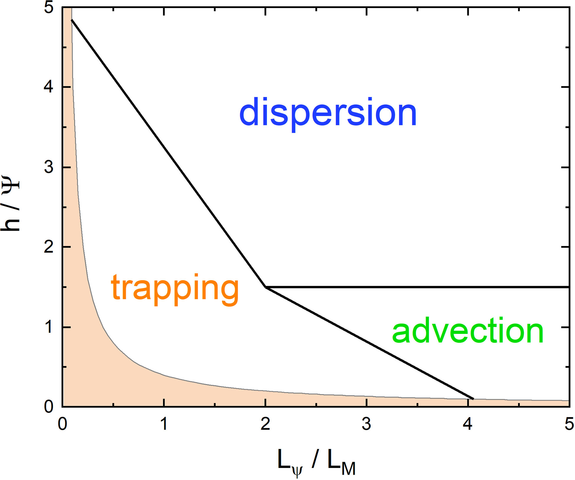
Figure 13 Schematic diagram of the regime classification. The shaded part is the forbidden area of the system, which is determined by the scale of the most concentrated eigenmode.

The scale effect works mainly in the “trapping” regime. When NIWs concentrate in negative vorticities, their centers do not coincide precisely with the core of the vorticities, leaving a displacement originating from the advection. For strong “trapping”, this displacement is proportional to the local wavenumber; However, when the advection effect becomes stronger, waves approach the boundaries between positive and negative vorticities, and the displacement is inversely proportional to the local wavenumber. Thus, the advection prevents the concentration of NIWs, and NIWs with large local wavenumbers (small scales) are more likely to appear at the boundaries. As small-scale structures continue to increase, the system enters a “strong advection” regime. In contrast to the two regimes mentioned above, in the “strong dispersion” regime, NIWs quickly disperse and are slightly influenced by the background vorticity. Therefore, the concentration of the NIWs is very weak in the “strong advection” and “strong dispersion” regimes (Llewellyn Smith, 1999).

Based on the similarity between the YBJ equation to the Schrödinger equation (Balmforth et al., 1998; Danioux et al., 2015), we present a new perspective for the NIW’s concentration in the anticyclone using the uncertainty principle in quantum mechanics. Ignoring the advection term, these two equations are identical, so considering the higher probability of the particle being in the lower potential region, the NIWs prefer to concentrate in negative relative vorticities. Considering the advection’s effect, which hinders NIW’s concentration, this concentration trend could still be true if the change in the advection-related conservation, I₃ in Eq.35, is small enough. Based on the uncertainty relation, wave concentration means a decrease in the uncertainty of the wave’s position, which leads to an increment in the uncertainty of its momentum. This will enhance the “particle” kinetic-like energy term, defined as I₁ in Eq.35. Then, due to the conservation of energy, it could reduce the vorticity-related energy term if |ΔI₃|<ΔI₁ , leading the concentration towards negative vorticities. Thus, a link between the down-scale waves in space and the distribution of energy in anticyclones is naturally established.

We only consider some modes with low frequencies when studying eigenmodes in the sinusoidal shear flow and vortex quadrupole. This is reasonable because they contribute the most to the mode projection of a realistic initial condition (Balmforth et al. (1998)). For the low-frequency solutions, corresponding to small wavenumbers, the center of symmetry of the solutions can be regarded as the center of the energy distribution. While, for the modes with high frequencies, the Riemann-Lebesgue Lemma implies that the strong spatial oscillation induces only weak concentration if there is any. In addition, too high a frequency is already far from the near-inertial regime, which may make the YBJ equation invalid.

Data availability statement

The raw data supporting the conclusions of this article will be made available by the authors, without undue reservation.

Author contributions

FZ conducted the analytical derivations and numerical simulations, and wrote the first draft of the manuscript. J-HX conceived the idea and revised the manuscript. All authors contributed to the article and approved the submitted version.

Funding

This research was supported by the National Natural Science Foundation of China (NSFC) under grant no. 92052102 and 12272006, and the Joint Laboratory of Marine Hydrodynamics and Ocean Engineering, Pilot National Laboratory for Marine Science and Technology (Qingdao) under grant no. 2022QNLM010201.

Acknowledgments

The authors thank ShenHua Wang for his careful reading of the manuscript and his suggestions for revisions.

Conflict of interest

The authors declare that the research was conducted in the absence of any commercial or financial relationships that could be construed as a potential conflict of interest.

Publisher’s note

All claims expressed in this article are solely those of the authors and do not necessarily represent those of their affiliated organizations, or those of the publisher, the editors and the reviewers. Any product that may be evaluated in this article, or claim that may be made by its manufacturer, is not guaranteed or endorsed by the publisher.

References

Alford M. H. (2001). Internal swell generation: The spatial distribution of energy flux from the wind to mixed layer near-inertial motions. J. Phys. Oceanography 31, 2359–2368. doi: 10.1175/1520-0485(2001)031<2359:ISGTSD>2.0.CO;2

CrossRef Full Text | Google Scholar

Alford M. H., MacKinnon J. A., Simmons H. L., Nash J. D. (2016). Near-inertial internal gravity waves in the ocean. Annu. Rev. Mar. Sci. 8, 95–123. doi: 10.1146/annurev-marine-010814-015746

CrossRef Full Text | Google Scholar

Balmforth N. J., Smith S. G. L., Young W. R. (1998). Enhanced dispersion of near-inertial waves in an idealized geostrophic flow. J. Mar. Res. 56, 1–40. doi: 10.1357/002224098321836091

CrossRef Full Text | Google Scholar

Danioux E., Klein P., Rivière P. (2008). Propagation of wind energy into the deep ocean through a fully turbulent mesoscale eddy field. J. Phys. Oceanography 38, 2224–2241. doi: 10.1175/2008JPO3821.1

CrossRef Full Text | Google Scholar

Danioux E., Vanneste J., Bühler O. (2015). On the concentration of near-inertial waves in anticyclones. J. Fluid Mechanics 773, R2. doi: 10.1017/jfm.2015.252

CrossRef Full Text | Google Scholar

D’Asaro E. A., Eriksen C. C., Levine M. D., Paulson C. A., Niiler P. P., Meurs P. V. (1995). Upper-ocean inertial currents forced by a strong storm. part i: Data and comparisons with linear theory. J. Phys. Oceanography 25, 2909–2936. doi: 10.1175/1520-0485(1995)025<2909:UOICFB>2.0.CO;2

CrossRef Full Text | Google Scholar

Elipot S., Lumpkin R., Prieto G. (2010). Modification of inertial oscillations by the mesoscale eddy field. J. Geophysical Research: Oceans 115, (C9). doi: 10.1029/2009JC005679

CrossRef Full Text | Google Scholar

Ferrari R., Wunsch C. (2009). Ocean circulation kinetic energy: Reservoirs, sources, and sinks. Annu. Rev. Fluid Mechanics 41, 253–282. doi: 10.1146/annurev.fluid.40.111406.102139

CrossRef Full Text | Google Scholar

Granata T., Wiggert J. D., Dickey T. D. (1995). Trapped, near-inertial waves and enhanced chlorophyll distributions. J. Geophysical Res. 100, 20793–20804. doi: 10.1029/95JC01665

CrossRef Full Text | Google Scholar

Jochum M., Briegleb B. P., Danabasoglu G., Large W. G., Norton N. J., Jayne S. R., et al. (2013). The impact of oceanic near-inertial waves on climate. J. Climate 26, 2833–2844. doi: 10.1175/JCLI-D-12-00181.1

CrossRef Full Text | Google Scholar

Joyce T. M., Toole J. M., Klein P., Thomas L. N. (2013). A near-inertial mode observed within a gulf stream warm-core ring. J. Geophysical Res. 118, 1797–1806. doi: 10.1002/jgrc.20141

CrossRef Full Text | Google Scholar

Klein P., Smith S. G. L. (2001). Horizontal dispersion of near-inertial oscillations in a turbulent mesoscale eddy field. J. Mar. Res. 59, 697–723. doi: 10.1357/002224001762674908

CrossRef Full Text | Google Scholar

Klein P., Smith S. L., Lapeyre G. (2004). Organization of near-inertial energy by an eddy field. Q. J. R. Meteorological Soc. 130, 1153–1166. doi: 10.1256/qj.02.231

CrossRef Full Text | Google Scholar

Klein P., Tréguier A. M. (1995). Dispersion of wind-induced inertial waves by a barotropic jet. J. Mar. Res. 53, 1–22. doi: 10.1357/0022240953213331

CrossRef Full Text | Google Scholar

Kunze E. (1985). Near-inertial wave propagation in geostrophic shear. J. Phys. Oceanography 15, 544–565. doi: 10.1175/1520-0485(1985)015<0544:NIWPIG>2.0.CO;2

CrossRef Full Text | Google Scholar

Kunze E., Sanford T. B. (1984). Observations of near-inertial waves in a front. J. Phys. Oceanography 14, 566–581. doi: 10.1175/1520-0485(1984)014<0566:OONIWI>2.0.CO;2

CrossRef Full Text | Google Scholar

Lee D.-K., Niiler P. P. (1998). The inertial chimney: The near-inertial energy drainage from the ocean surface to the deep layer. J. Geophysical Research: Oceans 103, 7579–7591. doi: 10.1029/97JC03200

CrossRef Full Text | Google Scholar

Llewellyn Smith S. G. (1999). Near-inertial oscillations of a barotropic vortex: trapped modes and time evolution. J. Phys. oceanography 29, 747–761. doi: 10.1175/1520-0485(1999)029<0747:NIOOAB>2.0.CO;2

CrossRef Full Text | Google Scholar

Matsuno T. (1966). Quasi-geostrophic motions in the equatorial area. J. Meteorological Soc. Japan. Ser. II 44, 25–43. doi: 10.2151/jmsj1965.44.125Matsuno1966

CrossRef Full Text | Google Scholar

Rimac A., von Storch J.-S., Eden C., Haak H. (2013). The influence of high-resolution wind stress field on the power input to near-inertial motions in the ocean. Geophysical Res. Lett. 40, 4882–4886. doi: 10.1002/grl.50929Rimac.et.al.2013

CrossRef Full Text | Google Scholar

Rocha C. B., Wagner G. L., Young W. R. (2018). Stimulated generation: extraction of energy from balanced flow by near-inertial waves. J. Fluid Mechanics 847, 417–451. doi: 10.1017/jfm.2018.308Rocha.et.al.2018

CrossRef Full Text | Google Scholar

van Meurs P. (1998). Interactions between near-inertial mixed layer currents and the mesoscale: The importance of spatial variabilities in the vorticity field. J. Phys. Oceanography 28, 1363–1388. doi: 10.1175/1520-0485(1998)028<1363:IBNIML>2.0.CO;2

CrossRef Full Text | Google Scholar

Wang D.-P. (1991). Generation and propagation of inertial waves in the subtropical front. J. Mar. Res. 49, 619–633. doi: 10.1357/002224091784995747

CrossRef Full Text | Google Scholar

Weller R. A. (1982). The relation of near-inertial motions observed in the mixed layer during the jasin, (1978) experiment to the local wind stress and to the quasi-geostrophic flow field. J. Phys. Oceanography 12, 1122–1136. doi: 10.1175/1520-0485(1982)012<1122:TRONIM>2.0.CO;2

CrossRef Full Text | Google Scholar

Xie J.-H. (2020). Downscale transfer of quasigeostrophic energy catalyzed by near-inertial waves. J. Fluid Mechanics 904, A40. doi: 10.1017/jfm.2020.709Xie2020

CrossRef Full Text | Google Scholar

Xie J.-H., Vanneste J. (2015). A generalised-lagrangian-mean model of the interactions between near-inertial waves and mean flow. J. Fluid Mechanics 774, 143–169. doi: 10.1017/jfm.2015.251XieVanneste2015

CrossRef Full Text | Google Scholar

Young W. R., Jelloul M. B. (1997). Propagation of near-inertial oscillations through a geostrophic flow. J. Mar. Res. 55, 735–766. doi: 10.1357/0022240973224283

CrossRef Full Text | Google Scholar

Zhai X., Greatbatch R. J., Zhao J. (2005). Enhanced vertical propagation of storm-induced near-inertial energy in an eddying ocean channel model. Geophysical Res. Lett. 32, (18). doi: 10.1029/2005GL023643

CrossRef Full Text | Google Scholar