Effects of spatial bottom friction parameterization scheme on the tidal dynamics in the macrotidal East China Seas

In this study, the effects of different bottom friction coefficient (BFC) parameterization schemes on the modelling of four principal tidal constituents (M₂, S₂, K₁, O₁ tides) in the macrotidal East China Seas were investigated by using a high-resolution model based on FVCOM (Finite Volume Community Ocean Model). The applied BFC schemes include: the empirical constant (EC-BFC), sediment-dependent form (SD-BFC), and spatial varying BFC obtained from adjoint data assimilation (SV-BFC). The comparisons between the simulated results and the observations from satellite altimeters and tidal gauge stations indicated that the SV-BFC scheme is superior to others. The locations of amphidromic points calculated with EC-BFC and SD-BFC were in the northwest of those from SV-BFC. The variations in tidal dynamics between different BFC schemes were closely related to the spatial distributions of BFCs, especially in high-valued BFC areas, e.g., the West Korea Bay, the South Yellow Sea, and the eastern coasts of Jiangsu, Zhejiang and Fujian provinces. The tidal energy flux transporting into Bohai and Yellow Seas increased under the SV-BFC scheme, while smaller tidal energy flux transporting from the Korea Strait was generated by SV-BFC as compared to those from EC-BFC and SD-BFC. The high-valued BFC areas in the SV-BFC scheme dissipated larger amounts of tidal energy, and the average values of Simpson-Hunter numbers were lower than those with the other two schemes. However, the values of Simpson-Hunter numbers increased in the West Korea Bay and Jianghua Bay with high-valued BFCs because of the decreasing current velocity under the headland-shaped topography.

1 Introduction

The most important sink of oceanic kinetic energy is the bottom boundary layer in shallow seas where intensive dissipation occurs (Munk and Wunsch, 1998; Blakely et al., 2022). The bottom boundary layer (BBL), the interface between the seabed and the overlying water column, is where exchanges of particles (Dyer and Soulsby, 1988; Brink, 2016), chemicals (Huettel et al., 2014), and organisms (Cowen and Sponaugle, 2009) take place. Frictional dissipation of energy and turbulent mixing of mass, momentum, and heat are rather significant in these regions, and thus, the BBL plays an important role in the oceanic momentum balance (McWilliams, 2006; Trowbridge and Lentz, 2018). The dissipation mechanisms for global tides include bottom friction dissipation and internal tide dissipation during the conversion from barotropic to baroclinic tides (Munk, 1997). Global tidal energy dissipation was evaluated to be equal to 3.7 terawatts, and nearly 2.8-3.1 terawatts was allocated to the dissipation in the turbulent BBL of marginal seas (Munk and Wunsch, 1998).

Bottom friction plays an important role in shelf flows, but knowledge about this term is still inadequate. The bottom friction coefficient (BFC) was introduced to parameterize the bottom friction term usually with a quadratic function of the near-bottom current velocity (Mofjeld, 1988; Guo and Yanagi, 1998). In early estimates of bottom friction dissipation by Taylor (1920) and Jeffreys (1921), the bottom friction dissipation depended on the product of the BFC and tidal velocity cubed. Field measurements ensure that BFC is not a universal constant (Cheng et al., 1999; Fan et al., 2019; Bo and Ralston, 2020), i.e. with temporal and spatial variations, and is believed to be one of the main uncertainties for the evaluation of tidal energy dissipation (Munk and Wunsch, 1998). Several methods were suggested to determine the BFC. Zhao et al. (1993) simulated the semidiurnal and diurnal tides and tidal currents in the whole East China Seas with different BFC in different subdomains. By using the depth-dependent form of BFC, Kang et al. (1998) carried out a fine grid tidal modeling experiment to study the tidal phenomena in the Yellow and East China Seas. Pringle et al. (2018) presented a semidata-informed method to estimate spatially varying BFC from seabed and physical properties of the flow. Blakely et al. (2022) used a depth-dependent Manning’s coefficient to optimize the boundary layer friction parameters and estimate the boundary layer dissipation. They concluded that altering friction values in high-energy dissipation areas has significant basin-scale impacts on tidal results. In shallow coastal seas, BFC can be affected by multiple factors (Cheng et al., 1999; Fan et al., 2019; Bo and Ralston, 2020; Qian et al., 2021), which results in the spatiotemporal variations in BFC. The spatiotemporal distributions of BFC had been investigated extensively by parameter estimations based on data assimilation techniques (Das and Lardner, 1991; Lu and Zhang, 2006; Zhang et al., 2011; Gao et al., 2015; Qian et al., 2021; Wang et al., 2021). A more reasonable spatial distribution of BFC of the East China Seas was obtained by assimilating multi-missions satellite altimeter observations into an adjoint tidal model (Qian et al., 2021). The temporal and spatial variations in the estimated BFCs were significantly correlated with the current speed and water depth, which ultimately induce the erosion-deposition of sediments on the seabed (Wang et al., 2021).

Overall, different parameterization schemes of BFC have been used in previous studies (Zhao et al., 1993; Kang et al., 1998; Lee and Jung, 1999; Egbert and Erofeeva, 2002; Egbert et al., 2004; Wang et al., 2014; Pringle et al., 2018; Chu et al., 2021). Wang et al. (2014) investigated the effects of BFC schemes on single-tidal simulation. Chu et al. (2019) studied the sensitivities of modelling storm surge to BFC schemes, and they also investigated the effects of BFC schemes on the modelling of shallow-water tides and tidal duration asymmetry. However, so far there are few systematic comparisons among the different schemes of BFC on the estimation of energy flux, oceanic mixing, and bottom friction dissipation. The goal of this study is to investigate the effects of various schemes of BFC on the tidal dynamics in the macrotidal East China Seas. More specifically, the following tasks will be achieved. Firstly, a high-resolution unstructured model is developed based on FVCOM (Finite Volume Community Ocean Model) to simulate the four principal tidal constituents (M₂, S₂, K₁, and O₁) in the macrotidal East China Seas. Secondly, different schemes of BFC including empirical constant (EC-BFC), sediment-dependent form (SD-BFC), and spatial varying BFC obtained from data assimilation (SV-BFC) are compared. Furthermore, the variations in oceanic energy, mixing and bottom friction dissipation between different BFC schemes are discussed.

The paper is organized as follows. Section 2 introduces the methodology, including the model configuration and experiment settings, and model verifications. Section 3 describes the sensitivity analysis and model results. The discussions are arranged in Section 4. The conclusions are drawn in Section 5.

2 Methodology

2.1 Model development

FVCOM model, with a non-overlapping unstructured triangular grid ideally to resolve dynamics in irregular complex coastlines, is used in this study (Chen et al., 2003; Chen et al., 2007). The model solves the momentum and mass conservation equations in integral form by computing fluxes between nonoverlapping horizontal triangular control volumes. This numerical approach also provides optimal representations of mass, momentum, salinity, and heat conservation in coastal and estuarine regions with complex geometries.

The bathymetry and mesh of the computational domain are shown in Figure 1. The mesh includes parts of the East China Sea to minimize the influence of open boundaries. The land boundary is limited by the coastline, and open boundaries are located in the northern, southern, and eastern parts of the domain. The unstructured triangular grid of the computational domain consists of 29916 nodes and 57125 elements with a spatial resolution of 0.5 km for coastal zones and decreased resolution up to 20 km towards open sea boundaries. In addition, seven uniform σ layers are specified in the vertical profiles. The hydrodynamics in the study area is dominantly driven by currents induced by barotropic tide (Li et al., 2018; Wu et al., 2018). Four principal tidal constituents (M₂, S₂, K₁, and O₁) were used to generate the tidal elevations along the open boundaries. The astronomical tidal constituents along open boundaries were derived from TPXO 7.2 established by the University of Oregon (http://volkov.oce.orst.edu/tides/TPXO7.2.html). The high-resolution bathymetry data for the coastal areas adjacent to Zhejiang province and the Yangtze estuary were provided by the Ocean and Fisheries Bureau of Zhejiang Province. Bathymetry data for areas further offshore were obtained from Etopo1 (https://www.ngdc.noaa.gov/mgg/bathymetry/). All the bathymetry data were interpolated to the computational cells. The Mellor and Yamada level-2.5 turbulence closure scheme is adopted to parameterize the vertical mixing (Mellor and Yamada, 1982). The model used in this study is FVCOM v4.0, while the baroclinic effect is ignored. This model has been successfully applied to numerous estuaries and continental shelf areas (Chu et al., 2019; Zhang et al., 2021).

FIGURE 1

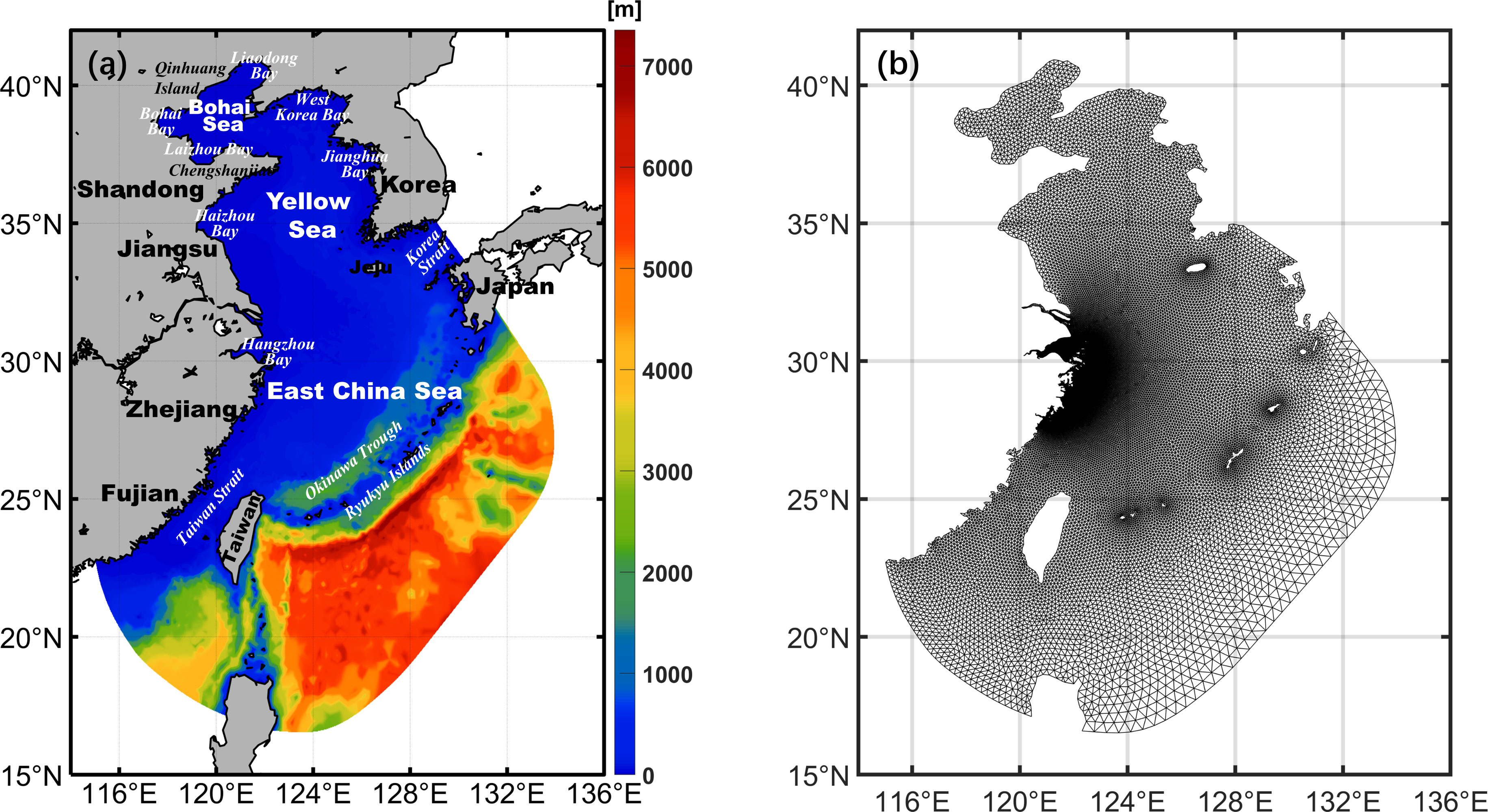
Figure 1 (A) Bathymetry of numerical model, (B) computational grid of study domain.

2.2 Numerical experiments

In this study, three BFC schemes are employed in the FVCOM to simulate the four principal tidal constituents. Generally, the BFC parameterizations can be summarized as: an empirical constant, different constants in different subdomains, depth-dependent form with Chezy coefficient, sediment form, and the spatial varying BFC obtained from data assimilation. Wang et al. (2014) concluded that the simulated M₂ tide in the East China Seas with the first three BFC schemes had larger discrepancies compared with field observations. Therefore, the employed BFC schemes in this study are described as follows.

EXP 1 (EC-BFC): The BFC is treated as a constant in the East China Seas, BFC = 0.0022. (Qian et al., 2021).

EXP 2 (SD-BFC): The BFCs are estimated by the semidata-informed method with the knowledge of seabed sediments and the physical properties of the flow (Pringle et al., 2018) (Figure 2A).

EXP 3 (SV-BFC): The spatially varying BFCs in the East China Seas were obtained by assimilating multi-mission satellite observations from TOPEX/Poseidon, Jason-1, and Jason-2 into a tidal model with an adjoint method (Qian et al., 2021) (Figure 2B).

FIGURE 2

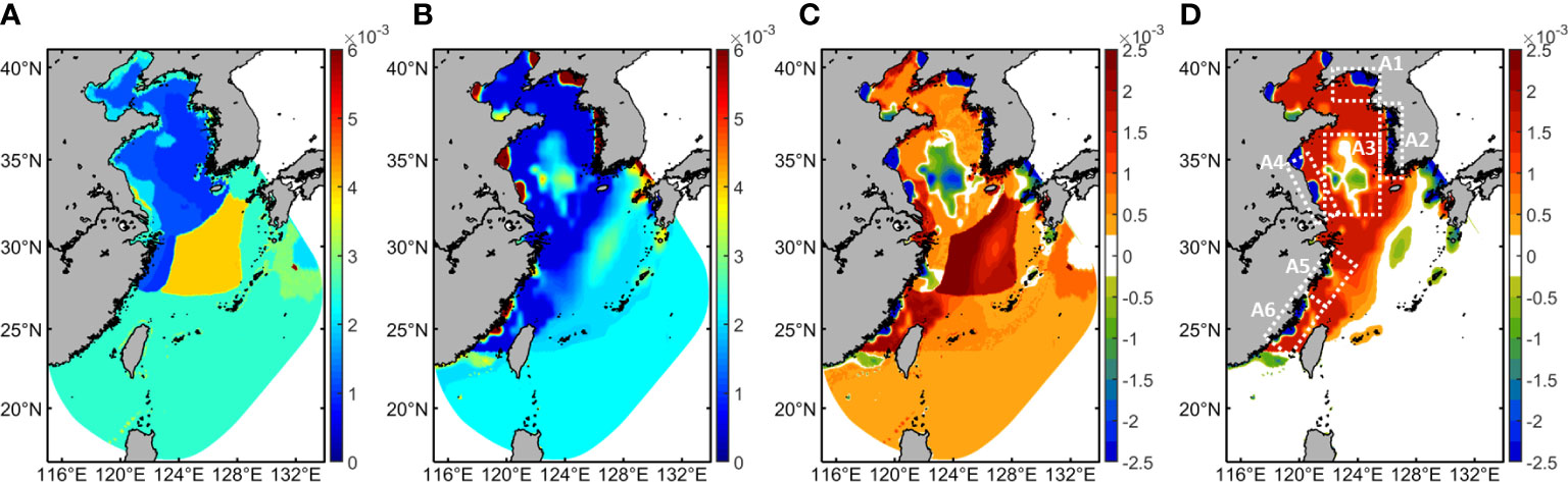
Figure 2 (A, B) Spatial distributions of BFCs of EXP 2 and EXP 3, respectively. (C) Differences between the BFCs of EXP 2 and those of EXP 3 (BFC_EXP2 – BFC_EXP3). (D) Differences between the BFCs of EXP 1 and those of EXP 3 (BFC_EXP1 – BFC_EXP3). White dashed boxes mark the areas of the Korea Bay (A1), the Jianghua Bay (A2), the middle South Yellow Sea (A3), and the eastern coasts of Jiangsu (A4), Zhejiang (A5) and Fujian provinces (A6).

The spatially varying bottom friction coefficient data of the SD-BFC scheme and SV-BFC scheme were interpolated into the computational cells. The model was launched with a cold start. With the assumption of zero heat flux, the simulation time of the model lasted from 1 February 2012 to 31 March 2012, and the modeling results from 17 March to 31 March (15 days) were used for analysis.

2.3 Model verification

Observations from altimeter cross points and tidal gauge stations are used to evaluate the model-simulated tidal constituents (Figure 3). The T_tide toolbox (Pawlowicz et al., 2002) was used to analyze the harmonic constants of two diurnal constituents (K₁ and O₁ tides) and two semidiurnal constituents (M₂ and S₂ tides). To evaluate the effectiveness of the model, three skill parameters were calculated to quantify the differences between observations and simulations. The parameters were computed as follows (Wang et al., 2012; Chu et al., 2019; Chu et al., 2021; Blakely et al., 2022).

FIGURE 3

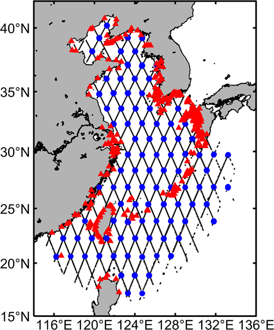
Figure 3 Locations of tidal gauge stations (red triangles) and cross points of altimeters (blue dots). The black solid lines show the altimeter tracks.

The correlation coefficien

$\begin{array}{ll}CC=[{\displaystyle \sum _{i=1}^n(X_m-\overline{X_m})(X_o-\overline{X_o})}]/{[{\displaystyle \sum _{i=1}^n{(X_m-\overline{X_m})}^2\sum _{i=1}^n{(X_o-\overline{X_o})}^2}]}^{1/2}& (1)\end{array}$

where n is the number of the variable values; X_m and $\overline{X_m}$ are time-varying model results and time-averaged values, respectively; X_o and $\overline{X_o}$ are time-varying values of observed results and time-averaged values, respectively.

(2) The root-mean-square discrepancy was used to evaluate both the amplitude and phase lag of the error in one metric (Wang et al., 2012; Blakely et al., 2022)

$\begin{array}{ll}DH=\sqrt{0.5\sum _k[{(A_o^k)}^2+{(A_m^k)}^2-2A_o^k{A}_m^{k}cos({\theta }_o^k-{\theta }_m^k)]}& (2)\end{array}$

$\begin{array}{ll}\overline{DH}=\frac{1}{N}\sum _{j=1}^{N}DH(j)& (3)\end{array}$

where A and θ are the amplitude and phase lag of the kth constituent, o denotes observed amplitude/phase lag, and m denotes simulated amplitude/phase lag.

(3) The relative bias

$\begin{array}{ll}RB=[{\displaystyle \sum _{i=1}^n{(X_m-X_o)}^2/}{\displaystyle \sum _{i=1}^n\left|X_o\right|}]\times 100\%& (4)\end{array}$

Figure 4 shows the comparisons between the simulated and observed amplitudes and phase lags of M₂, S₂, K₁, and O₁ tides from tidal gauge stations. The differences between simulated results and observations from tidal gauge stations are calculated and listed in Table 1. The correlation coefficients between the simulated amplitudes of M₂, S₂, K₁, and O₁ tides and observations from altimeter cross points in EXP 1-3 are larger than 0.92, 0.88, 0.88, and 0.91, respectively. The correlation coefficients between the simulated phase lags of M₂, S₂, K₁, and O₁ tides and observations from altimeter cross points in EXP 1-3 are larger than 0.89, 0.95, 0.95, and 0.85, respectively. For the amplitude, the relative bias of the M₂, S₂, K₁, and O₁ constituents between the observed and simulated harmonic constants in EXP 1-3 are smaller than 4.3%, 5.2%, 4.8%, and 4.9%, respectively. For the phase lag, the relative bias of M₂, S₂, K₁, and O₁ constituents in EXP 1-3 are smaller than 6.3%, 3.2%, 3.7%, and 6.2%, respectively. The $\overline{DH}$ between the simulated results and observations from satellite altimeters of M₂, S₂, K₁, and O₁ tides are (10.7, 15.7, 17.7, 17.4 cm) in EXP 1, (11.4, 15.7, 17.3, 18.0 cm) in EXP 2, and (10.5, 15.2, 17.2, 16.1 cm) in EXP 3. According to the calculations of the average absolute differences, correlation coefficients and root-mean-square discrepancies, the simulated results of EXP 3 fit the observations best, which has the smallest differences and highest correlation coefficient.

FIGURE 4

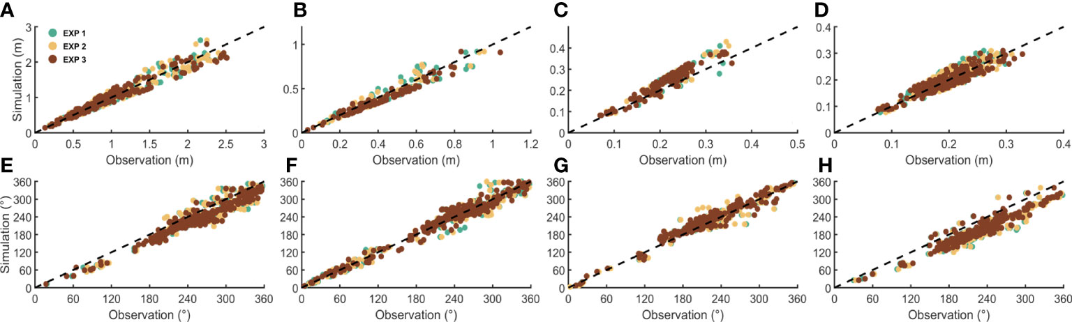
Figure 4 (A–D) Comparisons between the simulated and observed amplitudes of M₂, S₂, K₁, and O₁ tides from tidal gauge stations, respectively. Colors denote different BFC schemes. (E–H) Comparisons between the simulated and observed phase lags of M₂, S₂, K₁, and O₁ tides, respectively.

TABLE 1

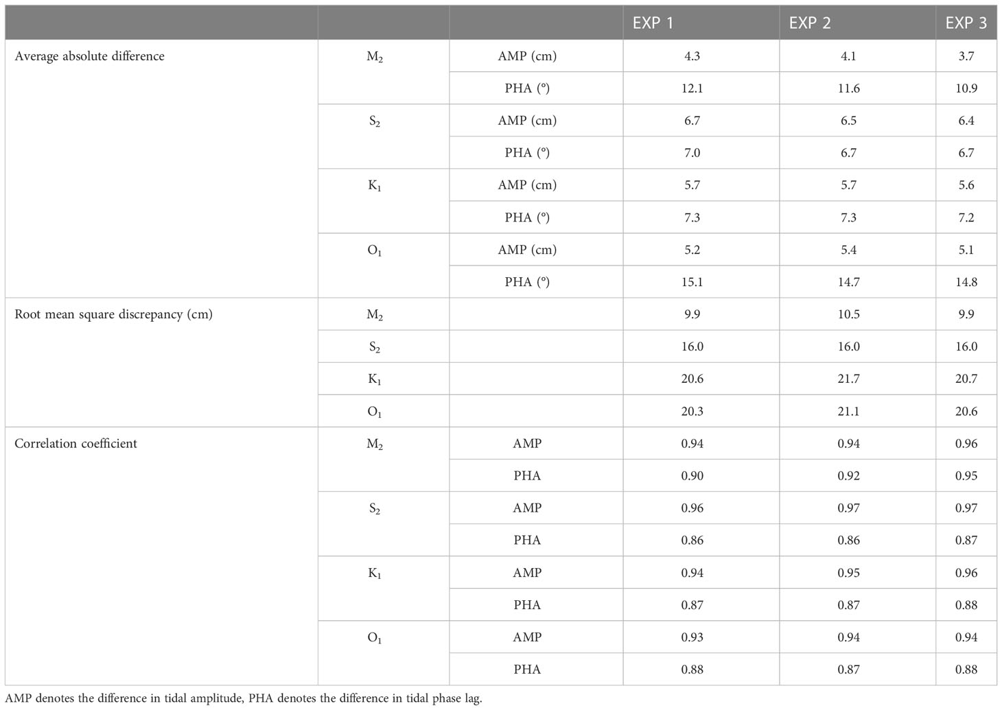
Table 1 The differences of tidal harmonic constants compared with observations from tidal gauge stations.

The tidal characteristics in the East China Seas are discussed based on the distributions of co-amplitude, co-phase, and tidal current ellipses of the four principal tidal constituents generated from the harmonic analysis of model results. As the simulated results from the SV-BFC scheme have the smallest root-mean-square discrepancy, the cotidal charts of M₂, S₂, K₁, and O₁ tides in EXP 3 are depicted in Figures 5A–D. The four principal tidal constituents amplified in the coastal regions under the effect of shoaling and narrowing, and the study area is significantly dominated by semidiurnal tides. The simulated results show that the tidal currents propagating from the Pacific Ocean into the East China Sea are affected by coastal topography, and tidal currents mainly propagate as rotating waves in a counterclockwise direction. The co-amplitude lines of the semidiurnal tides show that the largest amplitude, about 2 m for M₂ tide and 1 m for S₂ tide, exists in the West Korea Bay and the eastern coasts of Zhejiang and Fujian provinces (Figures 5A, B). For diurnal tides, the largest amplitude (about 0.3 m) exists in the Liaodong Bay, the West Korea Bay and the eastern coasts of Zhejiang and Fujian provinces (Figures 5C, D). The variations in the maximum tidal elevation between different BFC schemes are depicted in Figures 6A, B. The average values of the maximum tidal elevation of EXP 1 are 0.26 m, 0.32 m, 0.24 m, and 0.29 m less than those of EXP 3 in the West Korea Bay and eastern coasts of Jiangsu, Zhejiang and Fujian provinces, respectively. However, the maximum tidal elevation of EXP 1 around Jeju island is about 0.10 m larger than that in EXP 3. The average values of the maximum tidal elevation of EXP 2 are 0.14 m, 0.27 m, 0.24 m, and 0.35 m less than those of EXP 3 in the West Korea Bay and eastern coasts of Jiangsu, Zhejiang and Fujian provinces, respectively.

FIGURE 5

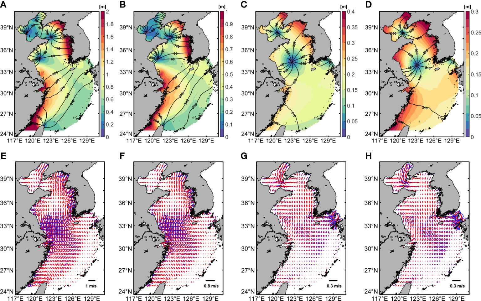
Figure 5 (A–D) Cotidal charts for M₂, S₂, K₁, and O₁ tides in EXP 3, respectively. Colormaps denote the magnitude of the co-amplitude (m). Contour lines are the co-phase lines (°). (E–H) Tidal current ellipses for M₂, S₂, K₁, and O₁ tides from the surface currents (blue) and bottom currents (red) in EXP 3, respectively.

FIGURE 6

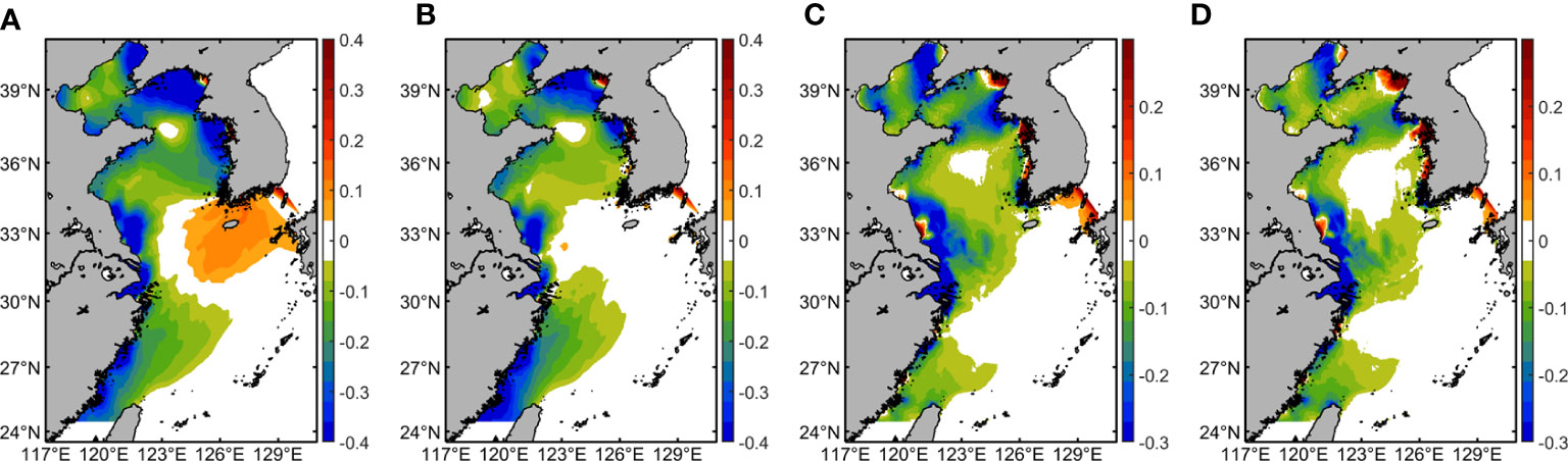
Figure 6 (A, B) Differences between the maximum tidal elevations (MTE) of EXP 1 and EXP 2 to those of EXP 3 (MTE_EXP1,2 - MTE_EXP3, unit: m). (C, D) Differences between the maximum bottom current velocity (MCV) of EXP 1 and EXP 2 to those of EXP 3 (MCV_EXP1,2 - MCV_EXP3, unit: m/s).

The co-phase lines show that there are four counterclockwise amphidromic systems for semidiurnal tides located in the Qinhuang Island, the Yellow River Estuary, the Chengshanjiao, and the Haizhou Bay, respectively, and two amphidromic systems for diurnal tides located in the Bohai Strait and middle of the South Yellow Sea (Figures 5A–D). The location of the amphidromic point is sensitive to the bottom friction, bottom topography, and coastlines (Fang et al., 1999). The locations of amphidromic points in this study coincide with previous studies (Fang et al., 2004; Zhu and Liu, 2012; Huang et al., 2017; Pringle et al., 2018). As the locations of the amphidromic points of M₂ and S₂ tides are almost similar, as well as the K₁ and O₁ tides, therefore only the comparisons of M₂ and K₁ tides are carried out. A comparison of the locations of the amphidromic points between different BFC schemes is depicted in Figure 7. The amphidromic systems of semidiurnal constituents in the Yellow River Estuary and Haizhou Bay are clustered. For the amphidromic points on the eastern coast of the Chengshanjiao, the amphidromic points of EXP 1 and EXP 2 are in the northwest of that from EXP 3, respectively. For diurnal constituents, the amphidromic points from different BFC schemes in the Bohai Strait are clustered. For those on the eastern coast of Jiangsu province, the amphidromic points of EXP 1 and EXP 2 are in the northwest of that from EXP 3.

FIGURE 7

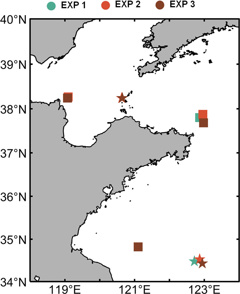
Figure 7 Locations of amphidromic points of M₂ tide (rectangles) and K₁ tide (pentagrams), respectively. Colors denote different experiments.

The tidal current ellipses of tidal currents on the surface layer and bottom layer of EXP 3 are depicted in Figures 5E–H. The tidal current ellipses show the velocity vector tracks for a certain constituent, in which the major axis and minor axis correspond to the maximum and minimum tidal velocity of this constituent, respectively. Due to the complex topography of coastal seas, such as fjords, islands, and tidal sand ridges, the ellipticity of the tidal ellipse in coastal regions is larger, while that in the outer sea is smaller. The results show that the amplitude of the tidal current velocity of semidiurnal constituents is larger than that of diurnal constituents. The strong tidal currents of semidiurnal constituents are found in the West Korea Bay, the eastern coast of Jiangsu province, and the Taiwan Strait, while the strong currents of diurnal constituents are mainly found in the Bohai Strait and the Liaodong Bay. The distributions of tidal ellipses for bottom currents are similar to the surface currents except for the decreasing amplitudes of tidal current velocity. The variations in the maximum bottom current velocity between different BFC schemes are shown in Figures 6C, D. The average values of the maximum bottom current velocity of EXP 1 are 0.08 m/s, 0.23 m/s, 0.14 m/s, and 0.08 m/s less than those of EXP 3 in the West Korea Bay, and the eastern coasts of Jiangsu, Zhejiang and Fujian provinces respectively, while the values of maximum bottom current velocity in EXP 2 are 0.03 m/s, 0.21 m/s, 0.10 m/s, and 0.11 m/s less than those of EXP 3.

3 Results

3.1 Tidal energy flux

To understand the tidal dynamics and to explain the mechanisms of the processes of four principal tidal constituents, the distribution of tidal energy in the East China Seas is investigated in this section. Following Garrett (1975) and Egbert and Ray (2000), the expression for the tidal energy flux P is:

$\begin{array}{ll}P=\rho g\langle U\zeta \rangle & (5)\end{array}$

where U is the volume transport vector, which equals velocity times water depth; ζ is sea surface elevation; the bracket 〈 〉 denotes time average. To improve the accuracy of the estimation, the final results are the average values of 15 tidal cycles of the four principal tidal constituents.

The vectors of tidal energy flux in the East China Seas of EXP 3 are shown in Figures 8A–D. For semidiurnal constituents (Figures 8A, B), the tidal energy flux in the northwestern Pacific Sea is westward and divided into two parts: one branch crosses the Ryukyu Islands into the East China Sea, and the other branch crosses the Luzon Strait into the South China Sea. The semidiurnal tide entering the East China Sea from the Tokara Strait can fold to the northwest and continue to spread forward with progressive waves. When arriving on the western coast of Kyushu, Japan, it is divided into two branches: the west branch is the main branch, which continues to the northwest through the southwest side of Jeju Island and enters the Yellow Sea. The tidal energy flux entering the Yellow Sea mainly moves northward along the western coast of the Korean Peninsula, while part of the energy bends westward in the north Yellow Sea and enters the Bohai Sea through the Bohai Strait. The rest part turns back by the Shandong Peninsula and propagates southward along the coasts, forming a counterclockwise semidiurnal tidal wave system. Most of the semidiurnal tidal energy entering the East China Sea from the Ryukyu Islands is diverted into the Taiwan Strait by a counterclockwise rotation around the northern Taiwan island. The vectors of tidal energy flux of M₂ and S₂ constituents are similar, but the magnitude of S₂ tide is approximately one-fifth of the M₂ tide. For the diurnal constituents (Figures 8C, D), tidal energy flux from the Pacific Ocean can be divided into two parts: a small part diverts northwest into the East China Sea through the Tokara Strait; the rest is blocked by the topographical trench (Ryukyu trench), and continues to spread southwest along the Okinawa Trough, and enters the South China Sea through the Luzon Strait. The variations in the propagation of the tidal energy flux between semidiurnal and diurnal constituents are concluded: most of the semidiurnal energy flux transports into the East China Sea through the Ryukyu Islands, while the diurnal energy flux is obstructed by the topographical trench and mainly propagates into the South China Sea through the Luzon Strait, which also indicates that the study area is dominated by the semidiurnal constituents.

FIGURE 8

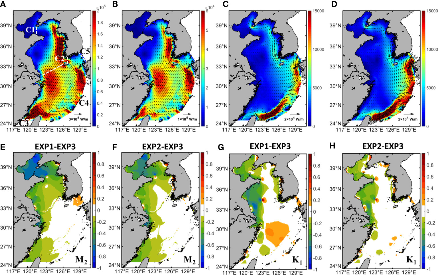
Figure 8 (A–D) Vectors of depth-averaged tidal energy flux for M₂, S₂, K₁, and O₁ tides in EXP 3, respectively. Colormaps denote the magnitude of tidal energy flux. (E–H) Relative differences of semidiurnal and diurnal tidal energy flux between EXP 1, EXP 2 to EXP 3, respectively.

The tidal energy flux of semidiurnal constituents is significantly larger than that of diurnal tides in the Yellow Sea and East China Sea, while the magnitudes of tidal energy flux of semidiurnal and diurnal tides through the eastern Taiwan Island to the northern Tokara Strait are similar. The existence of islands and topography variations have a great influence on the spatial distribution of tidal energy flux. The variations in tidal energy flux between different BFC schemes are shown in Figures 8E–H. The results show that the tidal energy flux transporting into the Bohai Sea and the Yellow Sea in the EXP 3 are larger than those in EXP 1 and EXP 2. Large differences in semidiurnal tidal energy flux appear in the West Korea Bay, and the eastern coasts of Jiangsu, Zhejiang and Fujian provinces. The semidiurnal tidal energy flux of EXP 1 is 62.7% smaller than that of EXP 3 in the Bohai Sea, while the semidiurnal tidal energy flux of EXP 2 is 47.9% smaller than that of EXP 3. The semidiurnal tidal energy flux in EXP 1 is (20.2%, 17.1%, 32.8%, 15.5%, 20.1%) smaller than those in EXP 3 in the West Korea Bay, South Yellow Sea, and eastern coasts of Jiangsu, Zhejiang and Fujian provinces, respectively. The semidiurnal tidal energy flux in EXP 2 is (9.6%, 13.7%, 26.9%, 12.8%, 25.1%) smaller than those in EXP 3 in the West Korea Bay, South Yellow Sea, and eastern coasts of Jiangsu, Zhejiang and Fujian provinces, respectively. On the other hand, the diurnal tidal energy flux is greatly weaker than that of semidiurnal components in the East China Seas, and the large variations in diurnal tidal energy flux between different BFC schemes mainly appear in the Bohai Sea and the eastern coasts of Shandong and Jiangsu provinces. The area-averaged values of tidal energy flux of diurnal constituents in EXP 1 are 26.9% and 47.1% less than those in EXP 3 in the Bohai Sea and the eastern coasts of Shandong and Jiangsu provinces, while the area-averaged values of diurnal tidal energy flux of EXP 2 are 16.5% and 29.8% less than those in EXP 3 in the Bohai Sea and the eastern coasts of Shandong and Jiangsu provinces. However, the average values of diurnal tidal energy flux in the northwestern Ryukyu Island of EXP 1 are 14.6% larger than those in EXP 3, while the average values of diurnal tidal energy flux in the northwestern Ryukyu Island of EXP 2 are only 5.8% larger than those in EXP 3.

To quantify the transport of tidal energy flux in the East China Seas, five sections are selected (C1-C5, Figure 8A). Tidal energy flux through section C1 means energy from the Yellow Sea entering the Bohai Sea, section C2 for the East China Sea entering the Yellow Sea, section C3 for the Taiwan Strait entering the East China Sea, section C4 (from the eastern Taiwan Island to the northern Tokara Strait) for the Pacific Ocean entering the East China Sea, and section C5 for the Korea Strait entering the East China Sea. The specific values of tidal energy flux of the M₂, S₂, K₁, and O₁ tides propagating through the five sections are listed in Table 2. The statistic values of tidal energy flux through C1-C5 are consistent with previous studies (Fang et al., 2004; Li et al., 2005; Zhu and Liu, 2012; Chen and Cheng, 2020). Moreover, the variations in tidal energy flux between different BFC schemes across five sections are studied. For diurnal constituents, the tidal energy flux of EXP 1 and EXP 2 through C1, C2, C3, and C4 is smaller than that in EXP 3, while the tidal energy flux of EXP 1 and EXP 2 through C5 is larger than that in EXP 3. The absolute differences in tidal energy flux between EXP 1 and EXP 2 to EXP 3 are less than 0.2 GW, while the relative differences are less than 7.1%. For semidiurnal constituents, the tidal energy flux of EXP 1 and EXP 2 through C1, C2, C3, and C4 is smaller than that in EXP 3, while the tidal energy flux of EXP 1 and EXP 2 through C5 is larger than that in EXP 3. The statistic values show that there are large variations in C1 and C3, and the relative differences are small in C2, C4, and C5. The semidiurnal tidal energy flux in EXP 1 through C1 and C3 are 66.7% and 29.1% smaller than those in EXP 3, while the semidiurnal tidal energy flux in EXP 2 through C1 and C3 is 51.5% and 33.8% smaller than those in EXP 3. On the other hand, the semidiurnal tidal energy flux in EXP 1 through C2 and C4 is 7.6% and 5.6% smaller than those in EXP 3, while the semidiurnal tidal energy flux in EXP 2 through C2 and C4 is 8.8% and 6.9% smaller than those in EXP 3. The statistical values show that the spatial distribution of BFCs in EXP 3 results in the increasing tidal energy flux transporting into the Bohai and the Yellow Sea, while the tidal energy from the Korea Strait decreases.

TABLE 2

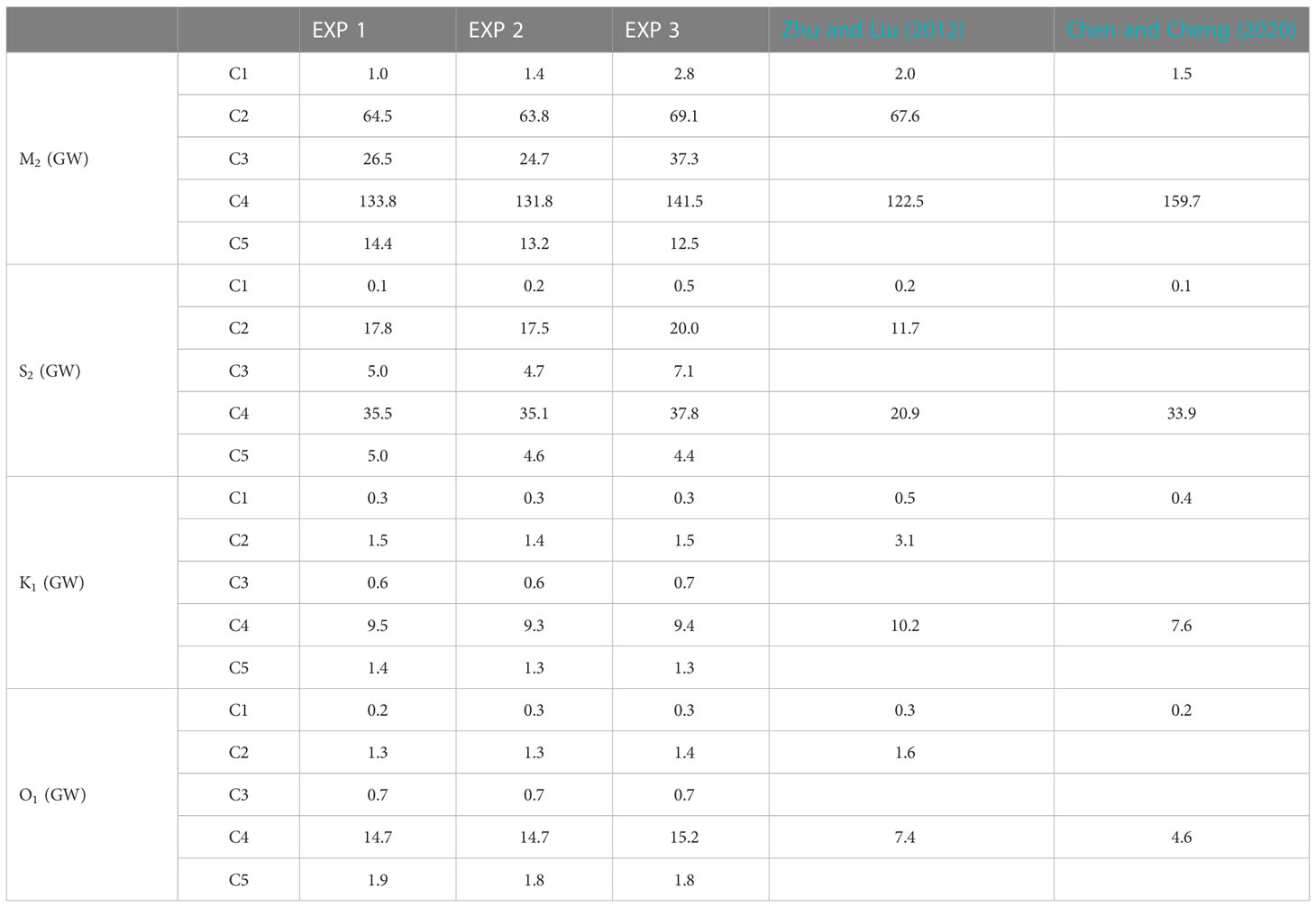
Table 2 Statistic values of tidal energy flux cross specific sections in East China Seas.

3.2 Bottom friction dissipation

According to the calculations of tidal energy flux through the specific sections, the total tidal dissipation of the Bohai, Yellow and East China Seas is listed in Table 3. The statistical values and the spatial distribution of total tidal dissipation locate in a reasonable range, which corresponds well with previous studies (Zhao et al., 1993; Li et al., 2005; Zhu and Liu, 2012; Zhu et al., 2014; Wu et al., 2018; Chen and Cheng, 2020). The results show that semidiurnal tides mainly dissipate in the Yellow Sea, while diurnal tides mainly dissipate in the East China Sea. The variations in total dissipation of semidiurnal constituents are significant, while those of diurnal constituents are neglectable. The semidiurnal tidal energy dissipated more in EXP 3 compared with EXP 1 and EXP 2, while the total dissipations of diurnal tides in EXP 1-3 have few differences. The total tidal dissipation of semidiurnal tides of EXP 1 and EXP 2 in the Bohai and Yellow Sea is less than that in EXP 3. However, the total dissipation of semidiurnal constituents of EXP 1 and EXP 2 is larger than that in EXP 3 in the East China Sea. On the other hand, the variations in total dissipation of diurnal constituents between different BFC schemes in the Yellow and East China Seas are neglectable, while the total dissipation of diurnal constituents in the Bohai Sea of EXP 1 is smaller than that in EXP 3.

TABLE 3

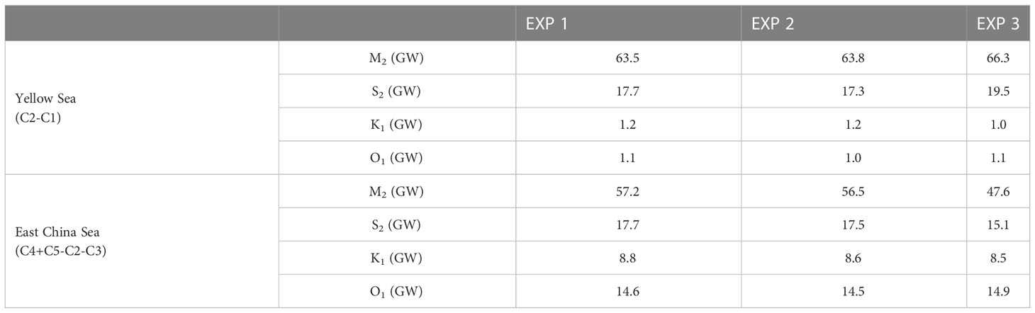
Table 3 The total tidal dissipation in the Yellow and East China Seas.

The tidal dissipation rate is estimated as a balance between the rate of working by tidal forces and the energy flux divergence (Egbert and Ray, 2000). The primary dissipation mechanisms for global tides are boundary layer dissipation and internal tide dissipation representing barotropic to baroclinic tidal conversion (Munk, 1997). For coastal areas, tidal dissipation is dominated by the bottom friction effect, and the expression for the bottom friction dissipation rate D is:

$\begin{array}{ll}D=\rho C_d\langle {\stackrel{\rightharpoonup }{u}}^3\rangle & (6)\end{array}$

where C_d is the bottom friction coefficient (BFC). The bottom friction dissipation of the four principal tidal constituents in EXP 3 is depicted in Figures 9A–D. The bottom friction dissipation of M₂ tide is near an order of magnitude larger than S₂ tide, and three orders of magnitude larger than diurnal constituents. The results show that large dissipation of semidiurnal constituents occurs in shallow areas with strong tidal currents, such as the West Korea Bay, eastern coasts of Jiangsu, Zhejiang and Fujian provinces. The bottom friction dissipation in the Okinawa Trough is three orders of magnitude less than that in the Yellow Sea. However, large dissipation of diurnal constituents occurs in the Bohai Strait, the Korea Strait, and the South Yellow Sea. According to equation (6), the estimation of bottom friction dissipation is closely related to the bottom friction coefficient and bottom current velocity cubed. The average values of semidiurnal and diurnal bottom friction dissipation in the Bohai Sea, Yellow Sea and East China Sea are listed in Table 4. The relative differences in bottom friction dissipation between different BFC schemes are depicted in Figures 9E–H. The results show that the variations in bottom friction dissipation are significantly related to the magnitude and spatial distribution of BFCs. The bottom friction dissipation significantly increases in the high-valued BFC areas. Large variations in tidal dissipation mainly appear in the shallow coastal areas and the South Yellow Sea (Figures 9E, F). The bottom friction dissipation of semidiurnal constituents in EXP 1 is 0.208 W/m² less than that in EXP 3 in the West Korea Bay, while that in EXP 2 is 0.203 W/m² less than EXP 3. For the coastal areas of Jiangsu and Fujian provinces, the bottom friction dissipation of semidiurnal tides in EXP 1 is 0.011 W/m² and 0.017 W/m² smaller than EXP 3, while those in EXP 2 are 0.011 and 0.019 W/m² smaller than EXP 3. The semidiurnal bottom friction dissipation in EXP 1 is 0.0078 W/m² larger than EXP 3 in the South Yellow Sea, while those in EXP 2 are 0.0082 smaller than EXP 3. On the other hand, the variations in diurnal tidal dissipation between different BFC schemes mainly appear in the Bohai Sea, the West Korea Bay, the middle of the South Yellow Sea, and the northwestern Ryukyu Island (Figures 9G, H). The average values of diurnal tidal dissipation in EXP 1 and EXP 2 are larger than those in EXP 3 in the Bohai Sea, the West Korea Bay, and the northwestern Okinawa Trough. The average value of diurnal tidal dissipation in EXP 1 is 17.9% larger than that in EXP 3 in the South Yellow Sea, while the average value of diurnal tidal dissipation in EXP 2 is 15.6% smaller than EXP 3.

FIGURE 9

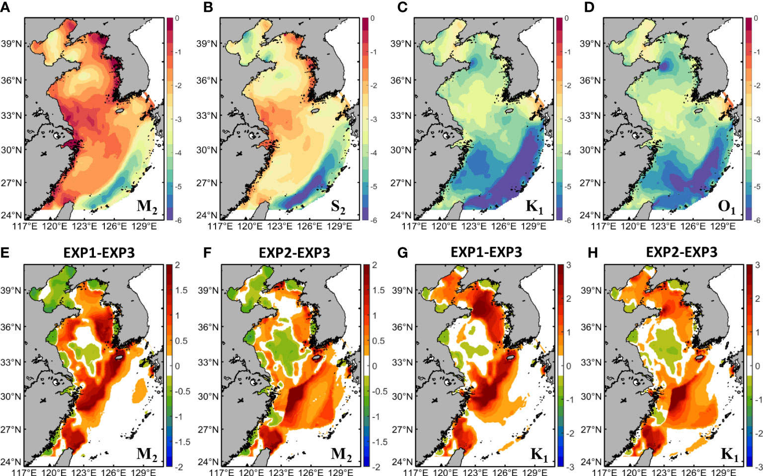
Figure 9 (A–D) Estimations of bottom friction dissipation for M₂, S₂, K₁, and O₁ tides in EXP 3 on a log scale, respectively (log₁₀D, unit: log₁₀(W/m²)). (E–H) Relative differences of semidiurnal and diurnal bottom friction dissipation between EXP 1, EXP 2 to EXP 3, respectively.

TABLE 4

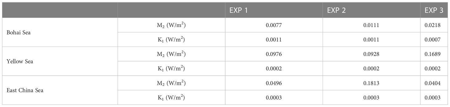
Table 4 The estimated bottom friction dissipation in the East China Seas.

The variations in bottom friction dissipation are closely related to the magnitude and spatial distribution of BFCs (Figures 9E–H). Signell and Geyer (1991) and Zhong and Li (2006) concluded that the headland-shaped coastal topography combined with strong tidal currents in shallow areas could result in turbulent eddies and therefore strengthened energy dissipation. The tidal sand ridges on the eastern coast of Jiangsu province impede the propagation of tidal currents and result in turbulent eddies and high tidal dissipation. On the other hand, the composition of seabed sediments can influence the magnitude of tidal dissipation as well. The SD-BFCs in the northwestern Ryukyu Island result in high bottom friction dissipation, while the sediment type of this area is sand, and the surrounding sediment environments are composed of clay, volcanic sand gravel, siliceous mud, and calcareous ooze (Dutkiewicz et al., 2015; Pringle et al., 2018). Large grain size and high suspended sediment concentration can also enlarge tidal dissipation, e.g. the eastern coast of Jiangsu province and Hangzhou Bay. The high-valued BFC areas in EXP 3 are closely related to water depth, sediment environment, and coastal topography (Qian et al., 2021), and therefore the bottom friction dissipation increases in the downstream sides of headland topography and those areas with mixed sediment types.

4 Discussions

4.1 Relations between BFC and tidal dynamics versus water depth

The regions that dissipate large amounts of energy are identified from the modelling results. The variations of tidal energy dissipation are greatly similar to the spatial distributions of BFCs, which denotes that the estimation of tidal energy dissipation is mainly influenced by the spatial distributions of BFCs. The specific areas performed with large variations in BFCs and strong tides are the West Korea Bay, the eastern coasts of Jiangsu, Zhejiang and Fujian provinces, and the middle of the South Yellow Sea. The average values of water depth in the West Korea Bay, the eastern coasts of Zhejiang and Fujian provinces, and the South Yellow Sea are 48.8, 34.2, and 51.2 m, respectively. For the West Korea Bay, the increasing BFCs and bottom current velocity relate to larger amounts of tidal dissipation. Based on the tidal propagation in the Yellow Sea, the coastal currents flow along the headland-shaped topography, which will enlarge form drag.

Although the averaged values of tidal dissipation of different BFC schemes in the eastern Jiangsu province are similar, the averaged values of the bottom current velocity of semidiurnal and diurnal tides are ~0.1 m/s and 0.01 m/s, respectively.

The variations in the spatial distributions of BFCs and velocity fields between different BFC schemes are depicted in Figures 2C, D and Figure 10, respectively. Significant variations in the magnitude and spatial distributions of BFCs between EXP 1 and EXP 3 appear in the coastal areas and middle of the South Yellow Sea, while those of EXP 2 in the northwestern Ryukyu Islands are larger than EXP 3 (Figures 2C, D). It can be seen that the variations in the bottom current velocity of semidiurnal and diurnal constituents are negatively related to the spatial distributions of BFCs. In EXP 3, the average BFC values in the West Korea Bay, the eastern coasts of Jiangsu and Fujian provinces are (0.02311, 0.00228, 0.00285), respectively, which are larger than those in EXP 1; however, the average BFC values in the eastern coast of Zhejiang province, the South Yellow Sea, and northwestern Ryukyu Islands are (0.00169, 0.00145, 0.00182), respectively, which are smaller than those in EXP 1. In EXP 2, the average BFC values in the West Korea Bay, the eastern coasts of Jiangsu, Zhejiang and Fujian provinces, and the South Yellow Sea are (0.00143, 0.00197, 0.00151, 0.00252, 0.00124), respectively, which are smaller than those in EXP 3; however, the average BFC value in the northwestern Ryukyu Islands is 0.01553, which are larger than those in EXP 3. Moreover, the variations in BFCs and velocity field of diurnal constituents are similar to semidiurnal constituents, but the values of variations in the velocity field are an order of magnitude less than those from semidiurnal constituents.

FIGURE 10

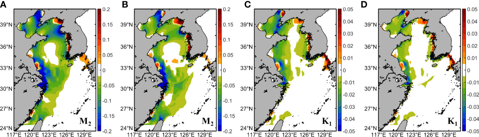
Figure 10 (A, B) Differences between the time-averaged semidiurnal bottom current velocity of EXP 1 and EXP 2 to those of EXP 3 (unit: m/s), respectively. (C, D) Differences between the time-averaged diurnal bottom current velocity of EXP 1 and EXP 2 to those of EXP 3 (unit: m/s), respectively.

Changes in the physical factors that control bottom friction dissipation undoubtedly play a role in these observed changes. Significant effects of bathymetry, bottom friction coefficients and ocean bedforms on tidal energy transport have been investigated (Blakely et al., 2022). The relationships between BFCs, bottom current velocity and bottom friction dissipation versus water depth in the whole East China Seas and those highlighting areas are depicted in Figure 11. The average values of the bottom current velocity of semidiurnal tides are an order of magnitude larger than those of diurnal tides, while the average values of bottom friction dissipation of semidiurnal tides are three orders of magnitude larger than those of diurnal tides. In the East China Seas, the bottom friction dissipation of semidiurnal constituents decreases versus the increasing water depth, while that of diurnal constituents has two peaks at 37 m and 97 m (Figure 11A). The average values of BFCs in EXP 2 and EXP 3 first decrease versus the increasing water depth, and then increase until becoming a constant, while the bottom current velocity of semidiurnal and diurnal tides both increase to peaks at 7.5 m and 32.5 m and then decrease. The first peak of diurnal tidal dissipation is proportional to the current velocity, and the second peak is inversely proportional to the current velocity. The variations in bottom friction dissipation of semidiurnal constituents between different BFC schemes are small, but the average values of diurnal tidal dissipation in 37 m of EXP 1 and EXP 2 are 66.7% larger than that in EXP 3. However, the variations in bottom friction dissipation of semidiurnal tides versus water depth in the coastal areas with high-values BFCs are different. For the West Korea Bay, the semidiurnal tidal dissipation first increases versus the increasing water depth and then decreases at 12 m (Figure 11B). The peak values of semidiurnal tidal dissipation in EXP 1 and EXP 2 are 22.0% and 11.6% smaller than EXP 3, while the corresponding values of semidiurnal current velocity in EXP 1 and EXP 2 are 5.0% and 12.6% smaller than EXP 3. At the same time, the average values of BFCs in EXP 2 and EXP 3 decrease when the water depth is less than 67.5 m. For the eastern coasts of Zhejiang and Fujian provinces, the maximum values of semidiurnal tidal dissipation of EXP 1 and EXP 2 are 0.1686 W/m² and 0.1707 W/m² in the water depth of around 135 m, while the maximum value of semidiurnal tidal dissipation of EXP 3 is 0.1512 W/m² in the water depth around 15 m (Figure 11C). The average values of BFCs in EXP 2 are in the interval of (0.0021, 0.0025), while those in EXP 3 decrease from 0.005 versus the increasing water depth. The corresponding semidiurnal current velocity reaches the maximum value at 135 m, and the maximum velocity of EXP 1 and EXP 2 is 17.6% and 21.1% smaller than EXP 3. On the other hand, the maximum values of diurnal tidal dissipation in EXP 1 and EXP 2 are 1.2×10^-4 W/m² and 1.4×10^-4 W/m² in the water depth of around 135 m, while that in EXP 3 is 0.7×10^-4 W/m² in the water depth around 55 m. Meanwhile, the maximum values of diurnal current velocity in EXP 1 and EXP 2 are 13.6% less than that in EXP 3 in the water depth of around 135 m. For the South Yellow Sea, the semidiurnal tidal dissipation decreases versus the increasing water depth, and then slightly increases when the water depth is larger than 75 m. The relationship between semidiurnal tidal dissipation and water depth is similar to the relationship between the semidiurnal current velocity and water depth. Although the average values of semidiurnal current velocity in EXP 1 and EXP 2 are 14.6% and 6.4% smaller than that in EXP 3, the average value of semidiurnal tidal dissipation in EXP 1 is 22.3% larger than EXP 3, while that in EXP 2 is 11.6% smaller than EXP 3. It can be seen that the variations in bottom friction dissipation are similar to the variations in the tidal current velocity, while the effects of BFCs become more important in the coastal shallow areas.

FIGURE 11

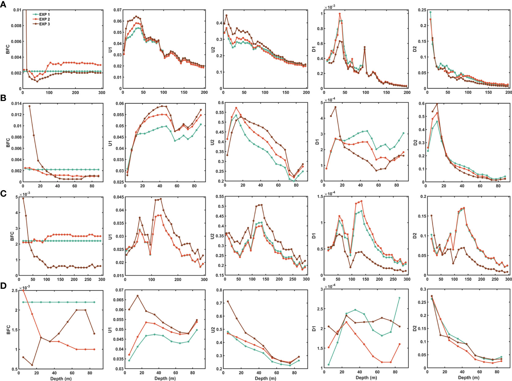
Figure 11 Relations of the BFCs, bottom current velocity of diurnal (U1) and semidiurnal (U2) tides, bottom friction dissipation of diurnal (D1) and semidiurnal (D2) tides versus water depth in the East China Seas (A row), the West Korea Bay (B row), the Zhejiang-Fujian provinces (C row), the middle South Yellow Sea (D row), respectively."

4.2 Influence on the parameter h/u³

Tidal mixing is essential in the coastal shallow areas, as it is one of the main mechanisms for the transport of nutrients to the euphotic zones, and also plays an important role in the water mass formation process and thermohaline circulation (Bray, 1988a; Lavin and Organista, 1988; Alvarez-Borrego and Lara-Lara, 1991; Argote et al., 1995). According to the simulated results above, the magnitude and spatial distribution of bottom friction dissipation are closely related to the spatial distribution of BFCs. Simpson and Hunter (1974) suggested a simple model examining the transition between stratified and unstratified regimes controlled by the level of tidal mixing from the observed position of the front. They assumed that, if the area and time of interest were limited, the locus of front could be defined simply by the parameter h/u³. h/u³ could be used as the parameter which controlled the formation of a front and used to predict the occurrence of stratification. In general, the Simpson-Hunter number (SH) is frequently presented in the form as:

$\begin{array}{ll}SH={\text{log}}_{10}(\frac{h}{\left|\overline{u^3}\right|})& (7)\end{array}$

where h is water depth, and u is the depth-averaged current velocity. Figure 12A shows the spatial distribution of SH numbers in EXP 3. Small values of SH numbers denote that mixed conditions prevail, while large values denote stratified conditions are predicted (Simpson and Hunter, 1974; Pingree and Griffiths, 1978; Argote et al., 1995). The average values of SH numbers in the whole study area, the Bohai Sea, the Yellow Sea, and the East China Sea are (3.98, 3.61, 3.02, 4.57) in EXP 1, (3.96, 3.44, 2.96, 4.59) in EXP 2, (3.83, 3.10, 2.85, 4.50) in EXP 3. Large values of SH numbers mainly appear in the Okinawa Trough, and the middle of the South Yellow Sea, while the coastal areas have small values of SH numbers. Figures 12B, C show the variations in the SH numbers between different BFC schemes. Large differences mainly distribute in the shallow water areas with strong tidal currents, i.e. the Bohai Sea, the West Korea Bay, the Hangzhou Bay, and the eastern coasts of Jiangsu and Fujian provinces. The average values of SH numbers in EXP 1 are (0.51, 0.14, 0.22, 0.13, 0.16, 0.39, 0.16) larger than those in EXP 3 in the Bohai Sea, the West Korea Bay, the eastern coasts of Jiangsu, Zhejiang and Fujian provinces, the Hangzhou Bay and the South Yellow Sea, respectively. The average values of SH numbers in EXP 2 are (0.34, 0.05, 0.20, 0.10, 0.21, 0.39, 0.11) larger than those in EXP 3 in the Bohai Sea, the West Korea Bay, the eastern coasts of Jiangsu, Zhejiang and Fujian provinces, the Hangzhou Bay and the South Yellow Sea, respectively. Comparing the cubed depth-averaged current velocity between different BFC schemes (Figures 12D–F), the spatial distributions of SH numbers are closely related to the cubed current velocity. The small valued SH numbers of EXP 3 in the coastal areas and the Bohai Sea may relate with weak stratification effects and strong oceanic mixing. It can be seen that the increasing BFCs in shallow coastal areas, especially in the Bohai Sea, the North Yellow Sea, and the eastern coasts of Jiangsu, Zhejiang and Fujian provinces, can enlarge the values of SH numbers. However, the values of SH numbers in the West Korea Bay and Jianghua Bay with high-valued BFCs are increased by the decreasing current velocity. Simpson and Pingree (1978) found that the partitioning of the seas into stratified and mixed regimes separated by frontal boundaries, while the strong stratification was associated with values of SH numbers larger than 3, and the complete vertical mixing with low values of SH numbers (<1.5). The SH number has been tested by field observations and the databases of temperature and salinity profiles which determined the positions of fronts in the shelf seas (Garrett et al., 1978; Lie, 1989; Glorioso and Flather, 1995; Kobayashi et al., 2006). Du et al. (2022) used a 10-year dataset of satellite-derived suspended sediment concentrations to identify the spatiotemporal variations in suspended sediment fronts on the inner shelf of the East China Seas. They found that the local high-value and low-value SH regions corresponded to the local low-value and high-value frontal probability regions, respectively. However, the critical values of SH numbers for frontal boundaries are varied in different regions. This may be attributable to changes in the main source of heat input, boundary-driven turbulence, and wind force (Simpson and Sharples, 2012).

FIGURE 12

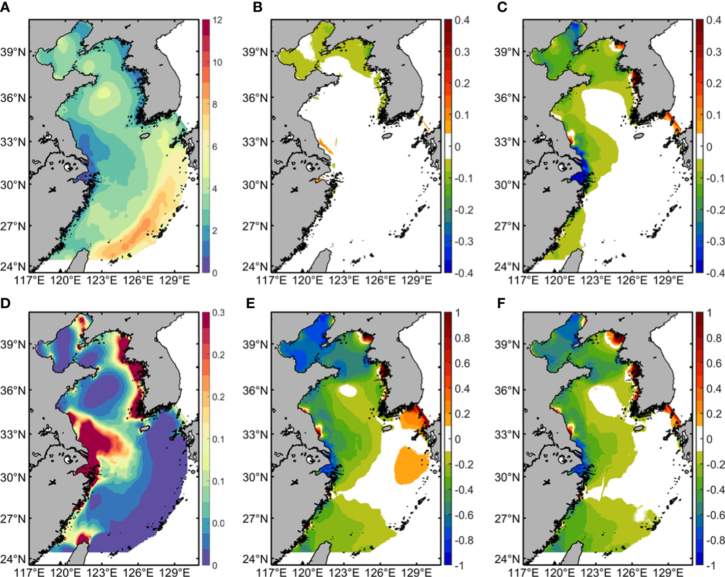
Figure 12 (A) Estimations of Simpson-Hunter (SH) number in EXP 3. (B, C) Relative differences of SH numbers between EXP 1, EXP 2 to EXP 3, respectively. (D) The cubed time-averaged and depth-averaged current velocity ($\overline{u^3}$) in EXP 3. (E, F) Relative differences of depth-averaged current velocity between EXP 1, EXP 2 to EXP 3, respectively.

5 Conclusions

To study the effects of spatial bottom friction parameterization schemes on tidal dynamics, a high-resolution model based on FVCOM was developed and used to simulate the four principal tidal constituents (M₂, S₂, K₁, O₁) in the East China Seas. The four principal tidal constituents in the East China Seas were simulated with different schemes of BFCs: the empirical constant (EC-BFC), sediment-dependent form (SD-BFC) and spatial distribution obtained from the adjoint tidal model with data assimilation (SV-BFC). The results were evaluated against the observations from satellite altimeters and tidal gauge stations, which demonstrated that the simulated results were reasonable and the simulated results obtained by the SV-BFC fitted observations best. The locations of amphidromic points calculated with EC-BFC and SD-BFC were in the northwest of those from SV-BFC.

The variations in tidal dynamics between different BFC schemes were closely related to the spatial distribution of BFC, especially in the high-valued BFC areas, e.g. the West Korea Bay, the South Yellow Sea, and the eastern coasts of Jiangsu, Zhejiang and Fujian provinces. The average value of the maximum tidal elevation with SV-BFC was approximately 0.26 m larger than those in the EC-BFC and SD-BFC schemes. Meanwhile, the average value of the maximum bottom current velocity with SV-BFC was approximately 0.12 m/s larger than those in the EC-BFC and SD-BFC. The SV-BFC scheme resulted in the increase of tidal energy flux transporting into the Bohai and Yellow Seas, while the tidal energy transporting from the Korea Strait was smaller than those from EC-BFC and SD-BFC. The variations in bottom friction dissipation were closely related to the spatial distribution of BFCs. The high-valued BFC areas of SV-BFC dissipated larger amounts of tidal energy, and the average values of SH numbers were lower than those in EC-BFC and SD-BFC. However, the values of SH numbers in the West Korea Bay and Jianghua Bay with high-valued BFCs were increased because of the decreasing current velocity under the headland-shaped topography. The SD-BFC in the northwestern Ryukyu Island resulted in high bottom friction dissipation, while the sediment type of this area was sand, and the surrounding sediment environments were composed of clay, volcanic sand gravel, siliceous mud, and calcareous ooze.

This study evaluates the effects of bottom friction parameterization schemes on the estimations of tidal energy flux, bottom friction dissipation, and oceanic mixing, and finds that the magnitude of tidal dissipation was closely related to water depth, bottom topography, and sediment types. This study mainly discusses the bottom friction dissipation, while the internal tide dissipation was also needed to be considered especially in deep-sea areas.

Data availability statement

The raw data supporting the conclusions of this article will be made available upon reasonable request and with authors’ permission. Requests to access the datasets should be directed to JZ, Jicai_Zhang@163.com.

Author contributions

SQ conducted the data analysis, software, model validation, writing, and visualization. YD and ZW conducted the formal analysis, software. JZ conceived the study, provided the methods and resources, and reviewed and edited the manuscript. JC, DW, and YW conducted the formal analysis and supervision. All authors contributed to the article and approved the submitted version.

Funding

This work was supported by the National Key Research and Development Plan of China (Grant No. 2022YFC2808304), the Science and Technology Commission of Shanghai Municipality (STCSM, Grant No. 21JC1402500), and the National Natural Science Foundation of China [Grant No. 41876086].

Acknowledgments

We thank Ms. Ling Tian for her help on the language improvement. We acknowledge all the reviewers for their valuable suggestions.

Conflict of interest

The authors declare that the research was conducted in the absence of any commercial or financial relationships that could be construed as a potential conflict of interest.

Publisher’s note

All claims expressed in this article are solely those of the authors and do not necessarily represent those of their affiliated organizations, or those of the publisher, the editors and the reviewers. Any product that may be evaluated in this article, or claim that may be made by its manufacturer, is not guaranteed or endorsed by the publisher.

References

Alvarez-Borrego S., Lara-Lara J. R. (1991). “The physical environment and primary productivity of the gulf of California, in the gulf and peninsular provinces of the californias,” in Mere. am. assoc. pet. geol, vol. 47 . Eds. Dauphin J. P., Simoneit B., (Tulsa, USA:American Association of Petroleum Geologists) 555–567.

Google Scholar

Argote M. L., Amador A., Lavin M. F. (1995). Tidal dissipation and stratification in the gulf of California. J. Geophys. Res. 100, 16103–16118. doi: 10.1029/95JC01500

CrossRef Full Text | Google Scholar

Blakely C. P., Ling G., Pringle W. J., Contreras M. T., Wirasaet D., Westerink J. J., et al. (2022). Dissipation and bathymetric sensitivities in an unstructured mesh global tidal model. J. Geophys. Res.: Oceans 127, e2021JC018178. doi: 10.1029/2021JC018178

CrossRef Full Text | Google Scholar

Bo T., Ralston D. K. (2020). Flow separation and increased drag coefficient in estuarine channels with curvature. J. Geophys. Res.: Oceans. 125, 1–25. doi: 10.1029/2020JC016267

CrossRef Full Text | Google Scholar

Bray N. A. (1988). Thermohaline circulation in the gulf of California. J. Geophys. Res. 93, 4993–5020. doi: 10.1029/JC093iC05p04993

CrossRef Full Text | Google Scholar

Brink K. H. (2016). Cross-shelf exchange. Annu. Rev. Mar. Sci. 8, 59–78. doi: 10.1146/annurev-marine-010814-015717

CrossRef Full Text | Google Scholar

Chen Y., Cheng P. (2020). Numerical modeling study of tidal energy and dissipation in the East China seas. J. Xiamen Univ. (Natural Science). 59 (1), 61–73.

Google Scholar

Cheng R. T., Ling C.-H., Gartner J. W., Wang P. F. (1999). Estimates of bottom roughness length and bottom shear stress in south San Francisco bay, California. J. Geophys. Res.: Oceans. 104, 7715–7728. doi: 10.1029/1998JC900126

CrossRef Full Text | Google Scholar

Chen C., Huang H., Beardsley R. C., Liu H., Xu Q., Cowles G. (2007). A finite volume numerical approach for coastal ocean circulation studies: comparisons with finite difference models. J. Geophys. Res.: Oceans. 112, 83–87. doi: 10.1029/2006JC003485

CrossRef Full Text | Google Scholar

Chen C., Liu H., Beardsley R. C. (2003). An unstructured grid, finite-volume, three-dimensional, primitive equations ocean model: application to coastal ocean and estuaries. J. Atmos. Ocean. Technol. 20 (1), 159–186. doi: 10.1175/1520-0426(2003)020<0159:AUGFVT>2.0.CO;2

CrossRef Full Text | Google Scholar

Chu D., Niu H., Wang Y. P., Cao A., Li L., Du Y., et al. (2021). Numerical study on tidal duration asymmetry and shallow-water tides within multiple islands: An example of the zhoushan archipelago. Estuar. Coast. Shelf Sci. 262, 107576. doi: 10.1016/j.ecss.2021.107576

CrossRef Full Text | Google Scholar

Chu D., Zhang J., Wu Y., Jiao X., Qian S. (2019). Sensitivities of modelling storm surge to bottom friction, wind drag coefficient, and meteorological product in the East China Sea. Estuar. Coast. Shelf Sci. 231, 106460. doi: 10.1016/j.ecss.2019.106460

CrossRef Full Text | Google Scholar

Cowen R. K., Sponaugle S. (2009). Larval dispersal and marine population connectivity. Annu. Rev. Mar. Sci. 1, 443–466. doi: 10.1146/annurev.marine.010908.163757

CrossRef Full Text | Google Scholar

Das S. K., Lardner R. W. (1991). On the estimation of parameters of hydraulic models by assimilation of periodic tidal data. J. Geophys. Res. 96, 187–196. doi: 10.1029/91JC01318

CrossRef Full Text | Google Scholar

Dutkiewicz A., Müller R. D., O’Callaghan S., Jónasson H. (2015). Census of seafloor sediments in the world’s ocean. Geology 43 (9), 795–798. doi: 10.1130/G36883.1

CrossRef Full Text | Google Scholar

Du Y., Zhang J., Wei Z., Yin W., Wu H., Yuan Y., et al. (2022). Spatio-temporal variability of suspended sediment fronts (SSFs) on the inner shelf of the East China Sea: The contribution of multiple factors. J. Geophys. Res.: Oceans 127, 1–25. doi: 10.1029/2021JC018392

CrossRef Full Text | Google Scholar

Dyer K. R., Soulsby R. L. (1988). Sand transport on the continental shelf. Annu. Rev. Fluid Mech. 20, 295–324. doi: 10.1146/annurev.fl.20.010188.001455

CrossRef Full Text | Google Scholar

Egbert G. D., Erofeeva S. Y. (2002). Efficient inverse modeling of barotropic ocean tides. J. Atmosp. Ocean. Technol. 19 (2), 183–204. doi: 10.1175/1520-0426(2002)0192.0.CO;2

CrossRef Full Text | Google Scholar

Egbert G., Ray R. (2000). Significant dissipation of tidal energy in the deep ocean inferred from satellite altimeter data. Nature 405, 775–778. doi: 10.1038/35015531

PubMed Abstract | CrossRef Full Text | Google Scholar

Egbert G. D., Ray R. D., Bills B. G. (2004). Numerical modeling of the global semidiurnal tide in the present day and in the last glacial maximum. J. Geophys. Res. C: Oceans 109 (3), 1–5. doi: 10.1029/2003JC001973

CrossRef Full Text | Google Scholar

Fang G., Kwok Y. K., Yu K., Zhu Y. (1999). Numerical simulation of principal tidal constituents in the south China Sea, gulf of tonkin and gulf of Thailand. Continent. Shelf Res. 19, 845–869. doi: 10.1016/S0278-4343(99)00002-3

CrossRef Full Text | Google Scholar

Fang G., Wang Y., Wei Z., Choi B. H., Wang X., Wang J. (2004). Empirical cotidal charts of the bohai, yellow, and East China seas from 10 years of TOPEX/Poseidon altimetry. J. Geophys. Res. 109 (C11), 1–13. doi: 10.1029/2004jc002484

CrossRef Full Text | Google Scholar

Fan R., Zhao L., Lu Y., Nie H., Wei H. (2019). Impacts of currents and waves on bottom drag coefficient in the East China shelf seas. J. Geophys. Res.: Oceans. 124, 7344–7354. doi: 10.1029/2019JC015097

CrossRef Full Text | Google Scholar

Gao X., Wei Z., Lv X., Wang Y., Fang G. (2015). Numerical study of tidal dynamics in the south China Sea with adjoint method. Ocean Model. 92, 101–114. doi: 10.1016/j.ocemod.2015.05.010

CrossRef Full Text | Google Scholar

Garrett C. (1975). Tides in gulfs. Deep Sea Res. Oceanogr. Abstr. 22 (1), 23–35. doi: 10.1016/0011-7471(75)90015-7

CrossRef Full Text | Google Scholar

Garrett C., Keeley J. R., Greenberg D. A. (1978). Tidal mixing versus thermal stratification in the gulf of Maine. Atmos Oceans. 16 (4), 403–423. doi: 10.1080/07055900.1978.9649046

CrossRef Full Text | Google Scholar

Glorioso P. D., Flather R. A. (1995). A barotropic model of the currents off SE south America. J. Geophys. Res. 100 (C7), 13427–13440. doi: 10.1029/95JC00942

CrossRef Full Text | Google Scholar

Guo X., Yanagi T. (1998). Three-dimensional structure of tidal current in the East China Sea and the yellow Sea. J. Oceanogr. 54, 651–668. doi: 10.1007/BF02823285

CrossRef Full Text | Google Scholar

Huang X., Zhang R., Ma Q., Jiang B., Sun J. (2017). Numerical simulation of tidal waves in bohai Sea and yellow Sea based on FVCOM. J. Dalian Ocean Univ. 32 (5), 617–624.

Google Scholar

Huettel M., Berg P., Kostka J. E. (2014). Benthic exchange and biogeochemical cycling in permeable sediments. Annu. Rev. Mar. Sci. 6, 23–51. doi: 10.1146/annurev-marine-051413-012706

CrossRef Full Text | Google Scholar

Jeffreys H. (1921). “Tidal friction in shallow seas,” in Philosophical transactions of the royal society of London. Series a, containing papers of a mathematical or physical character. 221, 239–264.

Google Scholar

Kang S. K., Lee S., Lie H. (1998). Fine grid tidal modeling of the yellow and East China seas. Continent. Shelf Res. 18 (7), 739–772. doi: 10.1016/S0278-4343(98)00014-4

CrossRef Full Text | Google Scholar

Kobayashi S., Simpson J. H., Fujiwara T., Horsburgh K. J. (2006). Tidal stirring and its impact on water column stability and property distributions in a semi-enclosed shelf sea (Seto inland Sea, Japan). Continent. Shelf Res. 26 (11), 1295–1306. doi: 10.1016/j.csr.2006.04.006

CrossRef Full Text | Google Scholar

Lavin M. F., Organista S. (1988). Surface heat flux in the northern gulf of California. J. Geophys. Res. 93, 14033–14038. doi: 10.1029/JC093iC11p14033

CrossRef Full Text | Google Scholar

Lee J. C., Jung K. T. (1999). Application of eddy viscosity closure models for the M₂ tide and tidal currents in the yellow Sea and the East China Sea. Continent. Shelf Res. 19 (4), 445–475. doi: 10.1016/S0278-4343(98)00087-9

CrossRef Full Text | Google Scholar

Lie H. J. (1989). Tidal fronts in the south-eastern hwanghae (Yellow Sea). Continent. Shelf Res. 9 (6), 527–546. doi: 10.1016/0278-4343(89)90019-8

CrossRef Full Text | Google Scholar

Li L., Guan W., Hu J., Cheng P., Wang X. H. (2018). Responses of water environment to tidal flat reduction in xiangshan bay: Part I hydrodynamics. Estuar. Coast. Shelf Sci. 206, 14–26. doi: 10.1016/j.ecss.2017.11.003

CrossRef Full Text | Google Scholar

Li P., Li L., Zuo J., Chen M., Zhao W. (2005). Tidal energy fluxes and dissipation in the bohai Sea, the yellow Sea and the East China Sea. Period. Ocean Univ. China 35 (5), 713–718.

Google Scholar

Lu X., Zhang J. (2006). Numerical study on spatially varying bottom friction coefficient of a 2D tidal model with adjoint method. Continent. Shelf Res. 26, 1905–1923. doi: 10.1016/j.csr.2006.06.007

CrossRef Full Text | Google Scholar

McWilliams J. C. (2006). Fundamentals of geophysical fluid dynamics (New York: Cambridge Univ. Press).

Google Scholar

Mellor G. L., Yamada T. (1982). Development of a turbulence closure model for geophysical fluid problems. Rev. Geophys. 20 (4), 851–875. doi: 10.1029/RG020i004p00851

CrossRef Full Text | Google Scholar

Mofjeld H. O. (1988). Depth dependence of bottom stress and quadratic drag coefficient for barotropic pressure-driven currents. J. Phys. Oceanogr. 18, 1658–1669. doi: 10.1175/1520-0485(1988)018<1658:DDOBSA>2.0.CO;2

CrossRef Full Text | Google Scholar

Munk W. (1997). Once again: Once again–tidal friction. Prog. Oceanogr. 40 (1), 7–35. doi: 10.1016/S0079-6611(97)00021-9

CrossRef Full Text | Google Scholar

Munk W., Wunsch C. (1998). Abyssal recipes II: energetics of tidal and wind mixing. Deep Sea Res. Part I: Oceanogr. Res. Pap 45, 1977–2010. doi: 10.1016/S0967-0637(98)00070-3

CrossRef Full Text | Google Scholar

Pawlowicz R., Beardsley B., Lentz S. (2002). Classical tidal harmonic analysis including error estimates in MATLAB using T_TIDE. Comput. Geosci. 28 (8), 929–937. doi: 10.1016/S0098-3004(02)00013-4

CrossRef Full Text | Google Scholar

Pingree R. D., Griffiths D. K. (1978). Tidal fronts on the shelf seas around the British isles. J. Geophys. Res.: Oceans 83 (C9), 1–8. doi: 10.1029/JC083iC09p04615

CrossRef Full Text | Google Scholar

Pringle W. J., Wirasaet D., Suhardjo A., Meixner J., Westerink J. J., Kennedy A. B., et al. (2018). Finite-element barotropic model for the Indian and Western pacific oceans: Tidal model-data comparisons and sensitivities. Ocean Model. 129, 13–38. doi: 10.1016/j.ocemod.2018.07.003

CrossRef Full Text | Google Scholar

Qian S., Wang D., Zhang J., Li C. (2021). Adjoint estimation and interpretation of spatially varying bottom friction coefficients of the M₂ tide for a tidal model in the bohai, yellow and East China seas with multi-mission satellite observations. Ocean Model. 161, 101783. doi: 10.1016/j.ocemod.2021.101783

CrossRef Full Text | Google Scholar

Signell R., Geyer W. (1991). Transient eddy formation around headlands. J. Geophys. Res.: Oceans 96 (C2), 2561–2575. doi: 10.1029/90JC02029

CrossRef Full Text | Google Scholar

Simpson J. H., Hunter J. R. (1974). Fronts in the Irish Sea. Nature 250 (5465), 404–406. doi: 10.1038/250404a0

CrossRef Full Text | Google Scholar

Simpson J. H., Pingree R. D. (1978). “Shallow sea fronts produced by tidal stirring,” in Oceanic fronts in coastal processes. Eds. Bowman M. J., Esaias W. E. (New York: Springer-Verlag), 29–42.

Google Scholar

Simpson J. H., Sharples J. (2012). Introduction to the physical and biological oceanography of shelf seas (New York: Cambridge University Press), 466.

Google Scholar

Taylor G. I. (1920). “I. tidal friction in the Irish Sea,” in Philosophical transactions of the royal society of London. Series a, containing papers of a mathematical orphysical character. 220, 1–33. doi: 10.1098/rsta.1920.0001

CrossRef Full Text | Google Scholar

Trowbridge J. H., Lentz S. J. (2018). The bottom boundary layer. Annu. Rev. Mar. Sci. 10, 397–420. doi: 10.1146/annurev-marine-121916-063351

CrossRef Full Text | Google Scholar

Wang X., Chao Y., Shum C., Yi Y., Fok H. S. (2012). Comparison of two methods to assess ocean tide models. J. Atmosp. Ocean. Technol. 29 (8), 1159–1167. doi: 10.1175/JTECH-D-11-00166.1

CrossRef Full Text | Google Scholar

Wang D., Liu Q., Lv X. (2014). A study on bottom friction coefficient in the bohai, yellow, and East China Sea. Math. Problems Eng. 2014, 1–7. doi: 10.1155/2014/432529

CrossRef Full Text | Google Scholar

Wang D., Zhang J., Wang Y. P. (2021). Estimation of bottom friction coefficient in multi-constituents tidal models using the adjoint method: temporal variations and spatial distributions. J. Geophys. Res.: Oceans 126, 1–20. doi: 10.1029/2020JC016949.

CrossRef Full Text | Google Scholar

Wu R., Jiang Z., Li C. (2018). Revisiting the tidal dynamics in the complex zhoushan archipelago waters: a numerical experiment. Ocean Model. 132, 139–156. doi: 10.1016/j.ocemod.2018.10.001

CrossRef Full Text | Google Scholar

Zhang X., Chu D., Zhang J. (2021). Effects of nonlinear terms and topography in a storm surge model along the southeastern coast of China: a case study of typhoon chan−hom. Natural Hazards. 107, 551–574. doi: 10.1007/s11069-021-04595-y

CrossRef Full Text | Google Scholar

Zhang J., Lu X., Wang P., Wang Y. P. (2011). Study on linear and nonlinear bottom friction parameterizations for regional tidal models using data assimilation. Continent. Shelf Res. 31, 555–573. doi: 10.1016/j.csr.2010.12.011

CrossRef Full Text | Google Scholar

Zhao B., Fang G., Cao D. (1993). Numerical modeling on the tides and tidal currents in the eastern China seas. Yellow Sea Res. 5, 41–61.

Google Scholar

Zhong L., Li M. (2006). Tidal energy fluxes and dissipation in the Chesapeake bay. Continent. Shelf Res. 26 (6), 752–770. doi: 10.1016/j.csr.2006.02.006

CrossRef Full Text | Google Scholar

Zhu X., Liu G. (2012). Numerical study on the tidal currents, tidal energy fluxes and dissipation in the China seas. Oceanol. ET Limnol. Sinica. 43 (3), 669–677.

Google Scholar

Zhu X., Song D., Bao X., Liu G. (2014). Tidal energy flux and dissipation in the Northwest pacific. J. Trop. Oceanogr. 33 (1), 1–9.

Google Scholar