
94% of researchers rate our articles as excellent or good
Learn more about the work of our research integrity team to safeguard the quality of each article we publish.
Find out more
ORIGINAL RESEARCH article
Front. Mar. Sci., 28 March 2023
Sec. Global Change and the Future Ocean
Volume 10 - 2023 | https://doi.org/10.3389/fmars.2023.1082170
 Susan Kay1*
 Arlene L. Avillanosa2
 Victoria V. Cheung3
 Hung N. Dao4
 Benjamin Jareta Gonzales5,6
 Herminie P. Palla2
 Radisti A. Praptiwi7,8
 Ana M. Queirós1
 Sévrine F. Sailley1
 Joel D. C. Sumeldan2
 Wan Mohd Syazwan9,10
 Amy Yee-Hui Then10
 Hin Boo Wee11
The seas of Southeast Asia are home to some of the world’s most diverse ecosystems and resources that support the livelihoods of millions of people. Climate change will bring temperature changes, acidification and other environmental change, with uncertain consequences for human and natural systems, but there has been little regional-scale climate modelling of the marine ecosystem. We present initial dynamically downscaled projections using a biogeochemical model suitable for coastal and shelf seas. A coupled physical-biogeochemical model with a resolution of 0.1° (approximately 11 km) was used to create projections of future environmental conditions under moderate (RCP4.5) and high (RCP8.5) greenhouse gas scenarios. Changes for different parts of the region are presented, including four sensitive coastal sites of key importance for biodiversity and sustainable development: UNESCO Biosphere Reserves at Cu Lao Cham-Hoi An in Vietnam, Palawan in the Philippines and Taka Bonerate-Kepulauan Selayar in Indonesia, and coastal waters of Sabah, Malaysia, which include several marine parks. The projections show a sea that is warming by 1.1 to 2.9°C through the 21st century, with dissolved oxygen decreasing by 5 to 13 mmol m-3 and changes in many other environmental variables. The changes reach all parts of the water column and many places are projected to experience conditions well outside the range seen at the start of the century. The resulting damage to coral reefs and altered species distribution would have consequences for biodiversity, the livelihoods of small-scale fishers and the food security of coastal communities. Further work using a range of global models and regional models with different biogeochemical components is needed to provide confidence levels, and we suggest some ways forward. Projections of this type serve as a key tool for communities and policymakers as they plan how they will adapt to the challenge of climate change.
The world’s oceans are warming, acidifying and deoxygenating, leading to shifts in the geographical range of many marine species, and these changes are expected to accelerate this century (IPCC, 2019; IPCC, 2021). Southeast Asia is particularly vulnerable to the effects of marine climate change: large populations live in coastal areas (Neumann et al., 2015) and rely heavily on marine resources and marine ecosystem services (Barange et al., 2014). In some Southeast Asian countries the ocean economy can account for 15 to 20% of total GDP (Ebarvia, 2016). In addition, the seas of this region host many sites of high ecological value such as the Coral Triangle linking the Philippines, Malaysia and Indonesia (Veron et al., 2011; Burke et al., 2012). The impact of climate change on the Southeast Asian marine environment is therefore of major social, economic and ecological concern, particularly its effects on fisheries and coral reefs.
Climate change is expected to impact the productivity of marine fisheries through changes in temperature, acidification, deoxygenation, the effects of sea level rise and other factors, and it is in the tropics that these changes are likely to first exceed natural variability (Lam et al., 2020). Small-scale fishers, who provide approximately half the fish for human consumption in Southeast Asia (Teh and Pauly, 2018), are particularly vulnerable to the effects of climate change (Barange et al., 2018). The aquaculture sector is similarly at risk, with potential economic and health consequences: cultivation of seaweed, caged fish and shellfish are important for the marine economy, food security, human nutrition, sustainable livelihoods and poverty alleviation in Southeast Asia (FAO, 2018; Monnier et al., 2020).
Climate change also poses a risk to coral reefs, which are areas of particularly high biodiversity: 76% of all coral species and 37% of coral reef fish species are found in the Coral Triangle (Burke et al., 2012). Rising temperatures and ocean acidification pose threats to coral reefs worldwide (Hoegh-Guldberg et al., 2007; Lough et al., 2018). Increasingly frequent and more extreme heat-waves cause damage to reefs through mass coral bleaching reducing long-term sustainability (Hughes et al., 2018). In addition, ocean acidification is altering ocean carbonate chemistry, limiting coral growth and degrading the physical structure of reefs (Burke et al., 2012; Lam et al., 2020). Coral reef degradation in Southeast Asia threatens the associated food web, jeopardizing dependent biodiversity and fisheries, and impacting regional food security, coastal protection and tourism, potentially costing the region billions of dollars in lost revenue (Burke et al., 2002; Cesar et al., 2003; Burke et al., 2012).
Given the potential impact of climate change on key marine ecosystems in Southeast Asia and coastal communities that depend upon them, adequately projecting the effects of climate change on Southeast Asian seas is a crucial step towards informing strategies for poverty alleviation and food security, UN Sustainable Development Goals 1 and 2 (https://sdgs.un.org/goals). Global climate models provide a broad picture of the environmental change that may be experienced in the region (IPCC, 2019; IPCC, 2021), however they have a coarse resolution and the biogeochemical models used are typically designed for open ocean conditions: they do not include the range of plankton functional types and nutrient interactions needed to accurately model more complex coastal ecosystems (Stock et al., 2011; Drenkard et al., 2021).
We present regional, dynamically downscaled projections of change in the physical environment and lower trophic level ecosystem of Southeast Asian seas, to the end of the 21st century (Kay, 2021). This work was undertaken in the context of a research project focused on building capacity in marine planning and sustainable use of marine resources in Southeast Asia (GCRF Blue Communities, https://www.blue-communities.org/). The project centered on four coastal sites which aim to support both coastal human populations and high biodiversity: UNESCO Biosphere Reserves at Cu Lao Cham-Hoi An in Vietnam, Palawan in the Philippines and Taka Bonerate-Kepulauan Selayar in Indonesia, and coastal waters of Sabah, Malaysia, which include several marine parks (Figure 1). Sustainable development of sites like these, and the wider region, requires an understanding of how the marine environment and its resources are likely to alter under future climate change. Information from global models may be unreliable, given the coastal location of the sites, but regional projections for Southeast Asian seas have not previously been available. We were also interested in the changing marine food resource across Southeast Asia, which requires an understanding of change in primary productivity at the base of the food chain. However global models give widely varying projections (see section 3.2.2) and regional models can give new insights; for example, studies of the Northwest European Shelf (Holt et al., 2016) have found that a regional model showed a different direction of change in net primary productivity for near-shore areas, compared to the global model it was based on. We therefore felt it was important to explore the potential for regional modelling of the area.
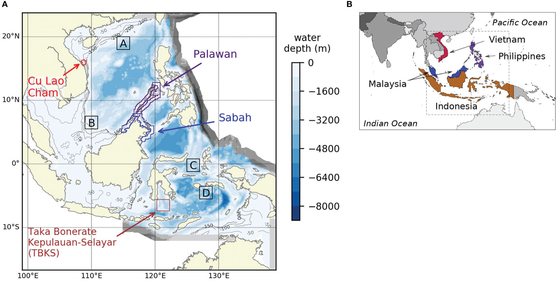
Figure 1 (A) shows the model domain and sample areas referred to in the text. Blue and grey areas are the model domain, with the colors showing water depth; the grey parts are near the open boundary and omitted from analysis in the rest of this paper. White shows sea areas outside the model domain. The four areas outlined and labelled in color show regions around the four coastal study sites. Boxes A, B, C and D are sample areas for four different offshore parts of the domain; their locations are given in section 2.2. (B) shows the modelled area embedded in the wider geographical context. The countries where the four coastal study sites are located are shown in color.
Our projections were created using a model with spatial resolution 0.1° (approximately 11 km) and a well-established biogeochemical/ecosystem model suited to coastal and shelf sea environments: the European Regional Seas Ecosystem Model (ERSEM; Blackford et al., 2004; Butenschön et al., 2016). This modelling system has previously been applied to coastal regions in many parts of the world, including Southeast Asia (Holt et al., 2009; Barange et al., 2014). The model was driven by outputs from a global climate model drawn from the Coupled Model Intercomparison Project Phase 5 (CMIP5; Taylor et al., 2011). We selected two Representative Concentration Pathways (RCPs) of greenhouse gases in the atmosphere (van Vuuren et al., 2011) to show a range of climate response: the moderate RCP4.5 scenario, under which atmospheric carbon dioxide concentration rises until mid-century and then stabilizes, and the more extreme RCP8.5 scenario, under which the concentration rises throughout the 21st century. The CMIP5 models are now being superseded by the more advanced CMIP6 set and the RCPs by Shared Socio-economic Pathways (SSPs), but it will be some time before regionally-downscaled versions of these models become available. In the meantime, this work offers a first look at what regional scale modelling offers for understanding climate change in Southeast Asian seas and makes recommendations for future downscaling efforts. The next section describes the modelling system and data used; section 3 presents the model outputs; section 4 discusses the implications of the projected change for people and ecosystems and the need for further modelling of this region.
The projections were created using the Proudman Oceanographic Laboratory Coastal Ocean Modelling System (POLCOMS; Holt and James, 2001) coupled to the European Regional Seas Ecosystem Model (ERSEM; Butenschön et al., 2016). Together, these simulate the movement of water, energy and dissolved and suspended material through the sea and the cycling of nutrients and carbon through the marine ecosystem.
POLCOMS is a three-dimensional model of physical processes, suitable for modelling both deep and shallow water and areas with steep bathymetry. It is a free surface baroclinic model, with varying water depth, and includes the effects of tides but not waves. Forty depth levels were used at each point, regardless of total water depth, distributed more closely in the upper parts of the water column than at depth (a modified sigma system). The minimum water depth was 10 m. When run at the 0.1° resolution used here, POLCOMS is able to explicitly model processes of riverine freshwater inputs, tidal mixing and coastal upwelling that are parameterized in CMIP5 global models (Holt et al., 2009; Drenkard et al., 2021). These processes can influence circulation patterns and nutrient distributions in near-shore waters, with potential effects on water temperature and productivity which could affect resources such as corals, aquaculture sites and production at higher trophic levels. Given the widely varying water depths and very steep shelf edges within the region (Figure 1) it is important to use a model with adequate vertical resolution – large parts of the shelf area are less than 100 m deep.
ERSEM models the transfer of carbon, nitrogen, phosphorus and silicate through the lower trophic levels of the marine ecosystem (Butenschön et al., 2016). It is one of the more complex models of its type and is well suited to modelling coastal and shelf-sea environments. It has four phytoplankton functional types, three zooplankton types and bacteria, as well as six categories of dissolved and particulate organic matter. The carbonate system is included, enabling changes in pH to be modelled. The stoichiometry is fully flexible: transfers of carbon, nitrogen, phosphorus and silicate are tracked separately, with no fixed ratios, and the chlorophyll to carbon ratio varies depending on levels of light and nutrients. Kearney et al. (2021), reviewing the features of biogeochemical components in the next generation of global models, CMIP6, note that variable stoichiometry and inclusion of larger phytoplankton groups can improve the simulation of trophic transfers, while resolution of multiple detritus types enables fuller representation of nutrient circulation in complex, shallow-water environments. In this work, interactions at the seabed were represented by a simple remineralization scheme, where organic matter falling to the seabed is adsorbed and inorganic nutrients and carbon are returned to the water column at a rate proportional to their benthic concentration.
ERSEM was coupled online to POLCOMS, with the ecosystem model running in each model cell at each timestep. The model configuration and Southeast Asia domain are part of the Global Coastal Modelling System (Holt et al., 2009), which has previously been applied to investigate the effect of climate change on fisheries and marine food resources in many parts of the world (Blanchard et al., 2012; Barange et al., 2014; Fernandes et al., 2016).
The model domain covered the region from 99.1 to 139.0°E and 16.7°S to 23.9°N at a resolution of 0.1° latitude and longitude, with all sea areas within 200 km of the shelf break included (Figure 1). Advective boundary conditions were applied at the open boundaries where the model domain is adjacent to the wider sea, enabling transfer of nutrients and other materials in and out of the domain. Model cells close to the open boundary have been removed from the analysis presented here to avoid boundary effects: these areas are shown as grey in Figure 1.
Eight sub-regions were selected to sample the range of projected change across the model domain (Figure 1). Four are coastal sites of key importance for biodiversity and sustainable development, as listed in the introduction. These are supplemented by four offshore areas: Box A is at 18-20°N, 114-116°E; Box B at 5.5-7.5°N, 109-111°E; Box C at 1.2°S-0.8°N, 125-127°E; Box D at 3.5-5.5°S, 127-129°E. These boxes were chosen to sample different parts of the region in places where in situ observations of nutrients and oxygen are available, and thus where the skill of the model in representing ocean processes could be assessed. Boxes A and B are both on the shelf edge, with waters 1000-3000m deep. Boxes C and D have variable bathymetry though without a strong shelf break; Box C has some shallower areas about 150 m deep but averages about 1000 m, most of Box D is more than 2000 m deep. All areas experience seasonally-reversing currents, weaker in Box C than for the other areas (Figure 2).
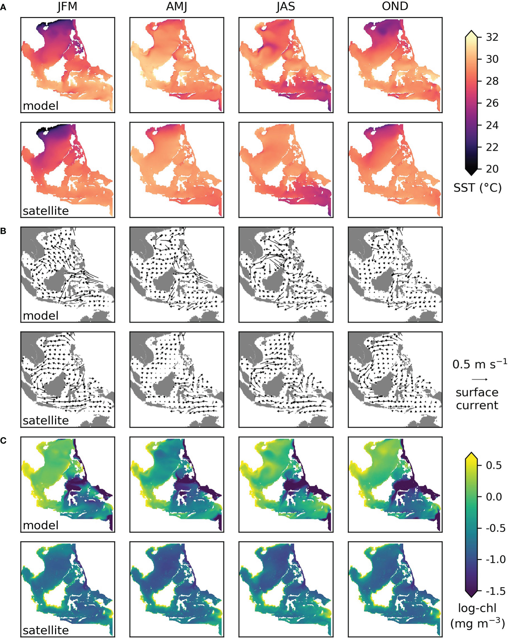
Figure 2 Three-month mean conditions for 1998-2017 from the model (upper row) and derived from satellite observations (lower row) for (A) sea surface temperature, (B) surface current speed and direction, (C) surface chlorophyll-a concentration. JFM=January-February-March etc. The satellite-based products are OSTIA reprocessed sea surface temperature, geostrophic+Ekman surface current and Ocean Colour CCI chlorophyll-a, see section 2.6 for details.
Climate change was applied by using publicly available outputs from the Coupled Model Intercomparison Project Phase 5 (CMIP5; Taylor et al., 2011), a set of climate model experiments performed using protocols agreed by the World Climate Research Programme which inform the Fifth Assessment Report of the Intergovernmental Panel on Climate Change (IPCC, 2021). Lateral boundary conditions were taken from the global model HadGEM2-ES (Jones et al., 2011, sourced from the Earth System Grid Federation archive, https://esgf-index1.ceda.ac.uk/projects/esgf-ceda/) and surface conditions from a regionally-downscaled atmospheric model driven by the same global model, HadGEM2-ES-RCA4, which was sourced from CORDEX Southeast Asia (http://www.ukm.my/seaclid-cordex/; Tangang et al., 2020). This pair of models was selected from the limited set available at the time the modelling was started, in 2019, because it provided both physical and biogeochemical boundary values in the ocean and a physically consistent regional-scale atmospheric component. The atmospheric model provided data at 0.22° resolution: temperature, pressure, wind and humidity at 6-hourly intervals and precipitation and radiation flux at daily frequency. The ocean model provided monthly values of temperature, salinity and current speed at 1° spatial resolution. It also provided annual concentrations of nitrate and inorganic carbon; these were then used to derive concentrations of phosphate and silicate and the monthly cycle of variation using ratios based on the present-day climatology from the World Ocean Atlas 2013 (Garcia et al., 2013a). The atmospheric and oceanic model values were used directly, without bias correction, to retain internal consistency. Atmospheric carbon dioxide levels for climate scenarios were set to the global levels defined for RCP4.5 and RCP8.5 (Meinshausen et al., 2011) for 2006 onwards and to the historical values used in CMIP5 for earlier years.
River inputs of fresh water and nutrients used average present-day values from the global model NEWS2 (Mayorga et al., 2010). Fixed values were used for nutrient concentrations; discharge values were adjusted to give a daily climatology based on historic flows reported by Dai et al. (2009). Future values for riverine discharge were based on this climatology, adjusted each year in line with domain-average precipitation. No information about future changes in river water quality was available, therefore concentrations of nutrients were kept constant at present-day values.
Initial conditions of temperature, salinity, oxygen and nutrients were taken from the World Ocean Atlas 2013 (Locarnini et al., 2013; Zweng et al., 2013; Garcia et al., 2013a; Garcia et al., 2013b) and total alkalinity and dissolved inorganic carbon from the GLODAPv2.2016b gridded dataset (Key et al., 2015; Lauvset et al., 2016). The model was run for an 11-year spin-up period using repeating yearly surface and boundary conditions which were the average for 1971-1980; at the end of the spin period conditions in both physical and ecosystem variables were stable. The model was then run for the period 1971-2098. For 1971-2005 the boundary and surface conditions came from the historical experiment of HadGEM2-ES and HadGEM2-ES-RCA4; for 2006-2098 the RCP4.5 and RCP8.5 experiments were used.
Model outputs were compared to observations to assess how well the model reproduces real-world conditions. Three-month mean conditions for sea surface temperature, currents and chlorophyll were plotted using values from the model and from satellite observations as listed in section 2.6; satellite values were masked to match the model domain, to make visual comparison easier. The period included was 1998-2017 in each case, to give a consistent 20-year period when satellite data were available. The modelled trends in sea surface temperature, surface chlorophyll, dissolved oxygen, net primary production and surface pH were compared to values from satellite observations and from the literature. The comparison period varied to use the longest observational dataset available in each case. The model trend was found by using a linear fit to the monthly mean values for the whole region. For all the comparison to observations, the model values for 2006-2017 were taken from the RCP8.5 run; the results using RCP4.5 were also calculated but were very similar and are not included here. Further comparison to in situ observations of temperature, salinity, nitrate, phosphate and oxygen from the World Ocean Database is provided in the supplementary material.
Present and future values for sea surface temperature and column total net primary production were compared using twenty-year averages for the present-day (2000-2019), mid-century (2040-2059) and end-century (2079-2098) and time series of annual mean values for 1980-2098. The present-day averages used RCP8.5 for 2006 onwards; tests with RCP4.5 gave very similar values. Annual mean values were calculated for the whole domain and for the sample areas shown in Figure 1; anomalies were calculated from these as the difference between the annual value and the mean for 1980-2005, i.e. the historical period as defined for CMIP5.
Mid-century and end-century change in a wider range of variables was summarized by calculating:
1. monthly mean values for each sample area, for 2000-2019, 2040-2059 and 2079-2098;
2. the mean difference between future and present for each area, period and RCP;
3. the present-day range, defined as the difference between the largest and smallest monthly mean value for 2000-2019;
4. a dimensionless index of change, defined as the ratio of the future-present difference to the present-day range;
5. the significance of the change, using a t-test of the null-hypothesis that current and future conditions are the same (Kay and Butenschön, 2018).
The index of change enables the change in different variables to be compared to each other and to the range of conditions experienced in the present day: change that goes significantly outside the current range is likely to put more stress on organisms and ecosystems. The variables included were selected to give a range of ecosystem-relevant parameters: surface and bottom temperature, surface salinity, column total net primary production, phytoplankton biomass and zooplankton biomass and surface and bottom level oxygen and pH.
It was only possible to downscale one model in this study, but in order to put the outputs in the context of other modelling work they have been compared to a range of global model outputs from the CMIP5 set, including the model that is the parent for the regional modelling, HadGEM2-ES. The global model outputs were interpolated to the model grid using a nearest-neighbor method, then masks were applied to select the sample areas shown in Figure 1. Mean values for each area were calculated and compared to regional values and to satellite; these are shown as anomalies in section 3 and as absolute values in the Supplementary Material. The Supplementary Material also includes some comparison of the global model outputs to satellite and in situ observations.
Satellite-derived products sourced from the Copernicus Marine Service (https://marine.copernicus.eu) were used to make plots comparing the model outputs to observations:
● sea surface temperature from multi-sensor satellite and in situ observations (OSTIA, Good et al., 2020, https://doi.org/10.48670/moi-00168);
● surface currents derived by combining geostrophic currents calculated from satellite altimetry with Ekman current from wind reanalysis (Copernicus Globcurrent, Rio et al., 2014, https://doi.org/10.48670/moi-00050);
● surface chlorophyll concentration (ESA Ocean Colour CCI, Sathyendranath et al., 2019, https://doi.org/10.48670/moi-00283);
● column total net primary production (GlobColour, https://doi.org/10.48670/moi-00281).
The same sea surface temperature and chlorophyll products were used for quantitative assessment of trends over time (Table 1). Information about trends in dissolved oxygen, net primary production and surface pH was derived from the literature and sources are given in Table 1.
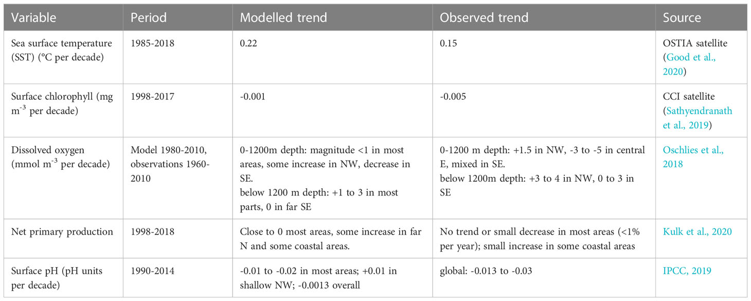
Table 1 Comparison of modelled and observed past trends in selected variables.
CMIP5 global model outputs were sourced from the Earth System Grid Federation portal (https://esgf-index1.ceda.ac.uk/projects/esgf-ceda/).
Section 3.1 shows how the model outputs compare to observed values and trends for the period 1980-2018; section 3.2 presents projections for future values up to the year 2100.
Three-month average modelled surface temperature, currents and chlorophyll for 1998-2017 compared to satellite-derived values are shown in Figure 2. The mean and seasonal variation in sea surface temperature is generally captured well by the model, the exceptions are that April-June (AMJ) temperatures are higher than observed in the west and July-September (JAS) temperatures are lower than observed in the north (Figure 2A). Surface current speeds are higher than satellite derived (geostrophic + Ekman) currents, but the observed circulation patterns are captured by the model, including seasonal reversal due to the monsoon climate in the north of the region (Figure 2B). The range of surface chlorophyll is much greater than observed by satellite, with higher highs and lower lows (Figure 2C). However, the spatial and temporal variations are similar, with the highest values along coasts, especially in the southwest and southeast, and the higher chlorophyll months being October to March in the northern part of the region and July to September in the south.
Compared to the parent global model, chlorophyll estimates by the regional model tend to be closer to satellite values at the coastal sites but not in open waters (Figure S2).
Table 1 shows long-term trends from the model compared to values from satellite observations and reported in the literature. The model outputs and satellite observations both show a rising trend in sea surface temperature for the period 1985-2019, though the observed trend is smaller than modelled (see also Figure 3). The magnitude of change in surface chlorophyll concentration for 1998-2017 is small in both model outputs and satellite observations. Modelled trends in dissolved oxygen concentration are smaller than observed but have the same spatial distribution, with increases in the north and west and decreases in the south and east. The model outputs show little or no change in net primary production since 1998, which is consistent with the findings for this region in a global analysis of satellite and in situ observations (Kulk et al., 2020). The model shows a small decrease in surface pH, -0.01 to -0.02 pH units per decade, except for shallow areas in the northwest of the region where there is a small increase. There are few measurements of pH for the Southeast Asia region to compare this with, but the IPCC reports a global decrease of 0.013 to 0.03 pH units per decade for 1990-2014 (IPCC, 2019).
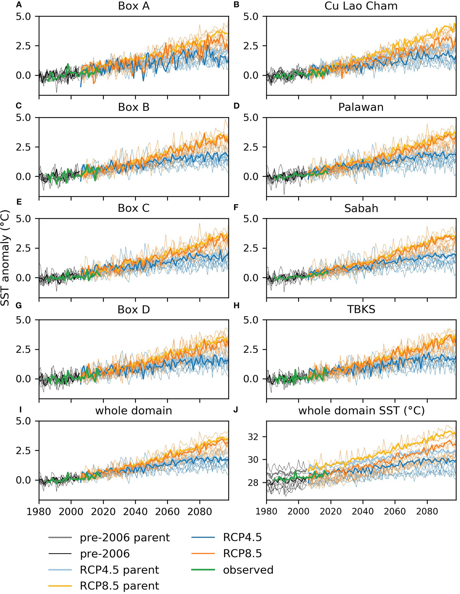
Figure 3 Annual mean sea surface temperature for the sample areas defined in Figure 1: (A-I) anomalies compared to the mean for 1980-2005 averaged over sample areas and the whole domain and (J) annual average for 1980-2098 for the whole domain. The darker lines show the regional model outputs, the paler color lines show the parent global model, the thinner lines show a range of other CMIP5 models. In each case the black lines show the CMIP5 historical period, 1980-2005, the blue lines RCP4.5 and the orange lines RCP8.5. The green line shows satellite-based values, see section 2.6 for product details.
Further comparison to in situ observations is given in the supplementary material. Overall, the model outputs show a reasonable match to the range and median of observations (Figure S3). Agreement is worst for Box A, where temperatures and oxygen are underestimated and nitrate is overestimated. Nutrients are also overestimated in Box C.
This section presents model outputs for conditions to the end of the 21st century under the moderate RCP4.5 scenario (atmospheric greenhouse gas concentrations rising until mid-century and then stabilizing) and the more extreme RCP8.5 (greenhouse gases continuing to rise throughout the century). Sea surface temperature and column total net primary production are discussed in some detail; change in other environmental variables is summarized and discussed more briefly.
Surface temperatures are projected to rise by 1 to 1.5°C by mid-century and 2 to 3°C by end century under RCP8.5, when compared to 2000-2019 (Figures 3, 4). Smaller increases are projected under RCP4.5, i.e. 0.5 to 1°C and 1 to 1.5°C respectively. These changes are in line with those projected by a range of CMIP5 global models, though they are at the high end of the model range (Figure 3), and they imply that temperatures that were average for the region in 2000-2019 would occur only in the very far north by the end of the century under RCP8.5 (see the contours in Figure 4). Change under RCP4.5 is substantially smaller, with end-century conditions similar to those at mid-century under RCP8.5.
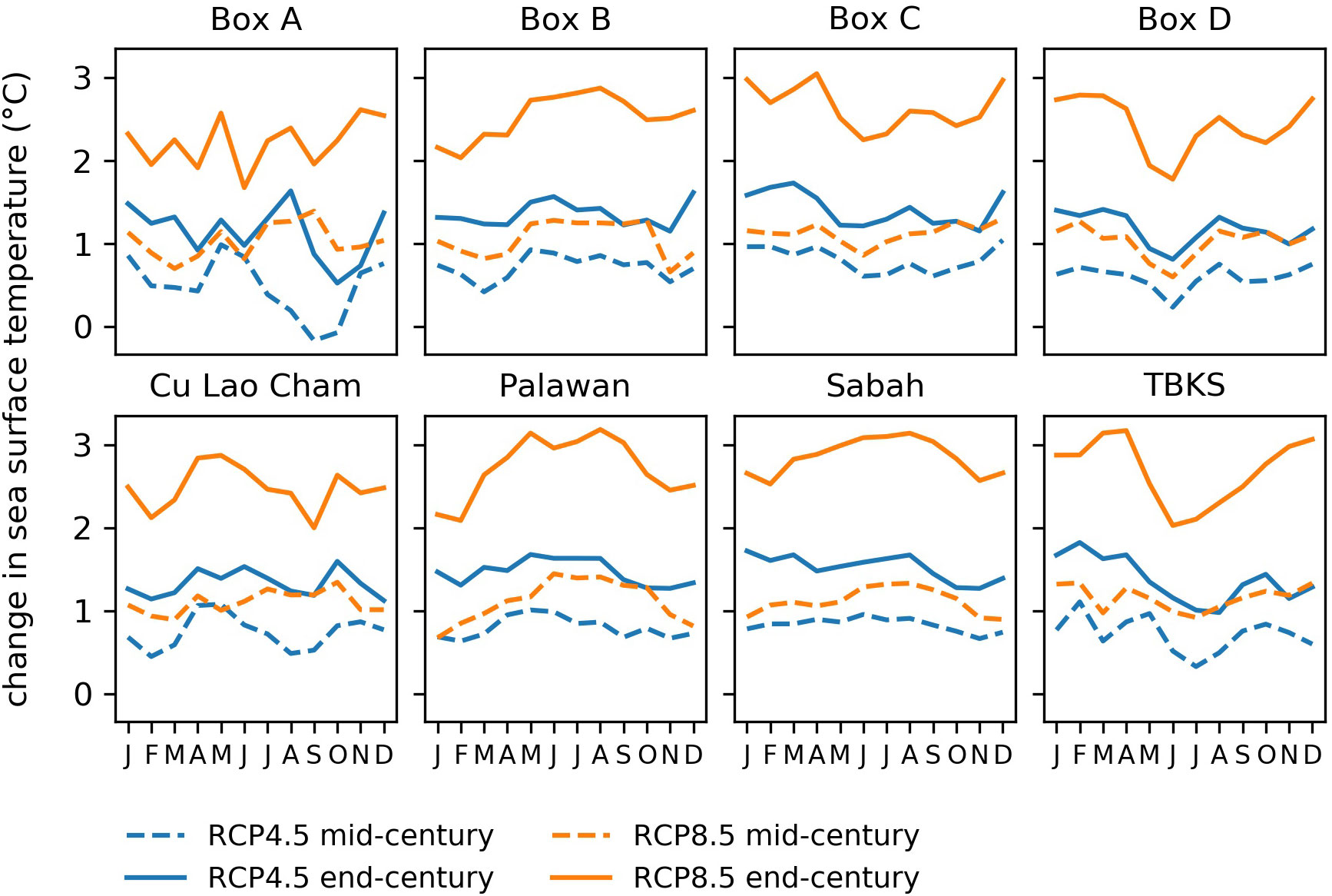
Figure 4 Projected change in monthly mean sea surface temperature compared to present day for 8 sample areas, for mid-century (dashed lines) and endcentury (solid lines). Blue lines show RCP4.5 and orange lines RCP8.5. Temperatures are averaged over 20-year time periods:2000-2019, 2040-2059 and 2079-2098. See Figure 1 for sample area locations.
Among the sample areas, the largest temperature changes are seen in the center and south: Box C, Palawan, Sabah and Taka Bonerate-Kepulauan Selayar (Figures 3, 5). The temperature rise in the regional model is generally similar to that shown by the parent global model and at the high end of the CMIP5 range (Figure 3). However, there are differences in some locations, notably in Cu Lao Cham where the increase shown by the global model at end-century is more than 0.5°C greater than the regional model (Figure 3B). Looking at temperature values rather than anomalies (Figure 3J), the regional model has consistently lower temperatures than the parent global model for the domain as a whole and is in better agreement with satellite values. The same is true for the sample areas, though the size of the difference varies between locations: for Palawan and Sabah there is nearly 2°C difference between the regional and global model, for Box B and Box C the difference is small (shown in the supplementary material, Figure S4).
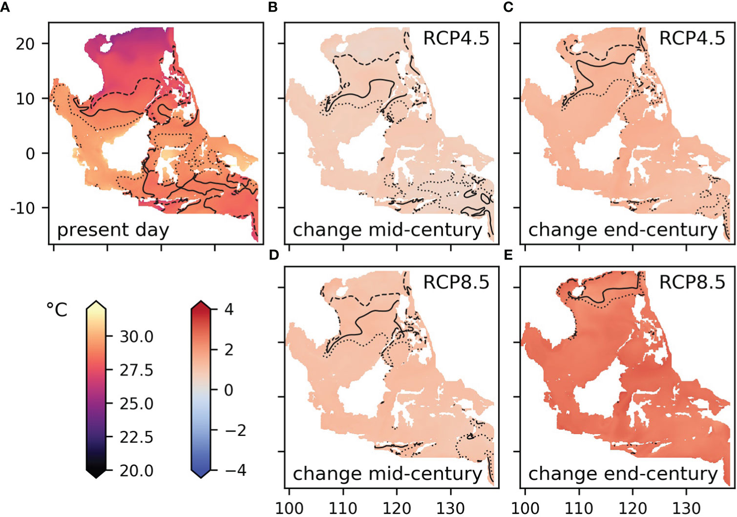
Figure 5 Modelled sea surface temperature: (A) mean for the present day (2000-2019), (B, D) difference between the mid-century (2040-2059) mean and the 2000-2019 mean under RCP4.5 and RCP8.5, (C, E) difference between the end-century (2079-2098) mean and the 2000-2019 mean under RCP4.5 and RCP8.5. The solid black contour shows the median temperature for the present day, the dashed line the 25th quartile and the dotted line shows the 75th quartile.
We looked at the change in monthly mean sea surface temperatures averaged over 20 years to investigate any change in the seasonal cycle (Figure 5). Palawan shows a greater intra-annual change than other areas, with temperatures rising more in April-September than in October-March. The southernmost areas, Box D and Taka Bonerate-Kepulauan Selayar, also show a seasonal change, with smaller temperature rises in May-September than the rest of the year.
This section considers change in net primary production totaled over the whole water column at each grid point. The model shows a general trend to increasing net primary production in the north and south of the region, and either staying stable or decreasing in the center (Figure 6). Projected changes are smaller in relation to the interannual range than for sea surface temperature, and in many sample areas are difficult to distinguish from the general variability (Figure 7). Where changes do appear, they are for RCP8.5 at the end of the century, and this pattern is consistent enough to show up in the whole-region mean (Figure 7I).
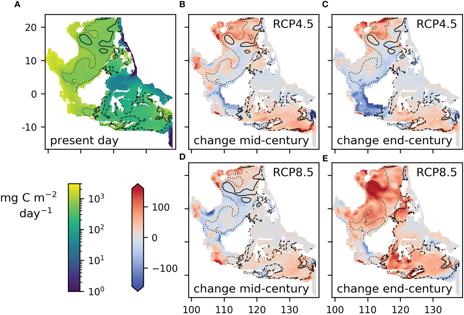
Figure 6 Column total net primary production: (A) mean for the present day (2000-2019), (B, D) difference between the mid-century (2040-2059) mean and the 2000-2019 mean under RCP4.5 and RCP8.5, (C, E) difference between the end-century (2079-2098) mean and the 2000-2019 mean under RCP4.5 and RCP8.5. The solid black contour shows the median for the present day, the dashed line the 25th quartile and the dotted line the 75th quartile.
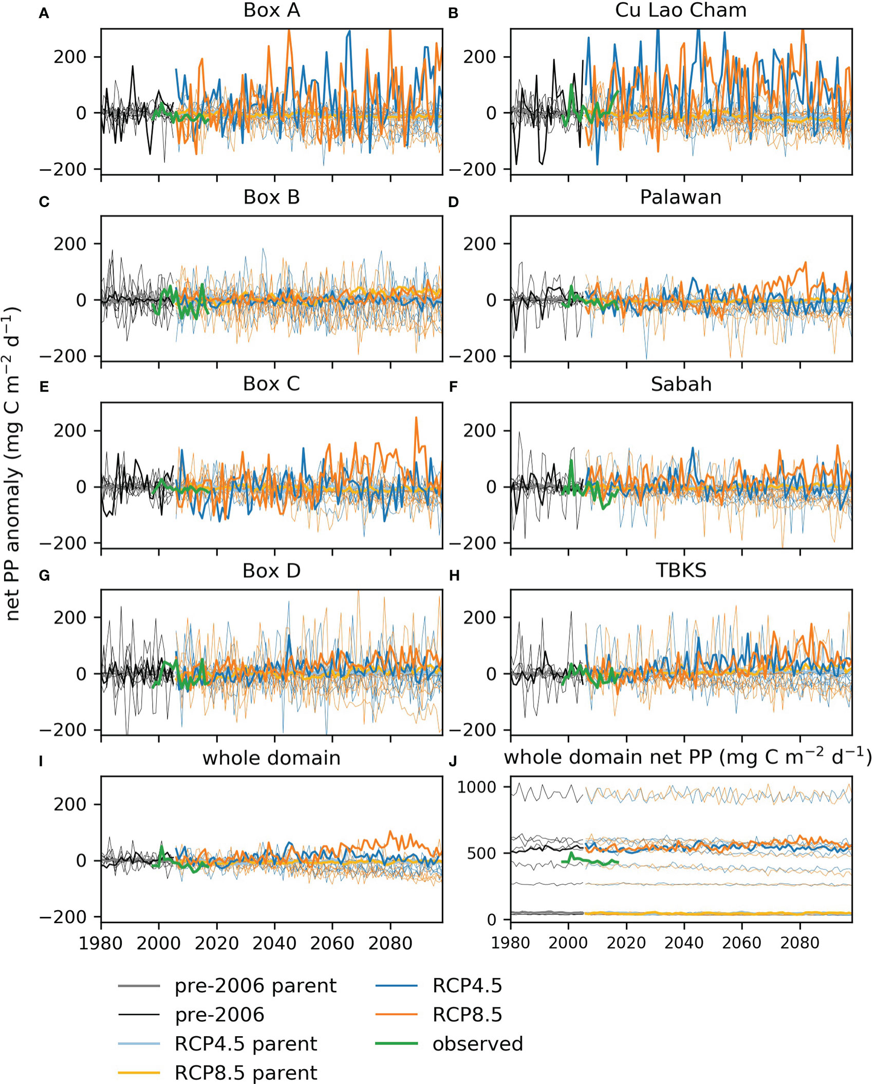
Figure 7 Column total net primary production for the sample areas defined in Figure 1: (A–I) anomalies compared to the mean for 1980-2005 averaged over sample areas and the whole domain and (J) annual average for 1980-2098 for the whole domain. The darker lines show the regional model outputs, the paler color lines show the parent global model, the thinner lines show a range of other CMIP5 models. In each case the black lines show the CMIP5 historical period, 1980-2005, the blue lines RCP4.5 and the orange lines RCP8.5. The green line shows satellite-based values, see section 2.6 for product details.
The global models we used vary widely in their levels of primary production (Figure 7J): the variation between models is much larger than any trend over time or interannual variation. The parent global model has one of the lowest estimates of net primary production, whereas the regional model values are in the middle of the range of the CMIP5 models sampled here, though higher than the majority. This is true for all the sample areas, except in the north (Box A, Cu Lao Cham), where regional model production is higher than all but one of the global models tested (Figure S5).
Some changes in seasonality are projected (Figure 8): for example, Box A shows smaller increases in production in November to February than the rest of the year; Taka Bonerate-Kepulauan Selayar show larger increases in May to September; Sabah shows decreased production in November to March, except for RCP8.5 end-century when these months show the largest increases.
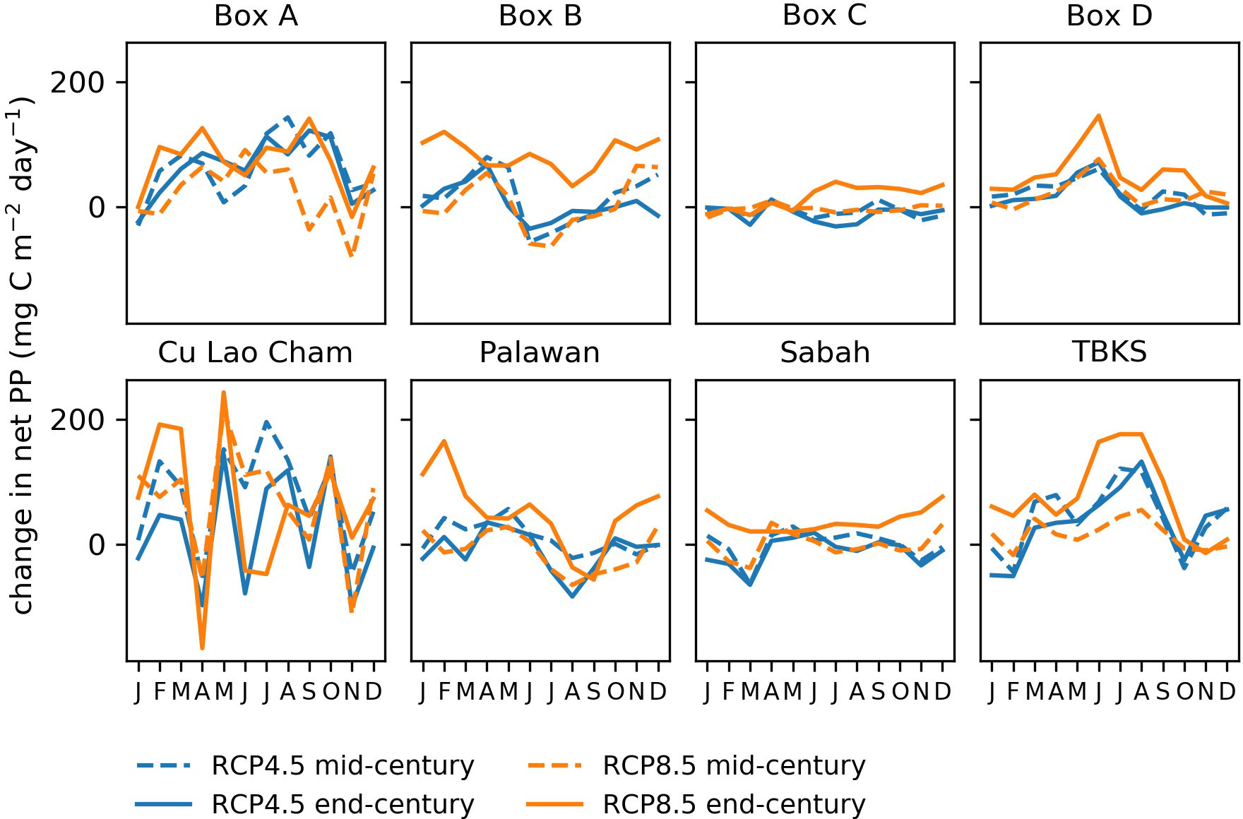
Figure 8 Projected change in monthly mean net primary production compared to present day for 8 sample areas, for mid-century (dashed lines) and end-century (solid lines). Blue lines show RCP4.5 and orange lines RCP8.5. Values are averaged over 20-year time periods: 2000-2019, 2040-2059 and 2079-2098. See Figure 1 for sample area locations.
Overall the best estimate is of little change in net primary production, however there are indications that RCP8.5 at the end of the century shows a different state from earlier periods or from the lower carbon scenario RCP4.5.
The projected 21st century change in other key variables is summarized in Figure 9. This compares monthly mean conditions for 20 years at the start, middle and end of the century (2000-2019, 2040-2059 and 2079-2098). The values show the mean difference between start and mid or end-century, shown in grey where the difference is not statistically significant (p>0.05, t-test, n=240). The colors show the size of the change relative to the present-day variability, defined as the difference between the minimum and maximum monthly values for 2000-2019. Statistically significant change is seen in temperature, surface salinity and bottom-level oxygen for both greenhouse gas scenarios: temperatures rising and salinity and oxygen falling, with larger changes for RCP8.5 than for RCP4.5. There is a significant increase in primary production under RCP8.5 at the end of the century, relative to the present, but not by mid-century; changes under RCP4.5 are smaller and more regionally variable. Surface pH predominantly decreases, most severely toward the end of the century and under RCP8.5. The pattern for phytoplankton and zooplankton biomass is less consistent: there is a broad trend to decreasing biomass under RCP4.5 and increasing under RCP8.5, but the changes are only significant in a few places and well within current variability everywhere. Compared to present-day variability, the bottom level changes are larger than for the sea surface, because bottom-level conditions are more stable and the present-day variability is low: these projections show the effects of climate change reaching all depths of the sea. In the areas around Cu Lao Cham, Sabah and Palawan the water is relatively shallow, so bottom level conditions are more variable than for the other areas and the relative change is smaller.
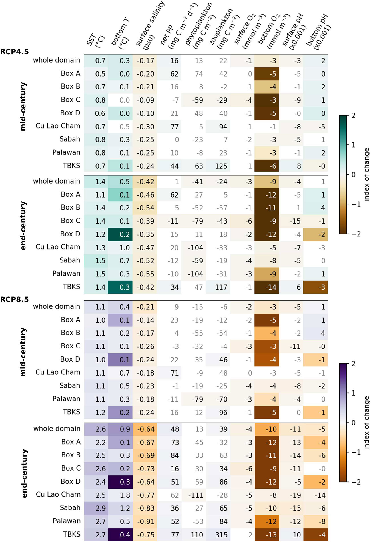
Figure 9 Summary of projected change in selected variables under RCP4.5 (above) and RCP8.5 (below), for the whole domain and sample areas shown in Figure 1. In each case the upper part shows change at mid-century (2040-2059 compared to 2000-2019), the lower part shows end-century change (2079-2098 compared to 2000-2019). Values for primary production, phytoplankton and zooplankton are totals for the water column. Text in grey means the change is not statistically significant. The index of change shows how large the change is compared to the present-day range of monthly mean values.
The projections show seas in Southeast Asia warming at the surface by 1.1-2.9°C on average over the 21st century, with dissolved oxygen decreasing by 5 to 13 mmol m-3 and with pH falling especially under RCP8.5 conditions. The changes reach all parts of the water column and the bottom levels, in particular, are projected to experience conditions well outside the range seen at the start of the century (Figure 9). Changes in the biological system (plankton biomass, primary production) are projected to be smaller than in physical and chemical conditions, but are still significant in some places, especially for the more extreme RCP8.5 scenario. In some locations there are likely to be seasonal changes, with warmer seasons rising in temperature more than cooler seasons. There is considerable variation between the different sample areas, emphasizing the value of using a regional model that can resolve spatial scales and physical and biogeochemical processes that are not included explicitly in global models. Examples of such processes include tidal mixing, the interaction of multiple plankton functional types and nutrient limitation by nitrogen or phosphorus independently, all of which tend to be more important in productive coastal seas than in the open ocean (Drenkard et al., 2021).
Overall, the agreement between modelled and observed values and trends for the period 1980-2018 provides sufficient support for use of the future projections. The good match to the spatial variation and trend in sea surface temperature seen in satellite observations gives confidence in the use of the model outputs for understanding the future physical environment. The modeled rate of increase is somewhat higher than observed, and at the high end of the CMIP5 range, suggesting that the outputs should be treated as towards the high-temperature end of the possible range of futures. Agreement with observation is less close for biogeochemical variables than for physical, as is common in this type of modelling, but spatial and temporal trends are captured. The details of projected change in different variables for different locations should be treated as tentative, but they can give an indication of the types and magnitude of change to be expected and a more nuanced picture than that available from global models. The wide range of biogeochemical outputs from the CMIP5 models included here (Figure 3J, Figure S5) shows how difficult it is to draw confident conclusions about the future biogeochemical environment in regional seas from global projections.
Warming seas mean that by the end of this century some parts of the Southeast Asian seas may experience average temperatures not seen in the region at present (Figure 4). Species that live at or near the sea floor are particularly likely to experience conditions of temperature, oxygen and pH outside the current range of variability, to which they may not be adapted (Figure 9). As a response to rising temperatures, some species populations may be able to move with the present-day temperature contours, seeking to maintain optimum conditions for their growth, reproduction and survival (Pinsky et al., 2013; Poloczanska et al., 2013). However, this adaptation strategy has limited success near warmer regions of species distributions, and does not apply to all types of species, especially sessile organisms – for example, range expansion of corals is restricted because they rely on the tolerance range of their algal symbionts to adapt to new environments (Tonk et al., 2013), and these symbiotic algae are tightly dependent on light and temperature near the sea surface.
All the environmental changes mentioned throughout this article will have consequences for the fisheries sector. This is critical in a region where there are already significant challenges due to overcapacity and declining catches, exacerbated by poorly regulated fisheries (Pomeroy, 2012; Teh et al., 2017). Further modelling is needed to assess the implications of climate change for different species, and the projections presented here could provide input data for such modelling. We can expect that populations of reef-dwelling species such as grouper are likely to decline and small pelagics such as sardine, clupeides and mackerel will re-distribute in response to changes in habitat conditions. Therefore fishers may need to travel further to find their target species, shift to catching different species, perhaps requiring an investment in alternative gear or larger vessels, or in the worst cases be faced with declining catches and no incoming new species (Barange et al., 2018). This is especially a concern in equatorial regions, such as Southeast Asia, where declining local diversity resulting from poleward retreat of distribution leading edges is not necessarily compensated by new species arrivals. Therefore, adapting to climate change will be a significant challenge, especially for the many small-scale fishers in the region, and good management will be essential for protecting livelihoods (Lam et al., 2020). There is a need for modelling of future fish productivity and distribution to inform decision-making.
Increased temperature and reduced salinity, as seen in these projections, may result in increased incidence of harmful algal blooms (HABs). The consequences of such HAB events include reduced water quality and toxin build-up in fish and shellfish, with potential subsequent impacts on human health and food security (GEOHAB, 2010; Gobler, 2020; Young et al., 2020; Trottet et al., 2022). Rising temperatures can also increase the risk of disease in cultured fish (Reverter et al., 2020), shellfish (Allison et al., 2011) and seaweed (Largo et al., 2017), and can lead to a rising number of jellyfish blooms or invasions that may affect aquaculture (Xu et al., 2013; Bosch-Belmar et al., 2020). Changes in the timing of seasons are also likely to affect aquaculture production cycles, where activities are tightly timed to sharp climatic differences between monsoon/inter-monsoon periods. Such changes can be seen in the projected changes for coastal areas, notably Palawan and Taka Bonerate-Kepulauan Selayar (Figure 5). A reduction in the predictability of seasonal cycles often leads to reduced harvests (Handisyde et al., 2006; Hamdan et al., 2015). The projections presented here could be a useful tool for assessing the impacts of climate change on phenology and future potential for aquaculture in different parts of the region.
All the analyzed coastal areas have projected end-century temperature increases close to 1.5°C under RCP4.5, enough to cause thermal stress leading to coral bleaching, while the 2.7°C increase seen under RCP8.5 is likely to cause widespread loss of coral (Lough et al., 2018). The smallest temperature increases were seen at Cu Lao Cham, but at 1.5°C (RCP4.5) or 2.5°C (RCP8.5) even these are too high to prevent coral damage (Dao et al., 2021). Ocean acidification and the overall alteration of the ocean carbonate system resulting from rising atmospheric CO2 levels creates further stress to coral reefs by affecting the ability of reef organisms to maintain sufficient calcification rates in the face of increased dissolution rates and, in extreme cases, prevent the deposition of carbonate minerals needed for skeleton construction through the occurrence of insufficient saturation levels (Eyre et al., 2018). Our projections show surface pH decreasing, though not beyond the range currently experienced; changes in bottom level pH go outside the current range at many locations. Any acidification will act as an additional stressor on coral reefs and make it more difficult for them to recover from bleaching events. The conditions under which coral reefs are able to recover can be complex (Graham et al., 2015) and this has not been considered in the current study.
We were only able to downscale one global model in this work, because of resource constraints and the limited availability of downscaled atmospheric projections at the time the work was started. More regional model projections, based on a range of recent global climate models, are needed to give information about uncertainty. These should follow best practice methods developed from downscaling other regions (Drenkard et al., 2021) including a careful choice of global models to span a range of possible futures, attention to bias correction, and using time periods long enough to capture long-term trends. A downscaled atmospheric model should be used at the surface to capture dynamic features at scales relevant to ecosystem processes; for this region that includes the intense storms associated with tropical cyclones, which are captured better by regional than global models, and monsoon winds influencing coastal upwelling. More regional atmospheric models are now available (Tangang et al., 2020) so it is possible to select from multiple options which have both downscaled atmospheric projections and ocean biogeochemistry from the same global model; in due course this will include downscaled versions of the most recent generation of global models, CMIP6.
A range of regionally-appropriate biogeochemical models should also be used within the regional modelling system. The global model outputs we looked at vary widely in their biogeochemical outputs (Figure 7J, Figure S5), indicating that it would be valuable to include a number of models to get an understanding of the inter-model uncertainty. CMIP6 models include biogeochemical components with greater complexity (Kearney et al., 2021) which could potentially represent the region better, and it would be useful to explore their range of response for Southeast Asia and compare them to CMIP5. But it will also be important to explore the outputs of different models used within a regional modeling system that can simulate the shallow shelf waters and steep slopes of the seas in this region.
Future regional modelling work can build on the results reported here. A useful next step would be to investigate the reasons for the over-prediction of nutrients in the north of the region. Possible causes include inaccurate initial conditions, giving persistently high subsurface nutrients available to be mixed into the eutrophic layer (Figure S3), an over-supply of river-borne nutrients, or overly strong surface currents (Figure 2) leading to too much mixing of nutrients from below. It would also be useful to have information about projected future change in river water quality, especially for large rivers such as the Mekong. This is likely to have high uncertainty, but the sensitivity of the system to river inputs can still be explored.
A further aspect of regional modelling that would benefit from improvement is future changes in storminess, which is of high concern for people in the region. Typhoons disrupt ocean ecosystems through water column mixing by strong winds and the freshening effect of heavy rain. They can also cause flooding and surging which may damage fishing gear and cages and cause long-term damage to coral reefs and other habitats (Harmelin-Vivien, 1994; Latypov and Selin, 2012; Safuan et al., 2020). Increased typhoon activity leads to beach erosion, causing damage to infrastructure and property for communities living close to the shore (Shariful et al., 2020). All of these effects are exacerbated by sea level rise, which poses an additional threat to the large coastal population of this region (Rowley et al., 2007; Neumann et al., 2015; Saleh and Jolis, 2018). There are indications that climate change is resulting in the increased intensity and frequency of typhoons and flooding in SE Asia (Loo et al., 2015), although considerable uncertainty remains about both historical and future trends (Lee et al., 2012; Ying et al., 2012; Knutson et al., 2020). Regional models can simulate stronger storms than global models, because they have higher resolution, but the uncertainty in the projections remains high. We investigated the surface wind speeds in the regional atmospheric model HadGEM2-ES-RCA4, which was used as input to the marine model reported here, for any changes in the strength, frequency or timing of storms. There was some indication of an increase in the number of days per year with strong winds, but not in maximum wind strength or in the pattern across the year. By contrast, Herrmann et al. (2020), based on a much more thorough analysis of outputs from a similar regional model (CNRM-CM5_RegCM4), found a decrease in projected wind speeds, in most of the region and all seasons, except for some increase in average speeds for December to February in the north of the region. The number of tropical cyclones also decreased in all seasons. More work is needed to resolve this uncertainty.
This study, using a single regional-scale model driven by a single global climate model, provides useful, novel information about the potential scale of climate change effects that may occur in the marine environment at different locations across Southeast Asia. However, it does not provide any quantitative indication of the certainty in these changes, which is of key importance for decision-making. Further projections are needed, using a range of models with different climate sensitivities, different biogeochemical components and alternative global emission scenarios, to estimate the uncertainty and give confidence levels in the change projected for different variables and different locations. In a region of exceptionally high marine biodiversity, and where the sea supports the livelihoods of millions of people, such projections are an important tool for communities and policymakers as they plan how they will adapt to the challenge of climate change.
The datasets presented in this study can be found in online repositories. The names of the repository/repositories and accession number(s) can be found below: Zenodo https://zenodo.org/record/4775853.
SK planned the work, carried out the modelling and analysis and led the writing. All authors contributed to the article and approved the submitted version.
This work has received funding in part from the Global Challenges Research Fund (GCRF) via the United Kingdom Research and Innovation (UKRI) under grant agreement reference NE/P021107/1 to the Blue Communities project.
We would like to thank the two reviewers, whose comments greatly improved the manuscript.
Author BG was employed by B. Gonzales Environmental Research and Management Consultancy.
The remaining authors declare that the research was conducted in the absence of any commercial or financial relationships that could be construed as a potential conflict of interest.
All claims expressed in this article are solely those of the authors and do not necessarily represent those of their affiliated organizations, or those of the publisher, the editors and the reviewers. Any product that may be evaluated in this article, or claim that may be made by its manufacturer, is not guaranteed or endorsed by the publisher.
The Supplementary Material for this article can be found online at: https://www.frontiersin.org/articles/10.3389/fmars.2023.1082170/full#supplementary-material
Allison E. H., Badjeck M.-C., Meinhold K. (2011). “The implications of global climate change for molluscan aquaculture,” in Shellfish aquaculture and the environment (West Sussex: John Wiley & Sons, Ltd), 461–490. doi: 10.1002/9780470960967.ch17
Barange M., Bahri T., Beveridge M.C.M, Cochrane K.L., Funge-Smith S., Poulain F. eds. (2018) Impacts of climate change on fisheries and aquaculture: Synthesis of current knowledge, adaptation and mitigation options. FAO fisheries and aquaculture technical paper no. 627 (Rome, Italy: FAO). Available at: http://www.fao.org/publications/card/en/c/I9705EN (Accessed February 18, 2023).
Barange M., Merino G., Blanchard J. L., Scholtens J., Harle J., Allison E. H., et al. (2014). Impacts of climate change on marine ecosystem production in societies dependent on fisheries. Nat. Clim. Change 4, 211–216. doi: 10.1038/nclimate2119
Blackford J. C., Allen J. I., Gilbert F. J. (2004). Ecosystem dynamics at six contrasting sites: a generic modelling study. J. Mar. Syst. 52, 191–215. doi: 10.1016/j.jmarsys.2004.02.004
Blanchard J. L., Jennings S., Holmes R., Harle J., Merino G., Allen J. I., et al. (2012). Potential consequences of climate change for primary production and fish production in large marine ecosystems. Phil. Trans. R. Soc B 367, 2979–2989. doi: 10.1098/rstb.2012.0231
Bosch-Belmar M., Milisenda G., Basso L., Doyle T. K., Leone A., Piraino S. (2020). Jellyfish impacts on marine aquaculture and fisheries. Rev. Fisheries Sci. Aquaculture 0, 1–18. doi: 10.1080/23308249.2020.1806201
Burke L., Reytar K., Spalding M., Perry A. (2012) Reefs at risk revisited in the coral triangle (World Resources Institute). Available at: https://www.wri.org/publication/reefs-risk-revisited-coral-triangle (Accessed February 13, 2021).
Burke L., Selig (WRI) L., Spalding, UNEP-WCMC, M., Cambridge, and UK (2002) Reefs at risk in southeast Asia. Available at: https://www.wri.org/publication/reefs-risk-southeast-asia (Accessed February 13, 2021).
Butenschön M., Clark J., Aldridge J. N., Allen J. I., Artioli Y., Blackford J., et al. (2016). ERSEM 15.06: a generic model for marine biogeochemistry and the ecosystem dynamics of the lower trophic levels. Geosci. Model. Dev. 9, 1293–1339. doi: 10.5194/gmd-9-1293-2016
Cesar H., Burke L., Pet-Soede L. (2003) The economics of worldwide coral reef degradation (Cesar Environmental Economics Consulting). Available at: https://www.wwf.or.jp/activities/lib/pdf_marine/coral-reef/cesardegradationreport100203.pdf (Accessed February 7, 2021).
Dai A., Qian T., Trenberth K. E., Milliman J. D. (2009). Changes in continental freshwater discharge from 1948 to 2004. J. Climate 22, 2773–2792. doi: 10.1175/2008JCLI2592.1
Dao H. N., Vu H. T., Kay S., Sailley S. (2021). Impact of seawater temperature on coral reefs in the context of climate change. a case study of Cu lao cham – hoi an biosphere reserve. Front. Mar. Sci. 8. doi: 10.3389/fmars.2021.704682
Drenkard E. J., Stock C., Ross A. C., Dixon K. W., Adcroft A., Alexander M., et al. (2021). Next-generation regional ocean projections for living marine resource management in a changing climate. ICES J. Mar. Sci. 78, 1969–1987. doi: 10.1093/icesjms/fsab100
Ebarvia M. C. (2016). Economic assessment of oceans for sustainable blue economy development. J. Ocean Coast. Economics 2 (2), 7. doi: 10.15351/2373-8456.1051
Eyre B. D., Cyronak T., Drupp P., Carlo E. H. D., Sachs J. P., Andersson A. J. (2018). Coral reefs will transition to net dissolving before end of century. Science 359, 908–911. doi: 10.1126/science.aao1118
FAO (2018). The state of world fisheries and aquaculture 2018 - meeting the sustainable development goals (Rome). Available at: http://www.fao.org/3/I9540EN/i9540en.pdf.
Fernandes J. A., Kay S., Hossain M. A. R., Ahmed M., Cheung W. W. L., Lazar A. N., et al. (2016). Projecting marine fish production and catch potential in Bangladesh in the 21st century under long-term environmental change and management scenarios. ICES J. Mar. Sci. 73, 1357–1369. doi: 10.1093/icesjms/fsv217
García H. E., Locarnini R. A., Boyer T. P., Antonov J. I., Baranova O. K., Zweng M. M., et al. (2013a). World Ocean Atlas 2013 Volume 4: Dissolved Inorganic Nutrients (phosphate, nitrate, silicate). Levitus S., Mishonov A., Technical Ed., NOAA Atlas NESDIS 76, 25.
Garcia H. E., Locarnini R. A., Boyer T. P., Baranova O. K., Zweng M. M., Reagan J. R., et al. (2013b). World Ocean Atlas 2013 Volume 3: Dissolved Oxygen, Apparent Oxygen Utilization, and Oxygen Saturation. Levitus S., Mishonov A., Technical Ed., NOAA Atlas NESDIS 75, 29.
GEOHAB (2010) Global ecology and oceanography of harmful algal blooms, harmful algal blooms in Asia (Paris and Newark, Delaware: IOC and SCOR). Available at: http://hab.ioc-unesco.org/index.php?option=com_oe&task=viewDocumentRecord&docID=5460 (Accessed February 7, 2021).
Gobler C. J. (2020). Climate change and harmful algal blooms: Insights and perspective. Harmful Algae 91, 101731. doi: 10.1016/j.hal.2019.101731
Good S., Fiedler E., Mao C., Martin M. J., Maycock A., Reid R., et al. (2020). The current configuration of the OSTIA system for operational production of foundation Sea surface temperature and ice concentration analyses. Remote Sens. 12, 720. doi: 10.3390/rs12040720
Graham N. A. J., Jennings S., MacNeil M. A., Mouillot D., Wilson S. K. (2015). Predicting climate-driven regime shifts versus rebound potential in coral reefs. Nature 518, 94–97. doi: 10.1038/nature14140
Hamdan R., Othman A., Kari F. (2015). Climate change effects on aquaculture production performance in Malaysia: An environmental performance analysis. Int. J. Business Soc. 16 (3). doi: 10.33736/ijbs.573.2015
Handisyde N. T., Ross L. G., Badjeck M.-C., Allison E. H. (2006) The effects of climate change on world aquaculture: A global perspective (Scotland, UK: DFID (Department for International Development). Available at: https://paper/The-Effects-of-Climate-change-on-World-Aquaculture%3A/737a6bc5d5c1d0fa4848bec99b040238ebdfc747 (Accessed February 7, 2021).
Harmelin-Vivien M. L. (1994). The effects of storms and cyclones on coral reefs: A review. J. Coast. Res. 12, 211–231.
Herrmann M., Ngo-Duc T., Trinh-Tuan L. (2020). Impact of climate change on sea surface wind in southeast Asia, from climatological average to extreme events: results from a dynamical downscaling. Clim. Dyn. 54, 2101–2134. doi: 10.1007/s00382-019-05103-6
Hoegh-Guldberg O., Mumby P. J., Hooten A. J., Steneck R. S., Greenfield P., Gomez E., et al. (2007). Coral reefs under rapid climate change and ocean acidification. Science 318, 1737. doi: 10.1126/science.1152509
Holt J., Harle J., Proctor R., Michel S., Ashworth M., Batstone C., et al. (2009). Modelling the global coastal ocean. Phil. Trans. R. Soc A 367, 939–951. doi: 10.1098/rsta.2008.0210
Holt J. T., James I. D. (2001). An s coordinate density evolving model of the northwest European continental shelf 1, model description and density structure. J. Geophys. Res. 106, 14015–14,034. doi: 10.1029/2000JC000304
Holt J., Schrum C., Cannaby H., Daewel U., Allen I., Artioli Y., et al. (2016). Potential impacts of climate change on the primary production of regional seas: A comparative analysis of five European seas. Prog. Oceanography 140, 91–115. doi: 10.1016/j.pocean.2015.11.004
Hughes T. P., Anderson K. D., Connolly S. R., Heron S. F., Kerry J. T., Lough J. M., et al. (2018). Spatial and temporal patterns of mass bleaching of corals in the anthropocene. Science 359, 80–83. doi: 10.1126/science.aan8048
IPCC (2019) IPCC special report on the ocean and cryosphere in a changing climate. Available at: https://www.ipcc.ch/srocc/.
IPCC (2021). Climate change 2021: The physical science basis. Contribution of working group I to the sixth assessment report of the intergovernmental panel on climate change. Eds. Masson-Delmotte V., Zhai P., Pirani A., Connors S. L., Péan C., Berger S., et al (Cambridge, United Kingdom and New York, NY, USA: Cambridge University Press). Available at: https://www.ipcc.ch/report/ar6/wg1/#FullReport.
Jones C. D., Hughes J. K., Bellouin N., Hardiman S. C., Jones G. S., Knight J., et al. (2011). The HadGEM2-ES implementation of CMIP5 centennial simulations. Geoscientific Model. Dev. 4, 543–570. doi: 10.5194/gmd-4-543-2011
Kay S. (2021) Marine environment climate change projections for southeast Asian seas (version 1) [Dataset]. Available at: https://zenodo.org/record/4775853.
Kay S., Butenschön M. (2018). Projections of change in key ecosystem indicators for planning and management of marine protected areas: An example study for European seas. Estuarine Coast. Shelf Sci. 201, 172–184. doi: 10.1016/j.ecss.2016.03.003
Kearney K. A., Bograd S. J., Drenkard E., Gomez F. A., Haltuch M., Hermann A. J., et al. (2021). Using global-scale earth system models for regional fisheries applications. Front. Mar. Sci. 8. doi: 10.3389/fmars.2021.622206
Key R. M., Olsen A., van Heuven S., Lauvset S. K., Velo A., Lin X., et al. (2015). Global ocean data analysis project, version 2 (GLODAPv2). ORNL/CDIAC-162, ND-P093. (Oak Ridge, Tennessee: Carbon Dioxide Information Analysis Center, Oak Ridge National Laboratory, US Department of Energy). doi: 10.3334/CDIAC/OTG.NDP093_GLODAPv2
Knutson T., Camargo S. J., Chan J. C. L., Emanuel K., Ho C.-H., Kossin J., et al. (2020). Tropical cyclones and climate change assessment: Part II: Projected response to anthropogenic warming. Bull. Am. Meteorological Soc. 101, E303–E322. doi: 10.1175/BAMS-D-18-0194.1
Kulk G., Platt T., Dingle J., Jackson T., Jönsson B. F., Bouman H. A., et al. (2020). Primary production, an index of climate change in the ocean: Satellite-based estimates over two decades. Remote Sens. 12, 826. doi: 10.3390/rs12050826
Lam V. W. Y., Allison E. H., Bell J. D., Blythe J., Cheung W. W. L., Frölicher T. L., et al. (2020). Climate change, tropical fisheries and prospects for sustainable development. Nat. Rev. Earth Environ. 1, 440–454. doi: 10.1038/s43017-020-0071-9
Largo D. B., Chung I. K., Phang S.-M., Gerung G. S., Sondak C. F. A. (2017). “Impacts of climate change on eucheuma-kappaphycus farming,” in Tropical seaweed farming trends, problems and opportunities: Focus on kappaphycus and eucheuma of commerce developments in applied phycology. Eds. Hurtado A. Q., Critchley A. T., Neish I. C. (Cham: Springer International Publishing). doi: 10.1007/978-3-319-63498-2_7
Latypov Y. Y., Selin N. (2012). Changes of reef community near Ku lao cham islands (South China Sea) after Sangshen Typhoon. American J. Clim. Change. 1 (1), 41–47. doi: 10.4236/ajcc.2012.11004
Lauvset S. K., Key R. M., Olsen A., van Heuven S., Velo A., Lin X., et al. (2016). A new global interior ocean mapped climatology: the 1° × 1° GLODAP version 2. Earth System Sci. Data 8, 325–340. doi: 10.5194/essd-8-325-2016
Lee T.-C., Knutson T. R., Kamahori H., Ying M. (2012). Impacts of climate change on tropical cyclones in the Western north pacific basin. part I: Past observations. Trop. Cyclone Res. Rev. 1, 213–235. doi: 10.6057/2012TCRR02.08
Locarnini R. A., Mishonov A. V., Antonov J. I., Boyer T. P., Garcia H. E., Baranova O. K., et al. (2013). World Ocean Atlas 2013, Volume 1: Temperature. Levitus S., Mishonov A., Technical Ed., NOAA Atlas NESDIS. 73, 40.
Loo Y. Y., Billa L., Singh A. (2015). Effect of climate change on seasonal monsoon in Asia and its impact on the variability of monsoon rainfall in southeast Asia. Geosci. Front. 6, 817–823. doi: 10.1016/j.gsf.2014.02.009
Lough J. M., Anderson K. D., Hughes T. P. (2018). Increasing thermal stress for tropical coral reefs: 1871–2017. Sci. Rep. 8, 6079. doi: 10.1038/s41598-018-24530-9
Mayorga E., Seitzinger S. P., Harrison J. A., Dumont E., Beusen A. H. W., Bouwman A. F., et al. (2010). Global nutrient export from WaterSheds 2 (NEWS 2): Model development and implementation. Environ. Model. Software 25, 837–853. doi: 10.1016/j.envsoft.2010.01.007
Meinshausen M., Smith S. J., Calvin K., Daniel J. S., Kainuma M. L. T., Lamarque J.-F., et al. (2011). The RCP greenhouse gas concentrations and their extensions from 1765 to 2300. Climatic Change 109, 213. doi: 10.1007/s10584-011-0156-z
Monnier L., Gascuel D., Alava J. J., Barragan M. J., Gaibor N., Hollander F. A., et al. (2020) Small-scale fisheries in a warming ocean: exploring adaptation to climate change (Berlin, Germany: WWF Germany). Available at: https://www.wwf.eu/?956166/Small-scale-fisheries-in-a-warming-ocean (Accessed February 7, 2021).
Neumann B., Vafeidis A. T., Zimmermann J., Nicholls R. J. (2015). Future coastal population growth and exposure to Sea-level rise and coastal flooding - a global assessment. PloS One 10, e0118571. doi: 10.1371/journal.pone.0118571
Oschlies A., Brandt P., Stramma L., Schmidtko S. (2018). Drivers and mechanisms of ocean deoxygenation. Nature Geoscience 11, 467–473. doi: 10.1038/s41561-018-0152-2
Pinsky M. L., Worm B., Fogarty M. J., Sarmiento J. L., Levin S. A. (2013). Marine taxa track local climate velocities. Science 341, 1239–1242. doi: 10.1126/science.1239352
Poloczanska E. S., Brown C. J., Sydeman W. J., Kiessling W., Schoeman D. S., Moore P. J., et al. (2013). Global imprint of climate change on marine life. Nat. Clim. Change 3, 919–925. doi: 10.1038/nclimate1958
Pomeroy R. S. (2012). Managing overcapacity in small-scale fisheries in southeast Asia. Mar. Policy 36, 520–527. doi: 10.1016/j.marpol.2011.10.002
Reverter M., Sarter S., Caruso D., Avarre J.-C., Combe M., Pepey E., et al. (2020). Aquaculture at the crossroads of global warming and antimicrobial resistance. Nat. Commun. 11, 1870. doi: 10.1038/s41467-020-15735-6
Rio M.-H., Mulet S., Picot N. (2014). Beyond GOCE for the ocean circulation estimate: Synergetic use of altimetry, gravimetry, and in situ data provides new insight into geostrophic and ekman currents. Geophysical Res. Lett. 41, 8918–8925. doi: 10.1002/2014GL061773
Rowley R. J., Kostelnick J. C., Braaten D., Li X., Meisel J. (2007). Risk of rising sea level to population and land area. Eos Trans. Am. Geophysical Union 88, 105–107. doi: 10.1029/2007EO090001
Safuan C. D. M., Roseli N. H., Bachok Z., Akhir M. F., Xia C., Qiao F. (2020). First record of tropical storm (Pabuk - January 2019) damage on shallow water reef in pulau bidong, south of south China Sea. Regional Stud. Mar. Sci. 35, 101216. doi: 10.1016/j.rsma.2020.101216
Saleh E., Jolis G. (2018). Climate change vulnerability assessment of the tun mustapha park, sabah (Petaling Jaya, Selangor, Malaysia: WWF-Malaysia).
Sathyendranath S., Brewin R. J. W., Brockmann C., Brotas V., Calton B., Chuprin A., et al. (2019). An ocean-colour time series for use in climate studies: The experience of the ocean-colour climate change initiative (OC-CCI). Sensors 19, 4285. doi: 10.3390/s19194285
Shariful F., Sedrati M., Ariffin E., Shubri S. M., Akhir M. (2020). Impact of 2019 tropical storm (Pabuk) on beach morphology, terengganu coast (Malaysia). J. Coast. Res. 95 (sp1), 346–350. doi: 10.2112/SI95-067.1
Stock C. A., Alexander M. A., Bond N. A., Brander K. M., Cheung W. W. L., Curchitser E. N., et al. (2011). On the use of IPCC-class models to assess the impact of climate on living marine resources. Prog. Oceanography 88, 1–27. doi: 10.1016/j.pocean.2010.09.001
Tangang F., Chung J. X., Juneng L., Supari , Salimun E., Ngai S. T., et al. (2020). Projected future changes in rainfall in southeast Asia based on CORDEX–SEA multi-model simulations. Clim Dyn 55, 1247–1267. doi: 10.1007/s00382-020-05322-2
Taylor K. E., Stouffer R. J., Meehl G. A. (2011). An overview of CMIP5 and the experiment design. Bull. Amer. Meteor. Soc 93, 485–498. doi: 10.1175/BAMS-D-11-00094.1
Teh L. C. L., Pauly D. (2018). Who brings in the fish? the relative contribution of small-scale and industrial fisheries to food security in southeast Asia. Front. Mar. Sci. 5. doi: 10.3389/fmars.2018.00044
Teh L. S. L., Witter A., Cheung W. W. L., Sumaila U. R., Yin X. (2017). What is at stake? status and threats to south China Sea marine fisheries. Ambio 46, 57–72. doi: 10.1007/s13280-016-0819-0
Tonk L., Sampayo E. M., Weeks S., Magno-Canto M., Hoegh-Guldberg O. (2013). Host-specific interactions with environmental factors shape the distribution of symbiodinium across the great barrier reef. PloS One 8, e68533. doi: 10.1371/journal.pone.0068533
Trottet A., George C., Drillet G., Lauro F. M. (2022). Aquaculture in coastal urbanized areas: A comparative review of the challenges posed by harmful algal blooms. Crit. Rev. Environ. Sci. Technol. 52, 2888–2929. doi: 10.1080/10643389.2021.1897372
van Vuuren D. P., Edmonds J., Kainuma M., Riahi K., Thomson A., Hibbard K., et al. (2011). The representative concentration pathways: an overview. Climatic Change 109, 5–31. doi: 10.1007/s10584-011-0148-z
Veron J., DeVantier L. M., Turak E., Green A. L., Kininmonth S., Stafford-Smith M., et al. (2011). “The coral triangle,” in Coral reefs: An ecosystem in transition. Eds. Dubinsky Z., Stambler N. (Dordrecht: Springer Netherlands), 47–55. doi: 10.1007/978-94-007-0114-4_5
Xu Y., Ishizaka J., Yamaguchi H., Siswanto E., Wang S. (2013). Relationships of interannual variability in SST and phytoplankton blooms with giantjellyfish (Nemopilema nomurai) outbreaks in the yellow Sea and East China Sea. J. Oceanogr 69, 511–526. doi: 10.1007/s10872-013-0189-1
Ying M., Knutson T. R., Kamahori H., Lee T.-C. (2012). Impacts of climate change on tropical cyclones in the Western north pacific basin. part II: Late twenty-first century projections. Trop. Cyclone Res. Rev. 1, 231–241. doi: 10.6057/2012TCRR02.09
Young N., Sharpe R. A., Barciela R., Nichols G., Davidson K., Berdalet E., et al. (2020). Marine harmful algal blooms and human health: A systematic scoping review. Harmful Algae 98, 101901. doi: 10.1016/j.hal.2020.101901
Keywords: marine ecosystem model, marine biogeochemical model, regional climate modeling, climate change, southeast Asia, biosphere reserve
Citation: Kay S, Avillanosa AL, Cheung VV, Dao HN, Gonzales BJ, Palla HP, Praptiwi RA, Queirós AM, Sailley SF, Sumeldan JDC, Syazwan WM, Then AY-H and Wee HB (2023) Projected effects of climate change on marine ecosystems in Southeast Asian seas. Front. Mar. Sci. 10:1082170. doi: 10.3389/fmars.2023.1082170
Received: 27 October 2022; Accepted: 07 March 2023;
Published: 28 March 2023.
Edited by:
Nathan John Waltham, James Cook University, AustraliaReviewed by:
Hem Nalini Morzaria-Luna, Long Live the Kings, United StatesCopyright © 2023 Kay, Avillanosa, Cheung, Dao, Gonzales, Palla, Praptiwi, Queirós, Sailley, Sumeldan, Syazwan, Then and Wee. This is an open-access article distributed under the terms of the Creative Commons Attribution License (CC BY). The use, distribution or reproduction in other forums is permitted, provided the original author(s) and the copyright owner(s) are credited and that the original publication in this journal is cited, in accordance with accepted academic practice. No use, distribution or reproduction is permitted which does not comply with these terms.
*Correspondence: Susan Kay, c3VrYUBwbWwuYWMudWs=
Disclaimer: All claims expressed in this article are solely those of the authors and do not necessarily represent those of their affiliated organizations, or those of the publisher, the editors and the reviewers. Any product that may be evaluated in this article or claim that may be made by its manufacturer is not guaranteed or endorsed by the publisher.
Research integrity at Frontiers
Learn more about the work of our research integrity team to safeguard the quality of each article we publish.