 Rémi Laxenaire
 Eric P. Chassignet
 Dmitry S. Dukhovskoy
 Steven L. Morey
- 1Center for Ocean-Atmospheric Prediction Studies, Florida State University, Tallahassee, FL, United States
- 2Laboratoire de Météorologie Dynamique, LMD-IPSL, UMR, École Polytechnique, ENS, CNRS, Paris, France
- 3Laboratoire de l’Atmosphère et des Cyclones (LACy, UMR 8105 CNRS, Université de la Réunion, Météo-France), Université de La Réunion, Saint-Denis de La Réunion, France
- 4National Oceanic and Atmospheric Administration, National Weather Service, National Centers for Environmental Prediction, College Park, MD, United States
- 5School of the Environment, Florida Agricultural and Mechanical University, FSH Science Research Center, Tallahassee, FL, United States
The Loop Current (LC), which is the main mesoscale dynamic feature of the Gulf of Mexico (GoM), has a major impact on the circulation and its variability in the interior Gulf. The LC is a highly variable and dynamic feature. It changes shape from a short jet connecting the two openings of the GoM in an almost straight line ("retracted phase") to a long loop invading most of the eastern part of the GoM ("extended phase"). When it is in the extended phase, it can shed large anticyclonic eddies, called Loop Current Eddies, which then migrate to the western GoM. In this study, the processes controlling the LC dynamics are investigated using two multi-decadal simulations of the Gulf of Mexico HYbrid Coordinate Ocean Model differing in their open boundary conditions (BCs) and altimetry-derived gridded fields. The LC in the simulation with BCs derived from monthly climatology state variables frequently remains in its retracted phase significantly longer than observed. In contrast, the duration of the retracted phase is notably shorter in the simulation in which the BCs have realistic daily variability. By examining the flow properties through the Yucatan Channel from which the LC originates, we find that increased intensity of this current and a westward shift of the mean core is associated with the LC transitions from the retracted to the extended phase. This transition is accompanied by an increase of both cyclonicity of the flow in the west and anticyclonicity in the east of the core of this jet. Moreover, the number of anticyclonic eddies entering in the GoM through the Yucatan Channel is significantly higher when the LC extends in the GoM. Consequently, this study demonstrates the importance of realistic flow variability at the lateral boundaries for accurate simulation of the LC system in a model, and reveals characteristics of the upstream flow associated with different LC behavior that can potentially aid in forecasting the LC system.
1 Introduction
The Gulf of Mexico (GoM) is a marginal sea of the Atlantic Ocean partially closed by the United States, the United Mexican States, and the Republic of Cuba. It has an average depth of 1615 m with a maximum depth of 4400 m. The GoM is connected in the south to the Caribbean Sea via the Yucatan Channel (YC) (threshold depth of about 2000 m) and in the east to the Atlantic Ocean via the Strait of Florida (SF) (threshold depth shallower than 1000 m). The main oceanic circulation feature in the GoM is an intense surface jet (up to more than 1 m/s in the upper 800 m), called the Loop Current (LC), which originates in the YC and exits the Gulf through the SF. This current is, like the Gulf Stream, a branch of the western boundary current system of the North Atlantic Ocean and has an average transport between 23 and 31 Sv (e.g., Baringer & Larsen, 2001; Candela et al., 2002; Johns et al., 2002; Sheinbaum et al., 2002; Candela et al., 2019). The LC undergoes large variations as its shape varies from a short jet connecting the two GoM openings (YC and SF) in an almost direct port-to-port fashion (hereafter “retracted phase”) to a long loop invading most the eastern part of the GoM (hereafter “extended phase”) (e.g. seminal work of Reid, 1972). Episodically, the LC sheds large warm-core anticyclonic rings (radius about 200-400 km) called Loop Current eddies (LCEs) (e.g., Cochrane, 1972; Elliott, 1982; Vukovich, 1995; Leben, 2005; Dukhovskoy et al., 2015), but the LC dynamics are also characterized by smaller scale variability that includes meanders (e.g., Vukovich et al., 1979; Ezer et al., 2003; Donohue et al., 2016), and frontal eddies – both cyclonic (e.g., Vukovich & Maul, 1985; Walker et al., 2009; Jouanno et al., 2016) and anticyclonic (e.g., Hamilton et al., 2000; Leben, 2005).
The time interval between two LCE detachments, commonly called the eddy separation period, varies from a few weeks to more than a year and a half (Vukovich, 1995; Sturges & Leben, 2000; Leben, 2005; Schmitz, 2005; Dukhovskoy et al., 2015). Once formed, LCEs propagate westward from the central part of GoM to its western boundary where they slowly dissipate (Leben, 2005). This is in constrast to the frontal eddies that dissipate rapidly as they propagate along the LC (Leben, 2005). Overall, the LC system is the most dominant feature in the Gulf, despite a non-negligible wind-induced circulation (Sturges & Blaha, 1976; Elliott, 1982; Sturges et al., 1993; Olvera-Prado, 2019). In addition, variability in the LC generates topographic Rossby waves (Oey, 2008; Hamilton, 2009) and is correlated with deep water exchanges through the YC. An increase in volume of the LC when it expends is compensated by a the deep outflow in the YC and vice-versa after a shedding event (Maul, 1977; Bunge et al., 2002; Ezer et al., 2003; Lee & Mellor, 2003; Chang & Oey, 2011; Nedbor-Gross et al., 2014). The LC and associated LCEs have been the subject of numerous studies, starting with in-situ observations (Leipper, 1970; Behringer et al., 1977; Maul, 1977) and, with the advent of satellites, synoptic views of surface fields such as temperature (e.g., Maul, 1975) and sea surface height (SSH) (e.g., Leben, 2005). Altimetric sensors are unaffected by cloud cover and several methods have been developed to track the LC and its associated eddies from SSH fields, ranging from simple methods such as identification of the maximum horizontal gradient of SSH (e.g., Lindo-Atichati et al., 2012; Lindo-Atichati et al., 2013) or of an empirical demeaned SSH contour (e.g. 17 cm for Leben, 2005) to more complex techniques using a Kalman filter (Dukhovskoy et al., 2015) or connecting cells associated with the highest absolute surface velocities (Hirschi et al., 2019).
Many studies have attempted to explain the mechanisms controlling the shape of the LC and associated eddy separation. It is not chaotic (Lugo-Fernández, 2007) and idealized numerical models (Hurlburt & Thompson, 1980) together with analytical models (Pichevin & Nof, 1997; Nof & Pichevin, 2001; Nof, 2005) have shown that the detachment of LCEs has a natural separation period controlled by horizontal shear instability and the β-effect and thus that the detachment mechanism does not require external perturbations. However, these studies, as well as those using more complex numerical models and observations, have also shown that the eddy separation period can be modulated by external factors. Several studies emphasized the importance of the GoM inflows and outflows such as their relative magnitude (Pichevin & Nof, 1997; Weisberg & Liu, 2017; Moreles et al., 2021), their fluctuations (Oey et al., 2003; Sturges et al., 2010), their stratification (Moreles et al., 2021) and their vorticity (Candela et al., 2002; Oey, 2004). Vorticity was found to be modulated by mesoscale activity, such as cyclones in the GoM that can either block the invasion of the LC in the Gulf (Schmitz, 2005; Zavala-Hidalgo et al., 2006) or favor the release of LCE (Chérubin et al., 2006), as well as Caribbean Anticyclones (Murphy et al., 1999; Candela et al., 2002; Oey et al., 2003; Athié et al., 2012; Garcia-Jove et al., 2016; Androulidakis et al., 2021; Ntaganou et al.,), or deep eddies (Welsh & Inoue, 2000; Oey, 2008) that influence the dynamic of the LC.
In this paper, we demonstrate the importance of inflow variability on the LC retracted and extended phases by comparing two multi-decadal GoM simulations, identical except for their open boundary conditions (climatological versus realistically variable). We show that the addition of daily realistic variability from daily to interannual time scales does eliminate the unrealistically long period of LC retracted phases found in the simulations with climatological BCs (Dukhovskoy et al., 2015). We also find that when the LC tends to invade the GoM, the flow across the YC satisfies the following conditions when compared to the mean state:
● Maximum velocity shifted westward, directed toward the north-west and of higher magnitude, leading to higher horizontal shear and vorticity on both sides of the jet.
● Stronger vertical shear close to the surface and weaker subsurface between 200 and 800 m.
● Higher transport toward the GoM in the upper layer of the YC compensated by transport toward the Caribbean in the lower layers.
● Higher number of mesoscale eddies entering in the GoM (both polarity) in the main core of the LC, but with a lower number of cyclones in the vicinity of the Mexican coast. A larger number of anticyclonic eddies is also found to enter the GoM when the LC area increases.
This paper is organized as follows. In section 2, the configurations of the two numerical simulations are described in detail and the altimeter product used for validation is introduced. Two new objective methods to identify the LC and LCE ejections are also presented at the end of this section. The results section is divided in two parts. In subsection 3.1, the new objective methods are applied to the numerical simulations and the altimeter dataset to describe the difference in the shape of the LC. The flow properties through the YC are then analyzed in subsection 3.2 to unveil the impact of its variability on the LC evolution in the GoM. Finally, the results are discussed and summarized in the last section.
2 Methodology and data
2.1 Numerical experiments
The Hybrid Coordinate Ocean Model (HYCOM, Bleck, 2002; Chassignet et al., 2003) is configured for the Gulf of Mexico domain (Figure 1A) with a horizontal resolution of 1/25∘ (Dukhovskoy et al., 2015). There are 20 hybrid layers in the vertical that are representative of the density range of water masses in the GoM and western Caribbean. Most of the vertical resolution is located in the upper ocean to resolve the vertical structure of the flow through the Yucatan Channel and the Straits of Florida. The model bathymetry is derived from the Naval Research Laboratory Digital Bathymetry Data Base 2-minute resolution (NRL DBDB2; https://www7320.nrlssc.navy.mil/DBDB2_WWW) and Monthly climatology river inflow is prescribed at 40 locations along the coast. Both simulations are initialized from a 5-year spin-up run that started from the Generalized Digital Environmental Model 3.0 (GDEM) climatology and forced with atmospheric fields from the Fleet Numerical Meteorology and Oceanography Center’s Navy Operational Global Atmospheric Prediction System (NOGAPS) (Rosmond et al., 2002). Following spin-up, the atmospheric forcing (10-m wind speed, vector wind stress, 2-m air temperature, 2-m atmospheric humidity, surface shortwave and longwave heat fluxes, and precipitation) is derived from hourly fields of the Climate Forecast System Reanalysis (CFSR) (Saha et al., 2010). Surface latent and sensible heat fluxes, along with evaporation, are calculated using Kara et al. (2000) bulk formulas. For specific details on the numerical choices, the reader is referred to Dukhovskoy et al. (2015).
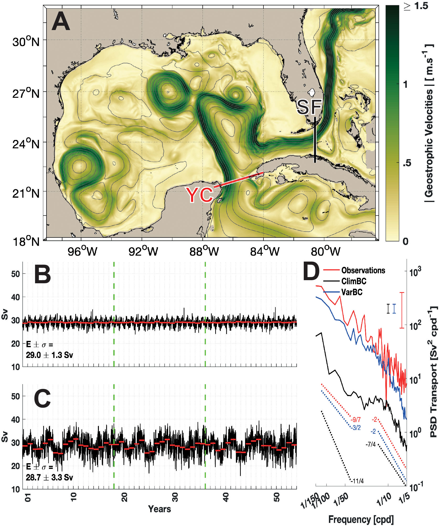
Figure 1 (A) Geographic area of the simulation showing the SSH isolines (SSH increment of 10 cm) and speed (background color) on the first day of the VarBC simulation. The Yucatan Channel (YC) and Straits of Florida (SF) are indicated by red and black sections, respectively, in the upper panel. Transport through the YC in ClimBC (B) and VarBC (C) simulations. Each red line in panels b and c indicates the annual averages, and the green vertical dashed lines separate the three integration cycles. In panels (B, C), the total average (E) and associated standard deviation (σ) are indicated. (D) Power spectral density of transport across the YC in the 54-year simulations (ClimBC in black and VarBC in blue) and over 4 years of CANEK (Athié et al., 2015; Sheinbaum et al., 2016; Candela et al., 2019; Athié et al., 2020) mooring measurements (red). Vertical bars indicate the 95% confidence intervals and dashed lines are the slopes for each dataset.
The two configurations analyzed in this paper are identical, except that one has monthly climatological boundary fields at the open boundaries (hereafter ClimBC) and the other has boundary conditions with daily variability (VarBC). In the ClimBC simulation, the boundary conditions are derived from a bi-weekly climatology produced by four years (2000-2003) of a HYCOM Atlantic free-running (non-assimilative) simulation at 1/12th; therefore, the fields imposed at the lateral boundaries have no interannual nor daily variability and reproduce the seasonal cycle only (Dukhovskoy et al., 2015). The boundary conditions for the VarBC experiment are derived from the ClimBC open boundary conditions by adding T, S, U daily anomalies to the time-averaged T, S, U fields of ClimBC as follows:
Where Tclm is the temperature from the climatology and Trnl from the reanalysis and where — indicate a temporal mean. The daily anomalies are derived from the 0.08∘ HYCOM reanalysis (19.0 and 19.1) for the period 1993-2010 (Chassignet et al., 2009; Metzger et al., 2014).
Both simulations are integrated for 54 years by repeating three times 18 years of atmospheric forcing derived from the CFSR hourly fields as detailed in Dukhovskoy et al. (2015). The ends of the 18-year forcing time series are blended by temporal interpolation of the last three days towards the forcing fields on the first day in order to avoid jumps in the forcing fields between the 18-year cycles. The ocean fields are integrated continuously during these 54 years.
Different time scales at the BCs result in notable variability of the YC transports in the ClimBC and VarBC simulations (1b and c). In the VarBC experiment, one can clearly see the 18-year repeat cycle due to the recycled ocean boundary conditions every 18 years as well as the high and low frequency variability not present in ClimBC. The estimates of the YC transport (mean ± σ) derived from the two simulations (29 ± 1.3 Sv and 28.7 ± 3.3 Sv) are only slightly higher than the transport (27.5 ± 11.3 Sv) computed from roughly 4 years (July 10 2012 to August 07 2016) of CANEK mooring data (Athié et al., 2015; Sheinbaum et al., 2016; Candela et al., 2019; Athié et al., 2020). The 4-year observation-derived transport is within the range of the mean transport estimates from the simulations (note that the observed transport standard deviation includes tides that are not present in the numerical simulations). To illustrate how a 4-year transport estimate can vary over a 54-year time period, the Yucatan transport was computed from 4-year overlapping segments shifted by 1 year over all 54 years of the VarBC experiment. We found that in about 25% of these segments the 4-year modeled YC transport estimates were below the observed 4-year transport of 27.5 Sv. To quantify the impact of adding higher frequency variability, we computed the power spectral density (PSD) of the transport for the two simulations and for the CANEK data (Figure 1D). To smooth the signal, multiple PSD are computed over temporal blocks of 365 days with 50% overlap and averaged to obtain confidence intervals following Thomson & Emery (2014). We focus on the frequency band that is well resolved by the 4-year period of observations. VarBC exhibits a lower PSD than the observations, but the overall shape is similar. The ClimBC PSD, on the other hand is much lower and has a significantly different shape for lower frequencies with a sharp decrease in the PSD slope in the frequency band between about 1/150 and 1/50 cpd that is smoother in VarBC or the observations. Therefore, with more realistic variability of the BCs, the transport variability has more energy for a wide frequency band ranging from interannual variability (Figures 1B, C) to higher frequency such as daily and weekly variability (Figure 1D).
2.2 Satellite altimetry data
In order to compare the model fields of elevation and velocity to observations, Absolute Dynamic Topography (ADT) maps, derived from satellite altimetry, were analyzed. 1/4∘ SSH and the associated surface geostrophic velocities are extracted for the Gulf of Mexico for 26 years (from 01/01/1993 to 31/12/2018) from the global daily multi-mission altimeters DUACS DT2014 (Pujol et al., 2016). These 1/4∘ fields, built from an optimal spatial and temporal interpolation of along-track data, are made available by the European maritime service Copernicus (www.marine.copernicus.eu). Because of the interpolation, the effective spatial resolution is coarser than 1/4∘ and is on the order of a 150-250 km wavelength in the Atlantic Ocean at the latitude of the GoM (Ballarotta et al., 2019). Following Chelton et al. (2019; 2011) who showed that eddy characteristic can be estimated as around 25% of the wavelength, we could expect to resolve an eddy radius of 40-60 km. Thus, the 1/4∘ fields have sufficient spatial resolution to permit the investigation of the mesoscale dynamics of the LC and LCEs which have a typical radius of more than 100 km (e.g., Leben, 2005).
2.3 LC/LCE tracking
In order to compare the dynamics of the LC and LCE in model simulations and observational datasets, one requires an objective definition of the LC/LCE front independent of the dataset being analyzed. Two new objective methods inspired by eddy detection algorithms were developed to automatically track the LC front and identify LCE separation events.
2.3.1 Detection of the Loop Current front
One of the commonly used definitions of the LC front is based on some threshold value of demeaned SSH field such that the contour continuously tracks the LC from the YC to the Straits of Florida [e.g., a threshold of 0.17 m was used in Leben (2005) and Dukhovskoy et al. (2015)]. This definition is, however, sensitive to the choice of the SSH contour and may result in different LC front position and shape as well as differences in the LCE shedding events for different SSH contours. An alternative definition of the LC front, proposed here, tracks the streamline, associated with maximum geostrophic velociy magnitude, that connects the YC to the SF (respectively the red and black lines in Figure 1A). This method, which is hereafter referred to as the <V> method, is described and validated in the Supplementary Material. It assumes that the LC current is mostly in geostrophic balance (e.g., Leben, 2005; Lindo-Atichati et al., 2013; Dukhovskoy et al., 2015) and that the outer limit of the LC is in the vicinity of the core of the jet (e.g., Lindo-Atichati et al., 2013; Dukhovskoy et al., 2015; Hirschi et al., 2019).
2.3.2 Identification of Loop Current Eddy separation events
Most automated methods identify a LC eddy separation as a jump in the length of the LC front. We developed a new method based on the detection of the dynamic structure associated with closed contours of SSH by taking advantage of recent thresholdfree eddy detection algorithms that take into account both merging and splitting events (e.g., Laxenaire et al., 2018; Le Vu et al., 2018). We track the position of anticyclonic recirculation within the LC (e.g., Molinari et al., 1977; Lewis & Kirwan, 1987; Hall & Leben, 2016) identified as an eddy by such algorithms. This recirculation is tracked over time allowing the identification of an eddy separation event as the date at which this recirculation becomes an isolated eddy in the GoM. During the eddy separation event, the trajectory linking the center of the recirculation and of the LCE crosses the LC as the LC front retracts. With this method, one can keep track of detachment and reattachment events and it is therefore possible to identify when a LCE reattaches to the LC without having to set a priori a temporal threshold, nor needing an operator as in Leben (2005). The effectiveness of the method, which uses the TOEddies eddy detection algorithm (Chaigneau et al., 2011; Pegliasco et al., 2015; Laxenaire et al., 2018), was evaluated by comparing the ring separation event dates to the ones obtained by Hall & Leben (2016) using the 17 cm contour method of Leben (2005). In the period from 1 January 1993 to 11 September 2015, 36 events are identified by TOEddies and 32 by Hall & Leben (2016). The 4 additional events identified by TOEddies are among the smallest and least durable with an average LCE radius of 44 km and a lifetime after LC separation of 75 days (the average radius is 115 km with an average lifetime of 285 days).
Overall, these two procedures [Leben (2005) and TOEddies] give very similar results for large LCEs with the only difference being that the TOEddies method, being threshold-free, can detect smaller LCE ejections not identified by the method of Leben (2005).
3 Results
3.1 Comparison of LC and LCE metrics
In this subsection, we summarize metrics for the Loop current derived from the two multi-decadal HYCOM experiments and the altimetry maps to document the impact of the boundary conditions. The metrics are: LC length, LCE shedding period, LCE radius, and duration of the retracted phases. The metrics are computed over the last two cycles only (36 years), with the first cycle considered as an adjustment period.
3.1.1 LC statistics
The length of the LC front is a traditional measure of its extension in the GoM (Hirschi et al., 2019). Indeed, Leben (2005) has shown that its length is strongly correlated with many other variables such as its surface area, volume, and maximum longitudinal and latitudinal extensions. The length of the LC (∮dl), computed using the method described in 2.3.1, is normalized by the beeline distance (BD) between the positions of the front (Figure 2) in the YC and the SF (Equation 2).
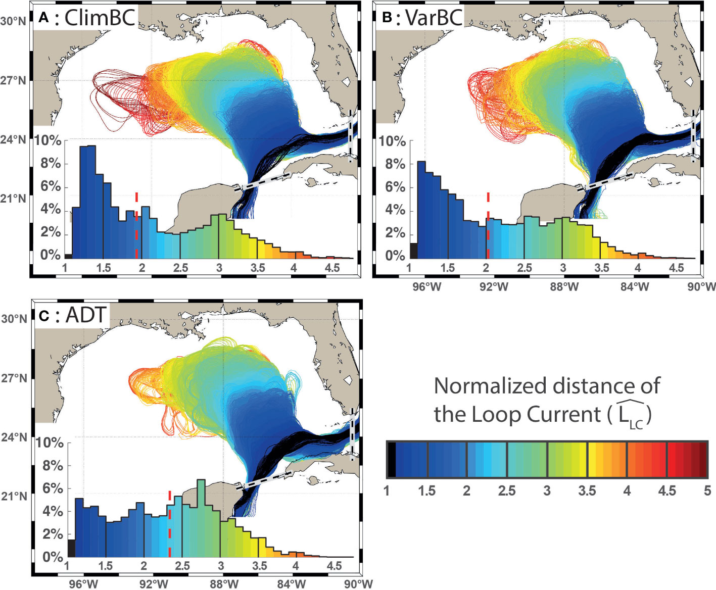
Figure 2 Shape of the LC for the last two cycles of ClimBC and VarBC (A, B) and of the ADT (C). The histogram of LLC distribution (percentage) is displayed in the lower left corner of each panel. The color represents the normalized LLC length both in maps and histograms as described in the lower right panel of this figure. .
The geographic position and histograms of LLC for the three datasets are plotted in Figure 2. Overall, the mean shape of the Loop Current is very similar in the three datasets for LLC < 3.5 (blue, green and yellow contours), which is about 90% of the time. The mean and the median LLC are close, ranging from 1.9 to 2.3, with slightly higher values in the ADT maps. However, the histograms (Figure 2) show that the most frequent value for LLC is 2.8 in the altimeter maps versus 1.4 and 1.2 in ClimBC and VarBC, respectively. Thus, in the simulations, the LC spends more time in a retracted phase (i.e. low LLC) than in the altimetry. In all cases, there is a bimodal distribution, but the first mode (low LC value) is much more pronounced in the simulations. As surmised, the LLC is highly correlated with the LC surface area with a correlation coefficient (R) greater than 0.98.
Furthermore, Figure 2 demonstrates that the LC extends further west in ClimBC than in VarBC. This is confirmed by the normalized histograms for the western and northern extensions of the LC displayed in Figure 3 (grey for ClimBC and cyan for VarBC). Overall, the two distributions are close to each other, but as already pointed out by Dukhovskoy et al. (2015) for ClimBC, while the distributions of the maximum western longitude of the LC have similar statistics to the altimeter-derived data, the distribution of the maximum northern latitude is more strongly bimodal in the model simulations than in the data.
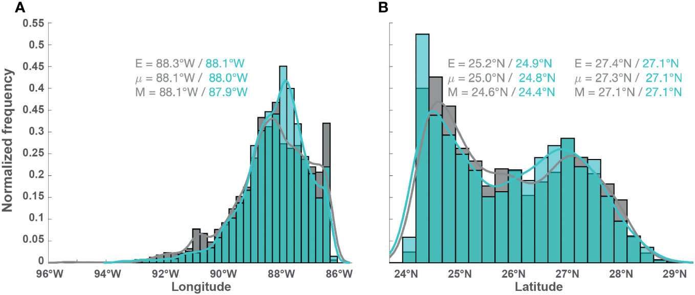
Figure 3 Normalized histograms (bars) and associated kernel density estimates (solid lines) of the Loop Current (LC) western extension (A) and northern extension (B) with 1/4∘ binning derived from the last two cycles of ClimBC (grey) and VarBC (cyan). The statistics of each mode of the bimodal distribution of the northern extension are provided. The estimates of the mean (E), median (μ), and mode (M) are shown in all the panels.The plain lines indicate the kernel probability density estimates (Rice, 1995). .
3.1.2 LCE statistics
The LCE statistics are presented in terms of number of shedding events per year, eddy separation period, and eddy radius in Table 1. In the ClimBC simulation, very long eddy separation intervals occur substantially more often than in the observations or in the VarBC simulation. In 20% of the cases, the separation period exceeds 18 months in ClimBC compared to only a few percent both in the VarBC experiment and in the altimetry. The number of LCEs per year ranges from 1.2 to 1.6, giving an average eddy separation period of 7.3 to 9.4 months. This range encompasses the mean period of 8 months (243.3 days) obtained by Hall & Leben (2016) from CCAR data over the first 20 years of altimetry measurements. The shortest eddy separation period is in the ADT fields (7.3 months) and the longest is in the ClimBC simulation (9.4 months). The differences are not significant when compared to the 95% confidence interval (CI) ranging from 1.6 to 2.9 months, but the VarBC eddy separation period is closer to the ADT fields than ClimBC. In terms of eddy size, the HYCOM simulations generate LCEs with a mean radius slightly larger than in the altimeter fields, but the differences are not significant. However, the LCE with radii smaller than 100 km represent a larger portion of the ADT eddies than for the simulations. The difference is less pronounced for the larger eddies with radius greater than 150 km.
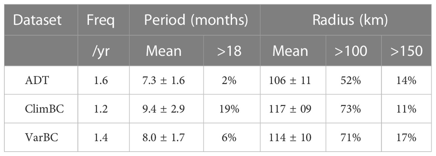
Table 1 Frequency, eddy shedding period, and LCE radii for ADT, ClimBC, and VarBC.
3.1.3 Retracted phases
The retracted phases, i.e., the periods when the LC does not penetrate inside the GoM are identified as events where the LLC remains below 2.3 (i.e., largest average LLC computed from the three datasets) for at least 4 months [i.e. about half of the average eddy separation period; see Table 1 and Hall & Leben (2016)]. The 4-month minimum in the retracted phase effectively filters out cases when the transient decrease of LLC is followed by a sharp increase in the case of the detachment and reattachment of a LCE. This is illustrated in Figure 4 where the LCE separations and retracted phases are identified in the time series of LLC for the three datasets. The average LLC for the retracted phases is 1.5.
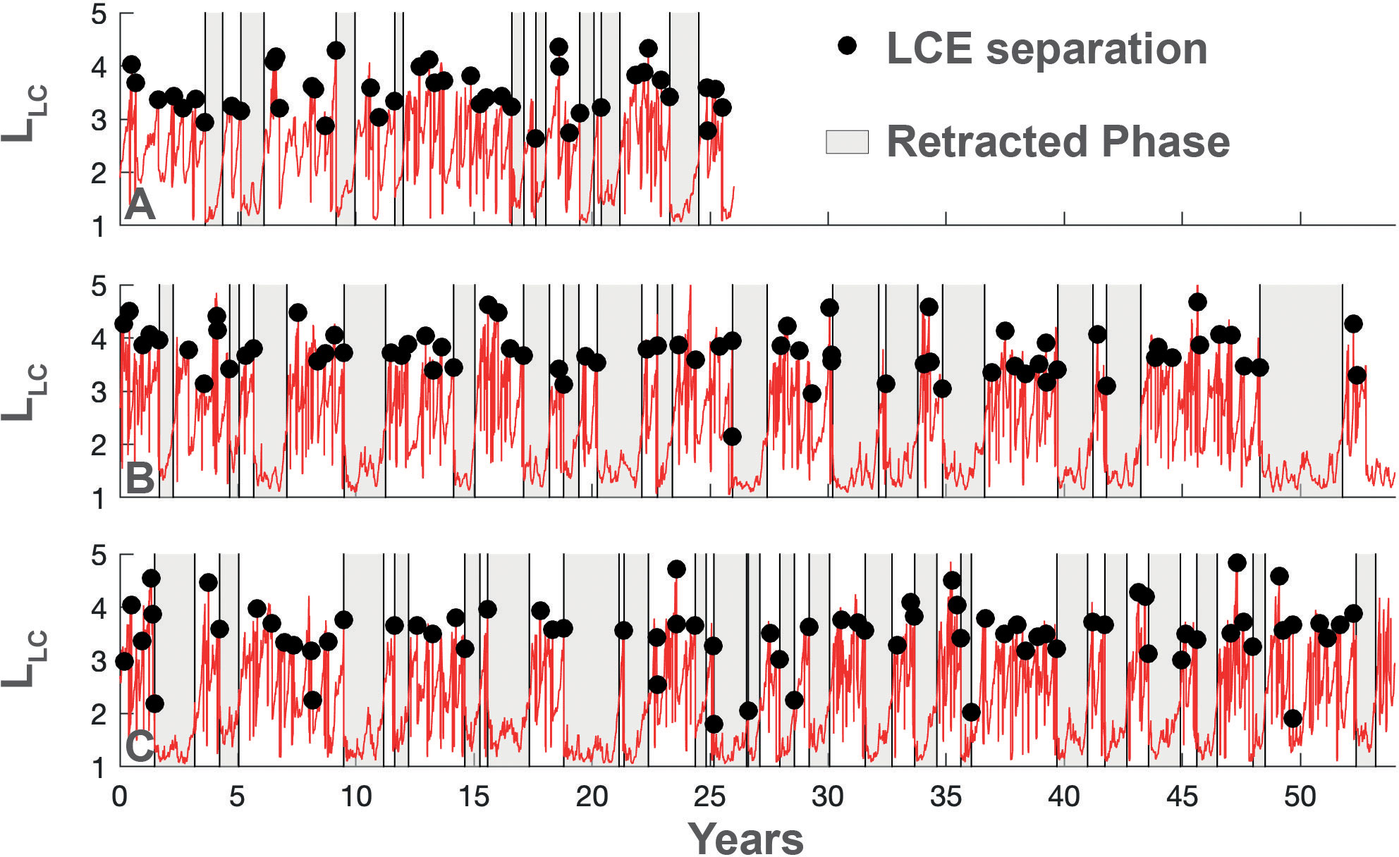
Figure 4 Time series of LLC, separation of LCE and retracted phases in ADT (A), ClimBC (B) and VarBC (C). In b and c, the fist cycle of 18 years is not analyzed in this section.
The statistics for the retracted phases are given in Table 2. The frequency of these events is quite similar among the datasets. However, if we consider the percentage of time that the LC is in a retracted phase, the modeled LC spends more time in a retracted phase than in the observed ADT fields. The differences are quite significant since the LC is in a retracted position about 25% of the time in the ADT fields while it is more than 40% in the simulations. The average duration for the retracted phase is longest in the ClimBC experiment (19.4 versus 11.6 for VarBC and 8.6 months for ADT). The duration of the retracted phases is significantly different in ClimBC at the 95% level using a Kolmogorov-Smirnov test with two samples (Massey, 1951).
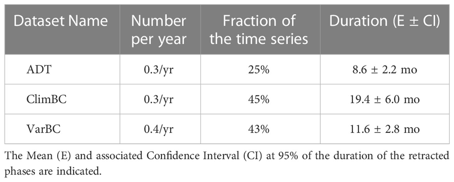
Table 2 Number per year, fraction of the time series and duration of the retracted phases for the three data sets (last two cycles for ClimBC and VarBC).
3.2 Relation between LC properties and flow across the YC
In this subsection, the characteristics of the Yucatan Current (surface velocity, vertical flow structure) during the LC expansion and retracted phases are analyzed.
3.2.1 Flow properties during retracted phase
The YC flow characteristics during the LC retracted are compared to the properties during the month following their end when the LC expands in ClimBC (Figure 5) and VarBC (Figure 6) experiments. The meridional velocities across the YC are extracted (Panel A in Figures 5, 6) and the percentages of time spent in a specific cell by a velocity range versus longitude are computed separately for the two periods of interest, i.e., during the retracted phase and for the month after its end (Panels b and c in Figures 5, 6). In both simulations, there is a clear difference in the mean velocity profile between the two periods with a higher maximum velocity shifted to the west in the periods after the retracted phases when the LC starts to invade the GoM. The variability of the velocity profile is higher during the retracted phases, possibly because of the higher number of days used to compute the percentages, but also because the Loop current position is not steady when in retracted position as it can be seen in Figure 4. The difference in variability between ClimBC and VarBC is especially noticeable when comparing the panels b to d in Figures 5, 6. The variability is substantially smaller in ClimBC in the months following the retracted periods.
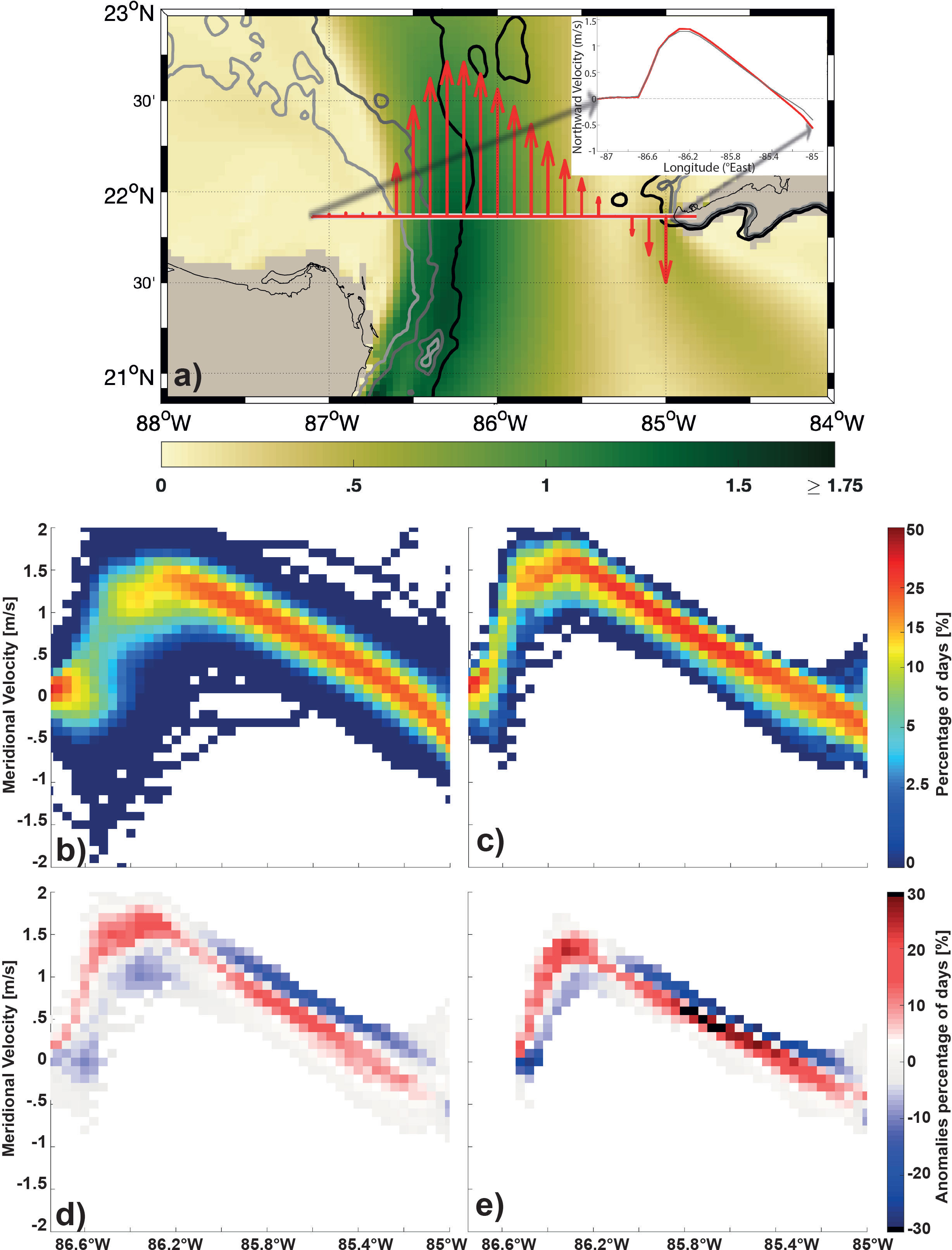
Figure 5 (A) Time averaged surface meridional velocity across the YC from the Campeche Bank to Cuba in ClimBC. Distribution of the time averaged surface meridional velocity along the section in ClimBC is drawn in red in the upper right corner of the panel and the one of VarBC is in grey (B) Occurrence (percentage of time) of meridional velocity (vertical axis) along the YC section (longitudes along the section are on X axis) during the LC retracted phase and (C) during the first month of the LC extension phase; Occurence of meridional velocity distribution during retracted phase minus that of the month following their end (vertical axis) along the YC section (longitudes along the section are on X axis) at the surface (D) and at 100 m (E).
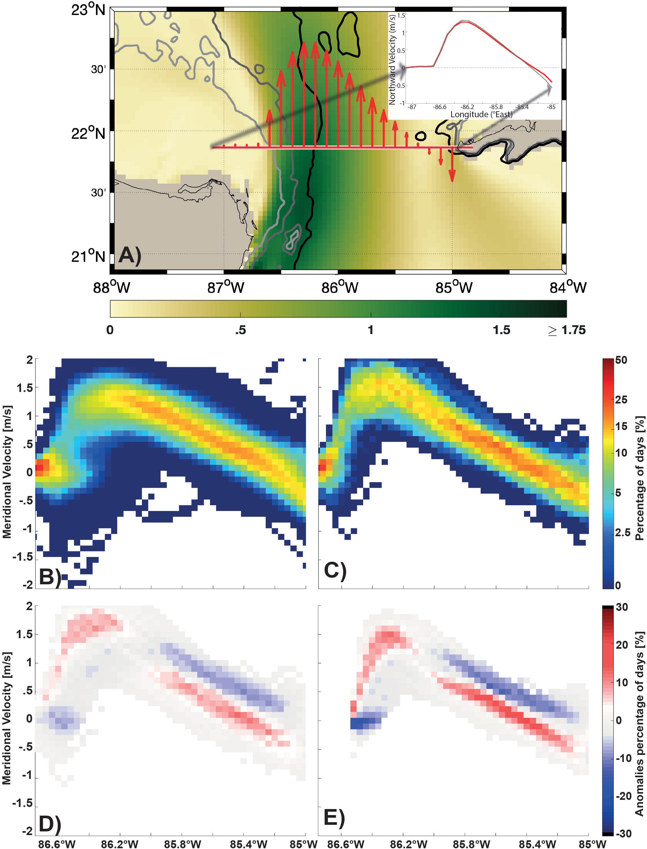
Figure 6 Same as in Figure 5 for VarBC, except that the distribution of the time averaged surface meridional velocity along the section in VarBC is drawn in red in the upper right corner of the panel and the one of ClimBC is in grey.
To compare the surface meridional velocity distribution along the YC section between these two phases, anomalies are constructed by subtracting Panel B from Panel C (Panel D in Figures 5, 6). The position of the current found more often during the extension phase than during the retracted phase is in red and the opposite is blue. After a retracted phase, the average velocity profile has a higher maximum velocity and the surface meridional velocity distribution is shifted to the west. It is the same at 100 m (Panel E in Figures 5, 6), but with less variability, indicating that the surface signature extends at depth. Note that the results are very similar between ClimBC and VarBC, except that there is a larger spread in the differences in VarBC than in ClimBC because of the higher variability prescribed at the boundaries.
In order to quantify the differences between and after the retracted phases, the daily surface velocity profiles are used to calculate a) the value and position of the maximum velocity (Vmax and XVmax), b) the vorticity west and east of this maximum (Vort West and East), as well as c) the cumulative east-west surface velocity over 1 m (1D Transport). Vorticity is computed using the first half of the velocity slopes near the maximum speed to capture the core of the LC jet. Figure 7 displays all these different variables in one diagram for the surface. The distribution of values during the two periods (retracted phases and after retracted phases) can then be compared to each other. For example, the median of the Vmax distribution at the surface after retracted phases is higher than the ∼ 65th percentile of the complete time series (75th percentile in ClimBC and 68th percentile in VarBC). By contrast, this value is slightly less than the 40th percentile during retracted phases. Further examination of these diagrams show that the periods of retracted phases are associated with a) low values of Vmax, b) a position of the main LC core shifted to the east, and c) a lower cyclonicity (anticyclonicity) west (east) of the LC core. There is no noticable difference in surface transport (1D Transport). Once the retracted phases end, there is a shift in these variables to a) high values of Vmax, b) a position of the main LC core shifted to the west, and c) higher cyclonicity (anticyclonicity) west (east) of the LC core. The same method was applied to the velocity field at 100 m resulting in a very similar behavior suggesting that it is not a process limited to the surface.
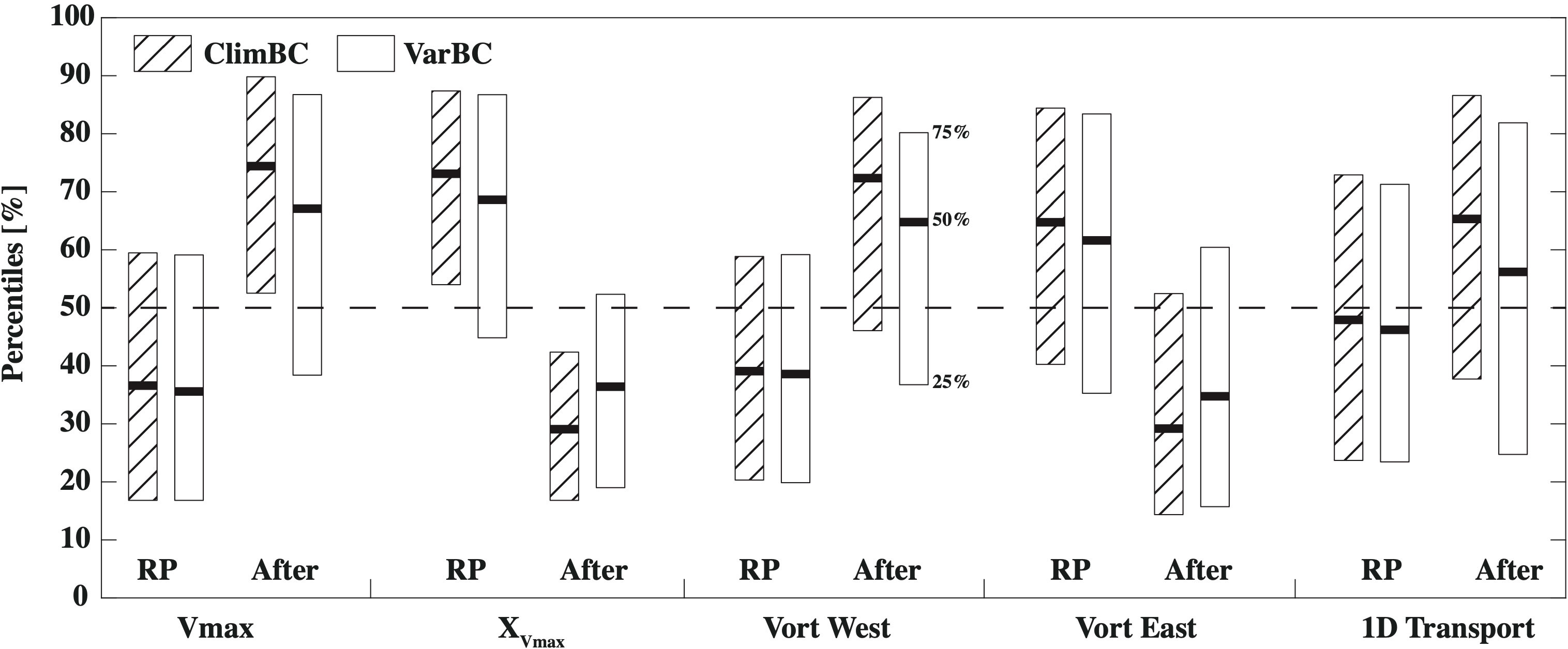
Figure 7 The box diagrams showing the median (thick black line) and the interquartile range (the top and bottom lines of the boxes) for: the maximum surface meridional velocity along the section shown in Figure 5A; position of the maximum velocity (Vmax and XVmax) along this section; the vorticity west and east of this maximum (Vort West and East) and of the cumulative surface velocity over 1 m (1D Transport) at the surface relative to the total time series (percentiles in the vertical axis) during the retracted phases (RP) and the month following the end of these phases (After). Note that XVmax is increasing toward the East. Hatched boxplots represent ClimBC and clear boxes represent VarBC.
3.2.2 Link between flow properties and evolution of the LC area
In the previous section, the relationship between the retracted and extending states of the LC system and the flow through the YC was analyzed. In this section, we make an attempt to generalize these results by extending the analysis to periods when the LC is in the extended phase and invades the GoM and when it retracts shrinking in size. These phases are identified as in Nedbor-Gross et al. (2014) by calculating the time derivative of the LC surface (dtA) at time t by subtracting the mean area of the previous 10 days from the mean area of the next 10 days (20-day time interval). dtA>0 implies expansion and dtA<0 retraction.
The anomalies of the Yucatan flow properties from the time averaged fields as functions of the sign of dtA are shown in Figure 8 for ClimBC and in Figure 9 for VarBC. The first three rows of each figure highlight the changes in hydrographic properties (temperature, salinity, density) of the flow across the YC with respect to the sign of dtA. These figures show that the westward shift of the LC core leading to the expansion of the LC is, in the center of the YC, associated with warmer and saltier water than the temporal mean. It results in lighter water entering the GoM in the center of the section whereas the opposite occurs at its lateral boundaries and close to the surface.
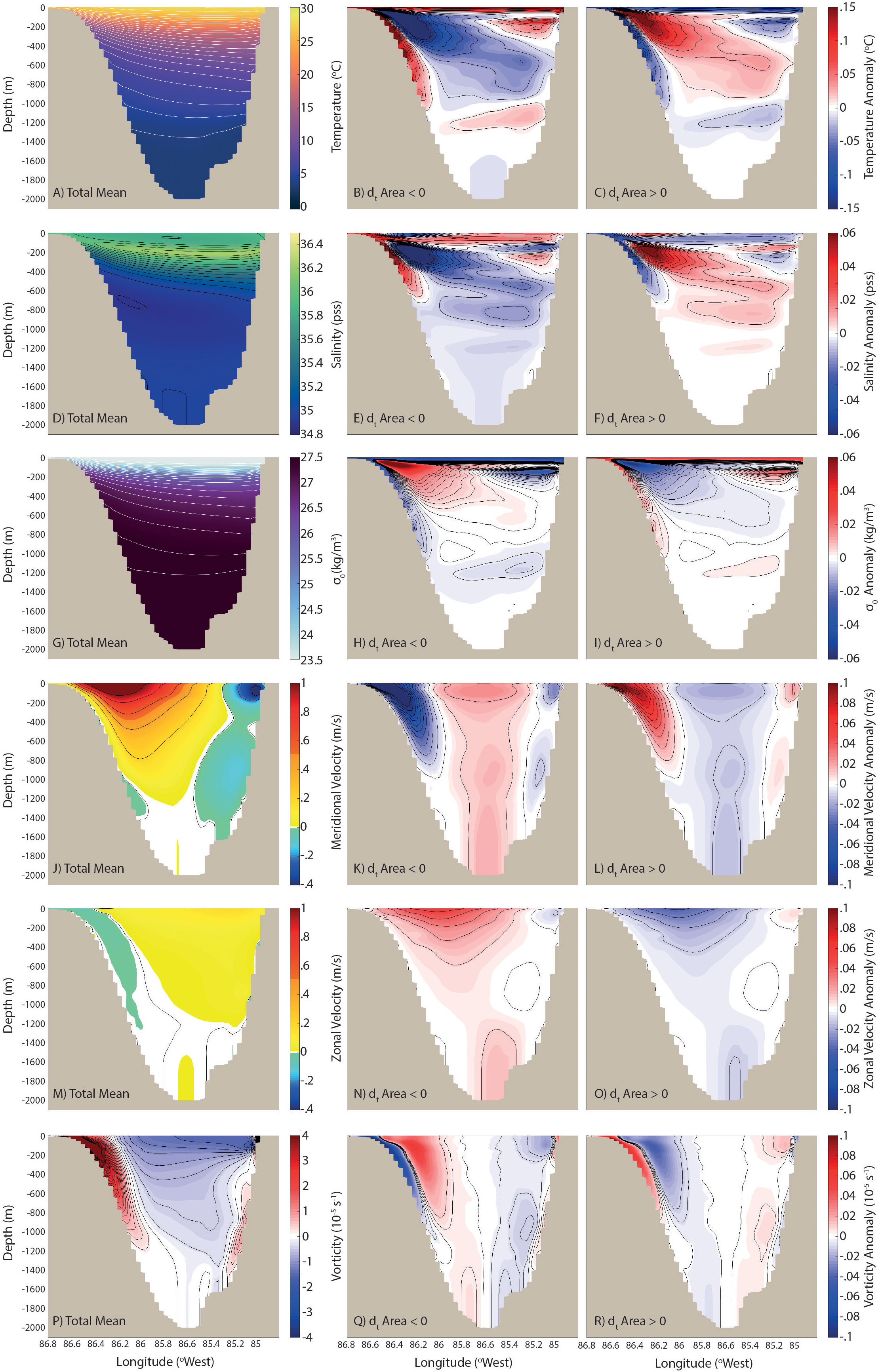
Figure 8 From the first to the last row, the fields of temperature, salinity, density, meridional, zonal velocities and vorticity respectively through the YC in the ClimBC simulation. The complete mean fields of these variables are shown in the first column and the associated mean anomalies when the LC “shrinks” and “grows” across the GoM are provided in the second and third columns respectively.
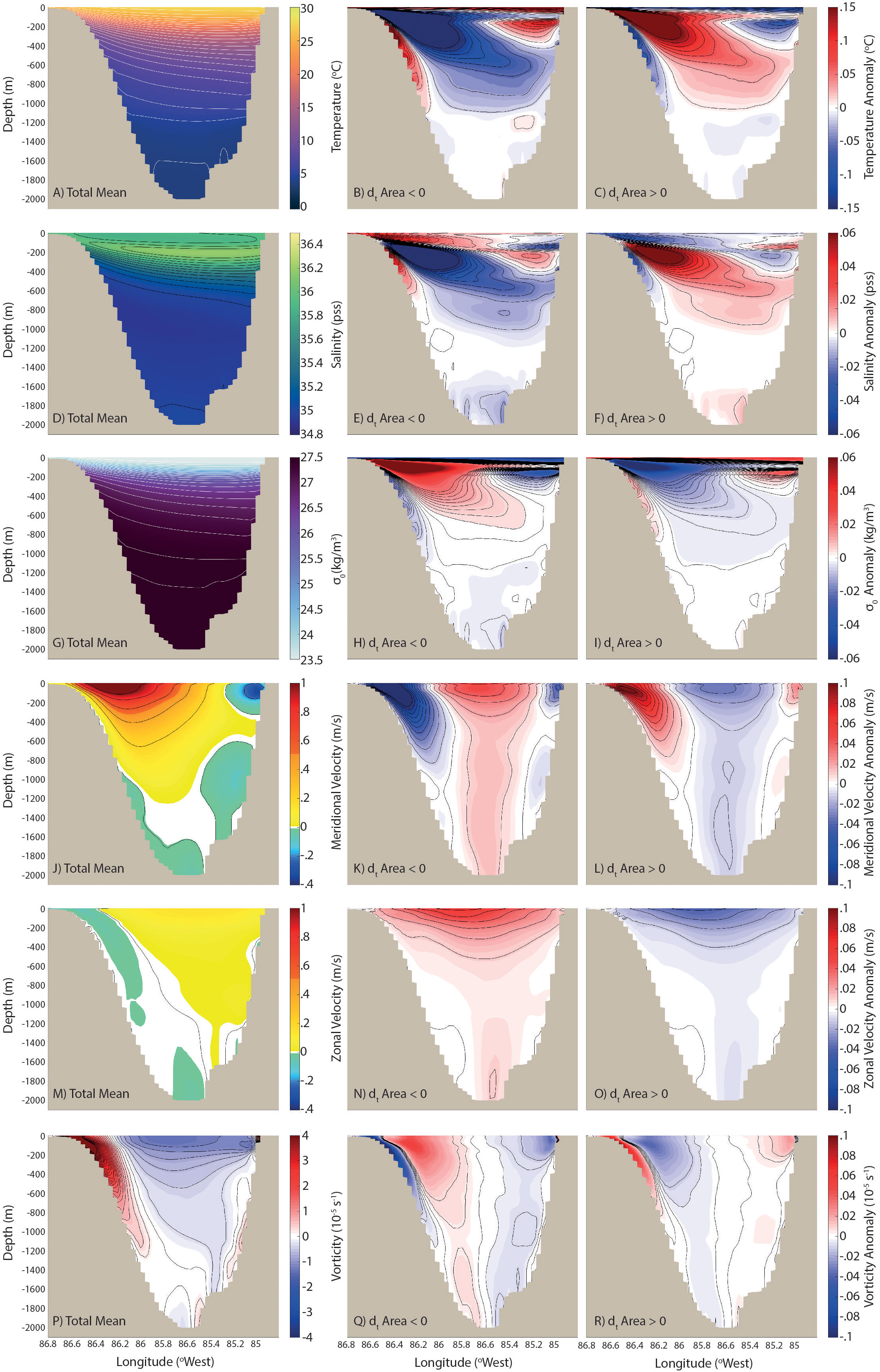
Figure 9 Same as Figure 8 for VarBC.
The westward drift and higher intensity of the maximum of the meridional velocity in the LC jet when it invades the GoM, identified in the previous subsection, can be seen in panels J to L of Figures 8, 9. The zonal displacement of the maximum velocity is quite strong in the upper 1000 m, especially close to the western boundary, with a higher transport in the upper layer (Table 3). In the center of the current, meridional velocity anomalies are negative throughout the complete water column during expansion, which generates in the lower layer an outward flow (Table 3) as extensively discussed by different authors (Maul, 1977; Bunge et al., 2002; Ezer et al., 2003; Lee & Mellor, 2003; Chang & Oey, 2011; Nedbor-Gross et al., 2014). This is true for both ClimBc and VarBC (see summary in Table 3). The changes in the zonal component of the current through the YC (Panels M to O) indicate that, when the LC invades the GoM, the velocity core is shifted to the northwest (northeast when the LC retracts). Finally, as pointed out in the previous subsection, the displacement of the main core of the jet and its intensification lead to higher anticyclonic shear to the east of the LC and higher cyclonic shear to the west. The detachment of the main core along the island of Cuba during the “growth” of the LC leads to small areas of positive vorticity that are visible in the eastern part of the channel. Overall, the results obtained by comparing particular phases of the LC clearly illustrates how the flow properties across the YC change when the LC invades the GoM as opposed to when it retracts.
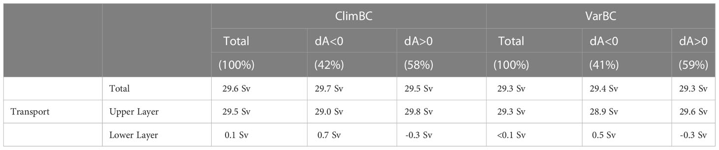
Table 3 Average transport through the YC. The mean values are calculated either using the full period or both periods with a different sign of the time derivation of the LC area in the GoM (dtA). The lower layer is identified as HYCOM layers below which the time averaged transport is close to zero.
3.2.3 Eddies in the Yucatan channel and the Loop Current
As discussed by many authors (e.g., Murphy et al., 1999; Candela et al., 2002; Oey et al., 2003; Athié et al., 2012; Androulidakis et al., 2021), the properties of the LC can be modulated by the entry of coherent patches of vorticity into the GoM. In this subsection, we characterize and quantify the eddies entering the GoM by applying the TOEddies algorithm of Laxenaire et al. (2018) on the SSH contours (Table 4). The eddies are separated into two categories when they enter the Gulf of Mexico via the Yucatan Channel, either west or east of the maximum mean surface velocity (see the velocity distribution across the Yucatan Channel in Figures 5, 6). We find that all the anticyclones enter the GoM east of maximum velocity and that there are more anticyclones entering the GoM during the LC extension vs the LC retraction. On the other hand, we find that there are more cyclones entering the GoM west of maximum velocity when the LC is retracting and more entering to the east when the LC is growing. Most of those cyclones enter to the east of the maximum velocity enter near Cuba, providing a positive vorticity influx. There are significant differences between the two simulations with about 3 times more anticyclones entering the GoM in VarBC than in ClimBC; but both simulations have approximately the same number of cyclones. This indicates that cyclones are more likely to be formed locally south of Cuba while anticyclones are more likely to be injected in the model domain via the open boundary conditions.
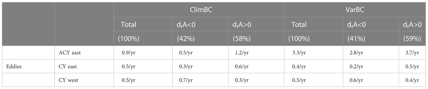
Table 4 Number of eddies entering the GoM through the YC. The mean values are calculated either using the full period or both periods with a different sign of the time derivation of the LC area in the GoM (dtA). Anticyclones (ACY) and cyclones (CY) are studied separately depending on whether they cross the YC west of the maximum velocity or east.
Androulidakis et al. (2021) named the anticyclones south of the Yucatan Channel, CARibbean Anticyclones (CARAs), and, as in their study, we note that when the LC retracts, a large CARA is often found south of the LC while one anticyclone is often found south of Cuba when the LC expands (not shown). Here, we go one step further by documenting the origin and fate of these eddies. To do this, we track the eddies entering the area depicted by a polygon (in gray in Figure 10). Figure 10 shows that the CARAs originate mainly from two distinct areas, Caribbean Sea (black trajectories) and an area between the northwestern tip of the main island of Cuba and the Isle of Youth (blue trajectories). Most of the anticyclones exit north into the GoM (green trajectories), but a small portion recirculates within the Caribbean Sea (black trajectories). In both simulations, there are more anticyclonic eddies entering the polygon than exiting which indicates that merging events occur prior to entering the GoM. As already stated, there are more anticyclonic eddies entering the GoM in VarBC than in ClimBC since eddies can enter the southern boundary in VarBC via the open boundary conditions. We do find that anticyclonic eddies entering the GoM are somewhat linked to an increase in the LC area as shown in Table 4, but overall there is no obvious correlation between the LC dynamics and the eddies entering or exiting the GoM. However, it is worth noting that, from the blue trajectories in Figure 10, more eddies appear to drift from east to west (entering) that the inverse (exiting) the polygon, suggesting that the CARAs upstream of the GoM discussed by Androulidakis et al. (2021) mainly leave this area to enter the GoM.
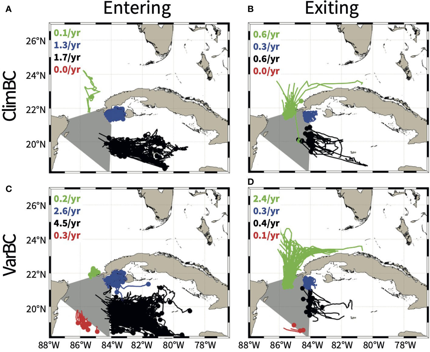
Figure 10 Origin (Entering, A, C) and termination (Exciting, B, D) of the Caribbean Anticyclones in ClimBC (A, B) and VarBC (C, D). The eddies are separated if they enter/exit the area of interest by north (green), east (blue), south (black) and west (red) routes. The numbers in the upper left corner of each panel indicate the number of structures per year, with the color indicating the route followed.
4 Discussion and summary
In this study, we document the impact of boundary conditions (BC) on the the Loop Current (LC) evolution and associated LC eddy (LCE) formation. The importance of inflow variability on the LC retracted and extended phases is demonstrated by comparing two multi-decadal GoM simulations, identical except for their open boundary conditions (climatological versus variable). We show that the addition of daily interannual variability does eliminate the unrealistically long period of LC retracted phases found in the climatological simulations (Dukhovskoy et al., 2015).
To unveil the processes explaining the differences between the numerical simulations, a detailed study of the structure of flows entering the Gulf of Mexico through the Yucatan Channel is performed. It shows that the LC tends to extend into the GoM when the flow across the YC satisfies the following conditions when compared to the mean state:
● Maximum velocity shifted westward, directed toward the north-west and of higher magnitude, leading to higher horizontal shear and vorticity on both side of the jet.
● Stronger vertical shear close to the surface and weaker subsurface between 200 and 800 m.
● Higher transport toward the GoM in the upper layer of the YC compensated by transport toward the Caribbean in the lower layers.
● Higher number of mesoscale eddies entering in the GoM (both polarity) in the main core of the LC, but with a lower number of cyclones in the vicinity of the Mexican coast. A larger number of anticyclonic eddies is also found to enter the GoM when the LC area increases.
The link between the westward displacement of the LC velocity core and change of LC area in the GoM was first documented by Nedbor-Gross et al. (2014) following the work of Athié et al. (2012) who identified such displacement in relation to LCE shedding. When investigating the relationship between the LC area and the time integration of the deep YC transport, Nedbor-Gross et al. (2014) showed that, when the LC area is larger than its 75th percentile, the YC transport profile shifts west and that, when the LC area is below the 25th percentile, the YC transport profile shifts east and broadens. The Nedbor-Gross et al. (2014) results are in agreement with the results presented in this paper as well as those of Androulidakis et al. (2021). One can therefore envision that assimilation of the Yucatan Channel velocity profile could lead to substantial improvements in the forecasting of the Loop Current evolution.
Furthermore, Candela et al. (2002) and Oey (2004) surmise that an influx of cyclonic potential vorticity flux anomaly extends the Loop Current and influx of anticyclonic potential vorticity flux anomaly “triggers” a retraction. These vorticity fluxes are controlled by the intensity of the current near the surface at the western portion of the YC where the cyclonic horizontal shear of Ertel’s potential vorticity are maximum (see the the upper right panel of Figure 2 of Oey (2004)). On the other hand, the theory of the momentum imbalance paradox (Pichevin & Nof, 1997; Nof & Pichevin, 2001; Nof, 2005) states that the fraction of the flux transferred to the bulb should increase when the anticyclonicity of the input flux increases (e.g. discussion of parameter α in Nof (2005)). These two results a priori may appear to be contradictory, but they are consistent with our findings which show that an increase in LC maximum velocity not only leads to a higher cyclonicity in the western part of the LC, but also higher anticyclonicity in the core of the eastern part of the LC.
Mesoscale dynamics in the Caribbean Sea upstream of the Loop Current as a possible important factor on Yucatan flow variability and LC dynamics has been discussed in many studies (e.g., Murphy et al., 1999; Candela et al., 2002; Abascal et al., 2003; Oey et al., 2003; Athié et al., 2012; Garcia-Jove et al., 2016; Androulidakis et al., 2021). In particular, Garcia-Jove et al. (2016) showed that Caribbean eddies activity directly impact the LCE separation period, and thus LC dynamics, by suppressing these eddies in numerical simulations via increasing viscosity in the Caribbean Sea. Furthermore, Androulidakis et al. (2021) documented a relation between the presence of CARibbean Anticyclones (CARAs) upstream of the GoM and phases of the LC. They showed that, when a CARA lies south of the YC, the LC tend to be retracted and the inverse is found when it expands. We obtained the same results (not shown) and focused on the fluxes of eddies in the CARAs area. The number of eddies entering in the GoM increases when the LC extends. While the cyclones are formed locally, anticyclonic eddies can originate far from the Caribbean Sea and are thus more numerous in VarBC where they can be formed at the boundary of the domain due to the variable boundary conditions. These results are in agreement with the work of Huang et al. (2021) which demonstrate that anticyclonic eddies in the western tropical Atlantic Ocean can enter the Gulf of Mexico and thus are a direct product of variable boundary conditions.
The choice of the boundary conditions (monthly climatology versus realistic variability added to the climatology) does not have a significant impact on the periodicity of the LC eddy formation, but when interannual daily perturbations are added at the boundaries, the durations of the retracted phases are significantly shorter and better agree with altimetry-derived LC statistics than when using climatological boundary conditions. The added variability impacts the dynamics of the flow across the YC and associated eddies which are strongly linked to the dynamics of the LC and explains the differences found in the simulations. However, with so many different parameters impacting the dynamics of the LC, it is a complicated task to clearly identified a predominant factor. Therefore, while this study of the sensitivity of the LC to the BCs (primarily, the inflow variability) confirmed the importance of the latter, further analysis with other simulations such as with constant BCs or different atmospheric forcings could be studied to reveal other mechanisms acting on the LC dynamics such as, for example, frequency of the LCE shedding.
Data availability statement
The raw data supporting the conclusions of this article will be made available by the authors, without undue reservation.
Author contributions
All authors designed the study. DD and SM ran the numerical simulations. RL performed the data analysis and, with EC, wrote the first version of the article. All the authors contributed to the article and approved the submitted version.
Funding
We acknowledge support from the Gulf Research Program of the National Academies of Sciences, Engineering, and Medicine under award numbers 2000009966 and 2000013149. The content is solely the responsibility of the authors and does not necessarily represent the official views of the Gulf Research Program or the National Academies of Sciences, Engineering, and Medicine. We also acknowledge support from the Office Naval Research (ONR) Grant N00014-19-1-2671
Acknowledgments
The HYCOM simulations were performed on supercomputers at the US Navy DoD Supercomputing Resource Center (DSRC) in Stennis Space Center, Mississippi, using computer time provided by the US DoD High Performance Computing Modernization Program. The gridded altimeter products were produced by SSALTO/DUACS and distributed by the Copernicus Marine Environment Monitoring Service. We acknowledge Dr. Gabriela Athie de Velasco, Dr. Julio Candela and Dr. Julio Sheinbaum who shared the ADCP data from the CANEK program.
Conflict of interest
The authors declare that the research was conducted in the absence of any commercial or financial relationships that could be construed as a potential conflict of interest.
Publisher’s note
All claims expressed in this article are solely those of the authors and do not necessarily represent those of their affiliated organizations, or those of the publisher, the editors and the reviewers. Any product that may be evaluated in this article, or claim that may be made by its manufacturer, is not guaranteed or endorsed by the publisher.
Supplementary material
The Supplementary Material for this article can be found online at: https://www.frontiersin.org/articles/10.3389/fmars.2023.1080779/full#supplementary-material
References
Abascal A., Sheinbaum J., Candela J., Ochoa J., Badan A. (2003). Analysis of flow variability in the Yucatan Channel. J. Geophys. Res. 108, 3381. doi: 10.1029/2003JC001922
Androulidakis Y., Kourafalou V., Le Hénaff M., Kang H., Ntaganou N. (2021). The role of mesoscale dynamics over northwestern Cuba in the loop current evolution in 2010, during the deepwater horizon incident. J. Mar. Sci. Eng. 9, 188. doi: 10.3390/jmse9020188
Androulidakis Y., Kourafalou V., Olascoaga M. J., Beron-Vera F. J., Le Hénaff M., Kang H., et al (2021). Impact of Caribbean anticyclones on Loop Current variability. Ocean dynamics, 71 (9), 935–956. doi: 10.1007/s10236-021-01474-9
Athié G., Candela J., Ochoa J., Sheinbaum J. (2012). Impact of Caribbean cyclones on the detachment of loop current anticyclones. J. Geophys. Res.: Oceans 117, C03018. doi: 10.1029/2011JC007090
Athié G., Sheinbaum J., Candela J., Ochoa J., Pérez-Brunius P., Romero-Arteaga A. (2020). Seasonal variability of the transport through the Yucatan channel from observations. J. Phys. Oceanogr. 50, 343–360. doi: 10.1175/jpo-d-18-0269.1
Athié G., Sheinbaum J., Leben R., Ochoa J., Shannon M. R., Candela J. (2015). Interannual variability in the Yucatan channel flow. Geophys. Res. Lett. 42, 1496–1503. doi: 10.1002/2014GL062674
Ballarotta M., Ubelmann C., Pujol M.-I., Taburet G., Fournier F., Legeais J.-F., et al. (2019). On the resolutions of ocean altimetry maps. Ocean Sci. 15, 1091–1109. doi: 10.5194/os-15-1091-2019
Baringer M. O., Larsen J. C. (2001). Sixteen years of Florida current transport at 27° N. Geophys. Res. Lett. 28, 3179–3182. doi: 10.1029/2001GL013246
Behringer D. W., Molinari R. L., Festa J. F. (1977). The variability of anticyclonic current patterns in the gulf of Mexico. J. Geophys. Res. (1896-1977) 82, 5469–5476. doi: 10.1029/JC082i034p05469
Bleck R. (2002). An oceanic general circulation model framed in hybrid isopycnic-Cartesian coordinates. Ocean Model. 4, 55–88. doi: 10.1016/S1463-5003(01)00012-9
Bunge L., Ochoa J., Badan A., Candela J., Sheinbaum J. (2002). Deep flows in the Yucatan channel and their relation to changes in the loop current extension. J. Geophys. Res.: Oceans 107, 26–1–26–7. doi: 10.1029/2001JC001256
Candela J., Ochoa J., Sheinbaum J., López M., Pérez-Brunius P., Tenreiro M., et al. (2019). The flow through the gulf of Mexico. J. Phys. Oceanogr. 49, 1381–1401. doi: 10.1175/jpo-d-18-0189.1
Candela J., Sheinbaum J., Ochoa J., Badan A., Leben R. (2002). The potential vorticity flux through the Yucatan channel and the loop current in the gulf of Mexico. Geophys. Res. Lett. 29, 16–1–16–4. doi: 10.1029/2002GL015587
Chaigneau A., Marie L. T., Gérard E., Carmen G., Oscar P. (2011). Vertical structure of mesoscale eddies in the eastern south pacific ocean: A composite analysis from altimetry and argo profiling floats. J. Geophys. Res.: Oceans 116, C11025. doi: 10.1029/2011JC007134
Chang Y.-L., Oey L.-Y. (2011). Loop current cycle: Coupled response of the loop current with deep flows. J. Phys. Oceanogr. 41, 458–471. doi: 10.1175/2010jpo4479.1
Chassignet E. P., Hurlburt H. E., Metzger E. J., Smedstad O. M., Cummings J. A., Halliwell G. R., et al. (2009). US GODAE: Global ocean prediction with the HYbrid coordinate ocean model (HYCOM). Oceanography 22, 64–75. doi: 10.5670/oceanog.2009.39
Chassignet E. P., Smith L. T., Halliwell G. R., Bleck R. (2003). North Atlantic simulations with the hybrid coordinate ocean model (HYCOM): Impact of the vertical coordinate choice, reference pressure, and thermobaricity. J. Phys. Oceanogr. 33, 2504–2526. doi: 10.1175/1520-0485(2003)033<2504:naswth>2.0.co;2
Chelton D. B., Schlax M. G., Samelson R. M. (2011). Global observations of nonlinear mesoscale eddies. Prog. Oceanogr. 91, 167–216. doi: 10.1016/j.pocean.2011.01.002
Chelton D. B., Schlax M. G., Samelson R. M., Farrar J. T., Molemaker M. J., McWilliams J. C., et al. (2019). Prospects for future satellite estimation of small-scale variability of ocean surface velocity and vorticity. Prog. Oceanogr. 173, 256–350. doi: 10.1016/j.pocean.2018.10.012
Chérubin L. M., Morel Y., Chassignet E. P. (2006). Loop current ring shedding: The formation of cyclones and the effect of topography. J. Phys. Oceanogr. 36, 569–591. doi: 10.1175/jpo2871.1
Cochrane J. D. (1972). Separation of an anticyclone and subsequent developments in the loop current, (1969). Contributions on the Physical Oceanography of the Gulf of Mexico LRA Capurio, JL Reid Vol. 2 (Texas A&M University Oceanographic Studies), 91–106.
Donohue K., Watts D., Hamilton P., Leben R., Kennelly M., Lugo-Fernández A. (2016). Gulf of Mexico loop current path variability. Dynamics Atmospheres Oceans 76, 174–194. doi: 10.1016/j.dynatmoce.2015.12.003
Dukhovskoy D. S., Leben R. R., Chassignet E. P., Hall C. A., Morey S. L., Nedbor-Gross R. (2015). Characterization of the uncertainty of loop current metrics using a multidecadal numerical simulation and altimeter observations. Deep Sea Res. Part I: Oceanographic Res. Papers 100, 140–158. doi: 10.1016/j.dsr.2015.01.005
Elliott B. A. (1982). Anticyclonic rings in the gulf of Mexico. J. Phys. Oceanogr. 12, 1292–1309. doi: 10.1175/1520-0485(1982)012<1292:aritgo>2.0.co;2
Ezer T., Oey L.-Y., Lee H.-C., Sturges W. (2003). The variability of currents in the Yucatan channel: Analysis of results from a numerical ocean model. J. Geophys. Res.: Oceans 108, 3012. doi: 10.1029/2002JC001509
Garcia-Jove M., Sheinbaum J., Jouanno J. (2016). Sensitivity of loop current metrics and eddy detachments to different model configurations: The impact of topography and Caribbean perturbations. Atmósfera 29, 235–265. doi: 10.20937/ATM.2016.29.03.05
Hall C. A., Leben R. R. (2016). Observational evidence of seasonality in the timing of loop current eddy separation. Dynamics Atmospheres Oceans 76, 240–267. doi: 10.1016/j.dynatmoce.2016.06.002
Hamilton P. (2009). Topographic rossby waves in the gulf of Mexico. Prog. Oceanogr. 82, 1–31. doi: 10.1016/j.pocean.2009.04.019
Hamilton P., Berger T., Singer J., Waddell E., Churchill J., Leben R., et al. (2000). DeSoto canyon eddy intrusion study, final report. volume II (New Orleans, LA: OCS Study MMS 2000-080, US Dept. of the Interior, Minerals Management Service). Tech. rep., Rep.
Hirschi J. J.-M., Frajka-Williams E., Blaker A. T., Sinha B., Coward A., Hyder P., et al. (2019). Loop current variability as trigger of coherent gulf stream transport anomalies. J. Phys. Oceanogr. 49, 2115–2132. doi: 10.1175/jpo-d-18-0236.1
Huang M., Liang X., Zhu Y., Liu Y., Weisberg R. H. (2021). Eddies connect the tropical Atlantic ocean and the gulf of Mexico. Geophys. Res. Lett. 48, e2020GL091277. doi: 10.1029/2020GL091277
Hurlburt H. E., Thompson J. D. (1980). A numerical study of loop current intrusions and eddy shedding. J. Phys. Oceanogr. 10, 1611–1651. doi: 10.1175/1520-0485(1980)010<1611:ansolc>2.0.co;2
Johns W. E., Townsend T. L., Fratantoni D. M., Wilson W. D. (2002). On the Atlantic inflow to the Caribbean Sea. Deep Sea Res. Part I: Oceanographic Res. Papers 49, 211–243. doi: 10.1016/S0967-0637(01)00041-3
Jouanno J., Ochoa J., Pallàs-Sanz E., Sheinbaum J., Andrade-Canto F., Candela J., et al. (2016). Loop current frontal eddies: Formation along the campeche bank and impact of coastally trapped waves. J. Phys. Oceanogr. 46, 3339–3363. doi: 10.1175/jpo-d-16-0052.1
Kara A. B., Rochford P. A., Hurlburt H. E. (2000). Efficient and accurate bulk parameterizations of air—sea fluxes for use in general circulation models. J. Atmospheric Oceanic Technol. 17, 1421–1438. doi: 10.1175/1520-0426(2000)017<1421:EAABPO>2.0.CO;2
Laxenaire R., Speich S., Blanke B., Chaigneau A., Pegliasco C., Stegner A. (2018). Anticyclonic eddies connecting the Western boundaries of Indian and Atlantic oceans. J. Geophys. Res.: Oceans 123, 7651–7677. doi: 10.1029/2018jc014270
Leben R. R. (2005). Altimeter-derived loop current metrics (American Geophysical Union (AGU), Eds. Sturges W. Lugo‐Fernandez A. 181–201. doi: 10.1029/161GM15
Lee H.-C., Mellor G. L. (2003). Numerical simulation of the gulf stream system: The loop current and the deep circulation. J. Geophys. Res.: Oceans 108, 3043. doi: 10.1029/2001JC001074
Leipper D. F. (1970). A sequence of current patterns in the gulf of mexico. J. Geophys. Res. (1896-1977) 75, 637–657. doi: 10.1029/JC075i003p00637
Le Vu B., Stegner A., Arsouze T. (2018). Angular momentum eddy detection and tracking algorithm (AMEDA) and its application to coastal eddy formation. J. Atmospheric Oceanic Technol. 35, 739–762. doi: 10.1175/JTECH-D-17-0010.1
Lewis J. K., Kirwan A. D. Jr. (1987). Genesis of a gulf of Mexico ring as determined from kinematic analyses. J. Geophys. Res.: Oceans 92, 11727–11740. doi: 10.1029/JC092iC11p11727
Lindo-Atichati D., Bringas F., Goni G. (2013). Loop current excursions and ring detachments during 1993-2009. Int. J. Remote Sens. 34, 5042–5053. doi: 10.1080/01431161.2013.787504
Lindo-Atichati D., Bringas F., Goni G., Muhling B., Muller-Karger F., Habtes S. (2012). Varying mesoscale structures influence larval fish distribution in the northern gulf of Mexico. Mar. Ecol. Prog. Ser. 463, 245–257. doi: 10.3354/meps09860
Lugo-Fernández A. (2007). Is the loop current a chaotic oscillator? J. Phys. Oceanogr. 37, 1455–1469. doi: 10.1175/jpo3066.1
Massey ,. F. J. Jr. (1951). The kolmogorov-smirnov test for goodness of fit. J. Am. Stat. Assoc. 46, 68–78. doi: 10.1080/01621459.1951.10500769
Maul G. (1975). An evaluation of the use of the earth resources technology satellite for observing ocean current boundaries in the gulf stream system. Technical Report (Environmental Research Laboratories).
Maul G. A. (1977). The annual cycle of the gulf loop current part i: Observations during a one-year time series. J. Mar. Res. 35, 29–47.
Metzger E. J., Smedstad O. M., Thoppil P. G., Hurlburt H. E., Cummings J. A., Wallcraft A. J., et al. (2014). US Navy operational global ocean and Arctic ice prediction systems. Oceanography 27, 32–43. doi: 10.5670/oceanog.2014.66
Molinari R. L., Baig S., Behringer D. W., Maul G. A., Legeckis R. (1977). Winter intrusions of the loop current. Science 198, 505–507. doi: 10.1126/science.198.4316.505
Moreles E., Zavala-Hidalgo J., Martínez-López B., Ruiz-Angulo A. (2021). Influence of stratification and Yucatan current transport on the loop current eddy shedding process. J. Geophys. Res.: Oceans 126, e2020JC016315. doi: 10.1029/2020JC016315
Murphy S. J., Hurlburt H. E., O’Brien J. J. (1999). The connectivity of eddy variability in the Caribbean Sea, the gulf of Mexico, and the Atlantic ocean. J. Geophys. Res.: Oceans 104, 1431–1453. doi: 10.1029/1998JC900010
Nedbor-Gross R., Dukhovskoy D. S., Bourassa M. A., Morey S. L., Chassignet E. P. (2014). Investigation of the relationship between the Yucatan channel transport and the loop current area in a multidecadal numerical simulation. Mar. Technol. Soc. J. 48, 15–26. doi: 10.4031/MTSJ.48.4.8
Nof D. (2005). The momentum imbalance paradox revisited. J. Phys. Oceanogr. 35, 1928–1939. doi: 10.1175/JPO2772.1
Nof D., Pichevin T. (2001). The ballooning of outflows. J. Phys. Oceanogr. 31, 3045–3058. doi: 10.1175/1520-0485(2001)031<3045:tboo>2.0.co;2
Ntaganou N., Kourafalou V., Beron-Vera F., Olascoaga M., Le Henaff M., Androulidakis I. (2023) Influence of Caribbean eddies on the loop current system evolution. Submitted to Front. Mar. Sci. 10, 961058. doi: 10.3389/fmars.2023.961058
Oey L.-Y. (2004). Vorticity flux through the Yucatan channel and loop current variability in the gulf of Mexico. J. Geophys. Res.: Oceans 109, C10004. doi: 10.1029/2004JC002400
Oey L.-Y. (2008). Loop current and deep eddies. J. Phys. Oceanogr. 38, 1426–1449. doi: 10.1175/2007jpo3818.1
Oey L.-Y., Lee H.-C., Schmitz ,. W. J. Jr. (2003). Effects of winds and Caribbean eddies on the frequency of loop current eddy shedding: A numerical model study. J. Geophys. Res.: Oceans 108, 3324. doi: 10.1029/2002JC001698
Olvera-Prado E. R. (2019). Contribution of wind and loop current eddies to the circulation in the Western gulf of Mexico (Doctoral dissertation, The Florida State University). Ph.D. thesis.
Pegliasco C., Chaigneau A., Morrow R. (2015). Main eddy vertical structures observed in the four major Eastern boundary upwelling systems. J. Geophys. Res.: Oceans 120, 6008–6033. doi: 10.1002/2015JC010950
Pichevin T., Nof D. (1997). The momentum imbalance paradox. Tellus A 49, 298–319. doi: 10.1034/j.1600-0870.1997.t01-1-00009.x
Pujol M.-I., Faugère Y., Taburet G., Dupuy S., Pelloquin C., Ablain M., et al. (2016). DUACS DT2014: the new multi-mission altimeter data set reprocessed over 20 years. Ocean Sci. 12, 1067–1090. doi: 10.5194/os-12-1067-2016
Reid R. (1972). A simple dynamic model of the loop current. Contributions on the Physical Oceanography of the Gulf of Mexico 2, 157–159.
Rice J. (1995). Mathematical statistics and data analysis. duxbury advanced series (Belmont, CA, USA: Duxbury Press, Wadsworth Publishing Company).
Rosmond T., Teixeira J., Peng M., Hogan T., Pauley R. (2002). Navy operational global atmospheric prediction system (NOGAPS): Forcing for ocean models. Oceanography 15 (1), 99–108. doi: 10.5670/oceanog.2002.40
Saha S., Moorthi S., Pan H.-L., Wu X., Wang J., Nadiga S., et al. (2010). The NCEP climate forecast system reanalysis. Bull. Am. Meteorological Soc. 91, 1015–1058. doi: 10.1175/2010bams3001.1
Schmitz ,. W. J. Jr. (2005). Cyclones and westward propagation in the shedding of anticyclonic rings from the loop current. Circulation in the Gulf of Mexico: Observations and Models Eds. Sturges W., Lugo-Fernandez A. (American Geophysical Union (AGU), 241–261. doi: 10.1029/161GM18
Sheinbaum J., Athié G., Candela J., Ochoa J., Romero-Arteaga A. (2016). Structure and variability of the Yucatan and loop currents along the slope and shelf break of the Yucatan channel and campeche bank. Dynamics Atmospheres Oceans 76, 217–239. doi: 10.1016/j.dynatmoce.2016.08.001
Sheinbaum J., Candela J., Badan A., Ochoa J. (2002). Flow structure and transport in the Yucatan channel. Geophys. Res. Lett. 29, 10–1–10–4. doi: 10.1029/2001GL013990
Sturges W., Blaha J. P. (1976). A western boundary current in the gulf of Mexico. Science 192, 367–369. doi: 10.1126/science.192.4237.367
Sturges W., Evans J. C., Welsh S., Holland W. (1993). Separation of warm-core rings in the gulf of Mexico. J. Phys. Oceanogr. 23, 250–268. doi: 10.1175/1520-0485(1993)023<0250:sowcri>2.0.co;2
Sturges W., Hoffmann N. G., Leben R. R. (2010). A trigger mechanism for loop current ring separations. J. Phys. Oceanogr. 40, 900–913. doi: 10.1175/2009JPO4245.1
Sturges W., Leben R. (2000). Frequency of ring separations from the loop current in the gulf of mexico: A revised estimate. J. Phys. Oceanogr. 30, 1814–1819. doi: 10.1175/1520-0485(2000)030<1814:forsft>2.0.co;2
Thomson R. E., Emery W. J. (2014). “Chapter 5 - time series analysis methods,” in Data analysis methods in physical oceanography (Third edition). Eds. Thomson R. E., Emery W. J. (Boston: Elsevier), 425–591. Third edition edn. doi: 10.1016/B978-0-12-387782-6.00005-3
Vukovich F. M. (1995). An updated evaluation of the loop current’s eddy-shedding frequency. J. Geophys. Res.: Oceans 100, 8655–8659. doi: 10.1029/95JC00141
Vukovich F. M., Crissman B. W., Bushnell M., King W. J. (1979). Some aspects of the oceanography of the gulf of Mexico using satellite and in situ data. J. Geophys. Res.: Oceans 84, 7749–7768. doi: 10.1029/JC084iC12p07749
Vukovich F. M., Maul G. A. (1985). Cyclonic eddies in the Eastern gulf of Mexico. J. Phys. Oceanogr. 15, 105–117. doi: 10.1175/1520-0485(1985)015<0105:ceiteg>2.0.co;2
Walker N. D., Leben R., Anderson S., Feeney J., Coholan P., Sharma N. (2009). Loop current frontal eddies based on satellite remote-sensing and drifter data Vol. 88 (U.S. Dept. of the Interior, Minerals Management Service, Gulf of Mexico OCS Region, OCS Study MMS 2009-023, New Orleans, LA).
Weisberg R. H., Liu Y. (2017). On the loop current penetration into the gulf of Mexico. J. Geophys. Res.: Oceans 122, 9679–9694. doi: 10.1002/2017JC013330
Welsh S. E., Inoue M. (2000). Loop current rings and the deep circulation in the gulf of Mexico. J. Geophys. Res.: Oceans 105, 16951–16959. doi: 10.1029/2000JC900054
Keywords: Gulf of Mexico, Loop Current, ocean modeling, eddies (oceanic), mesoscale processes
Citation: Laxenaire R, Chassignet EP, Dukhovskoy DS and Morey SL (2023) Impact of upstream variability on the Loop Current dynamics in numerical simulations of the Gulf of Mexico. Front. Mar. Sci. 10:1080779. doi: 10.3389/fmars.2023.1080779
Received: 26 October 2022; Accepted: 20 January 2023;
Published: 02 February 2023.
Edited by:
Arun Chakraborty, Indian Institute of Technology Kharagpur, IndiaReviewed by:
Hari Warrior, Indian Institute of Technology Kharagpur, IndiaDezhou Yang, Institute of Oceanology (CAS), China
Terry Eugene Whitledge, Retired, Fairbanks, AK, United States
Copyright © 2023 Laxenaire, Chassignet, Dukhovskoy and Morey. This is an open-access article distributed under the terms of the Creative Commons Attribution License (CC BY). The use, distribution or reproduction in other forums is permitted, provided the original author(s) and the copyright owner(s) are credited and that the original publication in this journal is cited, in accordance with accepted academic practice. No use, distribution or reproduction is permitted which does not comply with these terms.
*Correspondence: Rémi Laxenaire, cmVtaS5sYXhlbmFpcmVAdW5pdi1yZXVuaW9uLmZy