 Li Li
Li Li Jiayang Xu
 Gaoqiang Kong1,2
 Peiliang Li
95% of researchers rate our articles as excellent or good
Learn more about the work of our research integrity team to safeguard the quality of each article we publish.
Find out more
ORIGINAL RESEARCH article
Front. Mar. Sci. , 19 January 2023
Sec. Coastal Ocean Processes
Volume 10 - 2023 | https://doi.org/10.3389/fmars.2023.1073254
This article is part of the Research Topic Extreme Weather Events Induced Coastal Environment Changes under Multiple Anthropogenic Impacts View all 16 articles
Tidal flats provide a foundation for biological diversity and marine economy. Xiangshan Bay is a semi-enclosed bay that shelters large areas of tidal flats, and is known for its aquaculture. In this study, field trips were conducted in late autumn to measure the water level, current, water temperature, tidal flat temperature, and turbidity data of the tidal flat in the bay during Typhoon Lingling. The field data were well calibrated and used to investigate the hydrodynamics, temperature, and turbidity of the tidal flat. The results showed that the spring-neap tidal cycles at the sea surface level were well captured at both stations. The maximum tidal range was 5.5 m and 1.5 m during spring and neap tides, respectively. The tidal flat was occasionally exposed to air occasionally (30 min). The current velocity (<0.2 m/s) and waves (<0.15 m) at the field stations were weak, and the direction of flow was controlled by the geomorphology, even during Typhoon Lingling. Water was more turbid at station S2 (<0.8 kg/m3) than at station S1 (<0.2 kg/m3). The sea water temperature and tidal flat temperature were affected by tidal cycles, with larger variations occurring during spring tides than during neap tides. The maximum value of seawater temperature at S1 station was greater than that at station S2 during spring tides. The intrinsic mode functions (IMFs) of sea water temperature and surface tidal flat temperature were similar, as they are both subject to sea-air-tidal flat interactions. The IMFs of the middle and bottom layers in the tidal flat were less correlated. Temperature fluctuations in seawater and tidal flats were mainly affected by air temperature and tides. Small-scale features (>0.5 Hz) were important for water and tidal flat temperatures, particularly during typhoons. These findings provide field data for future studies on eco-hydrology and coastal engineering in tidal flats.
1. The sea surface level, current, turbidity, water temperature and salinity, tidal flat temperature data were obtained in the tidal flat near the power plant in the Xiangshan Bay during typhoon Lingling.
2. The current velocity and waves were weak, and the water temperature is affected by the tides and air.
3. The tidal flat temperature was highly correlated with tides and air at the sea bed surface, while was dominated by the air inside the tidal flat.
Tidal flats provide residence for both oceanic and terrestrial biological systems. Tidal flat hydrodynamics are the foundation of biological diversity and marine economy in estuaries and coastal zones. Tidal flat hydrodynamics are sensitive to both natural forcing, such as tides, waves, and extreme weather events, and multiple anthropogenic impacts due to socioeconomic development. Tidal flats and adjacent waters have fertile water quality, rich biological resources, and developed fisheries, which are of great significance for the replenishment of resources and the maintenance of the ecological balance.
Tidal flats have attracted considerable attention among the research community. Previous studies have focused on tidal flat hydrodynamics and morphology (Shi et al., 2018; Shi et al., 2019; Chang et al., 2020), as well as physical and sedimentary processes (Yu et al., 2017; Xiong et al., 2017; Chen et al., 2018). Considerable attention has been paid to the impact of vegetation on wave attenuation (Xue et al., 2021), tides (Wang et al., 2007), floods (Zhu et al., 2019), sediment dynamics (Liu et al., 2022), and carbon (Chen et al., 2012; Lunstrum and Chen, 2014; Gu et al., 2022) on tidal flats. With the development of aquaculture and coastal economies, attention has been paid to the impacts of marine animals on erosion and deposition in tidal flats (e.g. Meretrix meretrix (Li et al., 2020) and clam (Li et al., 2021)), impacts of human activities on tidal flats (Lu et al., 2013; Gao et al., 2019), and tidal flat ecosystems during extreme weather conditions (Chen et al., 2012; Shi et al., 2021).
The temperature in tidal flats and adjacent waters is an important factor in coastal ecosystems, especially for long-narrow bays with low water exchange rates (Piccolo et al., 1993). A relative stable temperature has been proved to be an essential condition for maintaining the stability of marine ecosystems. Temperature elevation, for example thermal discharges of power plants, can be fatal to marine organisms (Roemmich and McGowan, 1995) and change the residential environment of estuaries (Lin et al., 2021; Xu et al., 2021; Dong et al., 2021; Roy et al., 2022). A warming of the water would gradually increase the total ammonia nitrogen and phosphorus content (Jin, 1993), increase the pH of water bodies, and subsequently increase the concentration of non-ionic ammonia (Xu et al., 1994). Previous studies have indicated that increased water temperature (e.g., thermal pollution) increases the concentration of toxic substances in water and deteriorates water quality (Friedlander et al., 1996).
The exposure and inundation of tidal flats affects the temperature of nearby water bodies, particularly near power plants (Cho et al., 2000; Cho et al., 2005; Kong et al., 2022). The heat fluxes among the seawater, atmosphere, and tidal flats are important for the study of the water environment in bays and estuaries, particularly with the occurrence of thermal discharges (Kim et al., 2007). Tidal flats contribute to heat transfer (Kim and Cho, 2009; Kim and Cho, 2011; Rinehimer and Thomson, 2014). The temperature in tidal flats is sensitive to thermal discharge and affects the initial productivity and ecological environment (Lin and Zhan, 2000; Rajadurai et al., 2005; Jiang et al., 2016). Previous studies have focused on the temperature difference between the discharge and ambient water (Roy et al., 2022), seasonal variation due to different thermal discharges (Lin et al., 2021), and the impacts of thermal discharges on the ecosystem (Xu et al., 2021; Dong et al., 2021). Numerical models have been improved to consider temperature elevation near power plants (Salgueiro et al., 2015).
Xiangshan Bay is known for its aquaculture capacity and slow water exchange. It is a semi-enclosed narrow bay located on the east coast of China (Figure 1A). The bay is shallow, with a mean depth of 15 m (Li et al., 2015). The tides in the bay are macro-tidal and dominated by the M2 tide. The maximum tidal range is 5 m at the head of the bay. Flow in the bay is reciprocating, with an average flow velocity of 0.5~1 m/s (Kong et al., 2022). The average annual water temperature in the bay is lower than 18°C (Shen, 2003). It takes approximately 80 days to exchange 90% of the water at the bayhead (Zeng et al., 2011; Peng, 2013). This low water exchange amplifies the impact of thermal discharges by the two power plants near the bayhead. Thermal discharge impacts the thermal dynamics in water and tidal flats (Kong et al., 2022), aquaculture (Huang and Ye, 2014), and increases the content of inorganic nitrogen (Huang and Ye, 2014).
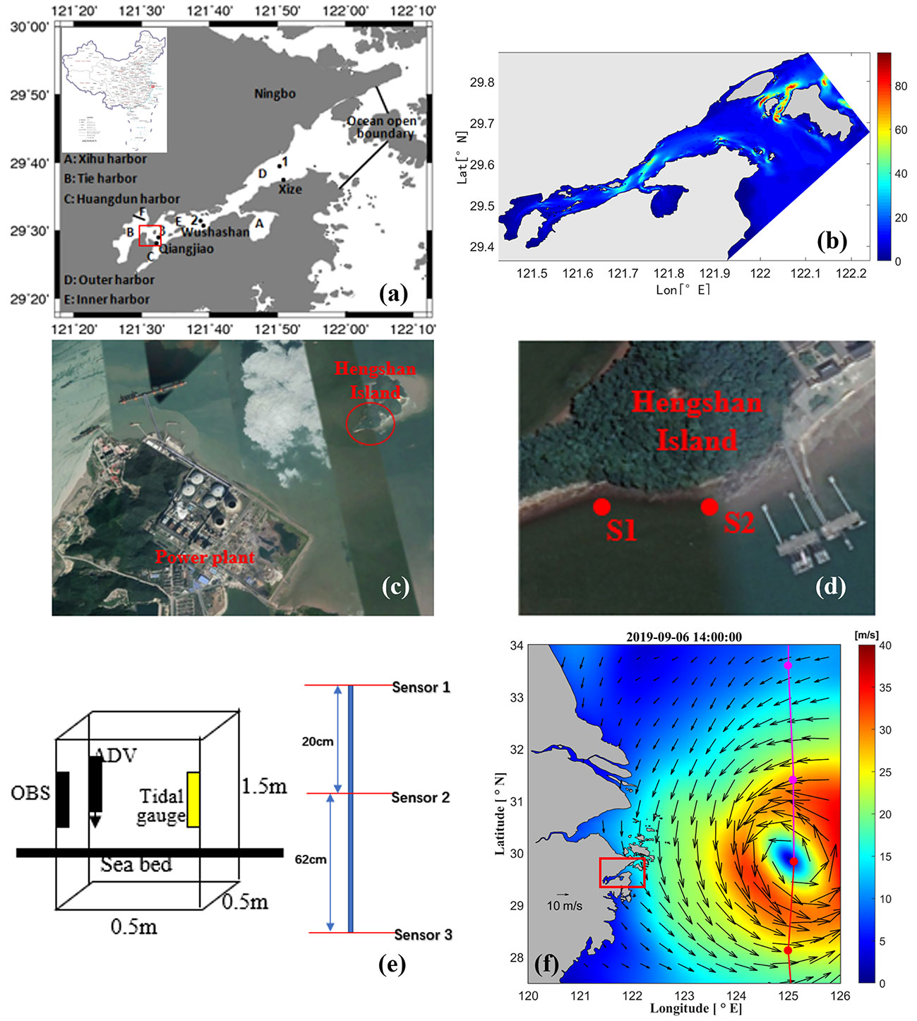
Figure 1 (A) Map of Xiangshan Bay (red box in Xiangshan Bay shows the positions of (C, D). (B) Depth in the bay. (C) Locations of the power plants. (D) Field stations. (E) Arrangement of the instruments and the vertical distribution of temperature sensors below the surface of the tidal flat. (F) The wind field during Typhoon Lingling (13~55 m/s, 930~1002 hPa), and the path of the typhoon during field work (red box shows the location of Xiangshan Bay).
Xiangshan Bay has large tidal flat areas, accounting for more than 30% of the water area (Dong and Su, 1999). The tidal flat is distributed in the range of about 270 km, with a total of 171.3 km2, mainly in the Tie port, Huangdun port, and Xihu port. The width of the tidal flat is approximately 200–1000 m with a slope of 2–8% (You and Jiao, 2011). The intertidal zone is rich in organisms and the average biomass of the intertidal zone reaches 107 g/m2. Previous studies have mainly focused on the coastal reclamation of tidal flats, hydrodynamics, water exchange, and sediment dynamics (Zhao and Yang, 2007; Zeng et al., 2011; Li et al., 2017; Li et al., 2018). The reduction of tidal flats changes the hydrodynamic process and the asymmetric nature of tides (Xia et al., 1997). However, the hydrodynamics in the tidal flat under the interaction of tides-tidal flat-air temperature-thermal discharge requires further investigation.
In this study, we measured the water level, current, water temperature, and turbidity in the tidal flat near the power plants at the head of Xiangshan Bay during Typhoon Lingling. The hydrodynamics near the bottom boundary layer in tidal flats during spring-neap tidal cycles were first studied, and then the thermal dynamics in the tidal flat were investigated. This study provides a field data for future studies on the impact of tidal flats on thermal discharges and thermodynamics in the bay. The field work and data are introduced in Section 2. Section 3 presents the data analysis. The discussion and conclusions are presented in Sections 4 and 5, respectively.
Two field stations, S1 and S2, were selected to conduct field work (Figure 1D). These two field stations were arranged along the coast of Hengshan Island (Figure 1D), which is opposite to the Qiangjiao Power Plant (Figure 1C). Thermal discharge from the Ninghai Power Plant can affect seawater near Hengshan Island. The seabed was sandy with gravel at station S1 and muddy at station S2.
The field work was conducted between August 31 and September 15, 2019, covering an entire spring-neap tidal cycle. This period was in late autumn, which facilitated the capture of the thermal discharge. The field work was conducted in the wet season, and the signal of super Typhoon Lingling (no. 1913) was captured (Figure 1F), which impacted the bay (23−28°C, moderate rain) around September 6, 2019. On August 30, 2019, Lingling (tropical disturbance) occurred near the island of New Guinea, and was upgraded to a tropical depression on September 2, after which the typhoon began to intensify rapidly. The storm was upgraded to a severe tropical storm on September 3. Subsequently, it was upgraded to a super-typhoon. The maximum wind speed exceeded 50 m/s and the central pressure was 900 hPa when Typhoon Lingling passed by the east coast of China (over 2000 km away, in the open East China Sea). From September 5 to 6, 2019, moderate to heavy rains were observed in the central and northern coastal areas of Zhejiang. During the typhoon transit, the rains in the coastal areas of Zhejiang were 30–70 mm, with some over 100 mm.
The instruments were arranged on two frames, and both of them were 0.5 × 0.5 × 1.5 m. Every fame had a tidal gauge, an optical backscatter sensor (OBS), and an acoustic doppler velocimeter (ADV). The probes of the ADV were set 15 cm above the sea bed. The tidal gauge and the OBS were set at the same level above the seabed. A tidal gauge was set to measure the data every minute at a frequency of 4 Hz. The OBS and ADV were set to operate every 10 min. The tidal flat temperature was measured using temperature sensors near S2 station (Figure 1D) in the tidal flat. Temperature sensors were used to measure the temperature of the tidal flat every 10 min. Three sensors were arranged vertically, that is, near the surface of the tidal flat, 20 cm below the surface, and 82 cm below the surface (Figure 1E).
The tidal gauge data were directly extracted and temporally averaged every 10 min to obtain tidal level data. Wave height data were obtained from the tidal gauge fluctuation data. The wave parameters were then calculated.
The OBS data were calibrated with laboratory experiments before the field work. The correlation of the turbidity with the suspended sediment concentration (SSC) was high, indicated by the R2 value of 0.92 and 0.96 at station S1 and S2, respectively (Figure 2). The turbidity data were then converted to suspended sediment concentration values.
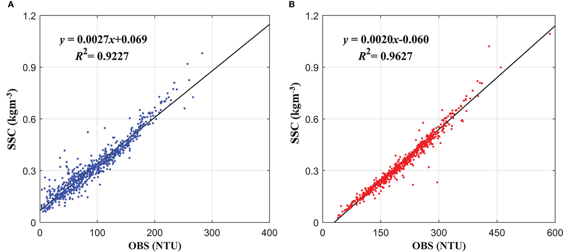
Figure 2 Calibration of the OBS data at station S1 (A) and station S2 (B).
The ADV data were first filtered by the ratio of the signal to noise (SNR) and the correlation of the acoustic signals. Data with SNR values lower than 5% or correlation values lower than 70% were excluded from the series. The phase–space thresholding method (Goring and Nikora, 2002) was then used to remove singular points from the data. A method similar to the Improved Phase-Space Thresholding Method (Wahl, 2003; Parsheh et al., 2010) was also used to calibrate the accuracy of the results.
The turbulence data were obtained using the differences between the instantaneous current velocity and the averaged velocity. Subsequently, the turbulent current and turbulent kinetic energy were calculated.
To determine whether the thermal discharge from the Ninghai Power Plant affected the detectors, we used Landsat 8 data for temperature inversion (http://ids.ceode.ac.cn/query.html, Chen et al., 2018). Landsat 8 includes an Operational Land Imager (OLI) and Thermal Infrared Sensor (TIRS). The OLI land imager includes nine bands with a spatial resolution of 30 m, including a 15-meter panchromatic band with an imaging width of 185 × 185 km. To avoid atmospheric absorption features, OLI readjusts the bands as follows:
where Ts is sea surface temperature, a and b are empirical coefficients.
Landsat-8/TIRS has two thermal infrared channels, and sea surface temperature (SST) remote sensing inversion can use both single- and dual-channel imaging data. The single-window algorithm and the universal single-channel algorithm proposed by Jiménez-Muñoz and Sobrino (2003) were used in this study.
Field stations S1 and S2 were located in the tidal flat of Hengshan Island, which is opposite to the Ninghai Power Plant. Therefore, the sea surface temperature (SST) near the Ninghai Power Plant was retrieved using remote-sensing data (Figure 3). SST data for summer (on July 29, 2019) and winter (on December 2, 2019) were retrieved at the head of the bay. The thermal discharge of the power plant diffused to stations S1 and S2 in the tidal flat of the Hengshan Island. The influence of thermal discharge on the water temperature in winter was more obvious (Figure 3B) than that in summer (Figure 3A). The temperature near the power plant was approximately 8°C higher than that in the vicinity.
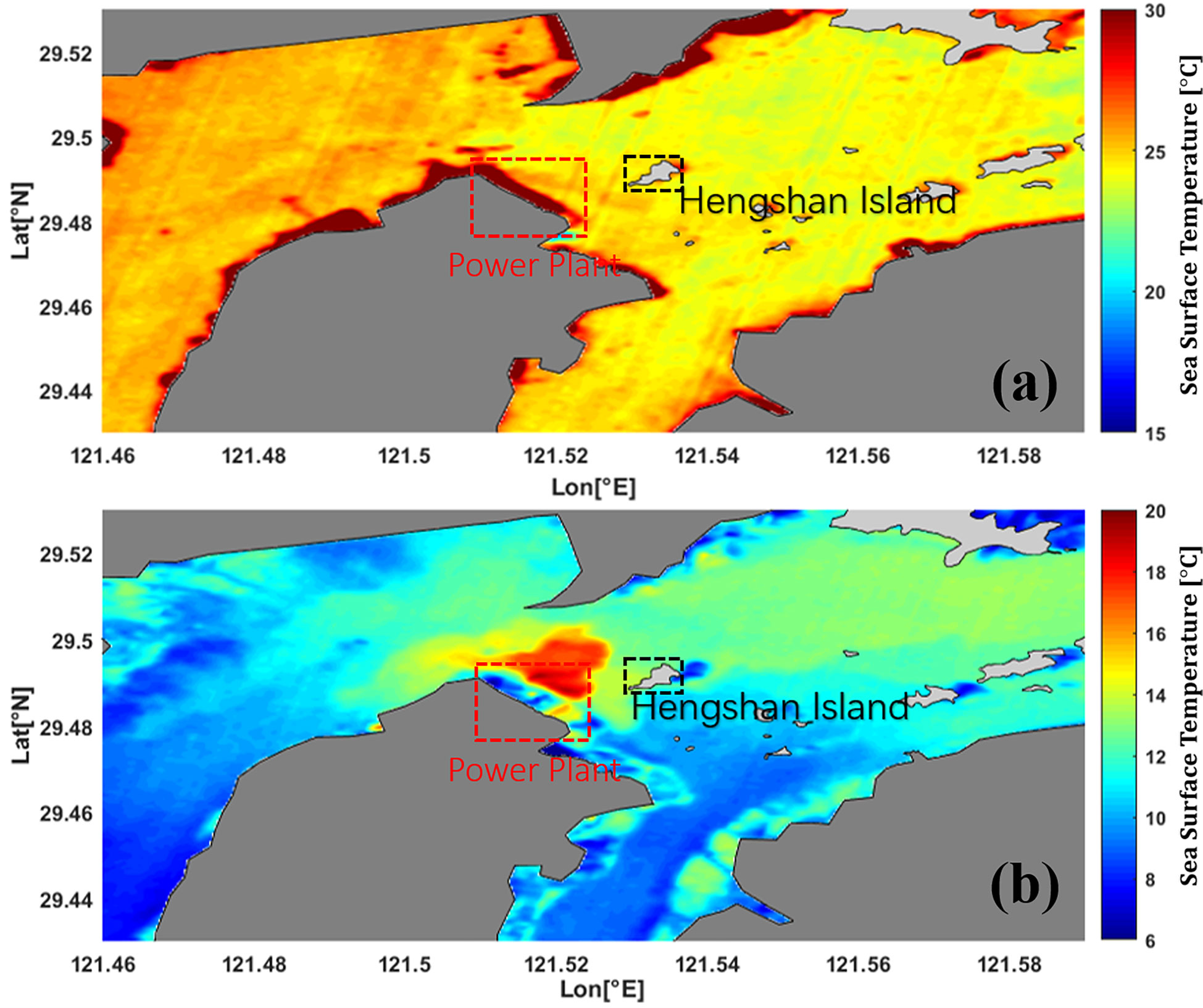
Figure 3 Remote sensing inversion of sea surface temperature (SST) near Ninghai Power Plant: (A) summer (July 29, 2019) and (B) winter (December 2, 2019).
Macro-tidal and semi-diurnal signals during the spring-neap tidal cycle were well captured during the field work (Figure 4A). The tidal ranges at the two stations were nearly 6 m during spring tides and approximately 1 m during neap tides. The storm surge signal was weak and almost undetectable from the water level data because the typhoon was more than 2000 km away from the bay, and the bay was sheltered by its narrow and semi-enclosed morphology. Double peaks during low-slack waters were also captured. According to the results of the harmonic analysis, the interaction of the M2 and M4 tides contributed to the double peaks of sea surface elevation.
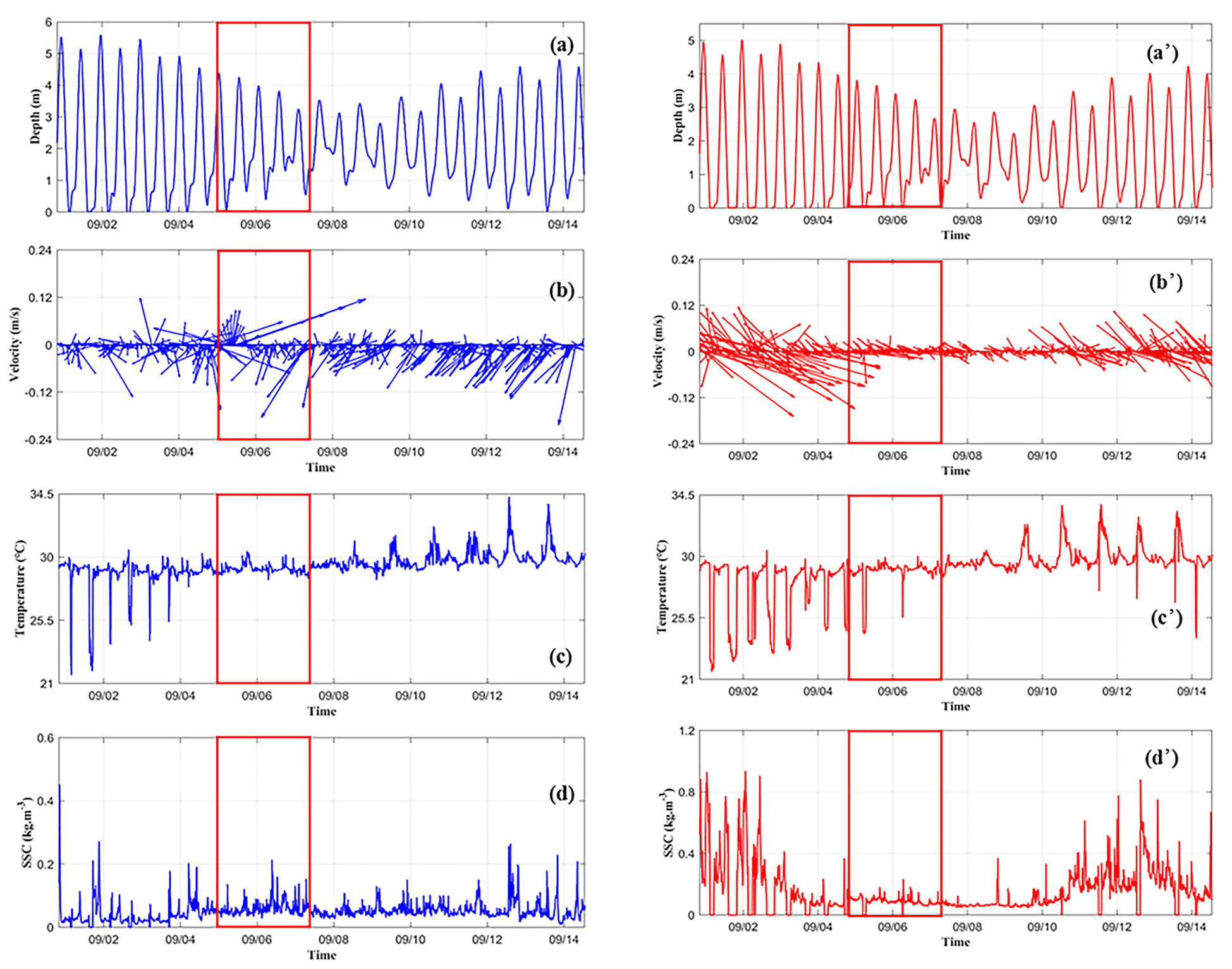
Figure 4 Time series of sea surface levels, currents, temperature, and suspended sediment concentration (SSC) at station S1 (blue lines, (A–D) and S2 (red lines, (A’–D’). The red box indicates the typhoon period.
The currents were weak at the two stations (Figure 4B), with a maximum current speed of approximately 0.5 m/s. The current magnitude and direction at station S1 fluctuated and were disordered. Around September 6, the current speeds at station S1 were high. This is most likely due to the impacts of the Typhoon Lingling. The maximum wind speed near the station during this period exceeded 15m/s, with a northerly wind most of the time. The currents at station S2 were stronger than those at station S1. Current magnitudes at station S2 showed spring-neap and flood-ebb tidal signals, with strong currents during spring tides and weak currents during neap tides. The current directions at station S2 were mainly along the coast in the northwest-southeast direction.
Water temperature at both stations showed an increasing trend during the field work and a periodic pattern in a similar period with the tides (Figure 4C). The sea water temperature fluctuated during the field work, with occasional low temperatures during the first several days and occasional high temperatures during the last several days. This fluctuation was due to the exposure of the temperature sensor to air at this moment, as seen from the zero depth in Figure 4A. The maximum temperature of the seawater at stations S1 and S2 was near 34.5°C, and the minimum temperature was approximately 21°C. The maximum and minimum values of seawater temperature occurred at peak ebb during spring tides when the tidal flats were exposed. Typhoons occurred around the neap tides (red box in Figure 4). When sensors are in seawater, their temperature is affected by the seawater temperature. The water temperature remained near 30°C during most of the field work. However, the temperature fluctuated with large amplitudes from approximately 22°C to 34.5°C during the following spring tides. During the neap tides, the water temperature was stable and remained at approximately 29°C. At station S1 (Figure 4C), the water was occasionally cool (22°C) during high waters and warm during low waters before the typhoon. After the typhoon, the water was warm (>28°C) throughout the observation period. The peak values of water temperature occurred periodically during the slack waters and showed an increasing trend. A similar trend was observed for water temperature at station S2 (Figure 4C). Different patterns of water temperature occurred during the first and second spring tides at both the stations.
The suspended sediment concentration (SSC) at station S2 (muddy seabed) was highly correlated with the tidal dynamics, with large SSC values (~0.9 kg/m3) during spring tides and small values (~0.1 kg/m3) during neap tides (Figure 4D). The SSC values peaked after the high slack waters and were directly affected by the current speed. During spring tides, the SSC values ranged from approximately 0.2 kg/m3 to about 0.9 kg/m3, whereas during neap tides, the SSC values were around ~0.2 kg/m3. SSC values at station S1 (gravel seabed) were much smaller (mostly<0.2 kg/m3) than those at station S2, and showed a fluctuating pattern (Figure 4D). The SSC values were generally smaller than 0.2 kg/m3 through the field work.
Tidal current statistics (Figure 5) during the spring-neap tidal cycle showed that currents at station S1 (Figure 5A) were largely in the southwest direction. At station S2, the currents were in the northwest-southeast direction most of the time (Figure 5C). During the spring tides and neap tides, the current directions had similar distributions to those during the spring neap tidal cycles.
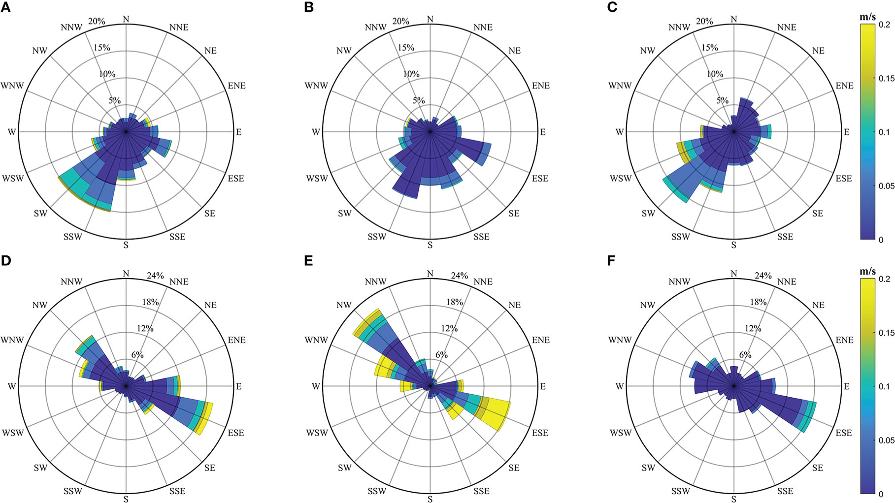
Figure 5 Current statistics during a spring-neap tidal cycle (A, D), a spring tide (B, E), and a neap tide (C, F) at station S1 (A–C) and S2 (D–F).
The residual currents at S1 were 0.01 m/s (181 degree), 0.02 m/s (209 degree), and 0.02 m/s (196 degrees) during the spring tide, neap tide, and spring-neap tidal cycle, respectively. Station S2 had smaller residual currents of less than 0.01 m/s during the spring tide, neap tide, and spring-neap tidal cycle, compared to those at station S1.
The wave parameters calculated using the ADV data are listed in Table 1. The maximum wave height was 0.13 m and 0.14 m and the maximum wave period was about 9.1 s and 11.8 s at station S1 and S2, respectively. The mean wave height was about 0.02 m and mean wave period was about 2.5 s at both of the two stations (Table 1).
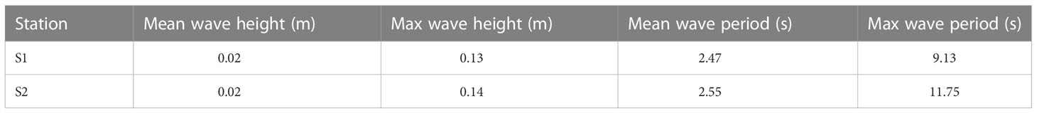
Table 1 Wave data during the observation periods.
The time series of Hs in Figure 6A shows that the significant wave heights at station S1 (blue lines) were slightly smaller than those at station S2 (red lines). The Hs values during the typhoon (around September 5–6, red box) were approximately double (~0.06 m) those at the other time (~0.03 m) at both stations. Large Hs values occasionally occurred at S2.
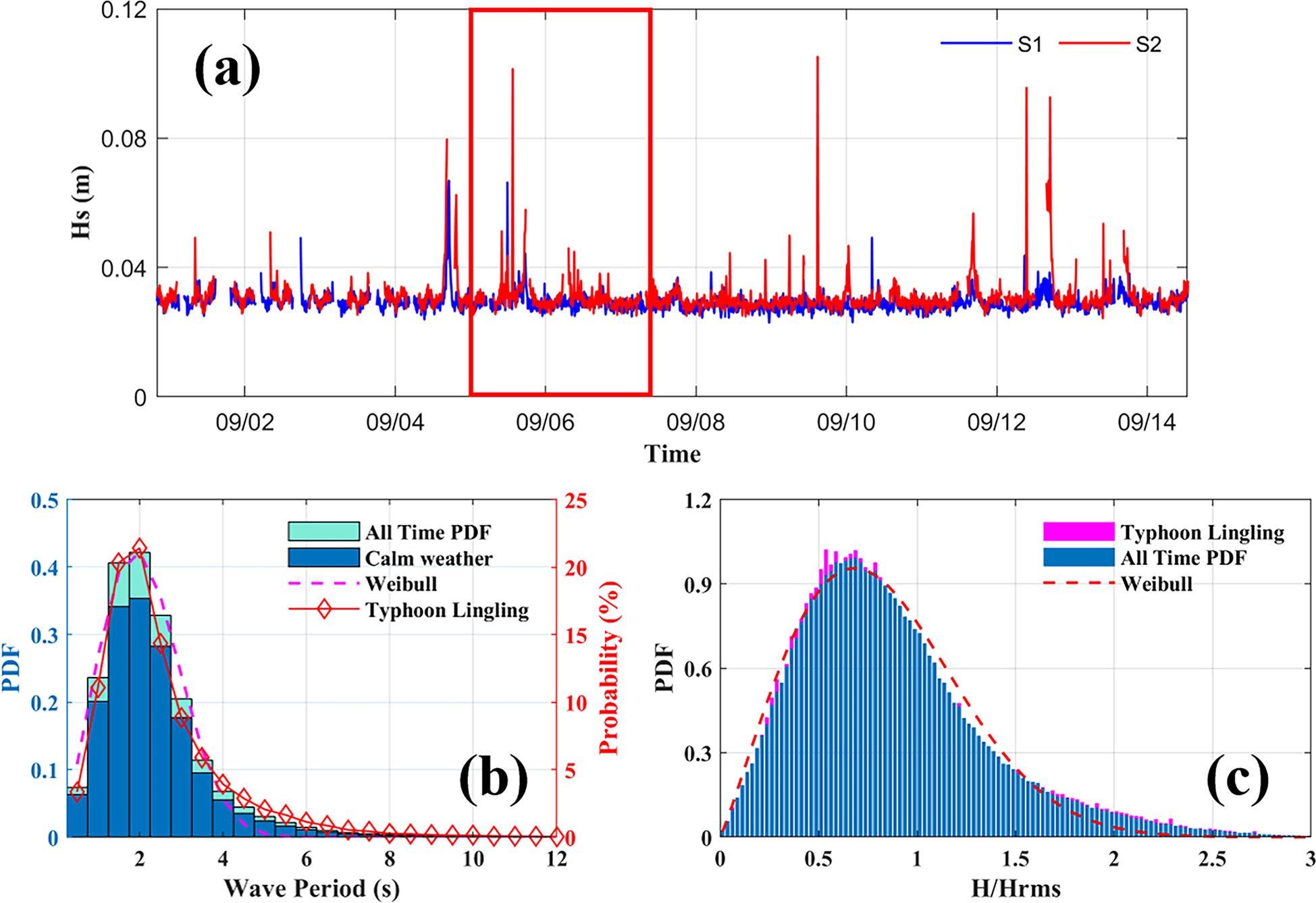
Figure 6 (A) Hs time series at stations S1 (blue lines) and S2 (red lines) calculated using ADV data (red box indicates the typhoon period). (B) Histogram of wave periods and (C) H/Hrms, and the fit of their probability distribution using Weibull distribution function (red lines) at station S1 (RBR data). The probability density of wave periods in calm weather and all time is represented by the blue and cyan histograms in (B), respectively. The wave period distribution during Typhoon Lingling is shown by the red diamond line. Hrms is the root mean square of the wave heights H.
The average wave period was mainly distributed between 1 s and 3 s (Figure 6B). The two sites were located at the head of the bay, where the impacts of winds and swells are small owing to the topography. The significant wave height was small, approximately 0.03 m during calm weather, with a wave period of 1.5~2 s. During the typhoon, the maximum significant wave height was about 0.1 m (Figure 6A).
The distributions of the wave periods and normalized wave heights (H/Hrms) at S1 are shown in Figure 6C. Hrms is the root mean square of wave height H, which indicates the mean wave energy. The histogram of the wave periods (Figure 6B) indicates a skewed wave period distribution, with a peak at 2 s. The normalized wave heights (Figure 6C) show that the wave energy was asymmetrically distributed, with a peak near H/Hrms of 0.6.
The turbulence intensity (I) and turbulent kinetic energy (TKE) were calculated as follows:
where is the averaged current velocity, u’rms is the room mean square of the turbulent current velocity, and u’, v’, and w’ are the turbulent current velocities in the x, y, and z directions, respectively.
As shown in Figure 7, the turbulent intensity at stations S1 and S2 was high, as indicated by the high values of I. The turbulent TKE at station S1 (Figure 7A) was higher than that at station S2 (Figure 7B), and the TKE values at station S1 were largely double those at station S2. The TKE magnitudes showed obvious spring-neap signals and flood-ebb variations at station S2, with higher TKE during spring tides and lower TKE during neap tides. There were small spring-neap variations in TKE at station S1.
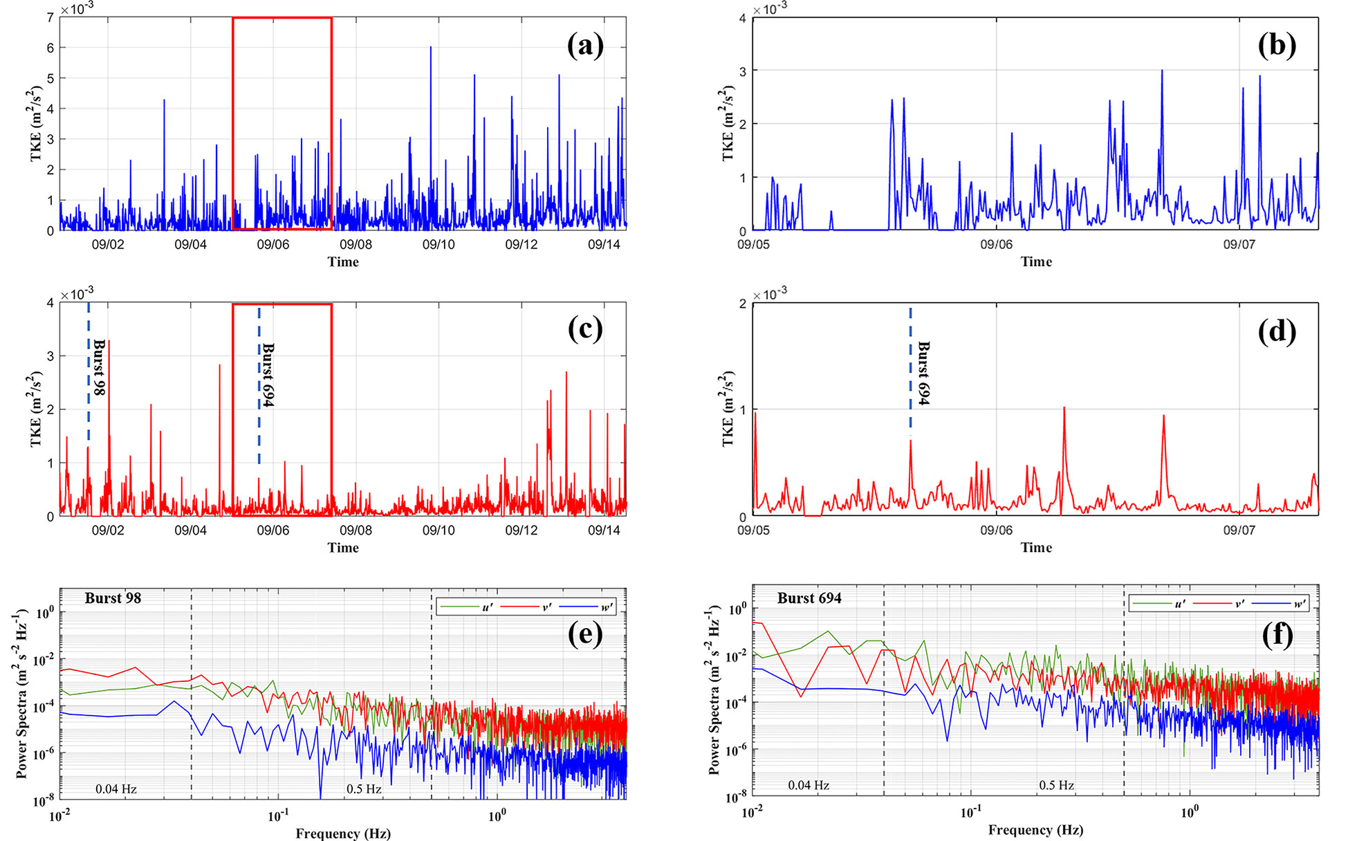
Figure 7 Time series of TKE at station S1 (A, B) and S2 (C, D) during Typhoon Lingling, respectively (red boxes indicate the typhoon periods). Power spectra plots of the three current components during normal conditions (E) and Typhoon Lingling (F). The frequency is indicated by the gray dashed lines, which are 0.04 Hz and 0.5 Hz, respectively.
Utilizing the power spectrum analysis, the properties of the velocity fluctuation (u'/v'/w') in the frequency domain wer eexamined (Li et al., 2022; Chang et al., 2019). As shown in Figures 7E, F, the typhoon increased both the horizontal and vertical energy. In burst 98 (Hs = 0.05 m, T = 2.75 s, h = 2.81 m), the horizontal energy in the wave frequency range (0.04-0.5 Hz) was greater (Figure 7E, green and red lines), demonstrating that the horizontal wave orbital velocities predominated the seawater turbulence. During the typhoon (e.g., burst 694, Hs = 0.10 m, T = 5.42 s, h = 2.30 m), the energy of the horizontal and vertical velocity fluctuations and their corresponding peak periods increased (Figure 7C, D).
Waves in shallow-water areas flowed elliptically. The horizontal and vertical velocity components of the waves are given by:
where H, σ, k, and h represent the wave height, angular frequency, wavenumber, and water depth, respectively. Coshkh and sinhkh were simplified to 1 and kh, respectively, for shallow-water waves. The wave ellipses grow flatter toward the bottom, indicating that the vertical orbital velocities degenerated faster than the horizontal ones (Dean and Dalrymple, 1991; Bian et al., 2020; Li et al., 2022). As a result, the horizontal energy (red and green lines in Figures 7E, F) was greater than the vertical energy in the wave frequency range (blue lines in Figures 7E, F).
The temperature variation in the tidal flat was largest near the seabed surface (Figure 8, red lines), followed by the second layer (20 cm below the tidal flat surface, aqua blue). The third layer had the smallest variation in temperature (82 cm below the tidal flat surface, sky blue). This is related to the more frequent heat exchange between the tidal flat surface, water, and the atmosphere. Peaks (low or high) in temperature occasionally occurred. The lowest temperature was approximately 15°C, and the highest temperature was approximately 35°C. The highest and lowest temperatures occurred near the surface of the tidal flat (red lines in Figure 8). The temperature peaks might have been caused by the air temperature because the sensor was located near the seabed surface. Simultaneously, the sensor temperature was also affected by the tidal flat. The specific heat capacity of the tidal flat was less than that of the water body; therefore, the tidal flat temperature increased faster than the sea water temperature.
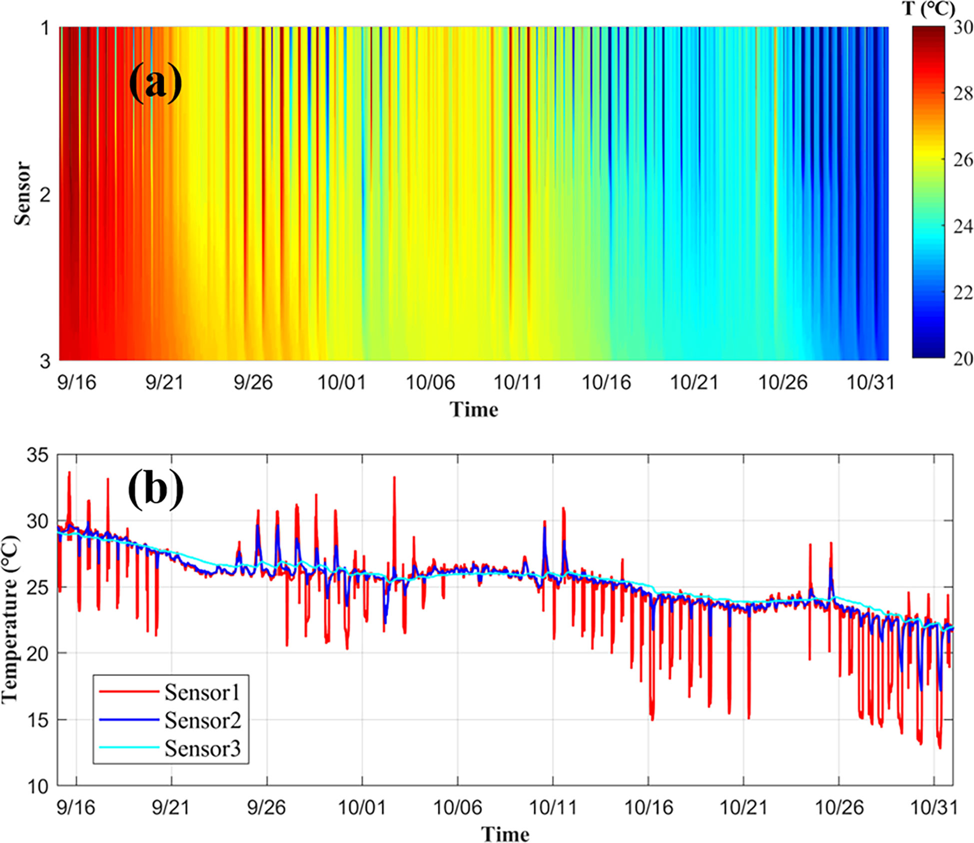
Figure 8 Time series of temperature near station S2 in the tidal flat: (A) color contours and (B) time series. Sensor 1, 2, and 3 in the legend indicate the sensor at the seabed surface and 20 cm and 82 cm inside the mud, respectively (from September 15 to October 31, 2019).
As seen from the time series of the temperature data and tide level data (Figure 9), the temperature fluctuation was small (mostly within 1°C) during the neap tides and large (>4°C) during the spring tides. The water temperature fluctuated around 29−30°C during the field period. Temperature peaks/troughs occurred during low slack waters during the spring tides, with negative troughs occurring during the first spring tidal period (September 1−6) and positive peaks occurring during the second spring tidal period (September 9−14). In the first spring tidal period, temperature troughs occurred in the low slack waters during the same periods of exposure of the tidal flat. In the second spring tidal period, temperature peaks occurred in low-slack waters. During the neap tides, temperature peaks and troughs occurred during low slack water periods and high slack water periods, respectively.
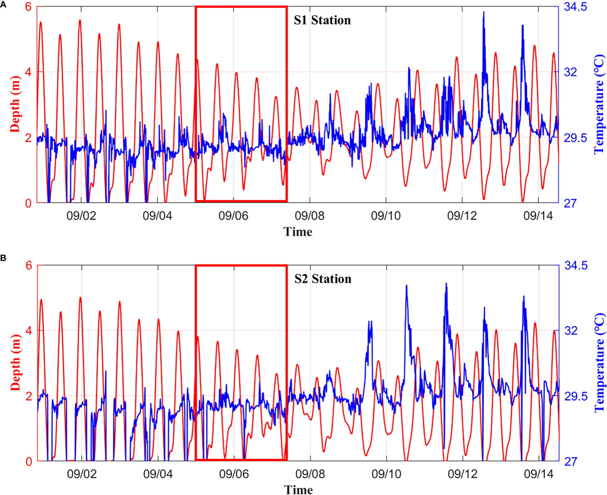
Figure 9 Relationship between sea water temperature and water level at (A) station S1 and (B) station S2 (red box indicates typhoon periods).
Water temperature was affected by the combined effects of the ocean and air. During neap tides, the water depth changes were small, and the water temperature was less affected by the atmosphere. During the spring tides, the water depth was shallow in the spring low-slack waters, and the water temperature was sensitive to the atmosphere and tidal flat. This indicates that the temperature fluctuated with the ocean and air temperatures. In the low slack waters of the first spring tidal period, the sensor was exposed to air and showed air temperature instead of water temperature. When the water depth is shallow, the seawater temperature is sensitive to the atmosphere. As Typhoon Lingling impacted the bay around September 6, 2019 (during the first spring tidal periods), the air temperature was low (22°C on September 2), compared with that during the second spring tidal cycle (32°C on September 3).
Figure 10 shows the time variation of water flux per unit width at the two stations. At station S1 (Figure 10A), the water fluxes were mainly along the shore in the west-east and south-north directions, with large eastward and southward fluxes, as indicated by the large values in the x direction and large negative values in the y direction. In addition, during the typhoon, the water fluxes at station S1 shifted from west to east. At station S2 (Figure 10B), the water fluxes were large in the east and north directions during the field work. The net water fluxes at station S1 were mainly seawards. The net water flux at station S2 was mainly landward.
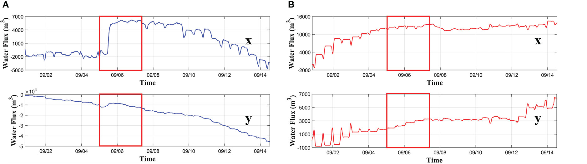
Figure 10 Time series of water fluxes at station S1 (A) and S2 (B) (red box indicates typhoon periods).
Comparing the heat fluxes in the unit widths of the two stations (Figure 11), the changes in the heat fluxes at the two stations were similar. Large or small variations occurred during the spring/neap tides. These changes may be due to the shallow tidal level and large temperature changes at that time. During the typhoon, the change in seawater temperature decreased, and the change in heat flux was small.
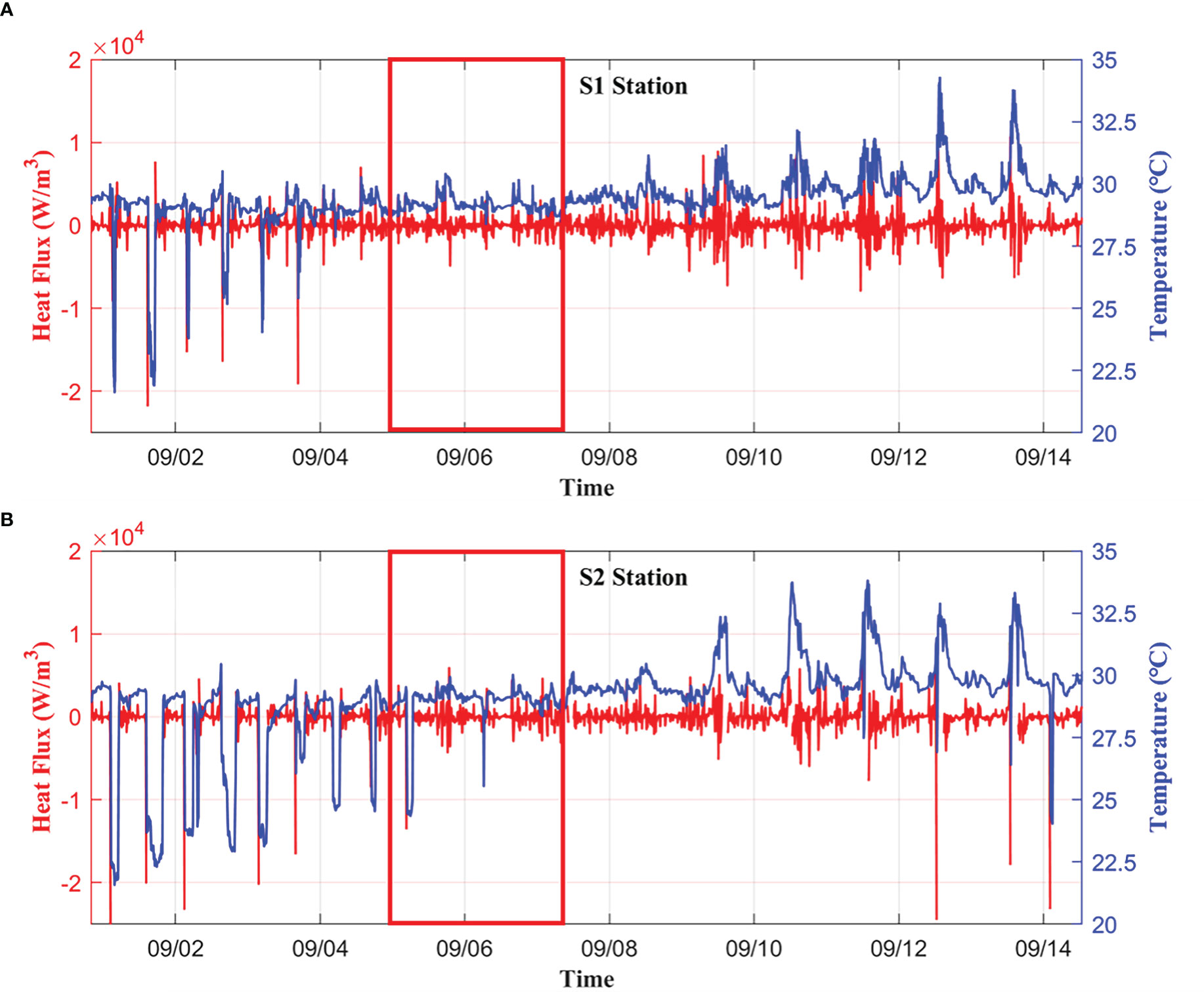
Figure 11 Relationship between heat fluxes and sea water temperature at (A) station S1 and (B) station S2.
The sea water temperature fluctuated at stations S1 and S2. To study the variation and mechanism of sea temperature during the observation period, we performed the empirical mode decomposition (EMD) analysis on the temperature data (Figure 12). EMD is a signal processing method (Huang et al., 1998; Huang et al., 1999) that decomposes a signal according to the time scale characteristics of the data itself. It has advantages in dealing with nonstationary and nonlinear data, and decomposes a complex signal into a limited number of eigenmode functions (IMFs).
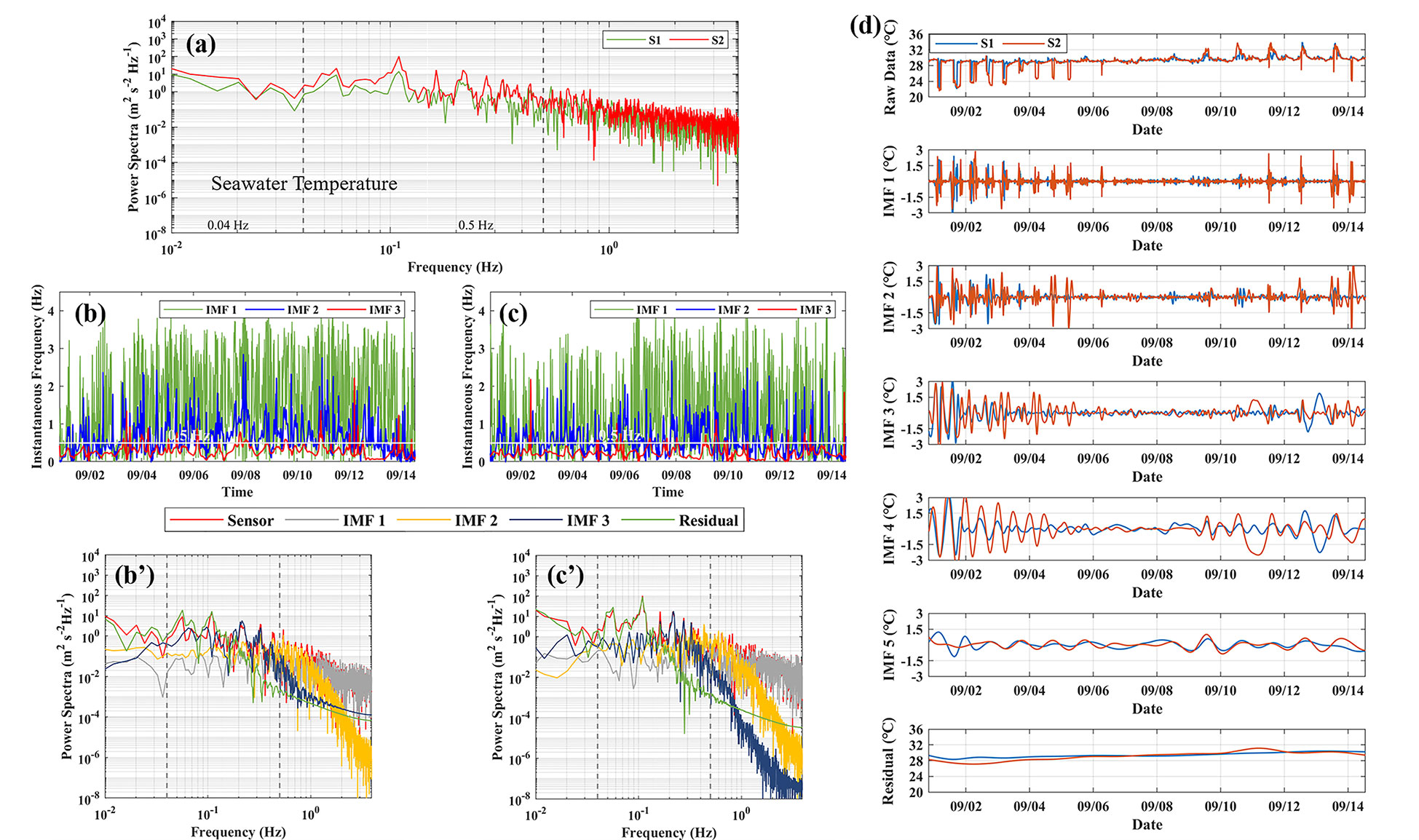
Figure 12 (A) The power spectra of the sea water temperature: S1 (green) and S2 (red). The gray dashed lines indicate the frequency of 0.04 Hz and 0.5 Hz, respectively. (B, C) Instantaneous frequency time series of IMF 1–3 of the sea water temperature: (B) S1 and (C) S2. (B’-C’) The power spectra of the sea water temperature (red) and its decomposed IMFs and residual: (B’) S1 and (C’) S2. (D) Time series of EMD decomposition results of sea water temperature. From top to bottom: raw data, IMF 1-5, and residual (August 31 to September 15, 2019).
The power spectra of the seawater temperature are shown in Figure 12A. Seawater temperature was decomposed using the EMD method. The instantaneous frequency time series (Figure 12B, C) and power spectrum analysis of the IMFs (Figures 12B', C') were obtained by calculation. Small-scale features (>0.5 Hz) (e.g., turbulence) can be detected at instantaneous frequencies of IMF 1 and IMF 2. IMF 3 represents relatively low-frequency motion. The peak frequencies of IMF 1 at both stations S1 and S2 were mostly in the turbulent frequency range (>0.5 Hz). IMF 2 had substantial turbulence information at its peak frequencies, which were in the wave frequency range (0.04–0.5 Hz). IMF 1 and IMF 2 were therefore classified as the turbulent components.
Each IMF component represents the change in different scales, and each IMF component is a narrow-band signal (Figure 12D). IMF 1 had the largest amplitude and highest frequency. The frequency decreased in IMF 2 and 3, and the amplitude also decreased. The temperature fluctuation alternated between large and small fluctuations, which was the same trend as that observed for the spring-neap tidal cycle. When decomposed into five IMF components, the overall trend of temperature increased, as shown by the residual (Figure 12D). This indicates that the seawater temperature at both stations increased slightly during the field work (Figure 12D).
The tidal flat temperature of each sensor was decomposed into a series of IMFs using Hilbert transform (Huang et al., 1998). The instantaneous frequency time series and power spectrum analysis of the IMFs decomposed using EMD are shown in Figure 13. Sensor 1 in the surface layer exhibited the largest variation in amplitude and showed a high degree of agreement with the original data (Figure 13A). Sensor 3 exhibited the smallest amplitude variations. Sensors 2 and 3 had similar trends and energies in the turbulent frequency band (>0.5 Hz), as both sensors were in the subsurface layer of the tidal flat.
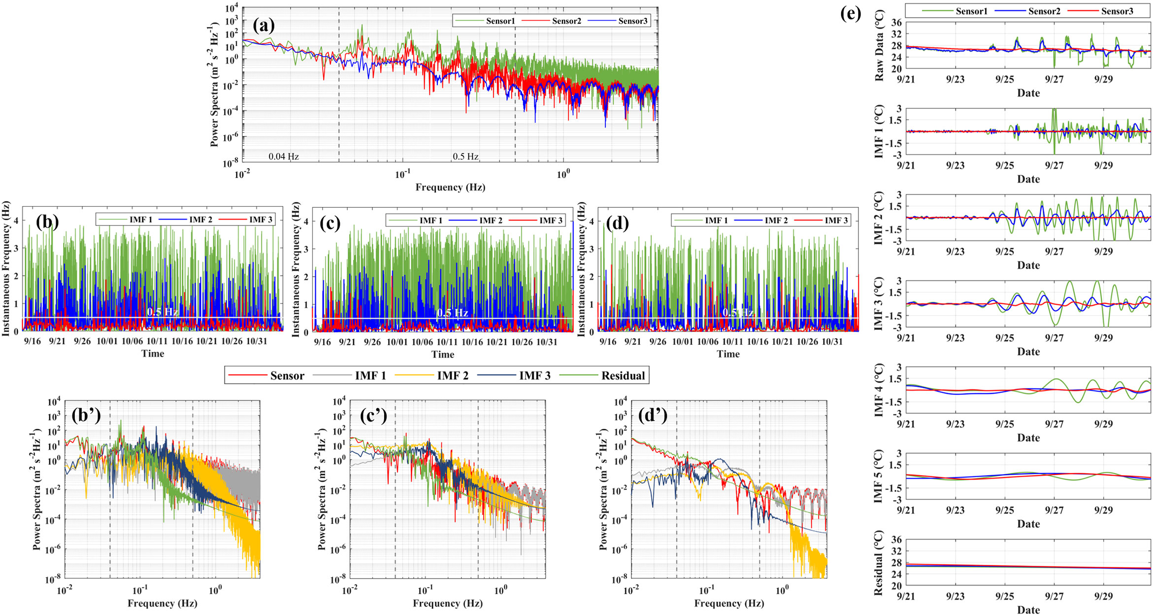
Figure 13 (A) The power spectra of the tidal flat temperature: sensor 1 (green), sensor 2 (red), and sensor 3 (blue). (B–D) Instantaneous frequency time series of IMF 1–3 of the tidal flat temperature: (B) sensor 1, (C) sensor 2, and (D) sensor 3. (B’–D’) The power spectra of the tidal flat temperature (red) and its decomposed IMFs and residual: (B’) sensor 1, (C’) sensor 2, and (D’) sensor 3. (E) Time series of EMD decomposition results of tidal flat temperature. From top to bottom: raw data, IMF 1−5, and residual (from September 21 to October 1, 2019).
Each IMF component had a relatively stable quasi-period, and the variance contribution was used to express the effects of the amplitude and frequency on the raw signal data. The IMFs of the seawater temperature and surface tidal flat temperature were similar, but the IMFs of the middle (20 cm below the seabed) and bottom (82 cm below the seabed) layers in the tidal flat were less correlated. This is because both the sea water temperature and surface tidal flat temperature are subject to similar sea-air-tidal flat interactions.
The variance contribution of the IMF 3 component was large, and the average period of the IMF 3 component was close to 24 h, which was mainly due to the daily variation in weather and influenced by the heat flux cycle (Figure 13E). The average period of IMF 2 was close to 12.42 h, which was mainly due to the tidal effect caused by the irregular semi-diurnal tide characteristics in the bay. Therefore, the temperature fluctuations of seawater and tidal flats were mainly affected by air temperature and tides. Thermal discharges spread with tide, with higher temperatures during ebb tides and lower temperatures during flood tides (Figure 9), as the power plant was located upstream of the field stations (Figure 3B). Therefore, the second most influential factor of the temperature change (12.42 h) may be caused by thermal discharges. The average period of IMF 1 was less than 4 h, which may be related to the inundation of the tidal flats or exposure. The peak frequencies of IMF 1 for tidal flat temperature decomposition were mostly in the turbulent frequency range (>0.5 Hz), which may thus be subject to waves. The overall trend of the tidal flat temperature decreased during field work, as shown by the residuals (Figure 13E).
In this study, we take the macro-tidal narrowed Xiangshan Bay as an example to study the hydrodynamics and thermal characteristics of tidal flats, considering the impacts of typhoons and thermal discharges. Field work was conducted to measure the water level, current, water temperature, tidal flat temperature, and turbidity data at the bottom level of the tidal flat near the power plant. The field data covered a full spring-neap tidal cycle and were well calibrated to investigate the hydrodynamics in the tidal flat.
Data analysis showed that the spring-neap tidal cycles at the sea surface level were well captured at both stations. The tidal flat was occasionally exposed to air (30 min). The maximum tidal ranges were 5.5 m and 1.5 m during spring and neap tides, respectively, at the two stations. The current velocity (<0.2 m/s) and waves (<0.15 m) at the field stations were weak, and the direction of flow was controlled by the geomorphology, even during Typhoon Lingling. Water was more turbid at station S2 (<0.9 kg/m3) than at station S1 (<0.2 kg/m3). The maximum value of seawater temperature at station S1 was greater than that at station S2. The impact of thermal discharge on water temperature was weak during field work.
The sea water temperature and tidal flat temperature were found to be affected by the tidal cycles. Both sea water temperature and surface tidal flat temperature were subject to sea−air−tidal flat interactions. Temperature fluctuations in seawater and tidal flats were mainly affected by air temperature and tides. According to the residuals obtained using the EMD method, seawater temperatures at both stations increased during the field work period. The temperature in the surface layer of the tidal flat had the largest variation, whereas the temperature inside the tidal flat (sensor S3, 82 cm below) had the smallest variation. The tidal flat temperature at sensors S2 (20 cm below) and S3 had similar trends and energies in the small-scale frequency band (>0.5 Hz). The IMFs of seawater temperature and surface tidal flat temperature were similar, while the IMFs of the middle and bottom layers were less closely correlated.
The original contributions presented in the study are included in the article/supplementary material. Further inquiries can be directed to the corresponding authors.
LL, JX, and PL: manuscript writing, data analysis, methodology, modelling, organization. HW, GK and YR: discussion and field work. All authors contributed to the article and approved the submitted version.
This research was supported by the National Natural Science Foundation of China (41976157, 42076177), the Science Technology Department of Zhejiang Province (2020C03012, 2022C03044, U1709204), and the State Key Laboratory of Satellite Ocean Environment Dynamics, MNR, China (QNHX1807).
The authors declare that the research was conducted in the absence of any commercial or financial relationships that could be construed as a potential conflict of interest.
All claims expressed in this article are solely those of the authors and do not necessarily represent those of their affiliated organizations, or those of the publisher, the editors and the reviewers. Any product that may be evaluated in this article, or claim that may be made by its manufacturer, is not guaranteed or endorsed by the publisher.
Bian C. W., Liu X. L., Zhou Z., Chen Z. X., Wang T., Gu Y. Z. (2020). Calculation of winds induced bottom wave orbital velocity using the empirical mode decomposition method. J. Atmos. Ocean Technol. 37 (5), 889–900. doi: 10.1175/JTECH-D-19-0185.1
Chang Y., Chen Y. N., Li Y. (2019). Flow modification associated with mangrove trees in a macro-tidal flat, southern China. Acta Oceanol Sin. 38 (2), 1–10. doi: 10.1007/s13131-018-1163-y
Chang Y., Chen Y. N., Wang Y. P. (2020). Field measurements of tidal flows affected by mangrove seedlings in a restored mangrove swamp, southern China. Estuarine Coast. Shelf Sci. 235, 106561. doi: 10.1016/j.ecss.2019.106561
Chen Y. N., Li Y., Thompson C., Wang X. K., Cai T. L., Chang Y. (2018). Differential sediment trapping abilities of mangrove and saltmarsh vegetation in a subtropical estuary. Geomorphology 318, 270–282. doi: 10.1016/j.geomorph.2018.06.018
Chen L. Z., Zeng X. Q., Tam N. F. Y., Lu W. Z., Luo Z. K., Du X. N., et al. (2012). Comparing carbon sequestration and stand structure of monoculture and mixed mangrove plantations of sonneratia caseolaris and s. apetala in southern China. For. Ecol. Manage. 284, 222–229. doi: 10.1016/j.foreco.2012.06.058
Chen H. Y., Zhu L., Li J. G., Fan X. Y. (2018). A comparison of two mono-window algorithms for retrieving sea surface temperature from Landsat8 data in coastal water of hongyan river nuclear power station. Remote Sens. Land Resour. 30 (01), 45–53. doi: 10.6046/gtzyyg.2018.01.07
Cho Y. K., Kim M. O., Kim B. C. (2000). Sea Fog around the Korean peninsula. J. Appl. Meteorol 39 (12), 2473–2479. doi: 10.1175/1520-0450(2000)039<2473:SFATKP>2.0.CO;2
Cho Y. K., Kim T. W., You K. W., Park L. H., Moon H. T., Lee S. H., et al. (2005). Temporal and spatial variabilities in the sediment temperature on the baeksu tidal flat, Korea. Estuarine Coast. Shelf Sci. 65 (1-2), 302–308. doi: 10.1016/j.ecss.2005.06.010
Dean R. G., Dalrymple R. N. (1991). Water Wave Mechanics for Engineersand Scientists, World Scientific Publishing Company
Dong L. X., Su J. L. (1999). Tide response and tide wave distortion study in the xiangshan bay. Acta Oceanol Sin. 21 (03), 1–6.
Dong Y., Zuo L., Ma W., Chen Z., Cui L., Lu S. (2021). Phytoplankton community organization and succession by sea warming: A case study in thermal discharge area of the northern coastal seawater of China. Mar. pollut. Bull. 169, 112538. doi: 10.1016/j.marpolbul.2021.112538
Friedlander M., Levy D., Hornung H. (1996). The effect of cooling seawater effluents of a power plant on growth rate of cultured gracilaria conferta (Rhodophyta). Hydrobiologia 332 (3), 167–174. doi: 10.1007/BF00031922
Gao J. H., Shi Y., Sheng H., Kettner A. J., Yang Y., Jia J. J., et al. (2019). Rapid response of the changjiang (Yangtze) river and East China Sea source-to-sink conveying system to human induced catchment perturbations. Mar. Geol 414, 1–17. doi: 10.1016/j.margeo.2019.05.003
Goring D. G., Nikora V. I. (2002). Despiking acoustic Doppler velocimeter data. J. hydraulic Eng. 128 (1), 117–126. doi: 10.1061/(ASCE)0733-9429(2002)128:1(117)
Gu X. X., Zhao H. W., Peng C. J., Guo X. D., Lin Q. L., Yang Q., et al. (2022). The mangrove blue carbon sink potential: Evidence from three net primary production assessment methods. For. Ecol. Manage. 504, 119848. doi: 10.1016/j.foreco.2021.119848
Huang N. E., Shen Z., Long S. R. (1999). A new view of nonlinear water waves: the Hilbert spectrum. Annu. Rev. fluid mechanics 31, 417–457. doi: 10.1146/annurev.fluid.31.1.417
Huang N. E., Shen Z., Long S. R., Wu M. C., Shih H. H., Zheng Q., et al. (1998). The empirical mode decomposition and the Hilbert spectrum for nonlinear and non-stationary time series analysis. Proc. R. Soc. London. Ser. A: mathematical Phys. Eng. Sci. 454 (1971), 903–995. doi: 10.1098/rspa.1998.0193
Huang X. Q., Ye H. F. (2014). Monitoring and impact assessment of temperature rise of thermal discharge of xiangshan bay (Beijing: China Ocean press), 301pp.
Jiang C. P., Xu Z. L., Chen J. J., Sun L. F., Que J. L. (2016). Effects of the thermal discharge from qinshan nuclear plant on the distribution pattern of fish. J. Fishery Sci. China 23 (2), 478–488. doi: 10.3724/SP.J.1118.2016.15285
Jiménez-Muñoz J. C., Sobrino J. A. (2003). A generalized single-channel method for retrieving land surface temperature from remote sensing data. J. Geophys. Res. Atmos. 108 (D22). doi: 10.1029/2003JD003480
Kim T. W., Cho Y. K. (2009). Heat flux across the surface of a macrotidal flat in southwest Korea. J. Geophys. Res. Oceans 114 (C7), C07027:1–C07027:11. doi: 10.1029/2008JC004966
Kim T. W., Cho Y. K. (2011). Calculation of heat flux in a macrotidal flat using FVCOM. J. Geophys. Res. Oceans 116 (C3), C03010:1–C03010:16. doi: 10.1029/2010JC006568
Kim T. W., Cho Y. K., Dever E. P. (2007). An evaluation of the thermal properties and albedo of a macrotidal flat. J. Geophys. Res. Oceans 112 (C12), C12009-1-C12009-9-0.
Kong G., Li L., Guan W. (2022). Influences of tidal flat and thermal discharge on heat dynamics in xiangshan bay. Front. Mar. Sci. 293. doi: 10.3389/fmars.2022.850672
Li J. S., Chen X. D., Townend I., Shi B. W., Du J. B., Gao J. H., et al. (2021). A comparison study on the sediment flocculation process between a bare tidal flat and a clam aquaculture mudflat: The important role of sediment concentration and biological processes. Mar. Geol 434, 106443. doi: 10.1016/j.margeo.2021.106443
Li L., Fang T. Y., Guan W. B., Zhao X. Z. (2015). The influence of the decrease of tidal flat on the tide of xiangshan bay. 17th China Offshore Eng. Symposium 144–148.
Li L., Guan W., He Z., Yao Y., Xia Y. (2017). Responses of water environment to tidal flat reduction in xiangshan bay: Part II locally re-suspended sediment dynamics. Estuarine Coast. Shelf Sci. 198, 114–127. doi: 10.1016/j.ecss.2017.08.042
Li L., Guan W., Hu J., Cheng P., Wang X. H. (2018). Responses of water environment to tidal flat reduction in xiangshan bay: Part I hydrodynamics. Estuarine Coast. Shelf Sci. 206, 14–26. doi: 10.1016/j.ecss.2017.11.003
Li J. S., Wang Y. P., Du J. B., Luo F., Xin P., Gao J. H., et al. (2020). Effects of meretrix meretrix on sediment thresholds of erosion and deposition on an intertidal flat. Ecohydrol Hydrobiol 21 (1), 129–141. doi: 10.1016/j.ecohyd.2020.07.002
Li L., Ren Y. H., Wang X. H., Xia Y. Z.. (2022). Sediment dynamics on a tidal flat in macro-tidal Hangzhou Bay during Typhoon Mitag. Cont. Shelf Res. 237, 104684. doi: 10.1016/j.csr.2022.104684
Lin Z., Zhan H. (2000). Effects of thermal effluent on fish eggs and larvae in waters near daya bay nuclear plant. Tropic oceanol/Redai Haiyang. Guangzhou 19 (1), 44–51. doi: 10.3969/j.issn.1009-5470.2000.01.007
Lin J., Zou X., Huang F., Yao Y. (2021). Quantitative estimation of sea surface temperature increases resulting from the thermal discharge of coastal power plants in China. Mar. Pollut. Bull. 164, 112020. doi: 10.1016/j.marpolbul.2021.112020
Liu B., Cai T. L., Chen Y. N., Yuan B. Y., Wang R., Xiao M. (2022). Sediment dynamic changes induced by the presence of a dyke in a scirpus mariqueter saltmarsh. Coast. Eng. 174, 104119. doi: 10.1016/j.coastaleng.2022.104119
Lu W. Z., Chen L. Z., Wang W. Q., Tam N. F. Y., Lin G. H. (2013). Effects of sea level rise on mangrove avicennia population growth, colonization and establishment: Evidence from a field survey and greenhouse manipulation experiment. Acta Oecologica 49, 83–91. doi: 10.1016/j.actao.2013.03.009
Lunstrum A., Chen L. Z. (2014). Soil carbon stocks and accumulation in young mangrove forests. Soil Biol. Biochem. 75, 223–232. doi: 10.1016/j.soilbio.2014.04.008
Parsheh M., Sotiropoulos F., Porté-Agel F. (2010). Estimation of power spectra of acoustic-doppler velocimetry data contaminated with intermittent spikes. J. Hydraulic Eng. 136 (6), 368–378. doi: 10.1061/(ASCE)HY.1943-7900.0000202
Peng H. (2013). Numerical study of water exchange in xiangshan port (Hangzhou: Zhejiang University).
Piccolo M. C., Perillo G. M. E., Daborn G. R. (1993). Soil temperature variations on a tidal flat in minas basin, bay of fundy, Canada. Estuarine Coast. Shelf Sci. 36 (4), 345–357. doi: 10.1006/ecss.1993.1021
Rajadurai M., Poornima E. H., Narasimhan S. V., Rao V. N. R., Venugopalan V. P. (2005). Phytoplankton growth under temperature stress: Laboratory studies using two diatoms from a tropical coastal power station site. J. Thermal Biol. 30 (4), 299–305. doi: 10.1016/j.jtherbio.2005.01.003
Rinehimer J. P., Thomson J. T. (2014). Observations and modeling of heat fluxes on tidal flats. J. Geophysical Research: Oceans 119 (1), 133–146. doi: 10.1002/2013JC009225
Roemmich D., McGowan J. (1995). Climatic warming and the decline of zooplankton in the California current. Science 267 (5202), 1324–1326. doi: 10.1126/science.267.5202.1324
Roy P., Rao I. N., Martha T. R., Kumar K. V. (2022). Discharge water temperature assessment of thermal power plant using remote sensing techniques. Energy Geosci. 3 (2), 172–181. doi: 10.1016/j.engeos.2021.06.006
Salgueiro D. V., De Pablo H., Nevesa R., Mateus M. (2015). Modelling the thermal effluent of a near coast power plant (Sines, Portugal). Rev. Gestão Costeira Integrada-Journal Integrated Coast. Zone Manage. 15 (4), 533–544. doi: 10.5894/rgci577
Shen P. Y. (2003). A study on farmign capacity and sustained development of aquaculture in xiangshan port. Modern Fisheries Inf. 17 (7), 22–24. doi: 10.3969/j.issn.1004-8340.2002.07.007
Shi B. W., Cooper J. R., Li J. S., Yang Y., Yang S. L., Luo F., et al. (2019). Hydrodynamics, erosion and accretion of intertidal mudflats in extremely shallow waters. J. Hydrol 573, 31–39. doi: 10.1016/j.jhydrol.2019.03.065
Shi B. W., Wang Y. P., Wang L. H., Li P., Gao J. H., Xing F., et al. (2018). Great differences in the critical erosion threshold between surface and subsurface sediments: A field investigation of an intertidal mudflat, jiangsu, China. Estuarine Coast. Shelf Sci. 206, 76–86. doi: 10.1016/j.ecss.2016.11.008
Shi B. W., Yang S. L., Temmerman S., Bouma T., Ysebaert T., Wang S. K., et al. (2021). Effect of typhoon-induced intertidal-flat erosion on dominant macrobenthic species (Meretrix meretrix). Limnol Oceanogr 66 (12), 4197–4209. doi: 10.1002/lno.11953
Wahl T. L. (2003). Discussion of “Despiking acoustic doppler velocimeter data” by Derek g. goring and Vladimir i. nikora. J. Hydraulic Eng. 129 (6), 484–487. doi: 10.1061/(ASCE)0733-9429(2003)129:6(484)
Wang W. Q., Xiao Y., Chen L. Z., Lin P. (2007). Leaf anatomical responses to periodical waterlogging in simulated semidiurnal tides in mangrove bruguiera gymnorrhiza seedlings. Aquat. Bot. 86 (3), 223–228. doi: 10.1016/j.aquabot.2006.10.003
Xia X. M., Xie Q. C., Li Y., Li B. G. (1997). Periodic change of muddy tidal flat in the harbor. Acta Geographica Sin. 19 (4), 99–108.
Xiong J. L., Wang X. H., Wang Y. P., Chen J. D., Shi B. W., Gao J. H., et al. (2017). Mechanisms of maintaining high suspended sediment concentration over tide-dominated offshore shoals in the southern yellow Sea. Estuar. Coast. Shelf Sci. 191, 221–233. doi: 10.1016/j.ecss.2017.04.023
Xue L. M., Li X. Z., Shi B. W., Yang B., Lin S. W., Yuan Y. Q., et al. (2021). Pattern-regulated wave attenuation by salt marshes in the Yangtze estuary, China. Ocean Coast. Manage. 209, 105686. doi: 10.1016/j.ocecoaman.2021.105686
Xu J., Ma X., Hou W., Han X. (1994). Effects of temperature and ammonia on silver carp, bighead carp, grass carp and common carp. China Environ. Sci. 14 (3), 214–218.
Xu D., Wang H., Han D., Chen A., Niu Y. (2021). Phytoplankton community structural reshaping as response to the thermal effect of cooling water discharged from power plant. Environ. pollut. 285, 117517. doi: 10.1016/j.envpol.2021.117517
You Z., Jiao H. (2011). Research on ecological environment protection and restoration technology of xiangshan bay (Beijing: Ocean Press).
Yu Q., Wang Y. W., Shi B. W., Wang Y. P., Gao S. (2017). Physical and sedimentary processes on the tidal flat of central jiangsu coast, China: Headland induced tidal eddies and benthic fluid mud layers. Continental Shelf Res. 133, 26–36. doi: 10.1016/j.csr.2016.12.015
Zeng G., Guan W., Zeng J., Chen Q., Ai N. (2011). 3D modeling of the thermal effluents disper-sion from power plants in the xiangshan bay. Energy Educ. Sci. Technol. Part A: Energy Sci. Res. 28 (1), 71–82.
Zhao Y. L., Yang J. Z. (2007). The remote sensing dynamic monitoring of the shoreline and the bank in xiangshan harbor. Remote Sens. Land Resour. 19 (4), 114–117. doi: 10.6046/gtzyyg.2007.04.25
Keywords: hydrodynamics, temperature, typhoon Lingling, tidal flat, Xiangshan Bay
Citation: Li L, Xu J, Kong G, Li P, Ren Y and Wang H (2023) Hydrodynamics in the tidal flat in semi-enclosed Xiangshan Bay. Front. Mar. Sci. 10:1073254. doi: 10.3389/fmars.2023.1073254
Received: 18 October 2022; Accepted: 02 January 2023;
Published: 19 January 2023.
Edited by:
Zhaoyun Chen, Shantou University, ChinaReviewed by:
Hao Zheng, Ocean University of China, ChinaCopyright © 2023 Li, Xu, Kong, Li, Ren and Wang. This is an open-access article distributed under the terms of the Creative Commons Attribution License (CC BY). The use, distribution or reproduction in other forums is permitted, provided the original author(s) and the copyright owner(s) are credited and that the original publication in this journal is cited, in accordance with accepted academic practice. No use, distribution or reproduction is permitted which does not comply with these terms.
*Correspondence: Li Li, bGlsaXpqdUB6anUuZWR1LmNu; Peiliang Li, bGlwZWlsaWFuZ0B6anUuZWR1LmNu
Disclaimer: All claims expressed in this article are solely those of the authors and do not necessarily represent those of their affiliated organizations, or those of the publisher, the editors and the reviewers. Any product that may be evaluated in this article or claim that may be made by its manufacturer is not guaranteed or endorsed by the publisher.
Research integrity at Frontiers
Learn more about the work of our research integrity team to safeguard the quality of each article we publish.