Spatial-temporal variations of short-lived mesoscale eddies and their environmental effects

Mesoscale eddies (MEs) affect the transport and redistribution of oceanic matter and energy. The long-lived and long-distance propagation of individual eddies has garnered extensive attention; however, short-lived MEs (< 7 days) have been widely overlooked. In this study, the basic features of short-lived MEs and their spatial-temporal variations in a tropical eddy-rich region were extracted and analyzed for the first time. Short-lived cyclonic and anticyclonic eddies (CEs/AEs) were found to be widespread in two eddy belts in the tropical region of the western Pacific warm pool (WPWP). The CEs and AEs were formed by the shear instability between large-scale circulations and were distributed on both sides of the North Equatorial Countercurrent, with significant differences in spatial distribution. The variations in sea surface temperature, mixed layer depth, and surface chlorophyll-a concentration in the core of the WPWP were spatially and temporally related to the development of the two eddy belts. This new insight into short-lived MEs in the tropical region contributes to our current understanding of ocean eddies. The potential impacts of short-lived MEs on climate change, global air–sea interactions, and tropical cyclone formation should receive adequate attention and further assessment in future research.

1 Introduction

The northwestern Pacific Ocean is known for its complex western boundary currents (Figure 1A) and large-scale circulations with time-mean flow (Chen et al., 2015; Hu et al., 2015; Qiu et al., 2015) and mesoscale eddies (MEs), the latter of which carry approximately 1.5–50 times or more energy than the former (Morrow and Le Traon, 2012; Rhines, 2019) and are widely developed in this region. Mesoscale eddies, which are swirling, time-dependent circulations, with horizontal distances of 10 to 100 km, are globally distributed in the ocean and tend to dominate the oceanic kinetic energy (Olson, 1991; Dickey et al., 2008; Chelton et al., 2011a; Rhines, 2019). Temperature perturbations in MEs can directly affect cloud formation, precipitation, wind, and the local air–sea heat flux (Frenger et al., 2013; Dong et al., 2014). Moreover, MEs are important energy source for the atmosphere through upward vapor transport and latent heat release, which influence the development of the atmospheric storm axis (Ma et al., 2015). Additionally, the evolution of MEs in the Kuroshio Extension (KE) can affect large-scale precipitation variations along the west coast of North America (Liu et al., 2021). Mesoscale eddies can also affect the transport and redistribution of carbon, global water, heat, nutrients, and salinity (Olson, 1991; Dickey et al., 2008; He et al., 2018; Rhines, 2019; Zhang et al., 2019; Chen et al., 2020), and directly influence physical–biological–biogeochemical interactions in the ocean (Zhou et al., 2013; Gaube et al., 2014; McGillicuddy, 2016).

FIGURE 1

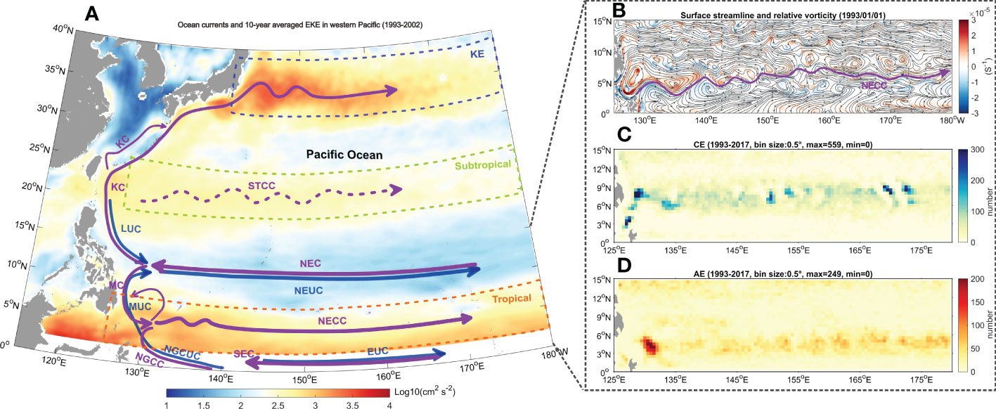
Figure 1 (A) Schematic map of the ocean circulation and 10-year averaged eddy kinetic energy (EKE, 1993–2002) based on AVISO data and three typical eddy-rich regions in the Pacific; (B) snapshot of the surface streamline, relative vorticity based on the European Copernicus Marine Environment Monitoring Service (CMEMS) datasets (1993/01/01); and the frequency statistics of all (C) cyclonic eddies (CEs) and (D) anticyclonic eddies (AEs) locations in the tropical region. The three eddy-rich regions are the Kuroshio Extension (KE), the subtropical regions, and the tropical regions, within the dotted frame in (A). The colored lines with arrows indicate the circulation pattern in the Pacific Ocean (Hu et al., 2015; Qiu et al., 2015), including the Kuroshio (KC), Luzon Undercurrent (LUC), Subtropical Counter Current (STCC), North Equatorial Current (NEC), North Equatorial Undercurrent (NEUC), Mindanao Current (MC), Mindanao Undercurrent (MUC), North Equatorial Counter Current (NECC), South Equatorial Current (SEC), Equatorial Undercurrent (EUC), New Guinea Coastal Current (NGCC), and New Guinea Coastal Undercurrent (NGCUC). The data in (C, D) are binned in 0.5°×0.5° cells for the 1993–2017 period. Note that the locations in (C, D) are centers of mesoscale eddies (MEs), and the active regions of MEs are also influenced by their size.

Previous studies have focused on the characteristics and evolution process of long-lived MEs (> 7 days) (Chelton et al., 2011a; Morrow and Le Traon, 2012; Xu et al., 2014; Faghmous et al., 2015); however, short-lived MEs have not received sufficient attention and systematic study. In previous studies, some features of short-lived MEs have been captured from the energy, frequency, surface flow field, vorticity, and other aspects in the core of the western Pacific warm pool (WPWP) (Jia et al., 2011; Chen et al., 2014; Cheng et al., 2014; Chen et al., 2015; Qiu et al., 2017b; Wang, 2017; Chen et al., 2019; Johnston et al., 2019; Qiu et al., 2019; Xu et al., 2019). The number of MEs increases as their lifetime decreases (Chelton et al., 2011a). However, the importance and environmental effects of short-lived MEs have been generally overlooked, which is partly due to the limitations of the spatial and temporal resolution of satellite altimeter data, resulting in uncertainty in determining the size and path of MEs. Yim et al. (2010) found that a spatial resolution of 1/4° may be insufficient to study MEs, and some studies have shown that observational and model data with increased spatial and temporal resolutions are beneficial to the study of MEs (Meijers et al., 2007; Yim et al., 2010). Therefore, the use of data with spatial resolution greater than or equal to 1/12° could be more beneficial for the study of short-lived MEs.

Large-scale circulations have developed in the core of the WPWP, near the North Equatorial Current (NEC), mainly between 10° and 20° N north of the equator, as well as near the South Equatorial Current (SEC), between 15° S and 4° N, and near the North Equatorial Counter Current (NECC), which is an eastward current flowing against the wind (Chen et al., 2015; Hu et al., 2015) between 3° and 10° N. The NECC is opposite to NEC and SEC, providing favorable conditions for ME development in weak Coriolis regions (south of 10° N). However, owing to the limitations of observation technology and theory cognition, short-lived MEs remain a blind area in oceanographic research, and MEs in the core of the WPWP have not garnered enough attention. Chelton et al. (2011b) also pointed out in their study that the small numbers of tracked eddies at latitudes lower than about 10° are partly attributable to technical difficulties in identifying and tracking low-latitude eddies because of noise in the SSH (sea surface height) fields and the combination of the fast propagation speeds, large spatial scales, and rapidly evolving structures of low-latitude eddies (Chelton et al., 2011b). The core of the WPWP is not only the source of material and energy transport from low to middle and high latitudes with intense air–sea interactions, but also represents the region with the most abundant precipitation (with a zonal average of 80 mg/m²/s climatically; Large and Yeager, 2009) and the most tropical cyclones developed (Peduzzi et al., 2012; Lin et al., 2013). The downstream extent (i.e., the Northwest Pacific Ocean, East Asia, and Southeast Asia, including the vast marginal seas and coastal regions) of the large-scale circulations in the core of the WPWP is spatially more extensive than that of the KE, and its potential impacts on global climate change are profound.

Therefore, the basic features, spatial-temporal variations, generation mechanisms of short-lived MEs derived from the core of the WPWP, and their potential environmental effects are studied in this work. The core of WPWP includes the warm pool in the northern and southern hemispheres; however, in this study we focus on the WPWP in the northern hemisphere and confine the core area as (0°–15° N, 125°–180° E) where there exist stronger activities of short-lived MEs (Figure S1). The data sources and methods are described in Section 2. The basic characteristics and spatial-temporal variations of short-lived MEs are described in Section 3. The generation mechanism, environmental effects and importance of the short-lived MEs are discussed in Section 4, and a summary and conclusion are presented in Section 5.

2 Materials and methods

2.1 Materials sources

Daily global ocean eddy-resolving physical reanalysis product data were produced and distributed by the European Copernicus Marine Environment Monitoring Service (CMEMS, https://resources.marine.copernicus.eu), with a high spatial resolution of 1/12°. Datasets from CMEMS have been widely used in oceanography research (Pan and Sun, 2018; Hu et al., 2019; Barnier et al., 2020; Chapman et al., 2020; Cheng et al., 2020; Chen et al., 2021). This study used the physical variables of U/V-velocity and sea surface height (SSH) from the CMEMS datasets, with the time span of 1993–2017. The study domain for cyclonic eddy (CE) and anticyclonic eddy (AE) detection was selected as (0°–15°N, 125°–180°E). The sea level anomaly (SLA), eddy kinetic energy (EKE), relative vorticity (ζ), and Rossby number (Ro) were calculated based on CMEMS datasets. The SLA was computed with respect to a 20-year mean reference period (1993–2012). The equation is given by:

$\begin{array}{ll}SLA=SSH-\overline{SSH}& (1)\end{array}$

The calculation of EKE followed Qiu et al. (2017a), which indicated the general eddy filed of EKE:

$\begin{array}{ll}EKE=\frac{1}{2}\left[\left(-\frac{g}{f}\frac{\partial h^{\prime }}{\partial y}\right)+{\left(\frac{g}{f}\frac{\partial h^{\prime }}{\partial x}\right)}^2\right]& (2)\end{array}$

where f is the Coriolis parameter, g is the gravitational constant, and h’ is the SLA. Owing to the small Coriolis force in the near-equatorial region, the results of the abnormally high EKE values are generally considered invalid, and the range of intercepted values in this study was 2°, as shown in Figure 1A.

Additionally, the relative vorticity (ζ) and Rossby number (R_o) are given by:

$\begin{array}{ll}\zeta =\frac{\partial v}{\partial x}-\frac{\delta u}{\delta y}& (3)\end{array}$

$\begin{array}{ll}Ro=\frac{\zeta }{f}& (4)\end{array}$

where u and v are the zonal and meridional components of the current velocity, respectively, and f is the Coriolis parameter.

Argo-derived mixed layer depth (MLD) data (Wu et al., 2017) (http://www.argo.org.cn/), MODIS (Moderate Resolution Imaging Spectroradiometer) Terra and Aqua Level-3 standard mapped chlorophyll-a concentration (CHL) data (Hu et al., 2012) (https://oceandata.sci.gsfc.nasa.gov/), and satellite-based time-series of sea surface temperature (SST) for climate applications as part of the European Space Agency’s Climate Change Initiative (http://data.ceda.ac.uk/neodc/esacci/sst), were also collected to study the influence of the short-lived MEs in tropical regions. Monthly ERSST (Extended Reconstructed Sea Surface Temperature) Niño 3.4 (5° N–5° S, and 170° E–120° W; 1981–2010 base period) (https://www.cpc.ncep.noaa.gov/data/indices/ersst5.nino.mth.81-10.ascii) and Pacific Decadal Oscillation (PDO, https://www.ncdc.noaa.gov/teleconnections/pdo/) data (Mantua and Hare, 2002) were also collected for analysis. The Niño 3.4 index (Niño 3.4) was used to indicate the variation of El Niño–Southern Oscillation (ENSO) phenomena. El Niño and La Niña are two opposing climate patterns in the Pacific Ocean that can affect weather worldwide, and combined, are known as the ENSO cycle (https://oceanservice.noaa.gov/facts/ninonina.html). When the absolute value of the 3-month moving average of the Niño 3.4 index reaches or exceeds 0.5°C and lasts for at least 5 months, it is considered as an El Niño event, while less than or equal to 0.5°C as a La Niña event, and others are considered as neutral phases.

Surface fluxes from NCEP/NCAR Reanalysis 1 were collected to calculated net heat flux and momentum flux (https://psl.noaa.gov/data/gridded/data.ncep.reanalysis.html). In addition, AVISO (Archiving, Validation and Interpretation of Satellite Oceanographic) (http://marine.copernicus.eu) was collected to provide SLA and the derived geostrophic current; and the EKE (Figure 1A; Figure S1) and relative vorticity (Figure S1) based on AVISO data were calculated for temporal-spatial comparison in a wider range of Pacific Ocean. The temperature profiles of the observational stations were also collected to analyze the local effect of MEs, which were obtained by Sea-Bird 911CTD in the western Pacific Ocean warm pool region. These stations were not surveyed synchronously, and the survey started on May 10, 2017 and ended on June 15, 2017, with good sea conditions and no high wind events during the survey.

2.2 Detection and tracking of MEs

Compared to the KE, the diagnosed characteristics of MEs in the core of the WPWP are not significant if only the SLA is considered. However, when the flow field is calculated and diagnosed, MEs are found to be widely distributed. Therefore, the method of Eulerian eddy detection scheme described by Nencioli et al. (2010) is adopted in this study to analyze the surface velocity geometry field, which detects the center and boundary of each eddy based on the geometric properties of the velocity vector and track its trajectory. Additionally, based on the horizontal distribution of the relative vorticity, we added a restriction on the relative vorticity to the eddy discrimination condition. The identified CE range must have positive relative vorticity and the AE range must have negative relative vorticity. The velocity field used in the study was the output of CMEMS dataset, with the time span of 1993–2017 and the domain for eddy detection of (0°–15°N, 125°–180°E). The boundary of an eddy is defined as the contour closed by the maximum velocity around the center point of the eddy.

The tracking range is determined based on the resolution and distribution of the flow field (Nencioli et al., 2010; Zhang et al., 2018). A single eddy track is first recorded as an eddy detected at t moment in the domain, i.e. an eddy is generated, then we search for the eddy with the same polarity within the searching range of R=14 grid points at time t+1 moment, and select the closest eddy among them (Nencioli et al., 2010). If no matching eddy is found in the given area of R at given time t+1, an enlarged searching range of 1.5 times the R at time t+2 moment is performed for continuously searching. Information on different aspects of MEs, including the polarity, location, boundary, and lifespan, can be identified according to this method, which has been widely used in previous studies (Dong et al., 2012; Liu et al., 2012; Dong et al., 2014; Lin et al., 2015; Liu et al., 2017a; Zhang et al., 2018).

3 Results

3.1 Basic features of MEs

The basic features of the MEs were analyzed based on the detected properties of the CEs and AEs (Figure 2). The MEs with coherent structures developed in the core of the WPWP were mainly short-lived eddies with lifespans of less than 7 days (Figure 2A). The lifetime of an eddy is defined as the time interval between the first record and the final record in a single track. The number of CEs (AEs) with a lifespan of less than 7 days accounted for 96.07% (95.54%). The ratios of CE and AE lifespan distributions were approximately identical, and the proportion of long-lived MEs greater than 7 days in this region was very small. The radii of the equal-area circles with MEs were mainly between 50 and 200 km (Figure 2B), which is similar to the magnitude of long-lived MEs (not shown). The ratio of AEs with large radii (larger than 1.5°) were relatively larger than that of CEs (Figure 2B), the averaged radius of AEs is 1.20°, which is larger than that of CEs (1.08°). The relative vorticity at the eddy center and the maximum SLA within the CE and AE showed a symmetrical distribution (Figures 2C, D). The relative vorticity ranged from −20×10^-6 to 20×10^-6 s^-1, and the CE (AE) was positive (negative). The SLA, calculated using the equation (1), was mainly distributed between −40 and 40 cm, and the CE (AE) was negatively (positively) biased owing to the divergence (convergence) of seawater caused by the CE (AE). The maximum rotation speed within the eddy region was mainly distributed between 0.2 and 0.8 m/s (Figure 2E). The propagation speed (Figure 2F) of an eddy refers to the average velocity of the eddy’s center along the motion route during the life cycle (t days, t ≥ 2), and the propagation speed of MEs was mainly between 0.1 to 1 m/s (Figure 2F). Figures 2G–I show the statistical characteristics of the ellipse with the same standard second-order central moment as that of the MEs. Here, the eccentricity (Figure 2G) was mainly distributed between 0.5 and 1, and the length of the long axis (Figure 2H) was between 100 and 700 km, whereas that of the short axis (Figure 2I) was between 50 and 400 km.

FIGURE 2

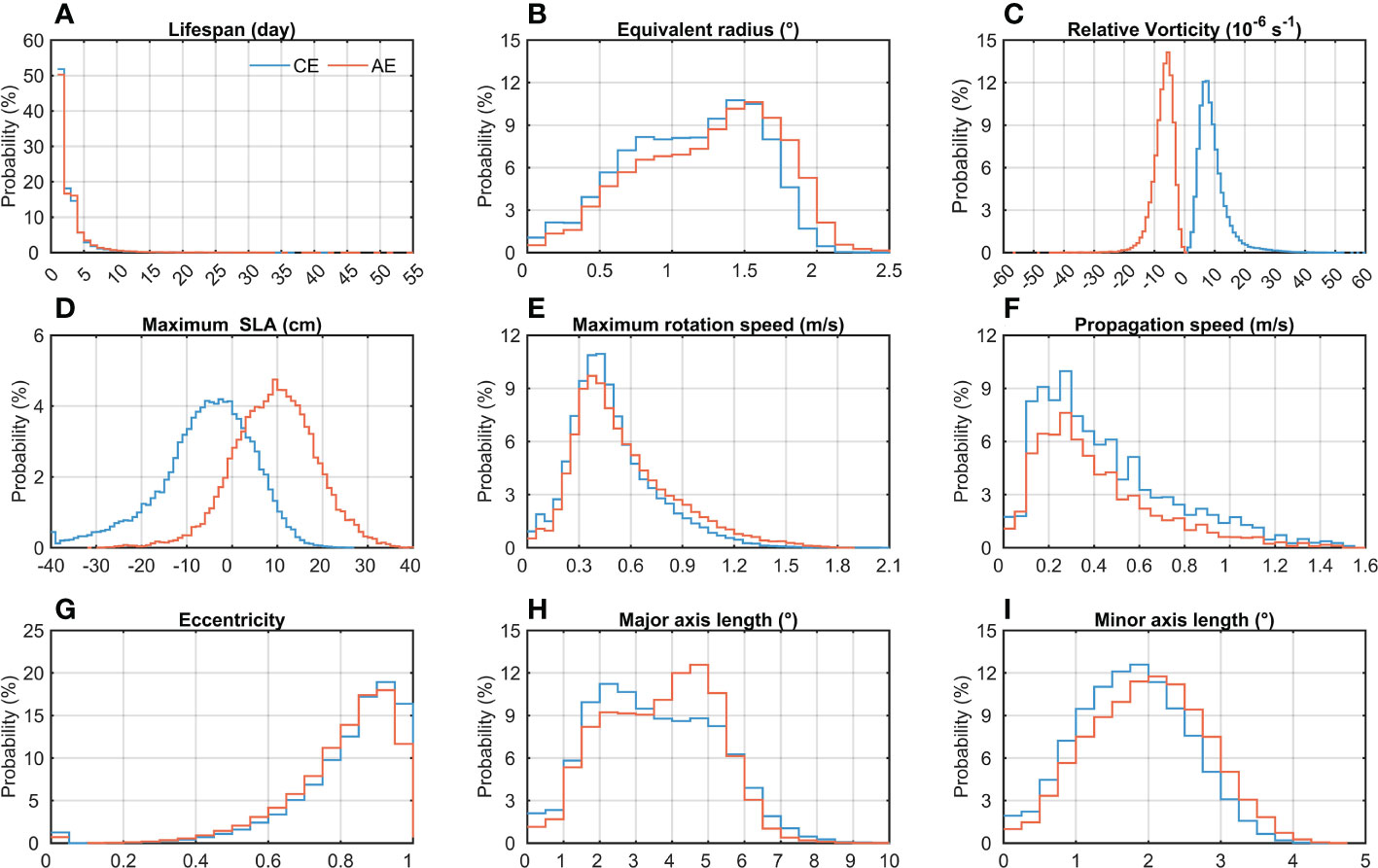
Figure 2 Basic features of the MEs in the core of the western Pacific warm pool (WPWP). The blue and red lines represent CE and AE in (A–I). The variables in (D, E) are maximum values within the region of the detected MEs, and the relative vorticity (C) is the value at the centers of MEs. The variables shown in (B, G–I) are corresponding variables of an ellipse with the same standard second order central moment as the region of an eddy, i.e. the equivalent radius, eccentricity, major axis length, and minor axis length of the ellipse.

3.2 Spatial variations of MEs

Based on the spatial distributions of the surface streamline and relative vorticity, MEs were extensively developed in this tropical region (Figure 1B; Video S1). CE (AE) had a positive (negative) relative vorticity and was spatially characterized by a cold (warm) eddy. The tropical eddy-rich region had a large EKE (Figure 1A). According to the frequency statistics of all CE and AE locations in the core of the WPWP (Figures 1C, D), the CE and AE had significant spatial band-like characteristics. CEs were mainly distributed between 5° and 9° N with a central axis at 8°N, located between NEC in the north and NECC in the south, while AEs were mainly distributed between 3° and 5°N with a central axis at 4°N, located between NECC in the north and SEC and NGCC in the south (Figure 1). The locations of ME belts varied over time (Figures 3A, B) and were affected by the meridional fluctuations of the NECC. The number of MEs increased sharply at the turn of the circulation near the coast (Figures 1C, D), corresponding to the positions of the Mindanao and Halmahera eddies in previous studies (Kashino et al., 2013; Chen et al., 2014; Qiu et al., 2015; Liu et al., 2017b).

FIGURE 3

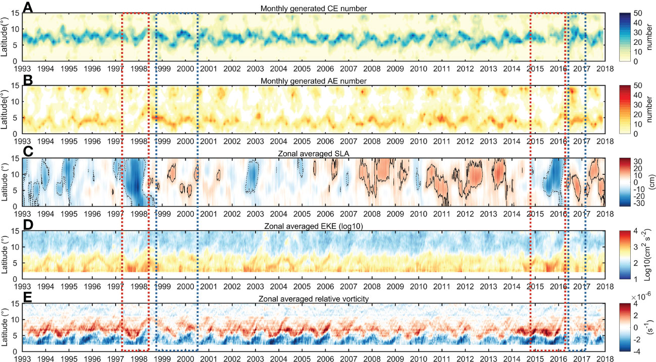
Figure 3 Time series of (A, B) the monthly generated ME number at different latitudes, and (C) zonal-averaged SLA, (D) EKE (log10), and (E) relative vorticity from 1993–2017. The black dotted (solid) line in c represents the SLA contour line of –10 cm (10 cm). The calculation is zonal-averaged from 125°–180°E. The red and blue frames indicate two strong El Niño (1997 and 2015) and La Niña phases (1999 and 2016), respectively.

The spatial−temporal variation of the zonal-averaged SLA in the tropical eddy-rich region is shown in Figure 3C. During the El Niño phase (Figures 3, 4H), there was a negative anomaly (< −10 cm), whereas the La Niña phase showed a positive anomaly (> 10 cm). During the neutral phase, the SLA was between −10 and 10 cm. The EKE regions with high values were distributed between 2° and 10° N (Figures 1A and 3D), which was consistent with the spatial distribution of the CE and AE belts (Figures 1C, D, 3A, 3B). During the El Niño phase, the region of high EKE moved southward and the area with high values was reduced, but the intensity increased, especially during the strong E1 Niño period (1997/1998 and 2015/2016). Note that EKE is not completely consistent with the number of MEs, but is also related to the size, intensity of MEs, and even background current field, in which the non-coherent eddy field such as meanders, filaments and fronts contribute a lot. The location and number of MEs are relatively discrete, which can better represent the overall spatial and temporal variation of MEs in this tropical region, respectively. According to the current velocity distribution, the circulation in this region was zonally distributed, and the two belts were distributed on both sides of the NECC. The regularity of the spatial difference distribution of the eddy belts was also significant from the perspective of relative vorticity (Figure 3E), and the CE (AE) belt was positive (negative), which is consistent with the statistical characteristics shown in Figure 2C and Figure S2.

FIGURE 4

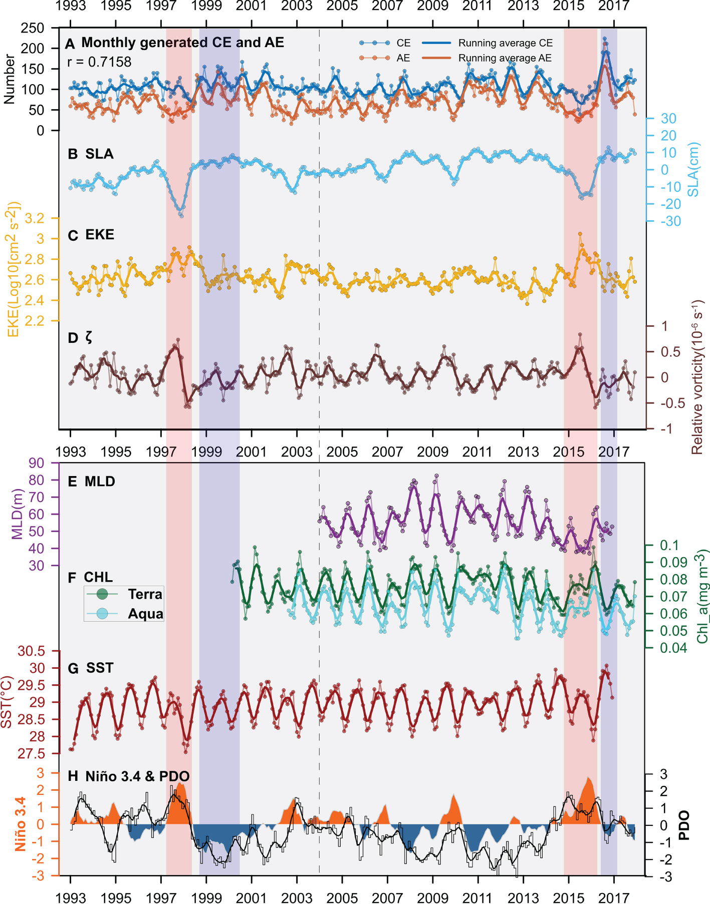
Figure 4 Time series of the monthly generated numbers of (A) CEs and AEs, monthly regional averaged (B) SLA, (C) EKE (log10), (D) relative vorticity (ζ) in the area of (2°–10° N, 125°–180° E) for the 1993–2017 period, and monthly regional averaged (E) Argo-derived mixed layer depth (MLD), (F) chlorophyll-a (CHL) concentration, (G) sea surface temperature (SST) in the area of (0°–15° N, 125°–180° E), and (H) Niño 3.4 and PDO indices. The dotted lines in (A–G) show the original data and the bold lines indicate 5-step moving-averaged data. The color patches in (H) represent the Niño 3.4 index, while the black lines represent the PDO index with the thin black and thick black lines indicating the original data and 5-step moving-averaged data, respectively. The red and blue shaded areas indicate two strong El Niño and La Niña phases, respectively.

3.3 Temporal variations of MEs

An average of 108.00 CEs and 71.42 AEs were generated in the tropical eddy-rich region every month. The number of CEs was generally greater than that of AEs, and they showed synchronous temporal variations, with a correlation of 0.72 (Figures 4A). The development of MEs was characterized by interannual and seasonal fluctuations. The number of CEs was higher in the second half of the year (July–December) and lower in the first half (January–June) (Figure 5A). Meanwhile, the number of AEs was higher from April to September, and lower in the other months. The fluctuation range of the number of MEs in the second half of the year was larger than that in the first half (Figure 5A). Both CEs and AEs number have higher numbers in summer and lower in winter (Figure 5A). During El Niño, the WPWP was in the relatively cold phase, the amounts of CEs and AEs were significantly reduced, and the decrease in AEs was greater than that of CEs, especially during the strong El Niño phase when both the PDO and Niño 3.4 were in the positive phase (Figures 4A, H, 5B, D). During the La Niña phase, the WPWP was in a relatively warm phase, and the amounts of CEs and AEs increased significantly, and the increase in AEs was greater than that of CEs (Figures 4A, H, 5C, E). During the neutral phase, the anomalous amounts of CEs and AEs showed little difference around the zero value (Figure 5F). The number of AEs was more variable and sensitive to changes in the ENSO index (Niño 3.4) than that of CEs (Figures 4H, 5D, E).

FIGURE 5

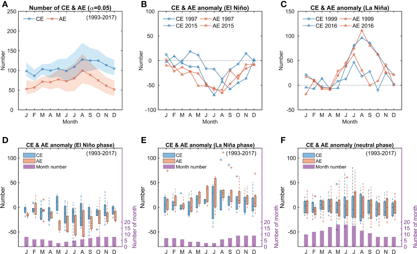
Figure 5 Monthly generated number of MEs. (A) The average value and 95% confidence interval of CEs and AEs (significance level (α) of 0.05); (B, C) the anomalies of the number of MEs during strong El Niño (1997 and 2015) and La Niña (1999 and 2016) phases; (D–F) the multi-year averaged anomalies of the number of MEs and the number of month during El Niño, La Niña and neutral phases (right axis); the vertical dashed lines indicate the distribution range of the normal value of this set of data, the plus markers are classified as outliers, the shaded bars indicate the interquartile range, and the black lines in the bars are the median values.

Sea level anomaly changes were significant in response to the E1 Niño signals (Figures 3C, 4B, H). The EKE, current velocity, and relative vorticity all showed high values during the low SLA periods (Figures 4B-D). During the strong El Niño phase, the number of CEs and AEs decreased, and SLA showed a significant negative anomaly. The results of SLA, EKE, and relative vorticity based on CMEMS data were mostly consistent with those based on AVISO data in this tropical eddy-rich region (Figures 3 and Figure S2).

In addition, the changes in the MLD, CHL, and SST in the core region of the WPWP had obvious seasonal and interannual patterns (Figure 4). Based on the MLD products derived from the Argo data, the average monthly MLD in this region was approximately 57.36 m (2004–2016), which was relatively shallow, with a fluctuation range of 30–90 m (Figure 4E). The surface CHL concentrations fluctuated consistently with the MLD at temporal scale, with a recorded average of approximately 0.08 mg/m³ estimated from MODIS Terra (2000–2017, Figure 4F) and 0.07 mg/m³ estimated from MODIS Aqua (2002–2017, Figure 4F). The standard deviations of the two datasets are 0.0097 mg/m³ for Terra and 0.0101 mg/m³ for Aqua. The WPWP is one of the warmest parts of the global ocean, with an average monthly temperature of 28.93°C (1993–2016) in the core region (Figure 4G), and the SST was positively correlated with the development of the MEs. See Section 4.2.1 for a detailed analysis.

4 Discussion

4.1 Generation mechanism of MEs

The dynamic mechanism of ME generation is relatively complex, and previous studies have suggested that the occurrence frequencies of MEs are affected by multiple mechanisms, such as the circulation instability (e.g., horizontal shear, vertical shear) and density frontal instability, gravitational potential energy storage, interaction of the ocean current with the bottom topography, vorticity conservation, and wind forcing (Chelton et al., 2011a; Morrow and Le Traon, 2012; Cheng et al., 2013; Rhines, 2019; Xu et al., 2019; Wang et al., 2021). Combined with the distribution of the AE and CE belts (Figures 1C, D, 3A, B), the U and V components of the current (Figures 6A, B), and relative vorticity (Figure 3E), and the time series of SST and its gradient, it was found that MEs in this region are mainly generated by the shear instability of large-scale ocean currents, and are influenced by climate signals such as the PDO and ENSO (Figure 4), the shear instability is closely related to baroclinic instability in the core region of WPWP, and the horizontal shear and vertical shear are actually not independent in the background flow field. Baroclinic instability can be viewed as a shear instability (Grotjahn, 2003). The baroclinic instability could occur when meridional temperature gradients change of sign. The baroclinic instability caused by variations of meridional SST gradients controls the variation patterns of MEs number (Figure 7). The results of the power spectra of SST, SST gradient, and the number of CE/AE also reveal the significant semiannual and annual period signals (Figure S3). The mean meridional gradient of SST (dSST/dy) and the detrended SST shows a positive correlation with a coefficient of 0.70 (Figure 7F). As the SST of the WPWP increases, the SST gradient increases, and the shear instability also strengthen, thus CEs and AEs are more likely to be generated (Figures 7A–D), and the patterns of positive baroclinic instability at AE belt is more obvious than that at CE belt (Figure 7E). Conversely, when the SST decreases, the shear instability weaken, and the number of CE/AE is reduced.

FIGURE 6

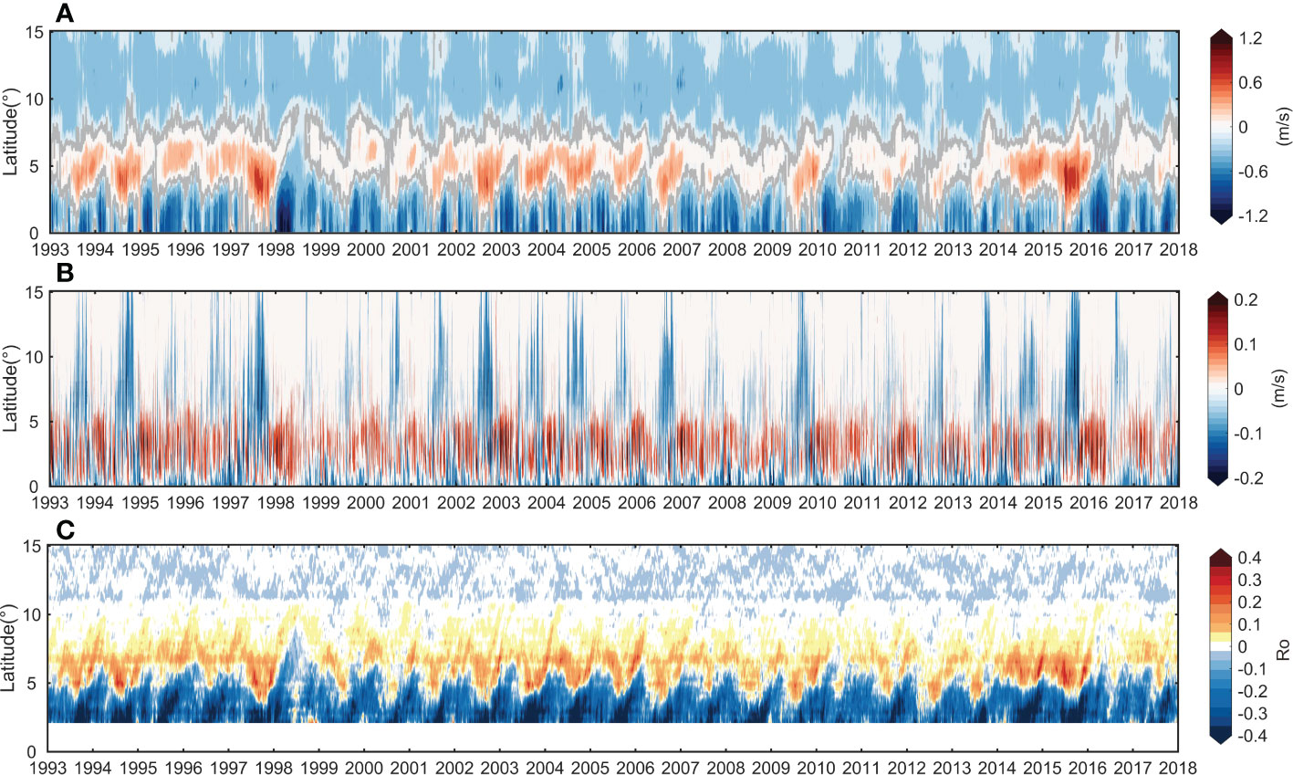
Figure 6 Time series of the zonal-averaged (A) U and (B) V components of the background current velocity, and (C) Rossby number (Ro) for the 1993–2017 period. The gray lines in (A) show the contour of zero value. The U/V-velocity in this plot is derived from the variables of CMEMS data.

FIGURE 7

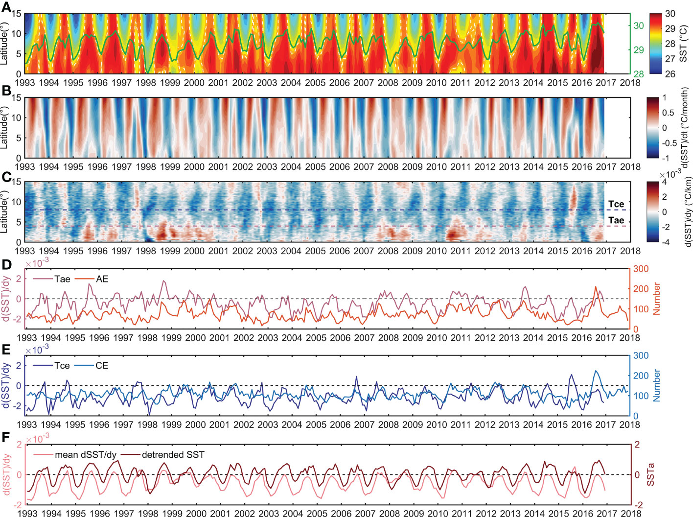
Figure 7 Time series of the zonal-averaged (A) SST, (B, C) temporal and meridional gradients of SST, (D, E) comparison of typical transects (eddy belt region) of SST gradients and ME number, and (F) comparison of the mean meridional gradients of the SST and the detrended SST in this tropical region. The green line in (A) indicates the average value of [0°–7.5° N; 125°–180° E], and white dash line indicates the contour of 28.93°C. The transects Tae and Tce in (C–E) indicate the meridional gradients of SST in CE and AE belts, respectively.

According to the zonal-averaged Rossby number, this tropical region could still be influenced by planetary rotation (Figure 6C). However, considering that the Coriolis forcing near the equator is relatively small and the geostrophic equilibrium is unstable, it is inadequate to maintain the development and movement of MEs in a long-term stable state. The fluctuation of the local flow field and relative vorticity are high; thus, MEs are easily generated or dissipated, which is different from other eddy-rich regions, such as the KE and subtropical regions (Video S1). The meridional and temporal gradients of the relative vorticity and the U and V components of the current velocity also showed higher variation rates at lower latitudes, which is characteristic of high-frequency turbulence in this region (Figure S4). In addition, the ocean currents steer near the land and the current shear is strong in this region; thus, many MEs are developed near the coastline (Figures 1C, D).

4.2 Environmental effects analysis

4.2.1 Regulation effects of MEs on SST in tropical region

The year-round SST in the area of WPWP is very high (Figures 4G, S5A, B), and the warm water in the MLD is mainly located in the upper layer of the tropical ocean (Figures S5C, D). As discussed in Section 4.1, the variations in SST could influence the generation of MEs, thus the empirical orthogonal function (EOF) for SST and detail analysis of temperature profiles were performed.

The four leading EOF modes of the SST are shown in Figures S6. The time series of the four EOF modes are shown in Figures S6B, D, F, H. Their contributions to the total variance were 40.73%, 30.05%, 7.68%, and 3.97%, respectively, accounting for 82.43% of the total variance altogether. The ENSO signal and short-lived eddies were found to be two important factors contributing to those variations (Figure 8). Mode 1 shows the ENSO cycle of the SST in this region. During El Niño phase, the SST in this region was much smaller than that during the La Niña phase. This pattern was generally in coherence with the annual variation of Niño 3.4, while in opposite with the low-frequency signal of the short-lived eddies (Figure 8C), the eddy variability is also characterized by long time cycles. Besides, the results also show that the spatial pattern of the third mode (EOF3) displays a latitudinal band distribution (Figure S6E), which is consistent with the distribution of eddy belts, and the spatial pattern of the fourth mode (EOF4) shows a meridional distribution (Figure S6G). Moreover, on the time scale, the high-frequency SST mode (PC3+PC4, the sum of the third and fourth modes) matches well with the high-frequency signal of the short-lived eddies (Figure 8D).

FIGURE 8

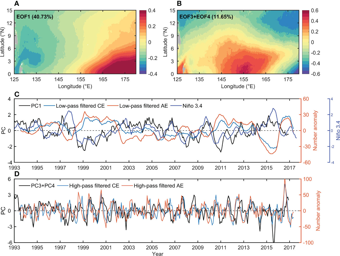
Figure 8 Empirical orthogonal function (EOF) for SST (1993–2016) in western Pacific warm pool region and comparison of different modes with MEs. (A, B) The EOF mode 1, the sum of modes 3 and 4 for SST, and (C, D) their corresponding PC time series. The percentage of variance explained by each mode is displayed in the upper-left corner of each EOF panel. The PC time series from top to bottom are superimposed on the low-pass filtered eddy numbers, Niño 3.4 index (C), and high-pass filtered eddy numbers (D). See Figure S6 for original EOF results.

Based on the observational results of temperature profiles, the short-lived eddies could effectively regulate the vertical temperature structures in the water columns (Figure 9). By comparing the observational temperature profiles inside and outside the eddy regions at the same latitude, it can be seen that the upwellings inside the CEs have a greater influence on the internal temperature of the eddies, and for the same depth, the eddy-influenced water column can be cooled by approximately 3°C. The AE can also significantly affect the temperature structure inside the eddy region through downwelling, the temperature of eddy-influenced water column above 35 m dropped by approximately 0.7°C, then affecting the SST, meanwhile, the water temperature between 35 m and 78 m water depth increased by approximately 1.4°C. The observational results could qualitatively indicate that eddies affect the redistribution of heat in the water column through the upwelling and downwelling processes.

FIGURE 9

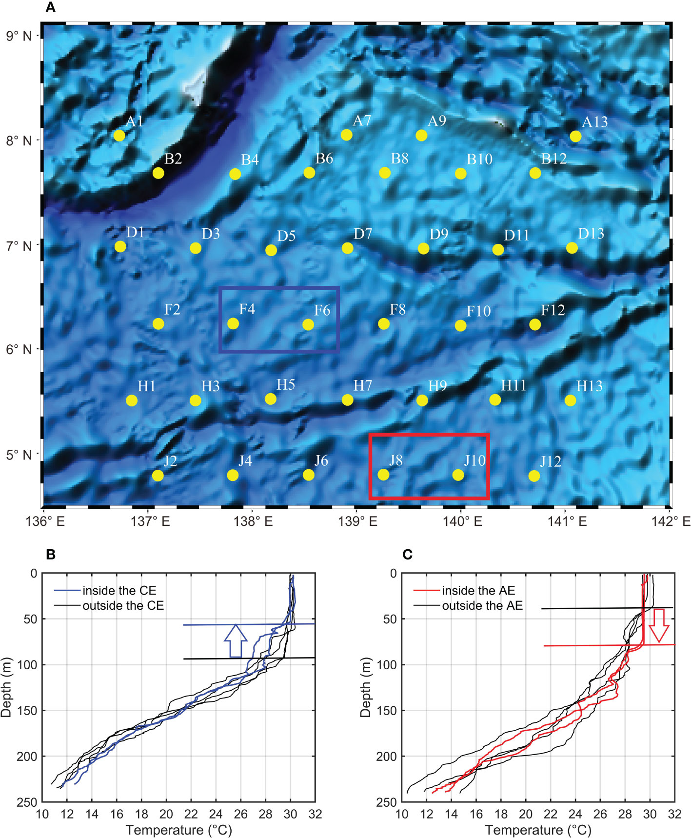
Figure 9 The temperature profiles of the observational stations, (A) is station distribution map, in which the blue and red boxes represent location of stations within the eddy ranges, respectively; (B) temperature profiles of stations inside two different CEs and other stations at transect F with the same latitude; (C) temperature profiles of stations inside a single AE and other stations at transect J with the same latitude.

Besides, through the linear regression fitting between the abnormal number of monthly generated CEs and AEs and monthly mean SSTa in the eddy belts region (Figure 10A), the results showed that both have significantly positive correlation, with correlation coefficients of 0.47 and 0.31, respectively. The seasonal fluctuations of ME number, net heat flux (Q_n), and momentum flux at surface are basically consistent with each other (Figure S7), specially the net heat flux at two eddy belts are obviously different, the generation and disappearance of short-lived MEs developed in the eddy belts may also affect the heat flux exchange at air–sea interface and momentum flux in this near-equatorial region, these processes could also regulate SST in the WPWP (Figure S7).

FIGURE 10

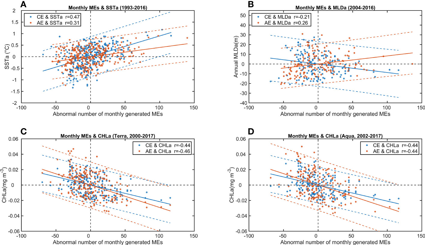
Figure 10 Linear regression fitting between abnormal number of monthly generated MEs (CEs and AEs) number and monthly (A) SSTa, (B) MLD anomalies (MLDa), (C) CHL anomalies (CHLa, Terra), and (D) CHLa (Aqua). The correlation coefficients are labeled in the subfigures.

Based on the structures of local flow fields and variations of SST and SST gradient in the core region of WPWP (Figures 1B, 6A, B, 7A–C, Video S1), it could be noticed that the associated circulations around the CEs could transport the slightly warm water from the south of the eddy region away from the equator, and transport the slightly cold water from the north of the eddy region close to the equator, respectively. Similarly, the associated circulations around the AEs could also play the same roles in the southern side of NECC. Therefore, the generation and disappearance of CEs/AEs could influence the redistribution of heat in vertical and horizontal scales, which is the regulation process of SST in the core region of WPWP. The associated circulations around the CEs and AEs could play the role of convergence/divergence of meridional heat transport, which could carry the relatively cold water toward the equator and warm water away from the equator, a model diagram was posed to show this regulation process of MEs on the SST of WPWP (Figure 11). Although the SST of the WPWP is generally in a high level, this process could become stronger when the SST is higher (positive SSTa), and weaker when the SST is lower (negative SSTa, Figure 10A).

FIGURE 11

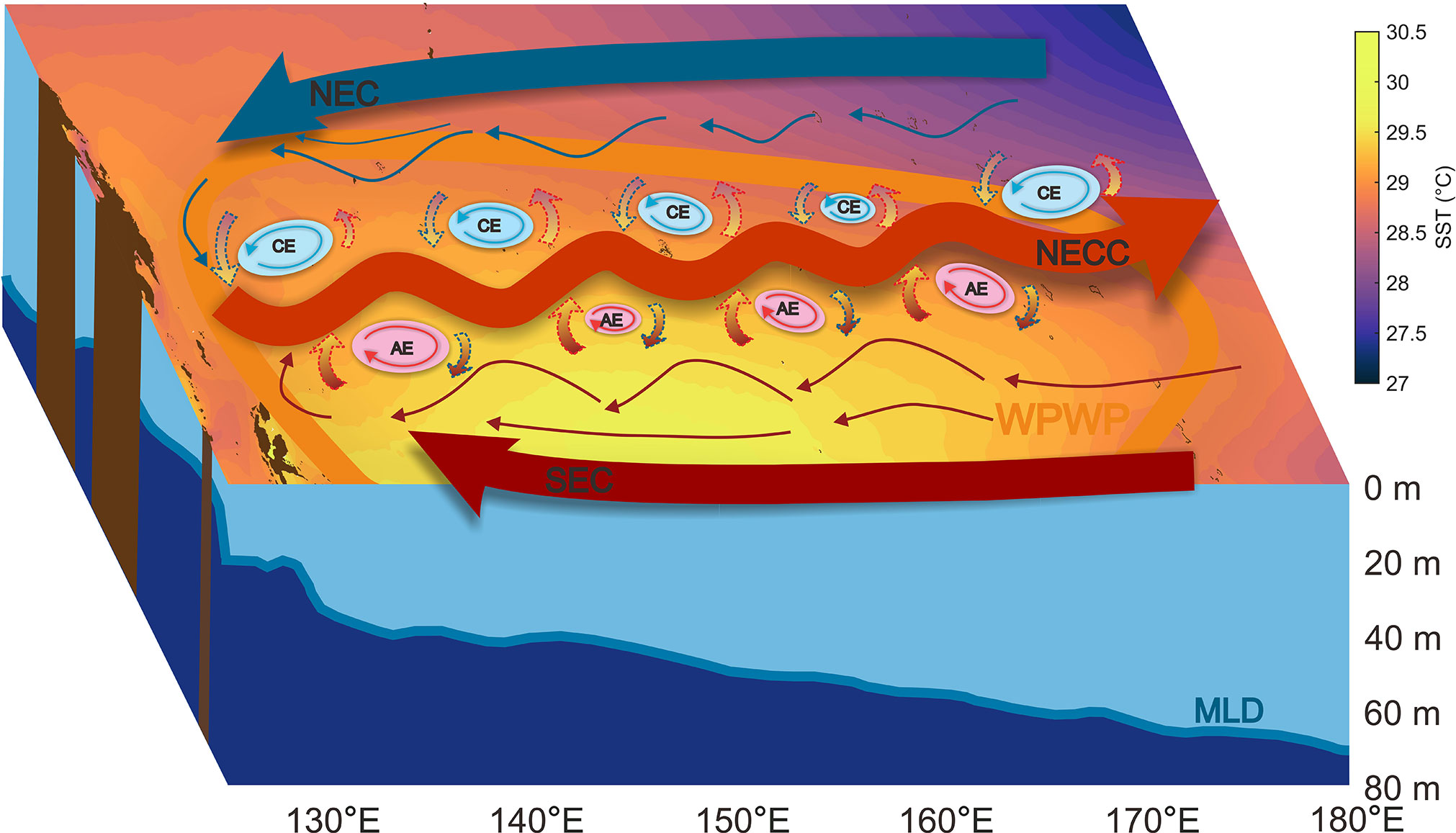
Figure 11 Model diagram of short-lived MEs regulating the western Pacific warm pool region.

To sum up, the short-lived MEs in this tropical region helps to regulate the redistribution of heat between large-scale circulations, by transporting slightly warm (cold) water away from (close to) the equator through the associated circulations around the MEs. The two eddy belts connect the large-scale circulations in terms of spatial dynamic patterns and heat transfer, which could further influence other areas in the ocean through large-scale circulations such as the western boundary currents. We figure that in addition to the important role of the MEs in heat transport, the heat transport brought by the eddy induced flow field of the surrounding sea area should not be neglected, which may also play an important role in heat redistribution in the sea area where the MEs develop with a short life cycle or short moving distance.

4.2.2 Regulation effects of MEs on MLD/CHL in tropical region

Similarly, the relationship between the MEs and MLD, CHL were studied in this section. Although the variations in SST and MLD are probably dominated by large-scale ocean circulations and sea surface heat fluxes (Figures S5, S7), they are also regulated by MEs. The temporal and meridional averaged SST and MLD (Figures S5B, D) show meridional differences, especially a secondary peak value of MLD can be found around the 5° N (Figure S5D), possibly indicating the MLD is closely related to both the circulation structure and short-lived MEs in the near-equatorial region. Compared to SST, the MLD shows more obvious fluctuations at the region where short-lived MEs developed. Therefore, the development of short-lived MEs also accelerates the adjustment of MLD in the tropical region of the banded eddy area.

From the measured CTD profiles and the statistical results, it can be seen that the regulation effects of the mixed layer by CEs and AEs are opposite, with CEs being detrimental to the deepening of the mixed layer and AEs being beneficial to the deepening of the mixed layer (Kouketsu et al., 2012; Gaube et al., 2013; Dufois et al., 2014; McGillicuddy, 2016) (Figures 9B, C and 10B). The upwelling of isopycnals inside CE could result in shallower MLD during its formation and intensification stages, from approximately 92 m to 54 m, and downwelling of isopycnals inside AE could result in a deeper MLD, from approximately 35 m to 78 m (Figures 9B, C). The correlation analysis results show that the abnormal number of monthly generated MEs and the MLDa are weakly correlated, with the CEs/AEs being able to influence the MLD of the corresponding eddy belts, but not being the dominant factor. The heat exchange at the air-sea interface and wind stress should be the dominant factor controlling the seasonal cycle of the MLD, as well as the SST and CHL (Kara et al., 2000; Kara et al., 2003; Kouketsu et al., 2012).

Besides, the relationship between the abnormal number of monthly generated CEs and AEs and CHL anomalies (CHLa) shows an obvious negative correlation (Figures 10C, D). Both MODIS Terra and MODIS Aqua datasets are compared, and the results are nearly the same, indicating that the influence of CEs and AEs on the change in CHL in the surface layer was presented in antiphase, which was consistent with the results shown in the time series in Figures 4A, E, F; that is, the temporal variations of MEs were not synchronous with that of CHL (Figures 4A, F); however, the temporal variations of MLD and CHL were almost the same (Figures 4E, F and S8). Previous studies found that the mechanisms by which MEs influence CHL fundamentally rest on the delivery of nutrients, which can be divided into eddy advection (Chelton et al., 2011b; Siegel et al., 2011), eddy stirring and trapping of CHL (Chelton et al., 2011a; Lehahn et al., 2011; Gaube et al., 2014), eddy-induced Ekman pumping (McGillicuddy et al., 2007; Gaube et al., 2013; Gaube et al., 2015; Xu et al., 2019), and eddy strain-induced pumping (Zhang et al., 2019; Zhang & Qiu, 2020). In addition, surface eddy-induced Ekman pumping may be the most effective mechanism for AEs in upper-ocean nutrient enrichment, by continuously supporting injection of nutrients in the center of eddies (Chen et al., 2020). For the CHL at two eddy belts in this study, they are close to synchronous variation, with a correlation coefficient of 0.89 (Figure S9), which is probably due to the effect of advective transport caused by eddies (Chelton et al., 2011a), through transporting relatively high CHL water from near equator to the north and transporting low CHL water from the north side to the south, thus relatively high concentrations of water are diluted.

Objectively, this study clearly shows that the short-lived MEs could influence the SST, MLD and CHL in the core region of the WPWP at different spatial-temporal scales, but the efficiency of the MEs influencing the SST/MLD/CHL and the mechanism of the ecological effect need further exploration through high-resolution numerical model and long-term observations. Furthermore, the WPWP acts as one of the most important warm poles on the Earth, and is a region where tropical cyclones are widely developed. Short-lived MEs could probably therefore affect the global climate change by adjusting the SST and MLD of the WPWP, and their potential impacts on extreme weather events also require further study.

5 Summary and conclusions

Stable ME belts in the core of the WPWP were diagnosed and extracted for the first time based on high-resolution flow-field CMEMS data. The eddy belts were characterized by short-lived CEs and AEs in the tropical region. The ratios of CEs and AEs with lifespans shorter than 7 days were 96.07% and 95.54%, respectively. The radii of an equal-area circles with MEs ranged from 50 to 200 km, which is similar to that of long-lived MEs. The maximum SLA of CEs and AEs were distributed symmetrically. The CE (AE) was characterized by a cold (warm) eddy and a positive (negative) relative vorticity. The CE and AE belts were distributed on the northern and southern sides of the NECC, respectively, with significant differences in spatial distribution, and this tropical eddy-rich region had a high EKE. The CEs and AEs showed synchronous temporal variations, and the development of MEs showed interannual and seasonal fluctuations. CEs (AEs) were generated more frequently from July to December (April to September) and were affected by the ENSO signals. During the El Niño periods, the WPWP was in the cold phase, when the generation of CEs and AEs decreased, and the number of AEs decreased more than that of the CEs. In contrast, the WPWP was in the warm phase during La Niña, and the number of CEs and AEs increased significantly.

The CEs and AEs were mainly formed by the shear instability of the large-scale circulations, namely NECC, NEC, SEC, and NGCC, respectively, and are influenced by climate signals such as the PDO and ENSO. The shear instability is closely related to baroclinic instability in the core region of WPWP. The baroclinic instability caused by the variation of SST gradient controls the variation of ME number.

In addition, the development of MEs in the core region of the WPWP can regulate the redistribution of heat between large-scale circulations, by transporting slightly warm (cold) water away from (close to) the equator through the associated circulations around the MEs, which could further influence other areas in the ocean through large-scale circulations. The regulation effects of the mixed layer by CEs and AEs are opposite, with CEs being detrimental to the deepening of the mixed layer and AEs being beneficial to the deepening of the mixed layer. The abnormal number of monthly generated MEs and the MLDa are weakly correlated, while the relationship between the abnormal number of monthly generated CEs and AEs and CHLa shows a negative correlation.

The short-lived MEs could influence the SST, MLD, and CHL structures in the core region of the WPWP. These results reveal that short-lived MEs in the WPWP are significant supplements to understanding long-lived and long-distance propagated MEs, combined with previous research. This study can provide new perspectives and target areas for future research on global ocean eddies, and fill a gap in the study of low-latitude ocean eddies. Moreover, it is necessary to further explore the contribution of short-lived MEs to the transport and exchange of matter and energy and their roles in tropical cyclone formation, as well as to re-examine their potential impacts on global air–sea interactions and climate change, this will be further explored in future studies.

Data availability statement

The original contributions presented in the study are included in the article/Supplementary Material. Further inquiries can be directed to the corresponding authors.

Author contributions

ShL: Methodology, Investigation, Data curation, Conceptualization, Writing-original draft, Writing-review and editing. JX: Conceptualization, Investigation, Validation, Supervision. LQ: Conceptualization, Methodology, Writing-review and editing, Supervision. GL: Conceptualization, Methodology, Writing-review and editing, Supervision. JS: Resources. DD: Resources, Supervision. DY: Resources. XY: Resources. YP: Resources. SiL: Resources. XF: Resources, Figure editing. All authors contributed to the article and approved the submitted version.

Funding

This study was jointly supported by the National Natural Science Foundation of China (grant No. 41806072, 42076179, 41976198, 41030856, 41476030), the Project of Taishan Scholar grant to GL, National Key R&D Program of China (grant No. 2017YFE0133500), National Program on Global Change and Air-Sea Interaction (grant No. GASI-02-PAC-CJ15), the Fundamental Research Funds for the Central Universities (grant No. 202172003), and the project funded by China Postdoctoral Science Foundation (grant No. 2019M652467) and Qingdao postdoctoral application research.

Acknowledgments

We thank professor Changming Dong from Nanjing University of Information Science and Technology for his lectures on the second SODE Starfish Open Course supported by the State Key Laboratory of Satellite Marine Environmental Dynamics, Second Institute of Oceanography, Ministry of Natural Resources. We thank Dr. Zhigang Yao for his help in the analysis of the study, and Xiao Liu for her advice in preparing the figure. We are grateful to all reviewers for their constructive comments and suggestions, which are helpful to the improvement of this work.

Conflict of interest

JS and XF are employed by Qingdao Blue Earth Big Data Technology Company Limited.

The remaining authors declare that the research was conducted in the absence of any commercial or financial relationships that could be construed as a potential conflict of interest.

Publisher’s note

All claims expressed in this article are solely those of the authors and do not necessarily represent those of their affiliated organizations, or those of the publisher, the editors and the reviewers. Any product that may be evaluated in this article, or claim that may be made by its manufacturer, is not guaranteed or endorsed by the publisher.

Supplementary material

The Supplementary Material for this article can be found online at: https://www.frontiersin.org/articles/10.3389/fmars.2023.1069897/full#supplementary-material

References

Barnier B., Domina A., Gulev S., Molines J.-M., Maitre T., Penduff T., et al. (2020). Modelling the impact of flow-driven turbine power plants on great wind-driven ocean currents and the assessment of their energy potential. Nat. Energy 5 (3), 240–249. doi: 10.1038/s41560-020-0580-2

CrossRef Full Text | Google Scholar

Chapman C. C., Lea M. A., Meyer A., Sallee J. B., Hindell M. (2020). Defining southern ocean fronts and their influence on biological and physical processes in a changing climate. Nat. Climate Change 10 (3), 209–219. doi: 10.1038/s41558-020-0705-4

CrossRef Full Text | Google Scholar

Chelton D. B., Gaube P., Schlax M. G., Early J. J., Samelson R. M. (2011a). The influence of nonlinear mesoscale eddies on near-surface oceanic chlorophyll. Science 334 (6054), 328–332. doi: 10.1126/science.1208897

PubMed Abstract | CrossRef Full Text | Google Scholar

Chelton D. B., Schlax M. G., Samelson R. M. (2011b). Global observations of nonlinear mesoscale eddies. Prog. Oceanogr. 91 (2), 167–216. doi: 10.1016/j.pocean.2011.01.002

CrossRef Full Text | Google Scholar

Chen G., Chen X., Huang B. (2021). Independent eddy identification with profiling argo as calibrated by altimetry. J. Geophys. Res.: Oceans 126 (1), e2020JC016729. doi: 10.1029/2020JC016729

CrossRef Full Text | Google Scholar

Chen K., Gaube P., Pallàs-Sanz E. (2020). On the vertical velocity and nutrient delivery in warm core rings. J. Phys. Oceanogr. 50 (6), 1557–1582. doi: 10.1175/jpo-d-19-0239.1

CrossRef Full Text | Google Scholar

Cheng Y. H., Chang M. H., Ko D. S., Jan S., Andres M., Kirincich A., et al. (2020). Submesoscale eddy and frontal instabilities in the kuroshio interacting with a cape south of Taiwan. J. Geophys. Res.: Oceans 125 (5). doi: 10.1029/2020jc016123

CrossRef Full Text | Google Scholar

Cheng Y.-H., Ho C.-R., Zheng Q., Kuo N.-J. (2014). Statistical characteristics of mesoscale eddies in the north pacific derived from satellite altimetry. Remote Sens. 6 (6), 5164–5183. doi: 10.3390/rs6065164

CrossRef Full Text | Google Scholar

Cheng X., Xie S.-P., McCreary J. P., Qi Y., Du Y. (2013). Intraseasonal variability of sea surface height in the bay of Bengal. J. Geophys. Res.: Oceans 118 (2), 816–830. doi: 10.1002/jgrc.20075

CrossRef Full Text | Google Scholar

Chen G., Han G., Yang X. (2019). On the intrinsic shape of oceanic eddies derived from satellite altimetry. Remote Sens. Environ. 228, 75–89. doi: 10.1016/j.rse.2019.04.011

CrossRef Full Text | Google Scholar

Chen L., Jia Y., Liu Q. (2014). Mesoscale eddies in the Mindanao dome region. J. Oceanogr. 71 (1), 133–140. doi: 10.1007/s10872-014-0255-3

CrossRef Full Text | Google Scholar

Chen X., Qiu B., Chen S., Qi Y., Du Y. (2015). Seasonal eddy kinetic energy modulations along the north equatorial countercurrent in the western pacific. J. Geophys. Res.: Oceans 120 (9), 6351–6362. doi: 10.1002/2015jc011054

CrossRef Full Text | Google Scholar

Dickey T. D., Nencioli F., Kuwahara V. S., Leonard C., Black W., Rii Y. M., et al. (2008). Physical and bio-optical observations of oceanic cyclones west of the island of hawai’i. Deep Sea Res. Part II: Topical Stud. Oceanogr. 55 (10), 1195–1217. doi: 10.1016/j.dsr2.2008.01.006

CrossRef Full Text | Google Scholar

Dong C., Lin X., Liu Y., Nencioli F., Chao Y., Guan Y., et al. (2012). Three-dimensional oceanic eddy analysis in the southern California bight from a numerical product. J. Geophys. Research-Oceans 117, C00h14. doi: 10.1029/2011jc007354

CrossRef Full Text | Google Scholar

Dong C., McWilliams J. C., Liu Y., Chen D. (2014). Global heat and salt transports by eddy movement. Nat. Commun. 5, 3294. doi: 10.1038/ncomms4294

PubMed Abstract | CrossRef Full Text | Google Scholar

Dufois F., Hardman-Mountford N. J., Greenwood J., Richardson A. J., Feng M., Herbette S., et al. (2014). Impact of eddies on surface chlorophyll in the south Indian ocean. J. Geophys. Research-Oceans 119, 8061–8077. doi: 10.1002/2014JC010164

CrossRef Full Text | Google Scholar

Faghmous J. H., Frenger I., Yao Y., Warmka R., Lindell A., Kumar V. (2015). A daily global mesoscale ocean eddy dataset from satellite altimetry. Sci. Data 2, 150028. doi: 10.1038/sdata.2015.28

PubMed Abstract | CrossRef Full Text | Google Scholar

Frenger I., Gruber N., Knutti R., Muennich M. (2013). Imprint of southern ocean eddies on winds, clouds and rainfall. Nat. Geosci. 6 (8), 608–612. doi: 10.1038/ngeo1863

CrossRef Full Text | Google Scholar

Gaube P., Chelton D. B., Samelson R. M., Schlax M. G., O’Neill L. W. (2015). Satellite observations of mesoscale eddy-induced ekman pumping. J. Phys. Oceanogr. 45 (1), 104–132. doi: 10.1175/jpo-d-14-0032.1

CrossRef Full Text | Google Scholar

Gaube P., Chelton D. B., Strutton P. G., Behrenfeld M. J. (2013). Satellite observations of chlorophyll, phytoplankton biomass, and ekman pumping in nonlinear mesoscale eddies. J. Geophys. Res.: Oceans 118 (12), 6349–6370. doi: 10.1002/2013JC009027

CrossRef Full Text | Google Scholar

Gaube P., McGillicuddy D. J. Jr., Chelton D. B., Behrenfeld M. J., Strutton P. G. (2014). Regional variations in the influence of mesoscale eddies on near-surface chlorophyll. J. Geophys. Res.: Oceans 119 (12), 8195–8220. doi: 10.1002/2014JC010111

CrossRef Full Text | Google Scholar

Grotjahn R. (2003). “Baroclinic instabilities,” in Encyclopedia of atmospheric sciences. Ed. Holton J. R. (Academic Press), 179–188. doi: 10.1016/B0-12-227090-8/00076-2

CrossRef Full Text | Google Scholar

He Q., Zhan H., Cai S., He Y., Huang G., Zhan W. (2018). A new assessment of mesoscale eddies in the south China Sea: Surface features, three-dimensional structures, and thermohaline transports. J. Geophys. Research-Oceans 123 (7), 4906–4929. doi: 10.1029/2018jc014054

CrossRef Full Text | Google Scholar

Hu C., Lee Z., Franz B. (2012). Chlorophyll aalgorithms for oligotrophic oceans: A novel approach based on three-band reflectance difference. J. Geophys. Res.: Oceans 117 (C1). doi: 10.1029/2011JC007395

CrossRef Full Text | Google Scholar

Hu Z., Qi Y., He X., Wang Y.-H., Wang D.-P., Cheng X., et al. (2019). Characterizing surface circulation in the Taiwan strait during NE monsoon from geostationary ocean color imager. Remote Sens. Environ. 221, 687–694. doi: 10.1016/j.rse.2018.12.003

CrossRef Full Text | Google Scholar

Hu D., Wu L., Cai W., Sen Gupta A., Ganachaud A., Qiu B., et al. (2015). Pacific western boundary currents and their roles in climate. Nature 522 (7556), 299–308. doi: 10.1038/nature14504

PubMed Abstract | CrossRef Full Text | Google Scholar

Jia F., Wu L., Lan J., Qiu B. (2011). Interannual modulation of eddy kinetic energy in the southeast Indian ocean by southern annular mode. J. Geophys. Res. 116 (C2), 657–665. doi: 10.1029/2010jc006699

CrossRef Full Text | Google Scholar

Johnston T. M. S., Schonau M. C., Paluszkiewicz T., MacKinnon J. A., Arbic B. K., Colin P. L., et al. (2019). A multiscale observational and modeling program to understand how topography affects flows in the Western north pacific. Oceanography 32 (4), 10–21. doi: 10.5670/oceanog.2019.407

CrossRef Full Text | Google Scholar

Kara A. B., Rochford P. A., Hurlburt H. E. (2000). Mixed layer depth variability and barrier layer formation over the north pacific ocean. J. Geophys. Research-Oceans 105 (C7), 16783–16801. doi: 10.1029/2000JC900071

CrossRef Full Text | Google Scholar

Kara A. B., Rochford P. A., Hurlburt H. E. (2003). Mixed layer depth variability over the global ocean. J. Geophys. Research-Oceans 108, 3079. doi: 10.1029/2000JC000736

CrossRef Full Text | Google Scholar

Kashino Y., Atmadipoera A., Kuroda Y., Lukijanto (2013). Observed features of the halmahera and Mindanao eddies. J. Geophys. Res.: Oceans 118 (12), 6543–6560. doi: 10.1002/2013jc009207

CrossRef Full Text | Google Scholar

Kouketsu S., Tomita H., Oka E., Hosoda S., Kobayashi T., Sato K. (2012). The role of meso-scale eddies in mixed layer deepening and mode water formation in the western north pacific. J. Oceanogr. 68, 63–77. doi: 10.1007/s10872-011-0049-9

CrossRef Full Text | Google Scholar

Large W. G., Yeager S. G. (2009). The global climatology of an interannually varying air–sea flux data set. Climate Dynam. 33 (2), 341–364. doi: 10.1007/s00382-008-0441-3

CrossRef Full Text | Google Scholar

Lehahn Y., d'Ovidio F., Lévy M., Amitai Y., Heifetz E. (2011). Long range transport of a quasi isolated chlorophyll patch by an agulhas ring. Geophys. Res. Lett. 38 (16). doi: 10.1029/2011GL048588

CrossRef Full Text | Google Scholar

Lin I. I., Black P., Price J. F., Yang C. Y., Chen S. S., Lien C. C., et al. (2013). An ocean coupling potential intensity index for tropical cyclones. Geophys. Res. Lett. 40 (9), 1878–1882. doi: 10.1002/grl.50091

CrossRef Full Text | Google Scholar

Lin X., Dong C., Chen D., Yu L., Guan Y. (2015). Three-dimensional properties of mesoscale eddies in the south china sea based on eddy-resolving model output. Deep Sea Res. Part I Oceanogr. Res. Pap. 99, 46–64. doi: 10.1016/j.dsr.2015.01.007

CrossRef Full Text | Google Scholar

Liu Y., Dong C., Guan Y., Chen D., McWilliams J., Nencioli F. (2012). Eddy analysis in the subtropical zonal band of the north pacific ocean. Deep-Sea Res. Part I-Oceanogr. Res. Pap. 68, 54–67. doi: 10.1016/j.dsr.2012.06.001

CrossRef Full Text | Google Scholar

Liu Y., Dong C., Liu X., Dong J. (2017a). Antisymmetry of oceanic eddies across the kuroshio over a shelfbreak. Sci. Rep. 7. doi: 10.1038/s41598-017-07059-1

CrossRef Full Text | Google Scholar

Liu Z., Lian Q., Zhang F., Wang L., Li M., Bai X., et al. (2017b). Weak thermocline mixing in the north pacific low-latitude Western boundary current system. Geophys. Res. Lett. 44 (20), 10,530–510,539. doi: 10.1002/2017GL075210

CrossRef Full Text | Google Scholar

Liu X., Ma X., Chang P., Jia Y., Fu D., Xu G., et al. (2021). Ocean fronts and eddies force atmospheric rivers and heavy precipitation in western north America. Nat. Commun. 12 (1), 1268. doi: 10.1038/s41467-021-21504-w

PubMed Abstract | CrossRef Full Text | Google Scholar

Ma X., Chang P., Saravanan R., Montuoro R., Hsieh J.-S., Wu D., et al. (2015). Distant influence of kuroshio eddies on north pacific weather patterns? Sci. Rep. 5, 17785. doi: 10.1038/srep17785

PubMed Abstract | CrossRef Full Text | Google Scholar

Mantua N. J., Hare S. R. (2002). The Pacific decadal oscillation. J. Oceanog. 58, 35–44. doi: 10.1023/A:1015820616384

CrossRef Full Text | Google Scholar

McGillicuddy D. J. Jr. (2016). Mechanisms of physical-Biological-Biogeochemical interaction at the oceanic mesoscale. Ann. Rev. Mar. Sci. 8, 125–159. doi: 10.1146/annurev-marine-010814-015606

PubMed Abstract | CrossRef Full Text | Google Scholar

McGillicuddy D. J. Jr., Anderson L. A., Bates N. R., Bibby T., Buesseler K. O., Carlson C. A., et al. (2007). Eddy/wind interactions stimulate extraordinary mid-ocean plankton blooms. Science 316 (5827), 1021–1026. doi: 10.1126/science.1136256

PubMed Abstract | CrossRef Full Text | Google Scholar

Meijers A., Bindoff N., Roberts J. (2007). On the total, mean, and eddy heat and freshwater transports in the southern hemisphere of a ⅛° × ⅛° global ocean model. J. Phys. Oceanogr. 37, 277–295. doi: 10.1175/JPO3012.1

CrossRef Full Text | Google Scholar

Morrow R., Le Traon P.-Y. (2012). Recent advances in observing mesoscale ocean dynamics with satellite altimetry. Adv. Space Res. 50 (8), 1062–1076. doi: 10.1016/j.asr.2011.09.033

CrossRef Full Text | Google Scholar

Nencioli F., Dong C., Dickey T., Washburn L., McWilliams J. C. (2010). A vector geometry-based eddy detection algorithm and its application to a high-resolution numerical model product and high-frequency radar surface velocities in the southern California bight. J. Atmospheric Oceanic Technol. 27 (3), 564–579. doi: 10.1175/2009jtecho725.1

CrossRef Full Text | Google Scholar

Olson D. B. (1991). Rings in the ocean. Annu. Rev. Earth Planetary Sci. 19 (1), 283–311. doi: 10.1146/annurev.ea.19.050191.001435

CrossRef Full Text | Google Scholar

Pan J., Sun Y. (2018). Estimation of horizontal eddy heat flux in upper mixed-layer in the south China Sea by using satellite data. Sci. Rep. 8 (1), 15527. doi: 10.1038/s41598-018-33803-2

PubMed Abstract | CrossRef Full Text | Google Scholar

Peduzzi P., Chatenoux B., Dao H., De Bono A., Herold C., Kossin J., et al. (2012). Global trends in tropical cyclone risk. Nat. Climate Change 2 (4), 289–294. doi: 10.1038/nclimate1410

CrossRef Full Text | Google Scholar

Qiu B., Chen S., Powell B., Colin P., Rudnick D., Schönau M. (2019). Nonlinear short-term upper ocean circulation variability in the tropical Western pacific. Oceanography 32, 22–31. doi: 10.5670/oceanog.2019.408

CrossRef Full Text | Google Scholar

Qiu B., Chen S., Rudnick D. L., Kashino Y. (2015). A new paradigm for the north pacific subthermocline low-latitude Western boundary current system. J. Phys. Oceanogr. 45 (9), 2407–2423. doi: 10.1175/jpo-d-15-0035.1

CrossRef Full Text | Google Scholar

Qiu B., Chen S., Schneider N. (2017a). Dynamical links between the decadal variability of the oyashio and kuroshio extensions. J. Climate 30 (23), 9591–9605. doi: 10.1175/jcli-d-17-0397.1

CrossRef Full Text | Google Scholar

Qiu B., Nakano T., Chen S., Klein P. (2017b). Submesoscale transition from geostrophic flows to internal waves in the northwestern pacific upper ocean. Nat. Commun. 8, 14055. doi: 10.1038/ncomms14055

PubMed Abstract | CrossRef Full Text | Google Scholar

Rhines P. B. (2019). “Mesoscale eddies,” in Encyclopedia of ocean sciences, 3rd ed. Ed. Eddies M. (Academic Press), 115–127. doi: 10.1016/B978-0-12-409548-9.11642-2

CrossRef Full Text | Google Scholar

Siegel D. A., Peterson P., McGillicuddy D. J. Jr., Maritorena S., Nelson N. B. (2011). Bio-optical footprints created by mesoscale eddies in the Sargasso Sea. Geophys. Res. Lett. 38 (13). doi: 10.1029/2011GL047660

CrossRef Full Text | Google Scholar

Wang Q. (2017). Three-dimensional structure of mesoscale eddies in the western tropical pacific as revealed by a high-resolution ocean simulation. Sci. China Earth Sci. 60 (9), 1719–1731. doi: 10.1007/s11430-016-9072-y

CrossRef Full Text | Google Scholar

Wang X., Cheng X., Liu X., Chen D. (2021). Dynamics of eddy generation in the southeast tropical Indian ocean. J. Geophys. Res.: Oceans 126 (3). doi: 10.1029/2020JC016858

CrossRef Full Text | Google Scholar

Wu X., Xu J., Li H., Liu Z., Sun C., Lu S., et al. (2017). User manual of derived products from argo dataset of the western pacific ocean 18.

Google Scholar

Xu C., Shang X.-D., Huang R. X. (2014). Horizontal eddy energy flux in the world oceans diagnosed from altimetry data. Sci. Rep. 4, 5316. doi: 10.1038/srep05316

PubMed Abstract | CrossRef Full Text | Google Scholar

Xu A., Yu F., Nan F. (2019). Study of subsurface eddy properties in northwestern pacific ocean based on an eddy-resolving OGCM. Ocean Dynam. 69 (4), 463–474. doi: 10.1007/s10236-019-01255-5

CrossRef Full Text | Google Scholar

Yim B. Y., Noh Y., Qiu B., You S. H., Yoon J. H. (2010). The vertical structure of eddy heat transport simulated by an eddy-resolving OGCM. J. Phys. Oceanogr. 40 (2), 340–353. doi: 10.1175/2009jpo4243.1

CrossRef Full Text | Google Scholar

Zhang W.-Z., Ni Q., Xue H. (2018). Composite eddy structures on both sides of the Luzon strait and influence factors. Ocean Dynam. 68 (11), 1527–1541. doi: 10.1007/s10236-018-1207-z

CrossRef Full Text | Google Scholar

Zhang Z., Qiu B. (2020). Surface chlorophyll enhancement in mesoscale eddies by submesoscale spiral bands. Geophys. Res. Lett. 47 (14). doi: 10.1029/2020gl088820

CrossRef Full Text | Google Scholar

Zhang Z., Qiu B., Klein P., Travis S. (2019). The influence of geostrophic strain on oceanic ageostrophic motion and surface chlorophyll. Nat. Commun. 10, 2838. doi: 10.1038/s41467-019-10883-w

PubMed Abstract | CrossRef Full Text | Google Scholar

Zhou K., Dai M., Kao S.-J., Wang L., Xiu P., Chai F., et al. (2013). Apparent enhancement of 234Th-based particle export associated with anticyclonic eddies. Earth Planetary Sci. Lett. 381, 198–209. doi: 10.1016/j.epsl.2013.07.039

CrossRef Full Text | Google Scholar