Variability of the southern Gulf of Mexico and its predictability and stochastic origin

The variability of surface and deep layers in the southern Gulf of Mexico and their predictability and stochastic origin are studied. Considering separated and coupled layers analyses, the most important variability modes were estimated via Empirical Orthogonal Functions using daily isopycnic layer-thickness anomalies from a 21-year free-running simulation of the Gulf hydrodynamics performed with the HYbrid Coordinate Ocean Model. There is a separation between the principal and higher-order coupled variability. The deep layer strongly determines the variability throughout the water column for the principal coupled variability: the timescales and long-term persistence are mainly associated with deep dynamics. Higher-order coupled variability has no clear association with surface or deep dynamics. Deep dynamics is likely to influence the subsequent evolution of surface dynamics; however, an evident causality relationship between them was not found. No vertical correspondence between surface and deep isopycnal fluctuations was found. The principal coupled variability mode is described by a surface region in the southwest where the Campeche Gyre occurs and a deep region in the center of the basin extending to the north. The predictability was estimated through the decorrelation times of the variability modes. The predictability of deep variability is three times that of surface variability, with 30.5-month predictability for the principal deep mode. Layer coupling evinced the role of the deep ocean in generating long-term variability by extending the predictability of the principal surface mode 2.6-fold, from 10.6 to 27.2 months. Strong evidence is provided for the stochastic origin of the principal variability, suggesting it can be described using linear dynamics in terms of a fast and a slow component.

1 Introduction

The sustainable management of global marine resources requires knowing the ocean circulation and characterizing its mean state, its variability in different temporal and spatial scales, and its stability to different perturbations (Schmitt, 2018). In this way, it will be possible to understand and predict the changes in the physical, ecological, and chemical processes occurring in the oceans, making it possible to face and attend to the possible impacts of these changes in different aspects affecting humankind (Cooley et al., 2022). In the North Atlantic Ocean, the Gulf of Mexico (GoM) is a sea of prime importance; it is the ninth-largest water body in the world (NOAA, 2008), located between the coasts of Mexico, the United States, and Cuba (Figure 1). The GoM represents a vast source of natural resources, with a unique ecological diversity and a variety of coastal ecosystems, which sustain much of its economic activity, one of the most robust worldwide (Adams et al., 2004; NOAA, 2008; Yoskowitz et al., 2013). The state, circulation, and dynamics of the GoM play a significant role in defining the weather and climate of the region (Muller-Karger et al., 2015). The development and behavior of different meteorological phenomena (e.g., hurricanes and autumn-winter cold fronts) and oceanic productivity are strongly influenced by air-sea interaction, the upper ocean heat content, mixed layer depth, transport of heat and salt, dissolved matter, and exchange of mass, momentum, and nutrients between different water masses (Morey et al., 2005; Martínez-López and Zavala-Hidalgo, 2009; Muller-Karger et al., 2015; Judt et al., 2016; NASEM, 2018; Portela et al., 2018).

FIGURE 1

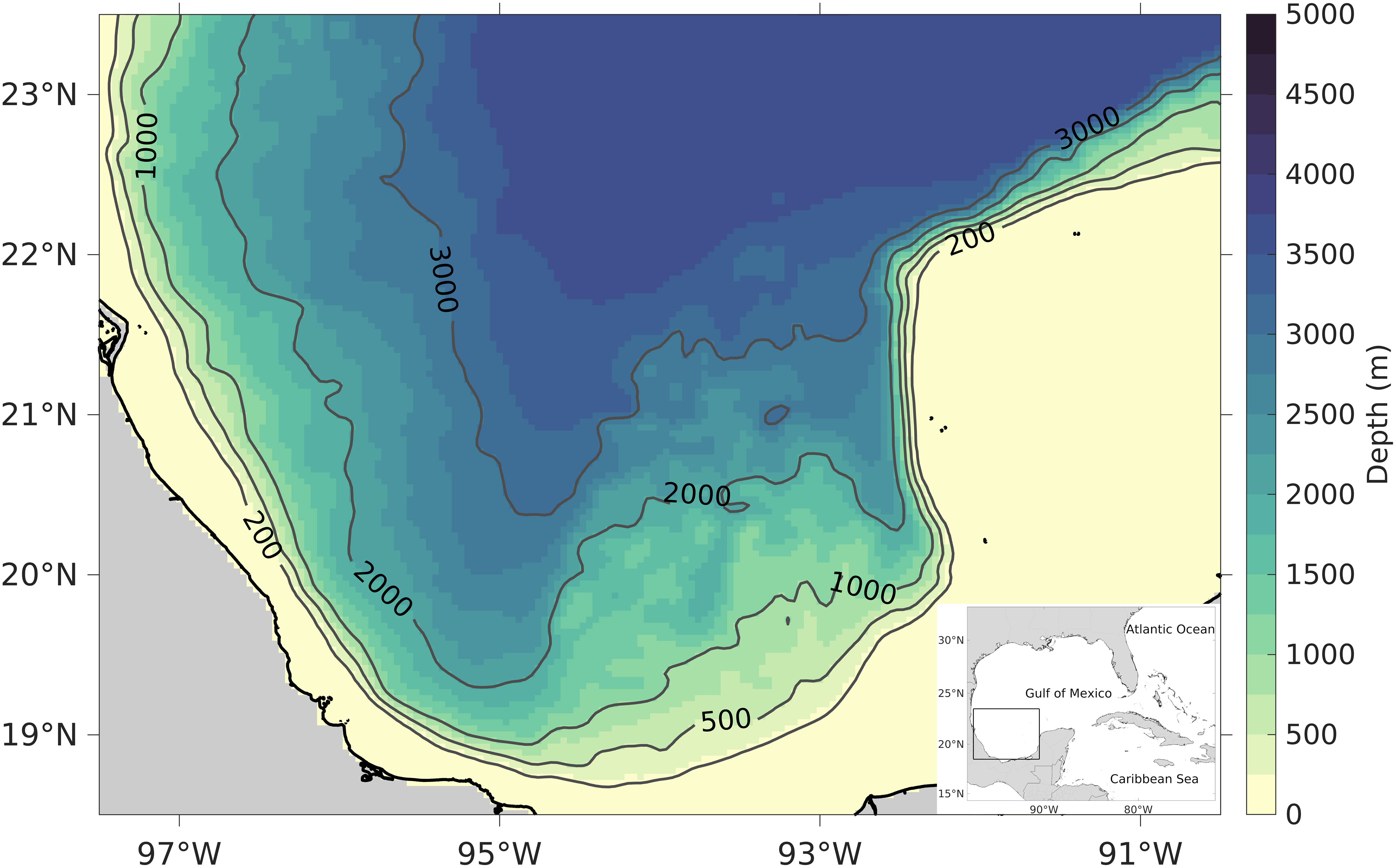
Figure 1 The Gulf of Mexico with a zoom in its southern region. The gray contours represent the 200, 500, 1000, 2000, and 3000 m isobaths.

This study focuses on the southern GoM (Figure 1), a very relevant region in the GoM due to the regular exploration and exploitation of oil and gas developed there (Adams et al., 2004; NOAA, 2008; Yoskowitz et al., 2013) and because it contains some of the most important coral reefs of the GoM (NOAA, 2008; Yoskowitz et al., 2013; Gil-Agudelo et al., 2020). Consequently, studies on mixing processes, dispersion of tracers and pollutants, interchange of tracers between continental shelf waters and the deep ocean, particle dispersion, and ecosystem conservation in the southern GoM are needed (Zavala-Sansón et al., 2017; Gil-Agudelo et al., 2020; Guerrero et al., 2020). The southern GoM circulation is very complex and does not exhibit a clear monthly or seasonal variability pattern; it is composed of many circulation patterns occurring at different spatial scales, lasting from some weeks to a few months (Monreal-Gómez and Salas-de León, 1997; Zavala-Hidalgo et al., 2003; Vázquez de la Cerda et al., 2005; Vukovich, 2007; Dubranna et al., 2011; Pérez-Brunius et al., 2013; Hamilton et al., 2016; Zavala-Sansón et al., 2017; Zavala-Sansón, 2019). The circulation and its associated variability result from the interaction of different ocean mesoscale circulation processes occurring there: a semi-permanent cyclonic circulation referred to as the Campeche Gyre (Monreal-Gómez and Salas-de León, 1997; Vázquez de la Cerda et al., 2005; Pérez-Brunius et al., 2013), a seasonal circulation in the form of an intense alongshore current at the western margin of the basin (Zavala-Hidalgo et al., 2003; Dubranna et al., 2011), and the aperiodic arrival of Loop Current Eddies (Vidal et al., 1992; Vukovich, 2007; Pérez-Brunius et al., 2013; Meza-Padilla et al., 2019).

Observational (Vázquez de la Cerda et al., 2005; Pérez-Brunius et al., 2013) and simplified theoretical and numerical studies (Zavala-Sansón, 2019) have revealed different characteristics of ocean variability in the southern GoM. Vázquez de la Cerda et al. (2005) characterized the mean circulation and variability of the southern GoM using satellite-derived sea surface data, hydrographic data at 425, 800, and 1500 m depth, and drifter and float measurements at 900 m depth. They identified significant circulation patterns in the region, along with their seasonal and non-seasonal variability, temporal variations, and possible associated forcings, emphasizing the Campeche Gyre. Pérez-Brunius et al. (2013) analyzed the surface circulation of the southern GoM using three years of data from surface drifters, current meter moorings (deployed at 500 and 2000 m depth), and satellite altimetry. They observed important effects of Loop Current Eddies on the variability of the Campeche Gyre, whose size and location are delimited by the bathymetry of the region, evincing the relevance of potential vorticity conservation and the equivalent-barotropic model to describe the Gyre dynamics. Zavala-Sansón (2019) used equivalent-barotropic modeling to examine the formation of the Campeche Gyre considering its barotropic vertical structure. He found that the formation of the Gyre is consistent with equivalent-barotropic dynamics and that it is topographically confined according to the shape of the geostrophic contours.

Previous studies have outlined different aspects of the variability, dynamics, and associated forcings of the southern GoM in great detail at the surface and, to a lesser extent, at depths greater than 1000-1200 m. Due to the limited temporal and spatial coverage of data records used in those studies, a comprehensive depiction of deep GoM dynamics still needs to be completed. It remains to be proved if the variability patterns found are persistent, episodic, or representative of GoM dynamics in the long term. Previous research indicated a significant relationship between surface and deep variability in the GoM, with distinctive surface and deep features. Olvera-Prado et al. (2023) studied the coupling between surface and deep layer variability across the entire GoM using thickness data of isopycnic layers from a long-term numerical simulation; they found a strong connection between the layers and associations between the variability modes with recurrent circulation patterns in both layers. However, due to the characteristics of southern GoM dynamics and the implemented methodology, it was not possible to find its regional variability modes. Hence, a thorough description of southern GoM variability throughout the water column has yet to be accomplished.

This work aims to study the extent and characteristics of southern GoM variability throughout the water column, considering the separated variability of a surface and a deep layer and their corresponding coupled variability. Specifically, the following subjects are investigated:

1. The coupling timescales between surface and deep variability.

2. The spatial structure of surface, deep, and coupled variability.

3. The dominant timescales and predictability of surface, deep, and coupled variability.

4. The stochastic origin of southern GoM variability.

In order to achieve these goals, outputs from a 21-year free-running simulation (a simulation without ocean data assimilation) of the GoM hydrodynamics were used. The variability modes were estimated from the layer-thickness field of a surface and a deep isopycnic layer, considering separated and coupled layers analyses. The resulting modes’ spatial structure, dominant timescales, predictability, and stochastic origin were examined.

2 Methods

2.1 Estimation of the variability modes

Oceanic general circulation models are robust and reliable tools for studying the circulation and dynamics of the oceans (Grötzner et al., 1999; Zavala-Hidalgo et al., 2003; Meza-Padilla et al., 2019; Morey et al., 2020; Olvera-Prado et al., 2023). Oceanic general circulation models are robust and reliable tools for studying the circulation and dynamics of the oceans. The characteristics of the numerical models allow for obtaining data continuously. Depending on the physics the models can resolve and the available computing resources to execute them, it is possible to obtain long-term data (several decades) with higher spatial and temporal resolutions than those typical in observations. Specifically, free-running simulations provide a physically consistent description of ocean dynamics that satisfies the primitive equations, allowing a better understanding of ocean dynamics (Morey et al., 2020). This work used the outputs of a 21-year free-running simulation of the GoM hydrodynamics performed with the HYbrid Coordinate Ocean Model (HYCOM), whose characteristics can be reviewed in Olvera-Prado et al. (2023). The simulation covers the period 1992-2012; the horizontal domain covers the region [98°W, 77°W] × [18°N, 32°N], with a 1/25° of horizontal resolution and 27 hybrid vertical layers. The validation of such numerical simulation showed that the simulated GoM hydrodynamics and hydrography are consistent with those obtained using ocean altimetry and in-situ observations (Olvera-Prado et al., 2023).

The most important variability modes were estimated from daily isopycnic layer-thickness anomalies of a surface and a deep layer via the Empirical Orthogonal Functions (EOFs) (Storch and Zwiers, 1999). The surface layer comprises the layers with density values from 17.25 to 26.52, ranging from 0-250 m approximately; the deep layer comprises the isopycnal 27.74 and ranges from 1000-1800 m approximately. The isopycnic layers’ selection is based on the representation of the deep GoM basins as a two-layer system described by Hamilton et al. (2018), in which the 6°C isotherm divides the upper (0− ∼1000 m) and lower (below ∼1000 − 1200 m) layers. In this work, the combined thickness of the surface and deep layers does not cover the total depth of the ocean, so they are not in physical contact; the reason for doing this was to prevent the surface and deep layer fluctuations from mirroring each other, allowing exploring their vertical connection. In addition, the thickness choice of the surface and deep layers made it possible to capture the most energetic component of the variability in each layer, accentuate thickness fluctuations, and reduce the ocean bottom effects on the deep fluctuations.

The variability analysis focuses on the mesoscale, i.e., ocean signals with space scales of 50-500 km and timescales of 10-100 days (CTOH, 2013). Thus, the data were filtered to enhance the mesoscale signal using a low-pass Lanczos filter considering different cutoff periods and a two-dimensional convolution filter considering different space windows. The following study cases were analyzed:

• Case 1: 30-day time filtering and 23 km space filtering.

• Case 2: 30-day time filtering and 69 km space filtering.

• Case 3: 30-day time filtering and 87 km space filtering.

• Case 4: 90-day time filtering and 23 km space filtering.

• Case 5: 90-day time filtering and 69 km space filtering.

However, only the results for Case 2 are shown since it is the most representative of the mesoscale. The trend and annual cycle were removed from the time series of layer-thickness at each grid point, and the correlation matrix was constructed for the surface and deep layers separately. The correlation matrix is the covariance matrix of the standardized anomalies of the data (Wilks, 2019). The variability analyses intend to identify the intercorrelation between the thickness anomalies in the same layer and between the surface and deep layers (characterized by the correlation matrix); they do not intend to identify the strongest variations of thickness anomalies (characterized by the covariance matrix). The following analyses were performed:

1. Separated analysis. It considered an EOF analysis for each layer separately. This work referred to the resulting variability as “separated variability”.

2. Coupled analysis. It considered an EOF analysis for the surface and deep layers data concatenated into a single matrix. This work referred to the resulting variability as “coupled variability”.

In the separated and coupled EOF analyses, the corresponding vector time series $\overrightarrow{X}(\overrightarrow{x},t)$ can be expanded in terms of its spatial patterns, ${\overrightarrow{e}}^{ k}(\overrightarrow{x})$, and their time-varying coefficients, ${\alpha }_k(t)$, also called the principal components (PCs),

$\begin{array}{ll}\overrightarrow{X}(\overrightarrow{x},t)={\displaystyle \sum _k{\alpha }_k(t){\overrightarrow{e}}^{ k}(\overrightarrow{x}),}& (1)\end{array}$

where $\overrightarrow{x}$ denotes the spatial coordinates, $t$ denotes time, and $k$ runs over the dimension of $\overrightarrow{X}(\overrightarrow{x},t)$. Since ${\overrightarrow{e}}^{ k}$ is orthogonal to each other, the regions well explained by each spatial pattern are different. A common approach to identify the regions well explained by a particular set of EOFs $\left\{{\overrightarrow{e}}^{ m}\right\}$ is to compute its proportion of explained variance (PEV),

$\begin{array}{ll}\text{PEV}(\overrightarrow{x})=1-\frac{var(\overrightarrow{X}-{\displaystyle {\sum }_m{\alpha }_m{\overrightarrow{e}}^{ m}})}{var(\overrightarrow{X})},& (2)\end{array}$

where var denotes variance. Similar to ${\overrightarrow{e}}^{ k}$, PEV can also be displayed as a map. Since the PEV represents the proportion of the total variance of the data explained by a particular set of EOFs, the spatial patterns are significant only in the regions with large PEV; these regions are statistically meaningful and were used to describe the spatial variability of the southern GoM. Generally, the regions with large EOF amplitude coincide with those with large PEV.

2.2 Predictability timescale

The predictability timescales of southern GoM variability were estimated by analyzing the characteristic properties of the PCs of each EOF analysis using time series analysis techniques (Storch and Zwiers, 1999; Box et al., 2015; Brooks, 2019). It was supposed that the predictability skill of southern GoM variability depends on the persistence of the PCs. The PCs can be grouped into processes with long or short memory depending on the persistence of their current values. In long-memory processes, the current value tends to persist during long periods, resulting in processes with long-term persistence; in short-memory processes, the values persist during shorter periods (Storch and Zwiers, 1999; Brooks, 2019). Thus, the skillfulness of the persistence forecasts is greater for long-memory processes than for short-memory processes and is highly determined by their corresponding auto-correlation functions (Storch and Zwiers, 1999).

The predictability timescale for each mode of southern GoM variability was estimated using a measure of the decorrelation time τ of the corresponding PC for each EOF analysis,

$\begin{array}{ll}\tau =1+2{\displaystyle \sum _{k=1}^{\infty }{\rho }^2(k),}& (3)\end{array}$

where ρ (k) is the auto-correlation function of the corresponding PC at discrete lag k. This work supposes that autoregressive processes of order p, or AR(p) processes, can describe the PCs. AR(p) processes are an important class of time series models (Brooks, 2019), widely used in climate research because they represent discretized versions of ordinary differential equations (Storch and Zwiers, 1999) and because they are helpful in modeling and predicting a variable of interest using only its own and past values, without the necessity of specifying a theoretical model of its behavior (Brooks, 2019). With this approach, an AR(p) process was fitted to each PC following Box et al. (2015), the theoretical auto-correlation functions of the fitted AR processes were obtained by solving the Yule-Walker equations following Storch and Zwiers (1999), and their predictability timescales were estimated using Equation (3).

Trenberth (1985) proposed the decorrelation time given by Equation (3) as an indicator of the persistence timescale of the corresponding time series and its associated processes. DelSole (2001) showed that Equation (3) arises naturally in statistical sampling theory and provides an accurate predictability estimate for oscillatory auto-correlation functions. Buckley et al. (2019) used this definition of the decorrelation time to estimate the predictability timescales for sea surface temperature and upper-ocean heat content in the North Atlantic. Because τ is based solely on the local auto-correlation function, it can be interpreted as a lower bound on the predictability timescale since skillful predictions, at least as long as τ, can be made using linear regression, where the inclusion of additional predictors can extend the predictability timescale (Buckley et al., 2019).

2.3 Stochastic origin of variability

The stochastic origin of variability is based on the stochastic null hypothesis of climate variability proposed by Hasselmann (1976), which says that the long-term (or low-frequency) variability of a system can be understood as the integrated response of it driven by high-frequency fluctuations. The stochastic climate model of Hasselmann can be derived via a statistical dynamical model in terms of a fast (e.g., atmosphere) and a slow (e.g., ocean) component of the climate system (Storch and Zwiers, 1999), resulting in that, to first order, the long-term variability can be explained by an AR(1) process.

The AR(1) process is commonly taken as the null hypothesis to explain long-term variability (Grötzner et al., 1999; Storch and Zwiers, 1999; Dommenget and Latif, 2002). Several hypothesis tests have been developed to investigate the adequacy of this null hypothesis in describing long-term variability. The following two hypothesis tests were used to investigate the stochastic origin of southern GoM variability, considering the PCs of each EOF analysis (subsection 3.4). This work fitted an AR(1) process to each PC following Box et al. (2015). The fitted AR(1) process represents the null AR(1) process, and its spectrum represents the corresponding null AR(1) spectrum, that is, the reference spectrum against which the PC spectrum was compared and used to perform the hypothesis tests.

● Wilks (2019) describes a hypothesis test whose null hypothesis states that the arising of the process of interest from a given null process cannot be rejected at a specified level if its largest spectral coefficient does not rise above the corresponding rejection limit curve of the null spectrum. This work examined the statistical significance of the largest spectral peak in the sample spectrum of each PC considering rejection limits at the 0.01 level in each null AR(1) spectrum.

● Dommenget and Latif (2002) developed a statistical test to test if the power spectral density (PSD) increase of a process of interest is consistent with a fitted AR process. It assumes that the sample spectral coefficients of the process of interest are random fluctuations around the spectral coefficients of the null spectrum based on a test quantity T defined as

$\begin{array}{ll}T=\frac{1}{\text{ln}({\sigma }_{spec})}\sqrt{{\displaystyle \sum _{i=2}^N\frac{[\text{log}(s_i)-\text{log}(t_i){]}^2}{N-1}}},& (4)\end{array}$

● where $s_i$ are the spectral coefficients of a PC, $t_i$ are the spectral coefficients of the corresponding null AR(1) spectrum, $N$ is the number of spectral coefficients, and ${\sigma }_{spec}$ is the standard deviation of $s_i$. The confidence levels relative to the statistical distribution of the test quantity are derived using Monte Carlo statistics; in this work, such levels were derived from $100000$ realizations of null AR(1) processes. The hypothesis test was implemented to the sample spectra of each PC up to the frequency of $12$ cpy ($30$ days) to avoid possible discrepancies by the application of the low-pass Lanczos filter to the PC series.

3 Results

3.1 Surface-deep coupling timescales of southern GoM variability

This subsection analyzes the correlation between the variability of the surface and deep layers for different time lags between them. The objective is to investigate the timescales in which surface and deep variability are strongly connected, for which a coupled EOF analysis was performed considering lags from 1000 to −1000 days of the surface layer relative to the deep layer. For example, a lag of 250 days means that the surface layer is shifted forward in time 250 days relative to the deep layer. For the lags of ±1000 days, the resulting time series corresponds to a reduction of 13% in the total length of the analyzed data.

Figure 2 shows the contained variance in the first four modes considering different time lags of the surface layer relative to the deep layer (the results are very similar for the other study cases mentioned in subsection 2.1); the figure only shows the results when the set of modes is not degenerate according to the rule of thumb of North et al. (1982). The contained variance is taken as a measure of the coupling’s strength between surface and deep variability for a given lag: a high variance corresponds to strong coupling, whereas a small variance corresponds to weak coupling. The percentage of the total variance contained in the first four modes varies little (from 39-44%) for lags from 1000 to -1000 days of the surface layer relative to the deep layer; the southern GoM variability is very complex, resulting in a non-evident coupling between its surface and deep variability. The most intense coupling for a particular state of surface variability at a given time is found with the concurrent and quasi-concurrent states of deep variability. The coupling between surface variability and deep variability is slightly higher for previous states of deep variability than for subsequent states of it, which could suggest that deep variability precedes surface variability and that the deep layer is more likely to influence the subsequent evolution of the surface layer than the other way around. Nonetheless, since the suggested direction of information transmission between the layers was obtained through purely statistical analysis, additional specific analyses are required to establish causality relationships between the deep and surface layers.

FIGURE 2

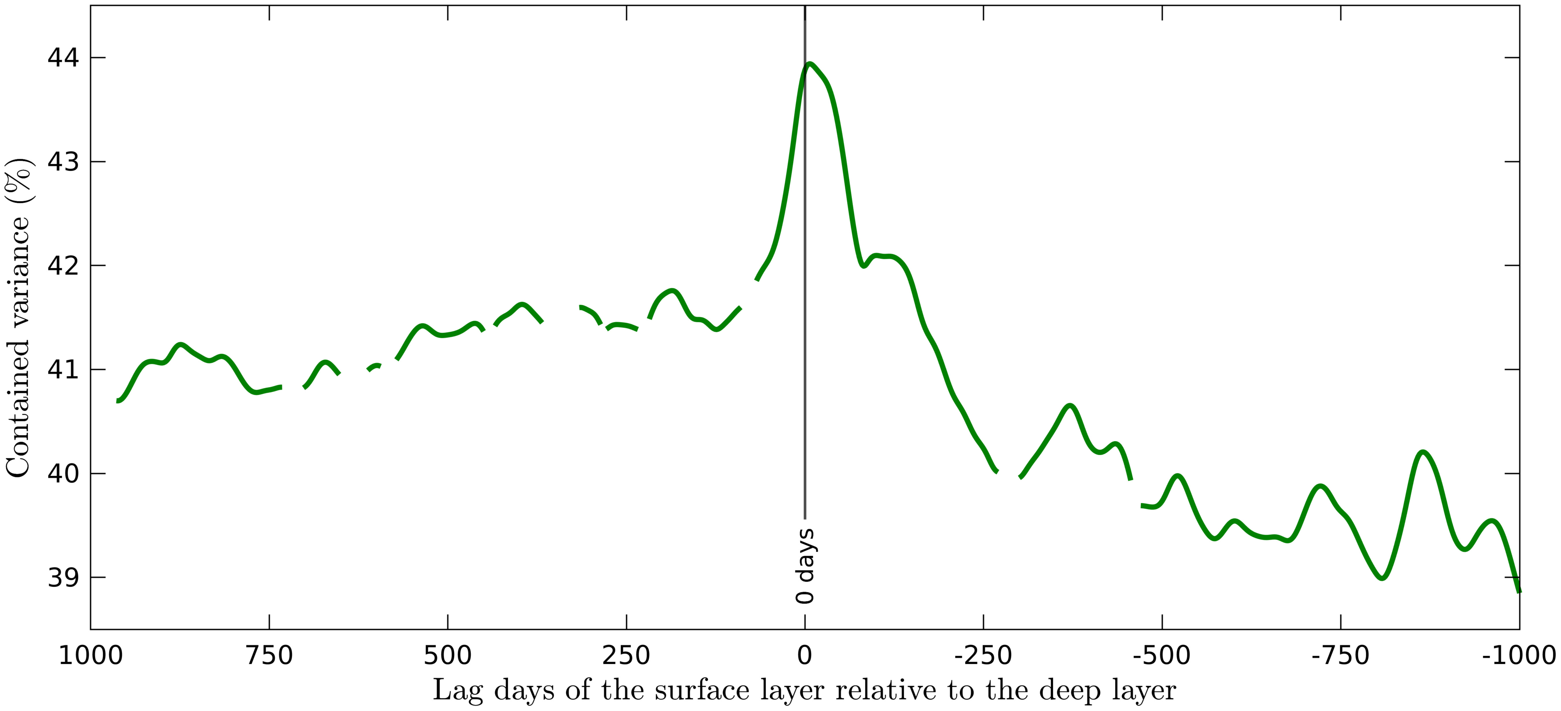
Figure 2 Contained variance in the first four modes for the coupled EOF analysis considering different time lags of the surface layer relative to the deep layer. Only the cases for which the modes are not degenerate, according to the rule of thumb of North et al. (1982), are shown.

In order to perform an analysis of coupled variability in the southern GoM resulting in coupled modes with the highest possible contained variance, a coupled EOF analysis with a zero-day lag between the surface and deep layers was considered. Given the chosen zero-day lag, the coupled analysis describes concurrent spatial variability between the surface and deep layers; it identifies surface and deep regions spatially connected and the characteristics of that connection.

The distribution of contained variance in each mode for the separated and coupled EOF analyses (Table 1) indicates that southern GoM variability is a complex process. The total variance is distributed in many modes, and no single mode contains a considerable portion of it. For the separated analyses, the first mode contains a quarter of the total variance; the contained variance in the first mode is slightly smaller for the coupled analysis. The decrease in contained variance for the higher-order modes is smaller for the surface layer, then for the deep layer, and ultimately for the coupled layers; such behavior can be transferred to the ability to define the corresponding variability. Because the contained variance in the first four modes is significant for the separated and coupled EOF analyses, it is assumed that these modes describe the predominant southern GoM variability well and that the study of it can be adequately addressed via EOFs decomposition.

TABLE 1

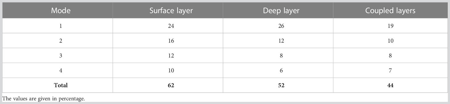
Table 1 Distribution of contained variance in the first four modes for the separated and coupled EOF analyses.

3.2 Spatial patterns of southern GoM variability

What characteristics would the spatial patterns obtained from the isopycnic layer-thickness field have? In the surface layer, the isopycnic layer-thickness contours are a good proxy of circulation since they closely follow the flow streamlines; thus, the EOFs reflect where the main circulation variability occurs. In the deep layer, the isopycnic layer-thickness contours are not a good circulation proxy (Cushman-Roisin et al., 1990; Olvera-Prado et al., 2023). Nonetheless, since the isopycnic layer-thickness structure throughout the water column responds to pressure gradients, layer-thickness variability (and thus the associated EOFs) is expected to reflect regions with high circulation variability in each layer. Moreover, due to the weak deep GoM stratification, a bathymetry-influenced deep variability, strongly governed by the conservation of potential vorticity, is also expected. Accordingly, a description of surface and deep circulation variability of the southern GoM is first presented (Figure 3) and then referred to when describing the EOFs (Figure 4).

FIGURE 3

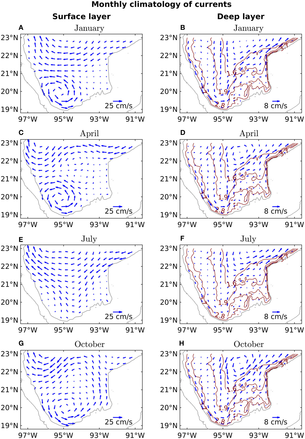
Figure 3 Monthly climatology of vertically averaged currents in the southern Gulf of Mexico in a surface layer (0-250 m) and a deep layer (1000-1500 m) derived from the HYCOM simulation. The brown lines in the deep layer maps represent the planetary potential vorticity contours in (s·m)^-1.

FIGURE 4

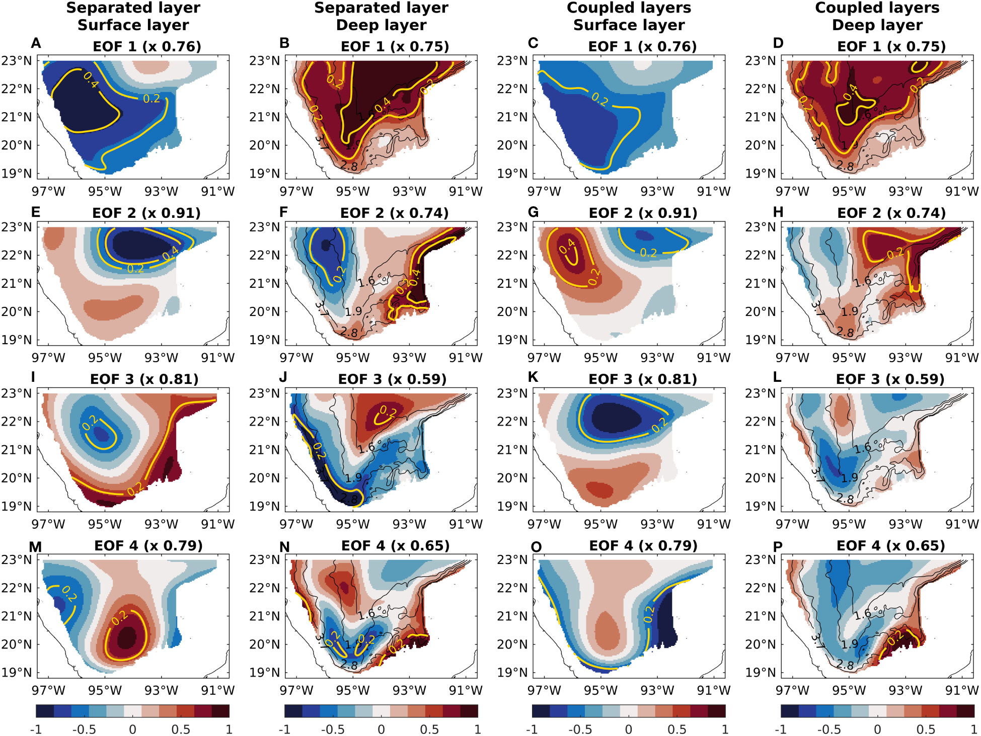
Figure 4 First four EOFs of the surface and deep layers for the separated and coupled EOF analyses. The EOF amplitude is shown in color scale, and yellow contours represent the proportion of explained variance of each EOF. The black lines in the deep layer maps represent the planetary potential vorticity contours in (s·m)^-1.

Figure 3 shows a monthly climatology of vertically averaged currents in a surface layer (0-250 m) and a deep layer (1000-1500 m) for the 21 years of simulation. The brown lines in the deep layer maps represent planetary potential vorticity ($f/H$) contours, where $f$ is the local Coriolis parameter, and $H$ is the bottom depth. In the surface layer, the currents’ speed is approximately three times greater than in the deep layer, with significant changes in the circulation patterns throughout the year, in contrast to the more persistent deep circulation. The changes in surface circulation patterns (panels of the first column in Figure 3) can be described as follows:

1. In the region north of ${20.5}^{\circ }\text{N}$ and west of ${93.5}^{\circ }\text{W}$, an intense and well-defined anticyclonic circulation occurs during winter and summer. During fall, the circulation in the region $({95.0}^{°}\text{W},{93.5}^{°}\text{W})\times ({20.5}^{°}\text{N},{23.0}^{°}\text{N})$ is cyclonic, with a weak intensity in its interior and southern branch. During spring, the region $({95.0}^{\circ }\text{W},{93.5}^{\circ }\text{W})\times ({20.5}^{\circ }\text{N},{23.0}^{°}\text{N})$ is occupied by a dipole, with a cyclone and an anticyclone oriented from north to south; the circulation is weak in the interior and the eastern branch of the dipole.

2. The circulation in the region east of 93.5°W and north of ${22.0}^{\circ }\text{N}$ is intense and northeasterly during winter and summer, weak and anticyclonic during fall, and intense and easterly during spring. The circulation changes in the northern region are probably associated with the arrival or generation of cyclonic and anticyclonic mesoscale features (Zavala-Sansón et al., 2017; Guerrero et al., 2020).

3. The circulation in the region $({93.5}^{\circ }\text{W},{92.5}^{\circ }\text{W})\times ({20.0}^{\circ }\text{N},{22.0}^{\circ }\text{N})$ is feeble and northerly during most of the year, but during fall, it is intense and southerly.

4. To the southeast of the basin, west of $94.0°\text{W}$ and south of ${21.0}^{\circ }\text{N}$, there is a cyclonic circulation, the Campeche Gyre (Vázquez de la Cerda et al., 2005; Pérez-Brunius et al., 2013; Zavala-Sansón, 2019). During winter and spring, the Gyre is intense and located to the northwest; it weakens until its dissipation in summer; in fall, the Gyre re-forms in a southeast location.

The circulation patterns in the deep layer (panels of the second column in Figure 3) have small variations throughout the year, reaching their minimum intensity during summer. The circulation is aligned with the planetary potential vorticity contours with a cyclonic rotation sense: west of ${95.0}^{\circ }\text{W}$, the currents go from north to south, and east of ${95.0}^{\circ }\text{W}$, the currents go from south to north. The circulation in the southeast region, where the bathymetry is abrupt, is weak, with few changes throughout the year. The changes in deep circulation patterns can be described as follows:

1. In the region north of ${21.0}^{\circ }\text{N}$ and east of ${95.0}^{\circ }\text{W}$, roughly limited by the 1.6 (s·m)⁻¹ planetary potential vorticity contour, there is an intense and well-defined cyclonic circulation throughout the year. This circulation is shifted to the south during spring and fall, whereas it is shifted to the northeast during winter and summer.

2. In the region between $({96.5}^{\circ }\text{W},{95.0}^{\circ }\text{W})$ and north of ${20.0}^{\circ }\text{N}$, there is a year-round northerly circulation, with a weak western branch and an intense eastern branch. The western branch circulation strengthens during spring and weakens during winter, summer, and fall; the eastern branch strengthens during winter and fall and weakens during spring and summer.

3. The circulation intensity in the eastern boundary north of ${20.0}^{\circ }\text{N}$ and the western boundary varies throughout the year. It strengthens during winter and fall and weakens during spring and summer.

4. The intensity of the cyclonic circulation along ${19.5}^{\circ }\text{N}$ and between $({95.5}^{\circ }\text{W},{94.5}^{\circ }\text{W})$ remains intense most of the year except during summer.

Figure 4 shows the first four EOFs of the surface and deep layers for the separated and coupled EOF analyses. The EOF amplitude is shown in color scale, and yellow contours represent the PEV of each EOF. Due to the thickness data processing (subsection 2.1), the EOFs are assumed to represent the mesoscale variability in each layer adequately.

First, the separated variability modes are described (panels of the first and second columns in Figure 4). The first four EOFs in both layers are well-defined and recognizable, and together they occupy the entire basin. As expected, the EOFs identify regions with high circulation variability in both layers (Figure 3); they rank variability modes based on their contained variance but are not expected to identify individual dynamical modes (Storch and Zwiers, 1999; Monahan et al., 2009). In the deep layer, the bathymetry influences the variability; layer-thickness variations align with the planetary potential vorticity contours and intensify along bottom slopes. The spatial variability modes are described below:

1. The principal variability in the surface layer (Figure 4A), mainly located in the northwest, is associated with variations in the anticyclonic circulation north of ${20.5}^{\circ }\text{N}$ and west of ${94.5}^{\circ }\text{W}$ (panels of the first column in Figure 3). The principal variability in the deep layer (Figure 4B), covering a wide area north of ${20.0}^{\circ }\text{N}$, is associated with latitudinal shifts of the long-scale cyclonic circulation in that region (panels of the second column in Figure 3).

2. The spatial pattern of the second mode in the surface layer (Figure 4E) shows high variability in the region east of ${95.0}^{\circ }\text{W}$ and north of ${21.5}^{\circ }\text{N}$, associated with changes in the intensity and direction of the circulation in the northern region (panels of the first column in Figure 3). The spatial pattern in the deep layer (Figure 4F) shows high variability along ${96.0}^{\circ }\text{W}$ and north of ${21}^{°}\text{N}$ and along the eastern basin boundary, mainly associated with variations in the circulation intensity in those regions (panels of the second column in Figure 3).

3. The third mode in the surface layer (Figure 4I) reflects variability along the eastern and southern boundaries, which is associated with changes in the intensity and direction of the circulation in that region (panels of the first column in Figure 3). In the deep layer (Figure 4J), the variability is located along the western boundary, which is associated with variations in circulation intensity in that region; and in a spot centered at $({94.0}^{\circ }\text{W},{22.0}^{\circ }\text{N})$, associated with latitudinal shifts of the cyclonic circulation in that region (panels of the second column in Figure 3).

4. The spatial pattern of the fourth mode (Figure 4M) shows high surface variability in a spot centered at $({94.0}^{°}\text{W},{20.0}^{°}\text{N})$, which is associated with changes in the intensity and direction of the circulation in that region (panels of the first column in Figure 3). The deep variability (Figure 4N) is represented by a lobe form centered at $({95.0}^{°}\text{W},{19.5}^{°}\text{N})$, which is associated with intensity variations of the cyclonic circulation in that region (panels of the second column in Figure 3).

The spatial patterns of coupled variability (panels of the third and fourth columns in Figure 4) differ from those of separated variability (panels of the first and second columns in Figure 4), which could indicate a significant connection between the surface and deep layers. By comparing the spatial structure and time evolution of coupled and separated variability, it is possible to obtain insights into the dynamics of southern GoM variability throughout the water column. The first four EOFs in the surface layer (panels of the third column in Figure 4) are well-defined, recognizable, and significant (they have spatial regions with appreciable PEV). However, only the first two modes in the deep layer (panels ofthe fourth column in Figure 4) are significant; the third and fourth modes lack spatial regions with appreciable PEV, indicating that higher-order surface variability has no connection with deep variability. Results also show no vertical correspondence between surface and deep layer-thickness variations; the fluctuations of deep isopycnals do not mirror those of surface isopycnals. The spatial variability modes are described below:

1. The principal coupled variability in the surface layer (Figure 4C), described by a confined southwestern region where the Campeche Gyre occurs, is associated with the strengthening and dissipation of the Campeche Gyre and with its latitudinal and longitudinal shifts (panels of the first column in Figure 3). In the deep layer (Figure 4D), the variability is mainly described by a small region centered at $({95.0}^{\circ }\text{W},{21.5}^{\circ }\text{N})$, associated with the southernmost intrusion of the cyclonic circulation in that region; and by a wide region north of ${20.0}^{\circ }\text{N}$, associated with long-scale variations of the cyclonic circulation in the region east of ${95.0}^{\circ }\text{W}$ and north of ${20.0}^{\circ }\text{N}$ (panels of the second column in Figure 3). The deep pattern is very similar to that of the first mode of the separated deep layer.

2. The spatial pattern of the second mode in the surface layer (Figure 4G), described by a zonal dipole north of ${21.0}^{\circ }\text{N}$, is associated with variations in the circulation in the northern region (panels of the first column in Figure 3). In the deep layer (Figure 4H), the spatial pattern shows high variability in the northeast, which is associated with variations in the circulation intensity along the eastern boundary and with latitudinal shifts of the cyclonic circulation east of ${95.0}^{\circ }\text{W}$ and north of ${21.0}^{\circ }\text{N}$ (panels of the second column in Figure 3).

3. The third coupled mode in the surface layer (Figure 4K) is very similar to the second separated mode in the surface layer (Figure 4E). The fourth coupled mode in the surface layer (Figure 4O) shows high variability in the southeastern region, associated with variations in the circulation intensity in that region. These surface modes have no associated deep modes (Figures 4L, P) since these are not recognizable due to their marginal PEV.

3.3 Predictability of southern GoM variability and associations between separated and coupled variability

The predictability timescales of southern GoM variability were estimated by considering the decorrelation time (subsection 3.2) of each PC for the separated and coupled EOF analyses. The fitting of an AR model to each PC resulted in an AR(5) for each. Figure 5 shows the predictability timescales for the first four variability modes of the surface, deep, and coupled layers; the predictability timescales of the PCs are representative of the characteristic timescales of the corresponding spatial variability. The shortest predictability timescales are for the surface layer, with values from 1.4 to 10.6 months, which reminds the dominant timescales of mesoscale variability in the southern GoM (Vázquez de la Cerda et al., 2005; Pérez-Brunius et al., 2013; Zavala-Sansón et al., 2017). The deep layer has the longest predictability timescales, with almost three times the scales of the surface layer, from 3.0 to 30.5 months. Deep variability is more persistent and changes in longer timescales than surface variability, in agreement with the temporal change of surface and deep currents (monthly climatology of currents shown in Figure 3).

FIGURE 5

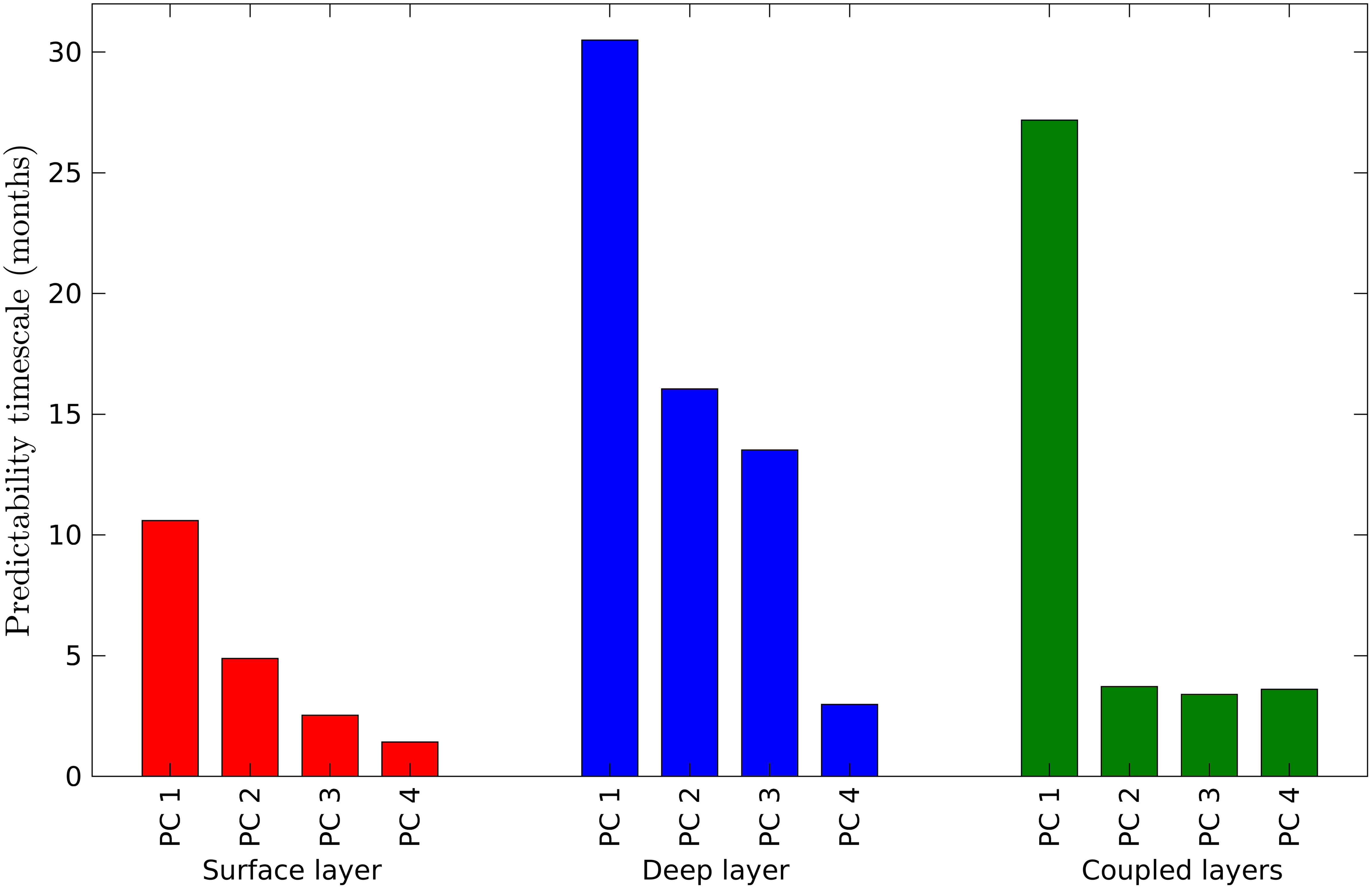
Figure 5 Predictability timescales of the first four principal components (PCs) for the surface, deep, and coupled layers.

The predictability timescales of the coupled layers depend on the coupling’s strength of the surface and deep layers. The predictability timescales for the coupled layers lie between those for the surface and deep layers but closer to those of the deep layer, with values from 3.4 to 27.2 months (Figure 5). Such behavior indicates that the memory of the coupled system resides in the deep layer but only for the first variability mode. By coupling a system composed of a fast (the surface ocean layer in this study) and a slow (the deep ocean layer in this study) component, the predictability of the fast component can be extended by coupling it with the slow component (Hasselmann, 1976; Grötzner et al., 1999; Dommenget and Latif, 2002). Nevertheless, the intensity of the coupled system’s high-frequency internal noise could weaken the coupling’s strength and drastically reduce its predictability timescale. The predictability timescales for the coupled system have the following behavior (Figure 5):

• First mode. The long predictability timescale for this mode suggests an intense surface-deep coupling, in which both layers evolve conjointly with a predictability timescale of 27.2 months. The predictability timescale in the surface layer was substantially extended by a factor of 2.6 compared with that of the separated surface layer, resulting in a very similar timescale to that of the separated deep layer. The predictability timescale in the deep layer is very similar to that of the separated deeplayer (30.5 months).

• Higher-order modes. The surface-deep coupling is not strong enough to extend the predictability timescales in the surface layer with respect to those obtained in the separated analysis. Such weak surface-deep coupling resulted in predictability timescales in the deep layer similar to those of the separated surface layer.

The previous analysis indicated a connection between the surface and deep layers in the southern GoM, in which the coupled variability (variability throughout the water column) is more similar to the deep variability, at least for the principal variability mode. In order to explore further the connection of coupled variability with surface and deep variability, the similarity between each coupled PC and each surface and deep PC was examined considering two standard similarity measures, the root mean square similarity and Pearson’s correlation, where 1 indicates the maximum similarity (Cassisi et al., 2012). Figure 6 shows the similarity analysis, which helps reveal the coupling’s strength between coupled and separated variability. The first three coupled PCs have a clear and dominant association with a separated PC. The coupled PC 1 is mainly associated with the deep PC 1. The coupled PC 2 is highly associated with the deep PC 2. The coupled PC 3 is mainly associated with the surface PC 2; from the previous analysis of spatial variability, it is an expected result since the third coupled mode in the surface layer (Figure 4K) is practically the same as the second separated mode in the surface layer (Figure 4E).

FIGURE 6

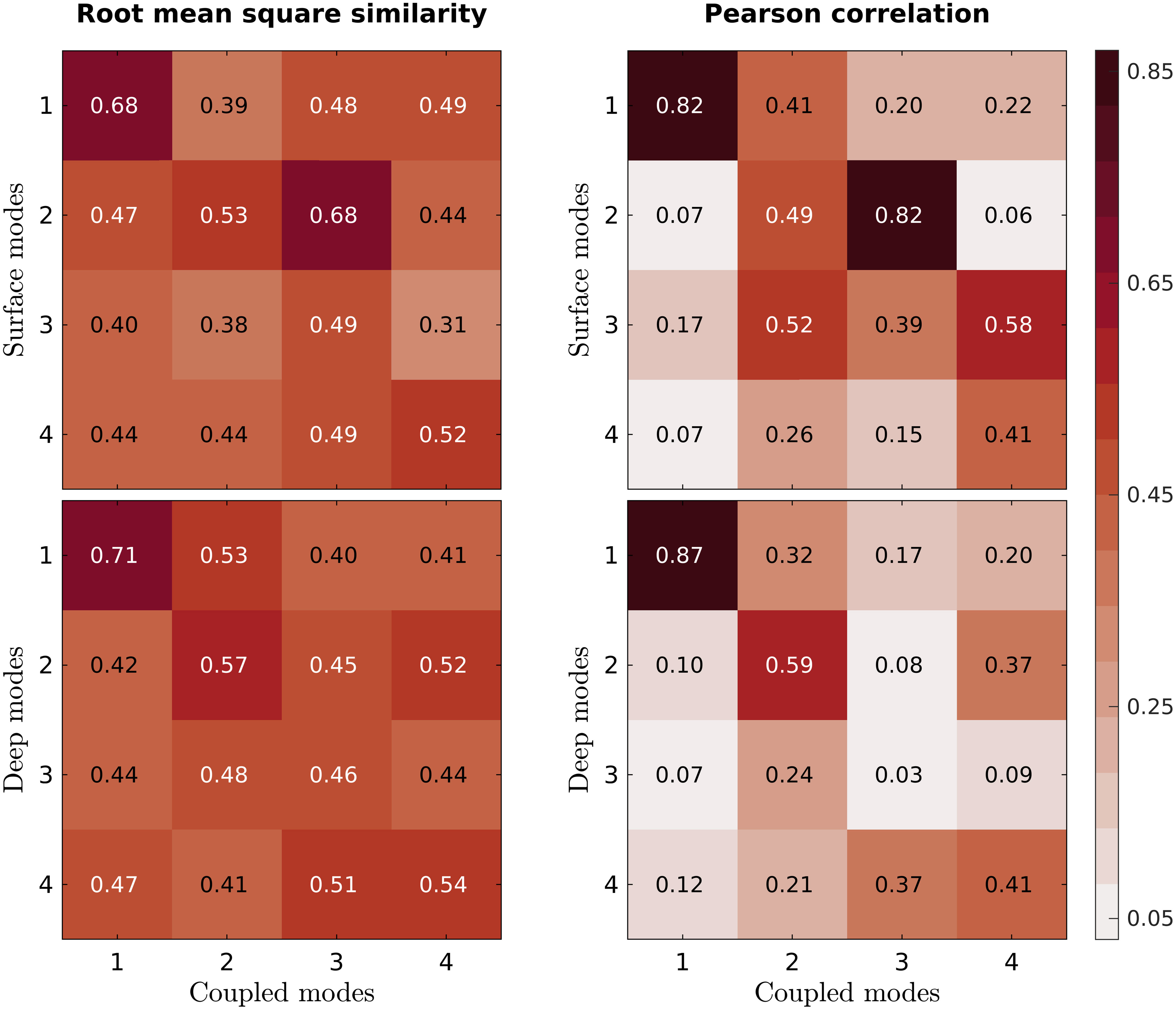
Figure 6 Similarity measures for each combination of principal components (PCs) considering the separated and coupled EOF analyses of southern GoM variability. For Pearson’s correlation, its absolute value is shown.

The connection between coupled and separated variability is also appreciable in the time domain. Figure 7 shows the time series of the first three PCs of coupled layers with their corresponding associated PCs of separated layers. Their temporal nature is described below.

FIGURE 7

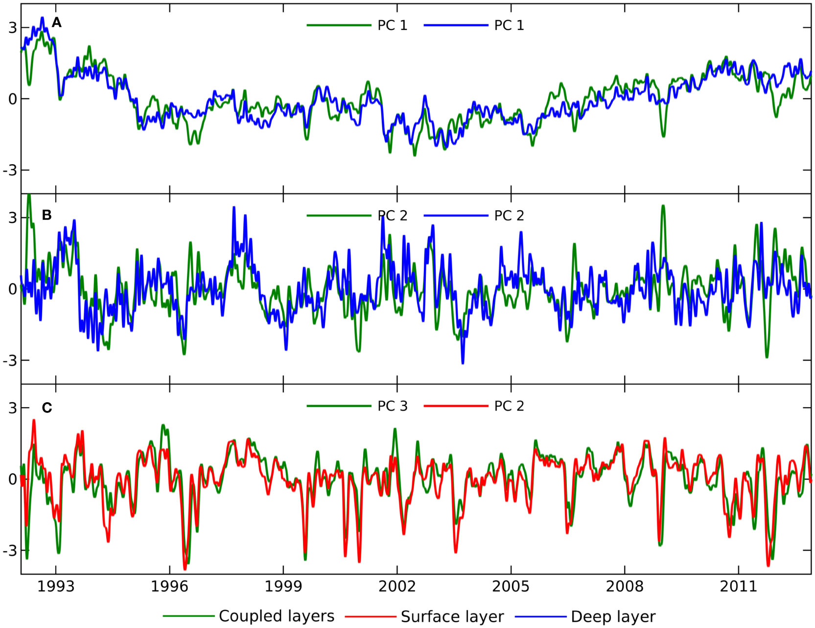
Figure 7 Time series of the first three principal components (PCs) of coupled layers with their corresponding associated PCs of separated layers. (A) Coupled PC 1 and deep PC 1. (B) Coupled PC 2 and deep PC 2. (C) Coupled PC 3 and surface PC 2.

• The PCs for the first variability mode of the coupled and deep layers (Figure 7A) are very similar, as are their corresponding spatial patterns (Figures 4D, B). The PCs evolve in long timescales, with negative or positive values maintained for extended periods, although their wiggles do not always coincide; they are very time persistent and have the longest predictability timescale among all the variability modes (Figure 5).

• The PC for the second coupled variability mode evolves with more accentuated short-term variations and has a high similitude with the deep PC 2 (Figure 7B). Such short-term variations in both PCs resulted in a low time persistence and short predictability timescales (Figure 5) of their associated spatial patterns (Figures 4F, G, H).

• The PC for the third coupled mode is practically the same as for the second surface mode (Figure 7C); their corresponding spatial patterns (Figures 4K, E) are also practically the same. Due to the evolution with high-frequency variations of these modes, their time persistence is low, and their predictability timescales are short (Figure 5).

There is a similarity between the variability modes obtained in the coupled and separated layers analyses. Nevertheless, some coupled modes differ from all those obtained in the separated layers analyses, suggesting that these result from the surface-deep coupling. Examples of this coupling are the spatial pattern of the first mode in the surface layer (Figure 4C) and the patterns of the second mode in both layers (Figures 4G, H).

3.4 Stochastic origin of southern GoM variability

As a preamble to analyze the stochastic origin of southern GoM variability, the distinctive timescales of surface, deep, and coupled variability of the southern GoM were revisited using the spectra of their PCs (Figure 8). Figure 8 shows the sample spectra (cyan lines) and multitaper spectra (blue lines) of the first four PCs for the separated and coupled EOF analyses, with their corresponding null AR(1) spectra (solid red lines) and rejection limits at the 0.01 level (dashed red lines). The multitaper method consistently estimates a process’s true PSD by averaging a set of modified periodograms obtained using several tapers as windowing functions, reducing spectral leakage (Thomson, 1982). In terms of the PSD of a process, the longer the memory of the process, the higher its values for frequencies approaching zero. The principal variability mode for the separated and coupled layers (Figures 8A-C) varies over long timescales. The PSD of the PC increases with decreasing frequency (a typical red noise process), leading to the associated spatial patterns (Figures 4A-D) being long-term persistent. The long-term persistence of the principal mode is stronger in the deep layer (Figure 8B) than in the surface layer (Figure 8A), showing the well-known fact that the deep layer evolves in longer timescales than the surface layer. The PSD increase of the principal mode of the coupled layers (Figure 8C) is very similar to that of the deep layer (Figure 8B), indicating that the timescales of coupled variability are similar to those of deep variability.

FIGURE 8

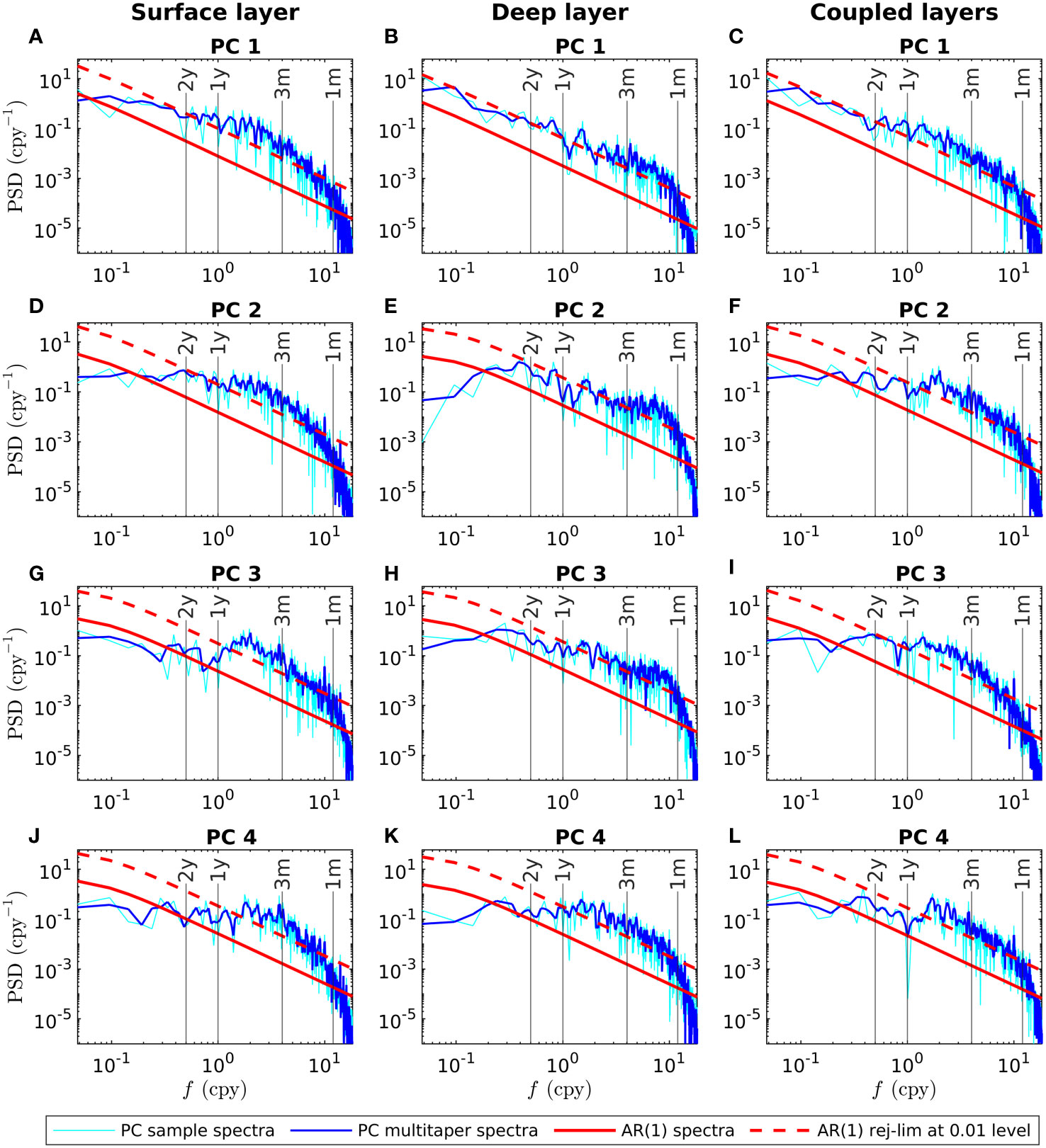
Figure 8 Sample spectra (cyan lines) and multitaper spectra (blue lines) of the first four principal components (PCs) for the separated and coupled EOF analyses. The spectra of the AR (1) models fitted to each PC (the null AR(1) spectra) are plotted using solid red lines, with their corresponding rejection limits at the 0.01 level plotted using dashed red lines. PSD stands for power spectral density.

In agreement with the predictability timescales analysis (Figure 5), the higher-order variability is not long-term persistent; the PSD of the associated PCs does not consistently increase with decreasing frequency (Figures 8D-L). In the surface layer (Figures 8D, G, J), a significant portion of the PSD is concentrated in the three-month to one-year period band, with a small decrease for periods longer than one year. The PSD increase in the deep layer (Figures 8E, H, K) has a small bump in the one-month to three-month period band and a pronounced decrease for periods longer than one year. For the coupled layers (Figures 8F, I, L), a large portion of the PSD is concentrated in the three-month to one-year period band, with a small decrease for periods longer than one year. In summary, higher-order coupled modes vary on similar timescales to higher-order surface modes but without an associated correspondence between the modes of the same order.

When considering coupled variability of the southern GoM, there is a separation between its principal and higher-order modes (Figures 2 and 4−8). Its principal variability (timescales and long-term persistence) is mainly associated with its deep dynamics; the deep layer strongly determines the principal variability throughout the water column. Its higher-order variability has surface and deep dynamics characteristics, with no clear association with one of them.

Now it is the turn to explore the stochastic origin of the long-term variability of the southern GoM, considering the two hypothesis tests described in subsection 2.3. First, the analysis was performed considering the hypothesis test described by Wilks (2019). For this, the spectra of the PCs and the spectra of the AR(1) models fitted to each of them (the null AR(1) spectra of the PCs) shown in Figure 8 were used. All the PC spectra do not rise above their AR(1) rejection limits at frequencies lower than 0.5 cpy (periods longer than two years), but they do rise above them at frequencies higher than 0.5 cpy (periods shorter than two years). Thus, the simplest stochastic model adequately describes only the long-term variability of the surface, deep, and coupled layers in the southern GoM. The high thermal inertia of the isopycnal layers acts as a memory, integrating short-term random variations and carrying energy to the long term in the manner described by Hasselmann (1976), producing a reddened spectrum consistent with an AR(1) process at frequencies lower than 0.5 cpy. On the other hand, the PC spectra deviate from their corresponding null AR(1) spectra at frequencies higher than 0.5 cpy. Southern GoM variability in timescales from some weeks to a couple of years is strongly affected by the episodic occurrence of different mesoscale circulation processes (Vázquez de la Cerda et al., 2005; Pérez-Brunius et al., 2013; Zavala-Sansón et al., 2017; Guerrero et al., 2020), which could explain the PC spectra deviations described above.

The results of the hypothesis test proposed by Dommenget and Latif (2002) are shown in Table 2, considering null AR(1) and AR(2) spectra and a rejection limit at the 0.05 level. The PSD increase of each first PC is consistent with an AR(1) process, indicating that their source of long-term variability can be associated only with short-term random variations. The principal variability mode of the surface, deep, and coupled layers agrees with the stochastic null hypothesis of Hasselmann (1976); they can be described using a linear dynamics approach in terms of a fast and a slow component, with the involved dynamical processes grouped in one of those components (Storch and Zwiers, 1999). The random origin of the principal variability of the southern GoM does not mean that it is not predictable at all; only a completely random process such as AR(0) is not predictable at all. The performed fitting of higher-order AR models to the PCs to estimate their predictability timescales (Figure 5) does not invalidate the results concerning the stochastic origin of southern GoM variability, as these methodologies have different objectives. A precise fitting of an AR model to a time series attempts to describe most of its wiggles, but this does not necessarily correspond to improving the description of its dynamics.

TABLE 2

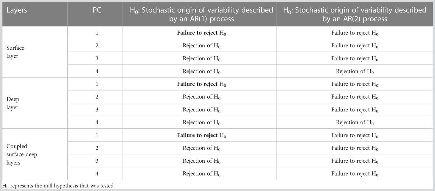
Table 2 Hypothesis test results for the stochastic origin of southern GoM variability, considering the first four principal components (PCs) for the separated and coupled EOF analyses.

The higher-order variability modes are not consistent with AR(1) processes (Table 2). These modes contain a more complex variability structure than the dominant ones, linear dynamics cannot explain them, and higher-order AR processes are needed to describe them. The different sources of southern GoM variability can be involved in such behavior, like surface-layer processes (e.g., atmosphere-ocean fluxes, advection and circulation of adjacent regions, and entrainment of sub-layers), a range of circulation features with a strong interaction between them (Zavala-Sansón et al., 2017; Guerrero et al., 2020), and topographic effects ruling to a certain extent the circulation throughout the water column (Pérez-Brunius et al., 2013; Zavala-Sansón, 2019). However, the higher-order variability can be adequately described using AR(2) processes, indicating that their dynamics is somewhat more complex than a linear one.

4 Discussion

This study explored different characteristics of southern GoM variability, providing realistic, robust, physically consistent, and statistically significant results. The choice of data and its processing were necessary to address the objectives posed for this work. Implementing climatological open boundary conditions (flow at the open boundaries without interannual variability) in the numerical simulation (Olvera-Prado et al., 2023) did not affect the reproducibility of southern GoM variability since it is mainly determined by wind stress (Gutiérrez de Velasco and Winant, 1996; DiMarco et al., 2005; Vázquez de la Cerda et al., 2005), eddy-driven vorticity fluxes (Vidal et al., 1992; Ohlmann et al., 2001; Meza-Padilla et al., 2019), and the bathymetry of the region (Pérez-Brunius et al., 2013; Zavala-Sansón, 2019). These processes were adequately implemented and represented in the numerical simulation (Olvera-Prado et al., 2023). This work did not address the variability occurring on the basin boundaries and that with spatial and temporal scales smaller than mesoscale, such as that associated with barotropic waves (Abolfazli et al., 2020; Gómez-Valdivia and Parés-Sierra, 2020).

This work used the EOFs technique to describe the mesoscale variability throughout the water column in the southern GoM by identifying its most important surface, deep, and coupled modes. Although the EOFs are not expected to identify individual dynamical modes (Storch and Zwiers, 1999; Monahan et al., 2009), they helped suggest a dynamical connection between surface and deep variability, including the timescales in which they are strongly connected. The findings of this work complement those of Pérez-Brunius et al. (2013), Hamilton et al. (2016), Hamilton et al. (2018), and Pérez-Brunius et al. (2018).

The coupling between surface and deep variability depends on the relative evolution of the deep layer with respect to the surface layer: it is maximal for the concurrent and quasi-concurrent states of deep variability, quasi-constant for previous states, and decreasing for subsequent states. The results suggest that deep dynamics is likely to influence the subsequent evolution of surface dynamics but do not demonstrate a causality relationship between them. A separation between the principal and higher-order coupled variability was found: the timescales and long-term persistence are mainly associated with deep dynamics for the principal variability, whereas higher-order variability has no clear association with surface or deep dynamics. The connection between the surface and deep layers is more complex than considering that due to the geographical isolation of the deep GoM from adjacent seas, the deep layer will evolve according to the surface layer’s behavior (Welsh and Inoue, 2000). The energy driving the deep circulation and dynamics comes from the surface layer; however, deep layer dynamics and the bathymetric configuration influence the dynamics and circulation throughout the water column in the southern GoM (Pérez-Brunius et al., 2013; Zavala-Sansón, 2019).

No vertical spatial correspondence between the surface and deep layers was found; the fluctuations of deep isopycnals do not mirror those of surface isopycnals. These results indicate that the circulation and dynamics throughout the water column in the southern GoM are more complex than those resulting from considering it as a two-layer system (Hamilton et al., 2018), in which, given the weak deep stratification, it is expected that the fluctuations of deep isopycnals mirror those of surface isopycnals. Thus, theoretical and simplified studies of the southern GoM using a two-layer system (e.g., Moreles et al., 2021) could be limited in adequately representing its variability and circulation patterns throughout the entire water column, being more appropriate to consider a more complex layer regime.

The principal coupled mode in the surface layer is described by a confined region in the southwest where the Campeche Gyre occurs. In the coupled EOF analysis of this work, that region was the only one statistically meaningful according to the PEV values; in the EOF analysis of Vázquez de la Cerda et al. (2005) using sea surface height anomalies, more statistically meaningful regions were obtained. This surface variability pattern is connected with deep variability in the center and a wide region in the north in the deep layer. These patterns only resulted in the coupled analysis using the data correlation matrix. Thus, they resulted from the intercorrelation between the surface and deep layers and are relevant to the dominant dynamics throughout the water column in the southern GoM. The finding of these patterns seems remarkable due to their very persistent nature (predictability timescale of 27.2 months) and possible connection with the Campeche Gyre dynamics (subsection 3.2). The influence of bathymetric characteristics (topographic control) on the development and evolution of the Campeche Gyre described by Pérez-Brunius et al. (2013) and Zavala-Sansón (2019) could be associated with the causal role of deep dynamics on surface dynamics suggested in this work. However, further research is needed to elucidate this relationship.

This work adds to those of Kolodziejczyk et al. (2011), Pérez-Brunius et al. (2013), and Pérez-Brunius et al. (2018) by providing the predictability timescales of the most important modes of southern GoM variability in terms of their decorrelation times. Using the decorrelation time to measure predictability produces well and robust results compared with other techniques, as Buckley et al. (2019) showed, and provides a proper interpretation of the persistence of a process (Trenberth, 1985; Storch and Zwiers, 1999). An application of the stochastic climate model of Hasselmann (1976) to the southern GoM was implemented. By coupling the surface ocean layer (the fast component of the system with a short memory) with a deep ocean layer (the slow component of the system with a long memory), the predictability timescale of the principal surface variability mode was extended to a much longer scale than that obtained by considering the layer separately, similar to what is done in coupled ocean-atmosphere studies (Grötzner et al., 1999, Dommenget and Latif, 2002; Moreles and Martínez-López, 2016). The predictability timescale of the principal variability mode in the surface layer was extended by a factor of 2.6, from 10.6 to 27.2 months, highlighting the persistent nature of this coupled pattern.

Strong evidence was provided for the stochastic origin of the dominant southern GoM variability throughout the water column. Despite the great variety of dynamical processes involved in southern GoM dynamics, its dominant variability can be described using linear dynamics in terms of the simplest AR process. The description of the higher-order variability in terms of the simplest AR process was prevented by different processes, among which the following are suggested: strong mesoscale dynamics, high-intensity variations of the fast component, short memory of the slow component, and weak surface-deep coupling. The nature of such processes could lead the long-term variability of a system to deviate from the stochastic null hypothesis of Hasselmann (1976), as found by Grötzner et al. (1999), Dommenget and Latif (2002), Moreles and Martínez-López (2016), and Buckley et al. (2019). The separation of the dynamics of the variability modes in a fast and a slow component implies that statistical models can be constructed to analyze their potential predictability (Storch and Zwiers, 1999); however, such construction is proposed for future research.

Applying EOF analysis in a coupled manner, as was done in this work, may help represent unknown deep variability in terms of known surface variability and eventually complement the development of ocean data assimilation systems throughout the water column by projecting surface information to deep layers in a statistically consistent manner (Chapman and Charantonis, 2017; Manucharyan et al., 2021; Sonnewald et al., 2021).

5 Conclusions

This work studied two major aspects of southern GoM dynamics: variability and predictability. It described the surface, deep, and coupled surface-deep variability of the southern GoM, its predictability timescales, and its stochastic origin. Relevant characteristics of the surface-deep coupling and dynamics of the southern GoM were provided. A strong connection was found between surface and deep variability, with particular and varied temporal and spatial characteristics related to the dominant circulation. The deep ocean’s role in generating long-term variability and its influence on the surface ocean’s behavior was described. This work adds support to the simplest stochastic model as a promising paradigm to approach variability and predictability in the climate system, emphasizing the utility of long-term free-running simulations and multivariate statistical analyses to address the variability and predictability of the climate system. Finally, it provides strong evidence for the stochastic origin of southern GoM variability, which has important implications for its description. We hope the methodology developed in this study can be improved and applied to other ocean basins.

This work provides further insights into the southern GoM dynamics and is complementary to others focusing on GoM dynamics; it also outlines some general implications for modeling, forecasting, and assimilation systems of the southern GoM. However, many questions remain to be answered, and further research using alternative and specific methodologies needs to be conducted to fully discern the GoM dynamics throughout the water column. An in-depth analysis of the dynamical connection throughout the water column in the southern GoM, specifically regarding the Campeche Gyre dynamics, is proposed for future research.

Data availability statement

Publicly available datasets were analyzed in this study. This data can be found here: The Zenodo repository [https://doi.org/10.5281/zenodo.5605092].

Author contributions

EM conceived and designed the study, acquired funding, analyzed and interpreted the data, created the figures, wrote and revised the manuscript, and approved the submitted version.

Funding

This work was supported by UNAM-PAPIIT IA104320 and by the Instituto de Ciencias del Mar y Limnología of the Universidad Nacional Autónoma de México (grant 626).

Acknowledgments

The author acknowledges Aurea De Jesús for her helpful discussions and valuable comments. Juan Nieblas-Piquero computed the monthly climatology of vertically averaged currents in the southern Gulf of Mexico, represented in Figure 3; Susana Higuera-Parra created Figure 1. The HYCOM simulation and its validation used in this study are a contribution of the Gulf of Mexico Research Consortium (CIGoM). The author thanks the reviewers for their valuable comments, which significantly improved this work.

Conflict of interest

The author declares that the research was conducted in the absence of any commercial or financial relationships that could be construed as a potential conflict of interest.

Publisher’s note

All claims expressed in this article are solely those of the authors and do not necessarily represent those of their affiliated organizations, or those of the publisher, the editors and the reviewers. Any product that may be evaluated in this article, or claim that may be made by its manufacturer, is not guaranteed or endorsed by the publisher.

References

Abolfazli E., Liang J.-H., Fan Y., Chen Q. J., Walker N. D., Liu J. (2020). Surface gravity waves and their role in ocean-atmosphere coupling in the Gulf of Mexico. J. Geophys. Res.: Oceans 125, e2018JC014820. doi: 10.1029/2018JC014820

CrossRef Full Text | Google Scholar

Adams C. M., Hernández E., Cato J. C. (2004). The economic significance of the Gulf of Mexico related to population, income, employment, minerals, fisheries and shipping. Ocean Coast. Manage. 47, 565–580. doi: 10.1016/j.ocecoaman.2004.12.002

CrossRef Full Text | Google Scholar

Box G., Jenkins G., Reinsel G., Ljung G. (2015). Time Series Analysis: Forecasting and Control. 5 edn (San Francisco: Wiley).

Google Scholar

Brooks C. (2019). Introductory Econometrics for Finance. 4 edn (Cambridge: Cambridge University Press). doi: 10.1017/9781108524872

CrossRef Full Text | Google Scholar

Buckley M. W., DelSole T., Lozier M. S., Li L. (2019). Predictability of north Atlantic Sea surface temperature and upper-ocean heat content. J. Climate 32, 3005–3023. doi: 10.1175/JCLI-D-18-0509.1

CrossRef Full Text | Google Scholar

Cassisi C., Montalto P., Aliotta M., Cannata A., Pulvirenti A. (2012). “Similarity measures and dimensionality reduction techniques for time series data mining,” in Advances in Data Mining Knowledge Discovery and Applications. Ed. Karahoca A. (Rijeka: IntechOpen). doi: 10.5772/49941

CrossRef Full Text | Google Scholar

Chapman C., Charantonis A. A. (2017). Reconstruction of subsurface velocities from satellite observations using iterative self-organizing maps. IEEE Geosci. Remote Sens. Lett. 14, 617–620. doi: 10.1109/LGRS.2017.2665603

CrossRef Full Text | Google Scholar

Cooley S., Schoeman D., Bopp L., Boyd P., Donner S., Ghebrehiwet D., et al. (2022). “Oceans and coastal ecosystems and their services,” in Climate Change 2022: Impacts, Adaptation and Vulnerability. Contribution of Working Group II to the Sixth Assessment Report of the Intergovernmental Panel on Climate Change. Eds. Pörtner H.-O., Roberts D. C., Tignor M., Poloczanska E. S., Mintenbeck K., Alegría A., et al. (Cambridge, UK and New York, NY, USA: Cambridge University Press), 379–550. doi: 10.1017/9781009325844.005

CrossRef Full Text | Google Scholar

CTOH (2013) Center for Topographic studies of the Ocean and Hydrosphere. What are Mesoscale Processes? Available at: http://ctoh.legos.obs-mip.fr/applications/mesoscale/what-are-mesoscale-processes (Accessed 2023-05-05).

Google Scholar

Cushman-Roisin B., Tang B., Chassignet E. P. (1990). Westward Motion of mesoscale eddies. J. Phys. Oceanogr. 20, 758–768. doi: 10.1175/1520-0485(1990)020<0758:WMOME>2.0.CO;2

CrossRef Full Text | Google Scholar

DelSole T. (2001). Optimally persistent patterns in time-varying fields. J. Atmospheric Sci. 58, 1341–1356. doi: 10.1175/1520-0469(2001)058<1341:OPPITV>2.0.CO;2

CrossRef Full Text | Google Scholar

DiMarco S. F., Nowlin W. D. Jr., Reid R. O. (2005). “A statistical description of the velocity fields from upper ocean drifters in the Gulf of Mexico,” in Circulation in the Gulf of Mexico: Observations and Models. Eds. Sturges W., Lugo-Fernandez A. (American Geophysical Union), 101–110. doi: 10.1029/161GM08

CrossRef Full Text | Google Scholar

Dommenget D., Latif M. (2002). Analysis of observed and simulated SST spectra in the midlatitudes. Climate Dynamics 19, 277–288. doi: 10.1007/s00382-002-0229-9

CrossRef Full Text | Google Scholar

Dubranna J., Pérez-Brunius P., López M., Candela J. (2011). Circulation over the continental shelf of the western and southwestern Gulf of Mexico. J. Geophys. Res.: Oceans 116, C08009. doi: 10.1029/2011JC007007

CrossRef Full Text | Google Scholar

Gil-Agudelo D. L., Cintra-Buenrostro C. E., Brenner J., González-Díaz P., Kiene W., Lustic C., et al. (2020). Coral reefs in the Gulf of Mexico large marine ecosystem: Conservation status, challenges, and opportunities. Front. Mar. Sci. 6. doi: 10.3389/fmars.2019.00807

CrossRef Full Text | Google Scholar

Gómez-Valdivia F., Parés-Sierra A. (2020). Seasonal upper shelf circulation along the central Western Gulf of Mexico: A preferential upcoast flow reinforced by the recurrent arrival of Loop Current eddies. J. Geophys. Res.: Oceans 125, e2019JC015596. doi: 10.1029/2019JC015596

CrossRef Full Text | Google Scholar

Grötzner A., Latif M., Timmermann A., Voss R. (1999). Interannual to decadal predictability in a coupled ocean–atmosphere general circulation model. J. Climate 12, 2607–2624. doi: 10.1175/1520-0442(1999)012<2607:ITDPIA>2.0.CO;2

CrossRef Full Text | Google Scholar

Guerrero L., Sheinbaum J., Mariño-Tapia I., González-Rejón J. J., Pérez-Brunius P. (2020). Influence of mesoscale eddies on cross-shelf exchange in the western Gulf of Mexico. Continental Shelf Res. 209, 104243. doi: 10.1016/j.csr.2020.104243

CrossRef Full Text | Google Scholar

Gutiérrez de Velasco G., Winant C. D. (1996). Seasonal patterns of wind stress and wind stress curl over the Gulf of Mexico. J. Geophys. Res.: Oceans 101, 18127–18140. doi: 10.1029/96JC01442

CrossRef Full Text | Google Scholar

Hamilton P., Bower A., Furey H., Leben R. R., Pérez-Brunius P. (2016). Deep Circulation in the Gulf of Mexico: A Lagrangian Study. (New Orleans, Louisiana Hamilton2016: U.S. Dept. of the Interior Bureau of Ocean Energy Management, Gulf of Mexico OCS Region), 289.

Google Scholar

Hamilton P., Leben R., Bower A., Furey H., Pérez-Brunius P. (2018). Hydrography of the Gulf of Mexico using autonomous floats. J. Phys. Oceanogr. 48, 773–794. doi: 10.1175/JPO-D-17-0205.1

CrossRef Full Text | Google Scholar

Hasselmann K. (1976). Stochastic climate models part i. theory. Tellus 28, 473–485. doi: 10.1111/j.2153-3490.1976.tb00696.x

CrossRef Full Text | Google Scholar

Judt F., Chen S. S., Curcic M. (2016). Atmospheric forcing of the upper ocean transport in the Gulf of Mexico: From seasonal to diurnal scales. J. Geophys. Res.: Oceans 121, 4416–4433. doi: 10.1002/2015JC011555

CrossRef Full Text | Google Scholar

Kolodziejczyk N., Ochoa J., Candela J., Sheinbaum J. (2011). Deep currents in the Bay of Campeche. J. Phys. Oceanogr. 41, 1902–1920. doi: 10.1175/2011JPO4526.1

CrossRef Full Text | Google Scholar

Manucharyan G. E., Siegelman L., Klein P. (2021). A deep learning approach to spatiotemporal Sea surface height interpolation and estimation of deep currents in geostrophic ocean turbulence. J. Adv. Modeling Earth Syst. 13, e2019MS001965. doi: 10.1029/2019MS001965

CrossRef Full Text | Google Scholar

Martínez-López B., Zavala-Hidalgo J. (2009). Seasonal and interannual variability of cross-shelf transports of chlorophyll in the Gulf of Mexico. J. Mar. Syst. 77, 1–20. doi: 10.1016/j.jmarsys.2008.10.002

CrossRef Full Text | Google Scholar

Meza-Padilla R., Enríquez C., Liu Y., Appendini C. M. (2019). Ocean circulation in the Western Gulf of Mexico using self-organizing maps. J. Geophys. Res.: Oceans 124, 4152–4167. doi: 10.1029/2018JC014377

CrossRef Full Text | Google Scholar

Monahan A. H., Fyfe J. C., Ambaum M. H. P., Stephenson D. B., North G. R. (2009). Empirical orthogonal functions: The medium is the message. J. Climate 22, 6501–6514. doi: 10.1175/2009JCLI3062.1

CrossRef Full Text | Google Scholar

Monreal-Gómez M., Salas-de León D. (1997). “Circulación y estructura termohalina del Golfo de México,” in Contribuciones a la Oceanografía Física en México, Monografía, vol. 3 . Ed. Lavín-Peregrina M. (Unión Geofísica Mexicana), 183–199.

Google Scholar

Moreles E., Martínez-López B. (2016). Analysis of the simulated global temperature using a simple energy balance stochastic model. Atmósfera 29, 279–297. doi: 10.20937/ATM.2016.29.04.01

CrossRef Full Text | Google Scholar

Moreles E., Zavala-Hidalgo J., Martínez-López B., Ruiz-Angulo A. (2021). Influence of Stratification and Yucatan Current Transport on the Loop Current Eddy Shedding Process. J. Geophys. Res.: Oceans 126, e2020JC016315. doi: 10.1029/2020JC016315

CrossRef Full Text | Google Scholar

Morey S. L., Gopalakrishnan G., Sanz E. P., Souza J. M. A. C. D., Donohue K., Pérez-Brunius P., et al. (2020). Assessment of numerical simulations of deep circulation and variability in the Gulf of Mexico using recent observations. J. Phys. Oceanogr. 50, 1045–1064. doi: 10.1175/JPO-D-19-0137.1

CrossRef Full Text | Google Scholar

Morey S. L., Zavala-Hidalgo J., O’Brien J. J. (2005). “The seasonal variability of continental shelf circulation in the northern and Western Gulf of Mexico from a high-resolution numerical model,” in Circulation in the Gulf of Mexico: Observations and Models. Eds. Sturges W., Lugo-Fernandez A. (American Geophysical Union), 203–218. doi: 10.1029/161GM16

CrossRef Full Text | Google Scholar

Muller-Karger F. E., Smith J. P., Werner S., Chen R., Roffer M., Liu Y., et al. (2015). Natural variability of surface oceanographic conditions in the offshore Gulf of Mexico. Prog. Oceanogr. 134, 54–76. doi: 10.1016/j.pocean.2014.12.007

CrossRef Full Text | Google Scholar

NASEM (2018). National Academies of Sciences, Engineering, and Medicine. (Washington, DC: The National Academies Press). doi: 10.17226/24823

CrossRef Full Text | Google Scholar

NOAA (2008). National ocean service. Gulf of Mexico at a Glance (Washington, D.C., U.S: Depart­ment of Commerce, National Oceanic and Atmospheric Administration), 30.

Google Scholar

North G. R., Bell T. L., Cahalan R. F., Moeng F. J. (1982). Sampling errors in the estimation of empirical orthogonal functions. Monthly Weather Rev. 110, 699–706. doi: 10.1175/1520-0493(1982)110<0699:SEITEO>2.0.CO;2

CrossRef Full Text | Google Scholar

Ohlmann J. C., Niiler P. P., Fox C. A., Leben R. R. (2001). Eddy energy and shelf interactions in the Gulf of Mexico. J. Geophys. Res.: Oceans 106, 2605–2620. doi: 10.1029/1999JC000162

CrossRef Full Text | Google Scholar

Olvera-Prado E. R., Moreles E., Zavala-Hidalgo J., Romero-Centeno R. (2023). Upper–lower layer coupling of recurrent circulation patterns in the Gulf of Mexico. J. Phys. Oceanogr. 53, 533–550. doi: 10.1175/JPO-D-21-0281.1

CrossRef Full Text | Google Scholar

Pérez-Brunius P., Furey H., Bower A., Hamilton P., Candela J., García-Carrillo P., et al. (2018). Dominant circulation patterns of the deep Gulf of Mexico. J. Phys. Oceanogr. 48, 511–529. doi: 10.1175/JPO-D-17-0140.1

CrossRef Full Text | Google Scholar

Pérez-Brunius P., García-Carrillo P., Dubranna J., Sheinbaum J., Candela J. (2013). Direct observations of the upper layer circulation in the southern Gulf of Mexico. Deep Sea Res. Part II: Topical Stud. Oceanogr. 85, 182–194. doi: 10.1016/j.dsr2.2012.07.020

CrossRef Full Text | Google Scholar

Portela E., Tenreiro M., Pallas-Sanz E., Meunier T., Ruiz-Angulo A., Sosa-Gutiérrez R., et al. (2018). Hydrography of the central and Western Gulf of Mexico. J. Geophys. Res.: Oceans 123, 5134–5149. doi: 10.1029/2018JC013813

CrossRef Full Text | Google Scholar

Schmitt R. W. (2018). The ocean’s role in climate. Oceanography 31, 32–40. doi: 10.5670/oceanog.2018.225

CrossRef Full Text | Google Scholar

Sonnewald M., Lguensat R., Jones D. C., Dueben P. D., Brajard J., Balaji V. (2021). Bridging observations, theory and numerical simulation of the ocean using machine learning. Environ. Res. Lett. 16, 073008. doi: 10.1088/1748-9326/ac0eb0

CrossRef Full Text | Google Scholar

Storch H. V., Zwiers F. W. (1999). Statistical Analysis in Climate Research (Cambridge: Cambridge University Press). doi: 10.1017/CBO9780511612336

CrossRef Full Text | Google Scholar

Thomson D. (1982). Spectrum estimation and harmonic analysis. Proc. IEEE 70, 1055–1096. doi: 10.1109/PROC.1982.12433

CrossRef Full Text | Google Scholar

Trenberth K. E. (1985). Persistence of daily geopotential heights over the southern hemisphere. Monthly Weather Rev. 113, 38–53. doi: 10.1175/1520-0493(1985)113<0038:PODGHO>2.0.CO;2

CrossRef Full Text | Google Scholar

Vázquez de la Cerda A. M., Reid R. O., DiMarco S. F., Jochens A. E. (2005). “Bay of Campeche circulation: An update,” in Circulation in the Gulf of Mexico: Observations and models. Eds. Sturges W., Lugo-Fernandez A. (American Geophysical Union), 279–293. doi: 10.1029/161GM20

CrossRef Full Text | Google Scholar

Vidal V. M. V., Vidal F. V., Pérez-Molero J. M. (1992). Collision of a Loop Current anticyclonic ring against the continental shelf slope of the western Gulf of Mexico. J. Geophys. Res.: Oceans 97, 2155–2172. doi: 10.1029/91JC00486

CrossRef Full Text | Google Scholar

Vukovich F. M. (2007). Climatology of ocean features in the Gulf of Mexico using satellite remote sensing data. J. Phys. Oceanogr. 37, 689–707. doi: 10.1175/JPO2989.1

CrossRef Full Text | Google Scholar

Welsh S. E., Inoue M. (2000). Loop Current rings and the deep circulation in the Gulf of Mexico. J. Geophys. Res.: Oceans 105, 16951–16959. doi: 10.1029/2000JC900054

CrossRef Full Text | Google Scholar

Wilks D. (2019). Statistical Methods in the Atmospheric Sciences. 4 edn (Elsevier Science).

Google Scholar

Yoskowitz D., Leon C., Gibeaut J., Lupher B., Lopez M., Santos C., et al. (2013). Gulf 360: State of the Gulf of Mexico (Texas: Harte Research Institute for Gulf of Mexico Studies, Texas A&M University-Corpus Christi), 52.

Google Scholar

Zavala-Hidalgo J., Morey S. L., O’Brien J. J. (2003). Seasonal circulation on the western shelf of the Gulf of Mexico using a high-resolution numerical model. J. Geophys. Res.: Oceans 108, 3389. doi: 10.1029/2003JC001879

CrossRef Full Text | Google Scholar

Zavala-Sansón L. (2019). Nonlinear and time-dependent equivalent-barotropic flows. J. Fluid Mechanics 871, 925–951. doi: 10.1017/jfm.2019.354

CrossRef Full Text | Google Scholar

Zavala-Sansón L., Pérez-Brunius P., Sheinbaum J. (2017). Point source dispersion of surface drifters in the southern Gulf of Mexico. Environ. Res. Lett. 12, 024006. doi: 10.1088/1748-9326/aa537c

CrossRef Full Text | Google Scholar