Recognition and location of marine animal sounds using two-stream ConvNet with attention

There are abundant resources and many endangered marine animals in the ocean. Using sound to effectively identify and locate them, and estimate their distribution area, has a very important role in the study of the complex diversity of marine animals (Hanny et al., 2013). We design a Two-Stream ConvNet with Attention (TSCA) model, which is a two-stream model combined with attention, in which one branch processes the temporal signal and the other branch processes the frequency domain signal; It makes good use of the characteristics of high time resolution of time domain signal and high recognition rate of frequency domain signal features of sound, and it realizes rapid localization and recognition of sound of marine species. The basic network architecture of the model is YOLO (You Only Look Once) (Joseph et al., 2016). A new loss function focal loss is constructed to strengthen the impact on the tail class of the sample, overcome the problem of data imbalance and avoid over fitting. At the same time, the attention module is constructed to focus on more detailed sound features, so as to improve the noise resistance of the model and achieve high-precision marine species identification and location. In The Watkins Marine Mammal Sound Database, the recognition rate of the algorithm reached 92.04% and the positioning accuracy reached 78.4%.The experimental results show that the algorithm has good robustness, high recognition accuracy and positioning accuracy.

1 Introduction

In recent years, the development of marine resources has been paid more and more attention by countries all over the world. The sea area is vast and the resource reserve is huge. Marine animals are complex and diverse, and many marine creatures exchange information with sound, such as whales can rely on sound to socialize and locate their prey; There are many endangered mammals in the sea, and their identification and positioning through sound is an effective means of protection for them. For example, maintaining the number of large whales is crucial to marine ecology, and restoring the number of baleen whales and sperm whales can strengthen the health of the global marine ecological ecosystem. Therefore, using passive acoustic classification and species positioning technology to effectively identify them and estimate their distribution areas has a very important role and research significance in the study of the complex diversity of marine animals. Through this technology, we can reveal the behavior and species density of marine animals. However, due to unknown statistical characteristics and low signal to noise ratio (SNR) conditions, marine mammal voice recognition and localization may be the most challenging task in the field of animal bioacoustics. Therefore, it is a hot spot problem in this field to effectively identify and then estimate the distribution area.

At present, there are two main methods for marine mammal voice recognition: one is classification based on spectral characteristics. (Nanaware et al., 2014) manually classifies the sounds of six marine mammals through the extracted energy and spectral cross-correlation coefficients. (André et al., 2011) identified whether there was a whale voice in the audio by detecting the unique frequency bandwidth of the whale voice, with an accuracy rate of 90%. These methods have good classification effect when there are few marine animals, but it is difficult to distinguish some species with similar sound spectrum. Because marine mammals can emit a variety of different sounds, it is also difficult to identify. Another method is to use machine learning method to classify. This kind of method can identify some sounds that cannot be classified by the spectrum map. (Ibrahim et al., 2016) extracted Mel Frequency Cepstral Coefficients (MFCC) and Discrete Wavelet Transform (DWT) coefficients of whale sounds in the North Atlantic Ocean, and used Support Vector Machine (SVM) to classify their sounds. Experiments show that the method is better than using spectral coefficients to classify their sounds. (González-Hernández et al., 2017) uses 1/6 octave and feedforward neural network to identify eleven species, and each species emits a variety of sounds, such as whistling, shouting and squeaking. The model shows good performance and achieves a classification rate of 90% with low computational cost. (Brown and Smaragdis, 2009) uses MFCC as a feature to classify the sounds of killer whales through hidden Markov model and Gaussian mixture model, achieving 90% recognition rate; (Lu et al., 2021) applies feature fusion method, and uses MFCC, Linear Frequency Cepstral Coefficient (LFCC) and time-domain feature fusion as feature parameters for voice recognition But this method is not effective in low SNR environment; (Mingtuo and Wenyu, 2019) used AlexNet and transfer learning methods to automatically detect and classify killer whales, long fin pilot whales and harp seals with extensive overlapping living areas, and achieved good results, with certain limitations, and the calculation process was cumbersome.

There are three main methods of sound source location: TDE or TDOA, depth learning, and sound energy First of all, the method based on TDE or TDOA is to calculate the time delay or phase difference of sound arriving at different acoustic sensors, and estimate the arrival azimuth of the sound source under the condition that the geometry of the array is known. A typical algorithm is phase transformation (GCC-PHAT) (Pérez-Rubio, 2021; Yoshizawa, 2021), This kind of method is limited by time synchronization, and has poor practicability and high cost.

The method based on depth learning mainly focuses on the sound source localization of supervised learning (Yang et al., 2018; Yangzhou et al., 2019; Jin et al., 2020). The deep neural network is trained by extracting acoustic data features, such as amplitude and phase, collected from different acoustic sensors The cost of this kind of location method system is also very large, which seriously restricts the universality of the location system.

The method based on sound energy is direct and effective (Sheng and Hu, 2004; Dranka and Coelho, 2015; Bo, 2022). However, its effectiveness depends on the propagation attenuation model of sound energy. It is often assumed that the sound energy has a linear attenuation relationship with the propagation distance, which is not true in most real scenes.

It can be seen from the above analysis that these studies are all aimed at the classification of one or several marine mammal audio signals, which cannot fully describe the complex and variable characteristics of sound, and cannot be used to identify more marine mammal species. It is difficult to obtain high recognition accuracy in the case of complex environmental noise. At the same time, these identification algorithms do not provide location information, and cannot estimate the distribution area of marine organisms, nor can they further reveal the behavior and population density of marine animals.

Therefore, we have designed a Two Stream ConvNet with Attention (TSCA) for fast sound recognition and location of marine animal sound features. This model decomposes sound signals into time domain signals and frequency domain signals. One branch of the dual stream network processes time signals and the other branch processes frequency domain signals; The basic network architecture of the two independent streams is YOLO. The model suppresses environmental noise through attention, and realizes information fusion. Finally, the model completes the rapid and accurate identification and location of the sound of marine species.

2 Materials and methods

2.1 Data collection

1) Marine animal sound data set

The voice recognition data set is The Watkins Marine Mammal Sound Database, which contains about 1654 records and 1654 spectrograms, recording more than 31 kinds of marine mammals, and the duration of each sample is 3~20s. 24 filters are selected to extract CMFCC features of sound signals. In order to improve the robustness of identifying sound sources in complex environments, Gaussian noise with different signal-to-noise ratios (SNR) is added to the recording samples to expand the data. SNR is respectively - 30db, - 15db, 0db, 15db and 30db.

2) Locate Dataset

Because it is difficult to obtain marine species positioning data sets, we use different human voices to replace the voice of marine species. The voice of people is recorded at a distance of 1km from the three recording sensors. The number of men and women with different timbre is 50, and the sensor spacing is 1m. The number of different recording samples for each person is 30, and the voice in the recording samples is stable, and the voice duration is 5~10s. Considering the existence of various noises in the marine environment, Gaussian noises with different SNR are added to the above recording samples to expand the data, so as to generalize the performance of the system and improve the robustness of identifying sound sources in complex environments. The SNR is respectively - 30db, - 15db, 0db, 15db and 30db. At this time, the number of samples is 3000 × 5 = 15000. Add 5000 groups of soundless source sounding test sets, a total of 20000 test samples.

2.2 Sound processing of marine animals

The sound of marine animals includes static, non static and quasistatic noises (Suleman and Ura, 2007). In order to reduce the influence of background noise, it is necessary to preemphasis the sound signal from the background noise. From the overall perspective, the acoustic signal will change every other period of time, and it is not a steady process. But in a certain period of time, it has a certain degree of stability. This part is usually called a frame. For the global call signal, the final analysis is the time series parameters obtained from each frame.

2.2.1 Preemphasis

Affected by the radiation of the animal’s mouth, nose and lip, the call signal collected by the sensor will lose energy, and the high-frequency part (above 800Hz) will fall according to the octave. The high-frequency resolution is low, which affects the recognition results (Yi, 2000). Preemphasis can increase the amplitude of high frequency and reduce the influence of background noise by utilizing the characteristic difference between noise and signal.

In order to compensate for the loss of high-frequency components, the audio signal is pre weighted using Finite Impulse Response (FIR) filter. Formula of the FIR filter $H$is shown in Formula (2.1).

$\begin{array}{ll}H(z)=1-a{z}^{-1}& \text{(2.1)}\end{array}$

Where, Z is the transfer function parameter, the value of $a$is close to and slightly less than 1.

When the value of $a$ is 0.98, the amplitude frequency and phase frequency characteristics of the pre emphasis filter are shown in Figure 1. Figure 2 is the Fin whale sound signal graph before and after the pre emphasis processing.

FIGURE 1

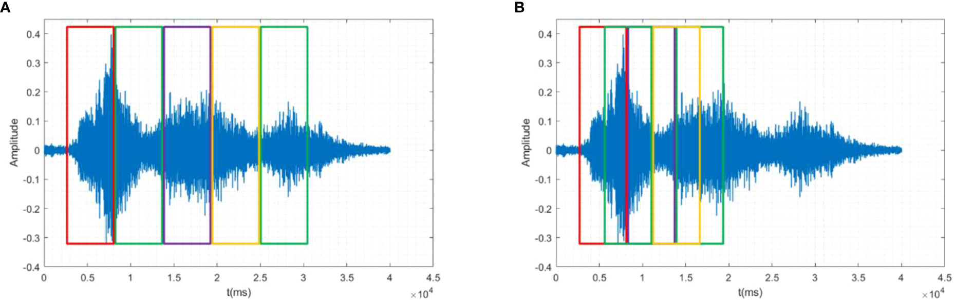
Figure 1 Amplitude frequency and phase frequency characteristic diagram of pre emphasis filter, (A) Amplitude frequency characteristic diagram, (B) Phase frequency characteristic diagram.

FIGURE 2

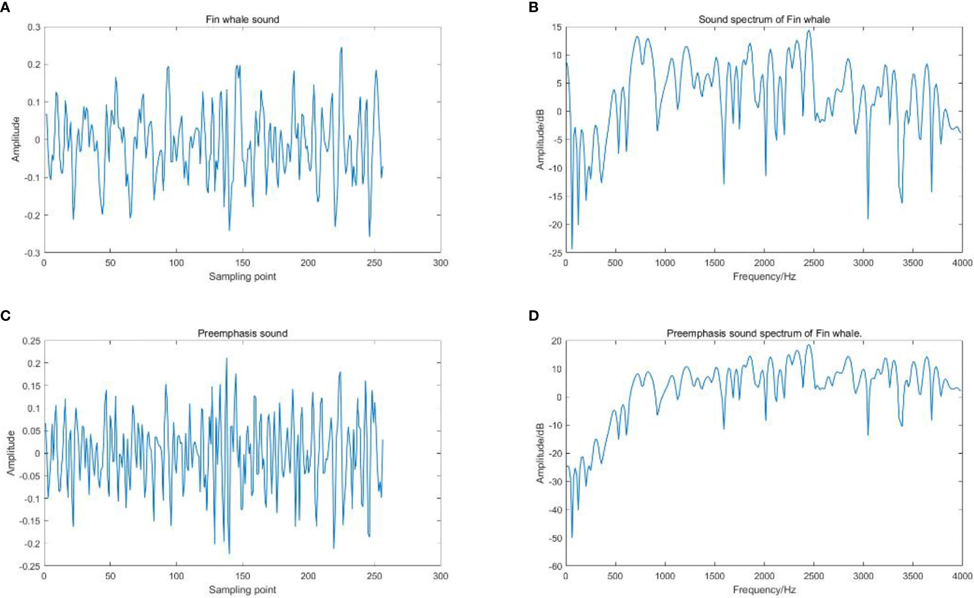
Figure 2 The Fin whale sound signal graph before and after the pre emphasis processing, (A) Fin whale sound, (B) Sound spectrum of Fin whale, (C) Preemphasis sound of Fin whale, (D) Preemphasis sound spectrum of Fin whale.

It can be seen from Figure 2 that before pre weighting, the time domain waveform of fin whale calls is relatively discrete, and after pre weighting, it is relatively concentrated and stable. In addition, the low frequency part of the acoustic signal is restrained to some extent, and the middle and high frequency part is effectively improved. The compensation effect of high-frequency loss is good, which is conducive to subsequent feature extraction and recognition.

2.2.2 Framing and windowing

Animal signal is a non-stationary time-varying sound signal, which is easily interfered and affected by vocal production, surrounding environment, vocal tract characteristics and system factors. But in a very short time range (10~30ms), it is considered to be stable. Through a specific window function, the voice signal is windowed and divided into frames for 10~30ms. Each segment is an analysis frame, referred to as a frame for short. Continuous and overlapping are two common framing methods, as shown in Figure 3. To ensure smooth transition between successive frames, we choose overlapping segmentation method. In this algorithm, the sampling frequency of the signal is 22kHz, the frame length is 440 data points, and the corresponding time is 20ms; To ensure the positioning accuracy, 200 points are moved from the frame, and the corresponding time is 10ms.

FIGURE 3

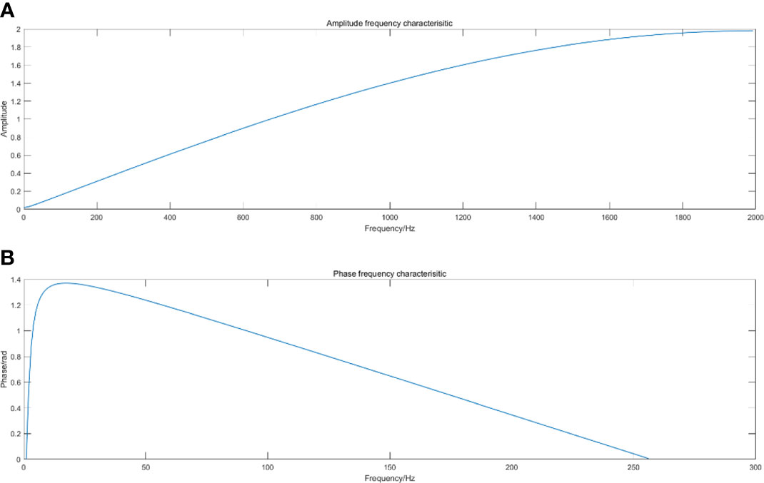
Figure 3 Schematic diagram of framing and windowing, (A) Continuous framing, (B) Overlapping framing.

After framing, in order to make the speech signal globally continuous, and make each frame show some features of periodic function to facilitate subsequent feature extraction, windowing is required. The window function $w(n)$ selected in this paper is Hamming window function, which can be expressed as Eq. (2.2):

$\begin{array}{ll}w(n)=\{\begin{array}{c}0.54-0.46\cos (\frac{2\pi n}{T-1}) , 0\ll n\ll T-1\\ 0 , other\end{array}& \text{(2.2)}\end{array}$

Where, T is the length of a frame signal.

The signal before windowing is expressed as $a(n)$, and the signal after windowing is $s(n)$, as shown in Formula 2.3:

$\begin{array}{ll}s(n)=w(n)a(n)& \text{(2.3)}\end{array}$

2.2.3 CMFCC(compound mel-frequency cepstrum coefficient)

CMFCC is Frequency domain characteristics of marine animal sounds. It has been proved that the frequency domain feature CMFCC is the feature with the best recognition rate in voice recognition applications. The extraction method of CMFCC is shown in (Hu et al., 2022). First, the preprocessed signal s (n) is transformed into FFT (Fast Fourier Transformation), its logarithmic energy spectrum is convolved with the filter bank and inversion filter in Meyer frequency domain respectively, and then the output vector is transformed into discrete cosine to obtain CMFCC characteristics. The calculation formula is Eq.2.4. Figure 4 shows the CMFCC characteristics of the orcinus orca’s voice.

FIGURE 4

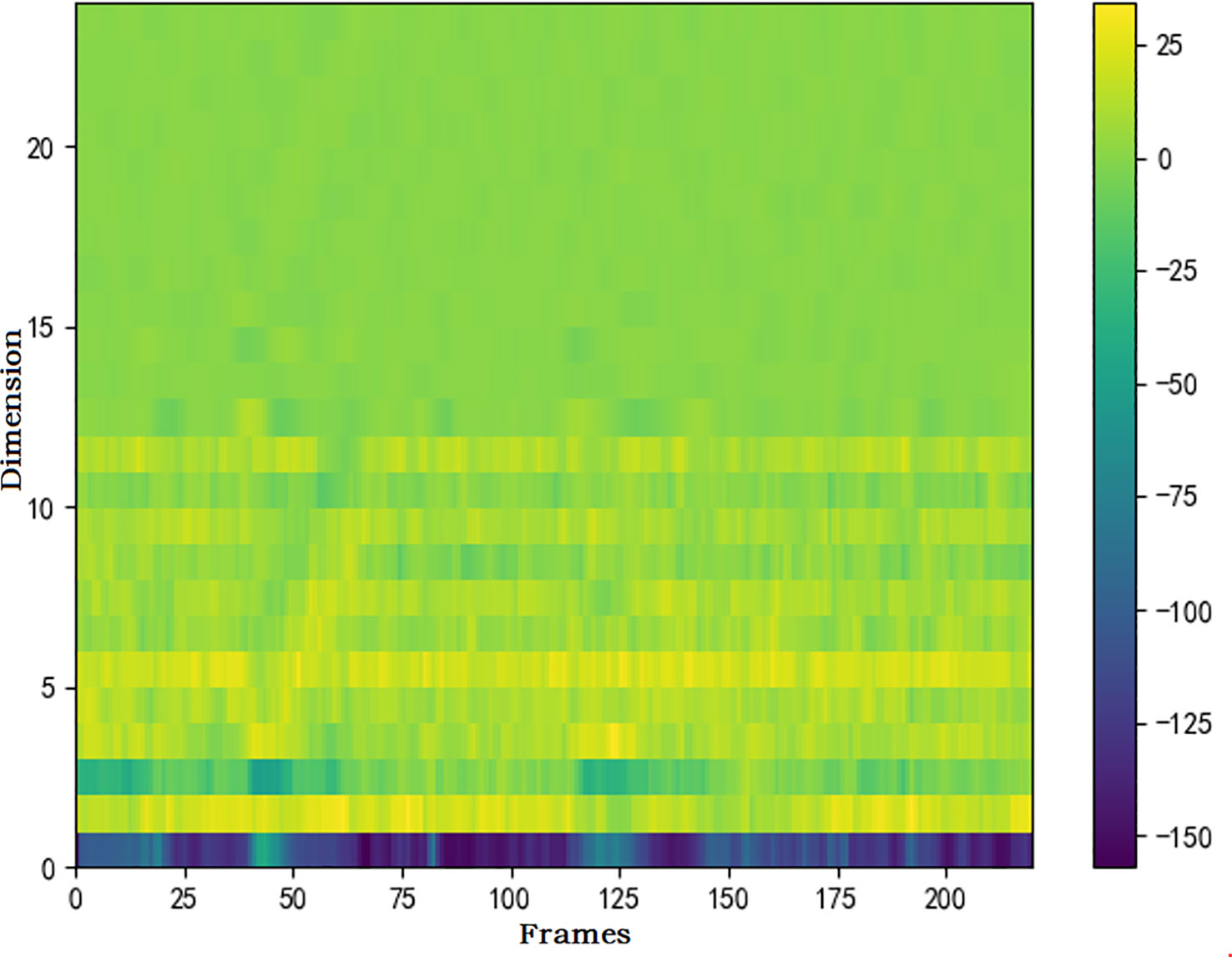
Figure 4 The CMFCC characteristics of the orcinus orca’s voice.

$\begin{array}{ll}CMFCC(i,j)=\sqrt{\frac{2}{M}}{\sum }_{m=0}^{m-1}\text{log}[S(i,m)]\text{cos}(\frac{\pi j(2m+1)}{2M})& \text{(2.4)}\end{array}$

Where, $CMFCC(i,j)$ is the CMFCC of the i-th frame signal, M is the number of filter banks and inversion filters in the Mel frequency domain, j is the number of CMFCCs, and $S(i,m)$ is the power spectrum in the Mel frequency domain.

2.3 TDOA

The estimation location method based on Time Difference of Arrival (TDOA) has the characteristics of small computation, good real-time, and strong practicability (Benesty et al. 2008). The TDOA method is divided into two steps. First, calculate the time difference (time delay estimation) of the sound source signal arriving at the microphone array, and then establish the sound source location model through the geometry of the microphone array and solve it to obtain the location information (location estimation). As shown in Figure 5, the coordinate axes $x$, $y$ and $z$ in the figure represent the space distance.

FIGURE 5

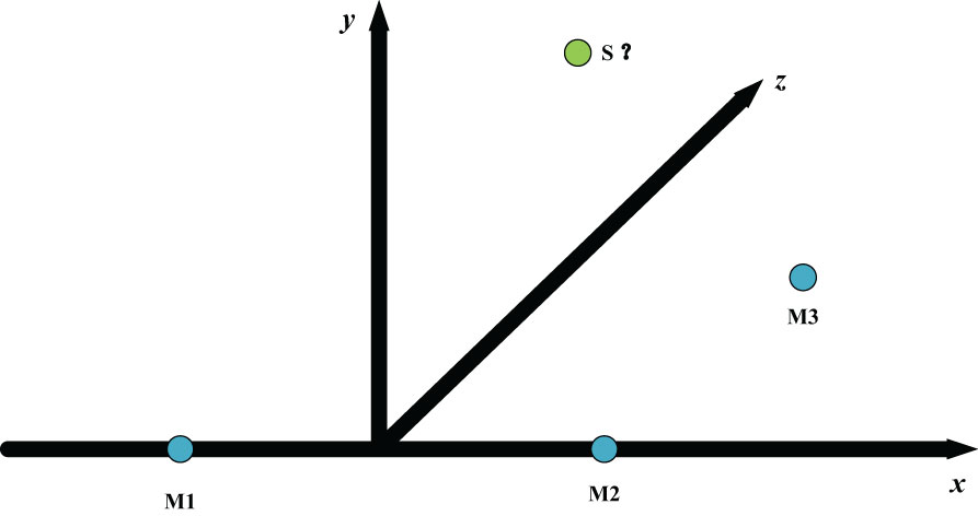
Figure 5 The sound source and Microphone array M1, M2, M3.

We assume that there is a sound source in the space (denoted as $s(t)$, indicates the position of sound source in space at time $t$), two microphones (denoted as m1 and m2, their positions in the space are M1 and M2 respectively, and the received signals are $x_1(t)$ and $x_2(t)$. Then the signals received by microphones m1 and m2 are shown in Eq.2.5.

$\begin{array}{ll}\{\begin{array}{c}{x}_1(t)=s(t-{\tau }_1)+n_1(t)\\ x_2(t)=s(t-{\tau }_2)+n_2(t)\end{array}& \text{(2.5)}\end{array}$

Where, ${\tau }_1$ and ${\tau }_2$ is the delay time for the sound source to reach the two microphones, respectively. $n_1(t)$ and $n_2(t)$ are additive noises. Then the time delay of sound source signal arriving at two microphones is $\tau$,as shown in Eq.2.6.

$\begin{array}{ll}\tau ={\tau }_1-{\tau }_2& \text{(2.6)}\end{array}$

Here, ${\tau }_1$ and ${\tau }_2$ is obtained through the positioning coordinates of TSCA.

We set three microphones to receive the sound signal, and determine the position coordinates of the sound source in the two-dimensional plane. Since the sound of marine animals we detected belongs to the far-field model, the waveform of the sound source arriving at the microphone array is regarded as a plane wave. Therefore, we can calculate the Direction of Arrival (DOA) through the sound signals collected by microphones at two positions. As shown in Figure 6.

FIGURE 6

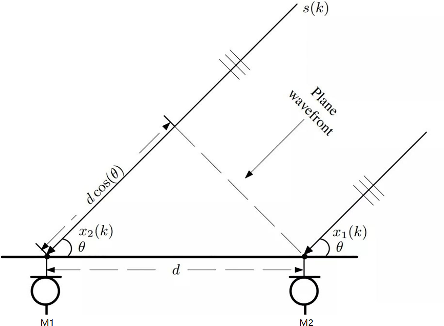
Figure 6 Far-field positioning model.

According to the geometric relationship of the microphone array, we can determine the angle of the sound source relative to the microphone array $\theta$, as shown in Eq.2.7.

$\begin{array}{ll}\theta =arccos\frac{C\widehat{\tau }}{d}& \text{(2.7)}\end{array}$

Where, $\widehat{\tau }$Is the estimated time delay, $d$ is the distance between two sensors, and c is the speed of sound.

Two azimuth angles $\theta$ can be obtained by measuring the values of three microphones. The Chan algorithm (Chan and Ho, 1994) solves the position (x, y) of marine animals using Eq.2.8.

$\begin{array}{ll}\left[\begin{array}{c}x\\ y\end{array}\right]=-[\begin{array}{cc}{x}_{2,1}& y_{2,1}\\ x_{3,1}& y_{3,1}\end{array}]*\left\{\left[\begin{array}{c}{R}_{2,1}\\ R_{3,1}\end{array}\right]R_1+\frac{1}{2}\left[\begin{array}{c}{R}_{2,1}^2-K_2+K_1\\ R_{3,1}^2-K_3+k_1\end{array}\right]\right\}& \text{(2.8)}\end{array}$

Where, $K_1=x_1^2+y_1^2$, $K_2=x_2^2+y_2^2$, $K_3=x_3^2+y_3^2$, $R_1=\sqrt{{(x_1-x)}^2+{(y_1-y)}^2}$, $R_{2,1}=dcos({\theta }_1)$, $R_{3,1}=dcos({\theta }_2)$, ${\theta }_1$ is the azimuth angle of the sound source relative to the microphone M1 and M2, ${\theta }_2$ is the azimuth angle of the sound source relative to the microphone M1 and M3.

2.4 Two-stream ConvNet with attention

Two stream convolutional network appeared in 2014, and it has made considerable progress in the research of action recognition, temporal and spatial behavior detection (Simonyan and Zisserman, 2014).

We adopted the idea of Two Stream ConvNet, and designed a Two Stream ConvNet with Attention (TSCA) for fast voice recognition and location of marine animal voice features. The model structure is shown in Figure 7. TSCA uses YOLO net as the basic framework. By embedding time, channel, and space convolution module (TCS), the multi-dimensional network expansion is realized, which improves the model’s anti noise ability, and also improves the detection and positioning accuracy of the algorithm.

FIGURE 7

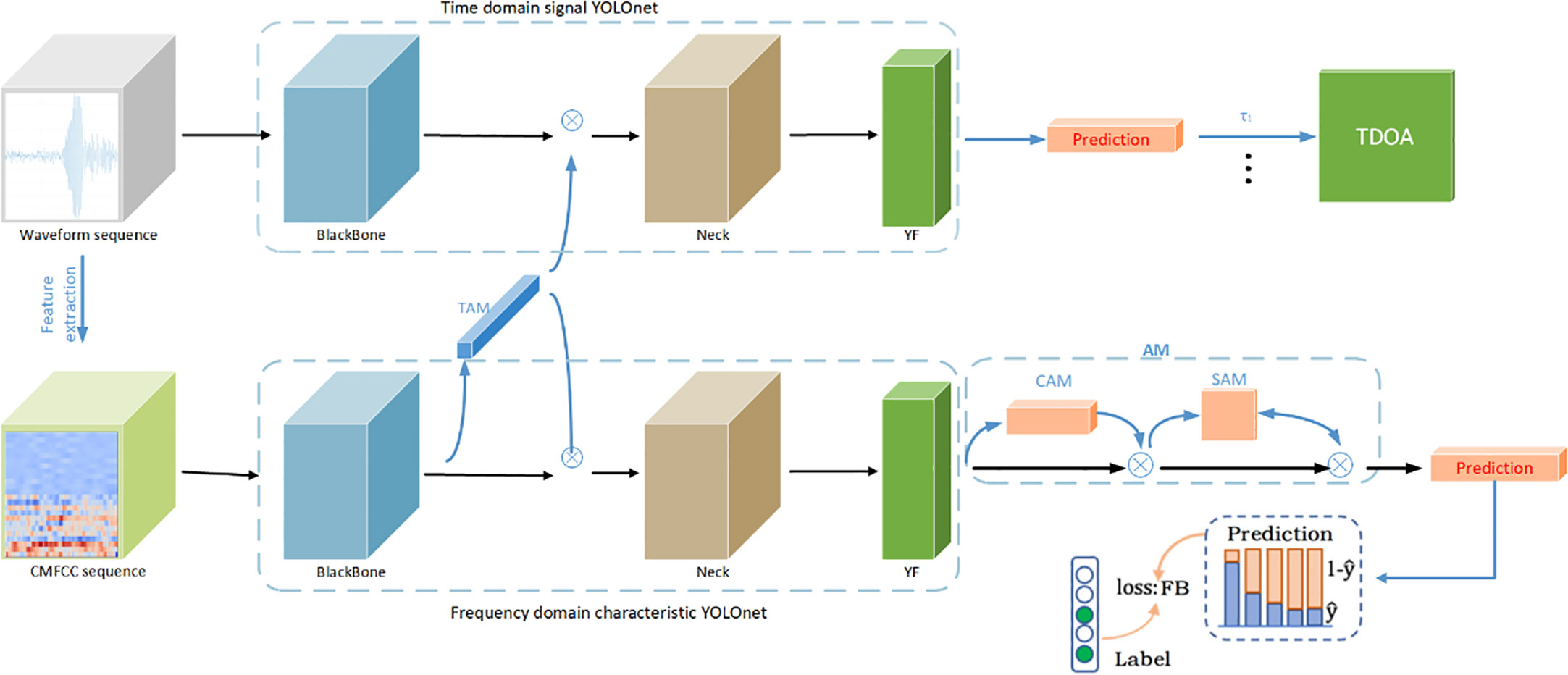
Figure 7 TSCA model structure.

YOLO net is a fast and high recognition rate target detection and recognition algorithm and network model, which realizes end to end target detection. The anchor box is used to combine the regression problem of classification and target location. It achieves high efficiency, flexibility and good generalization performance. Our goal is to quickly determine the position of marine animals while realizing sound recognition, so we choose YOLO5 as the basic network structure of TSCA.

YOLO net of frequency domain features realizes accurate recognition of marine animal calls through CMTCC feature sequences; YOLO net in time domain uses the high time resolution of call sequence signal to achieve accurate sound location. Since the data frames of the two streams are the same, we fuse the time information of CMFCC channel to YOLO net in the time domain through Time Attention (TAM) after the BackBone of YOLO net to improve the positioning accuracy of YOLO net in the time domain; At the same time, channel and spatial attention are added after the feature layer of the frequency domain feature YOLO net output to improve the anti noise ability of the model.

For the loss function, the two classification cross entropy loss function is fused. Improve the focus loss function to reduce the weight of head class data in the loss function and increase the weight of tail class in the loss function to solve the problem of low accuracy caused by tail data. At the same time, the model combines TDOA module to achieve voice positioning.

2.5 Space time attention module

Attention mechanism has better automatic regulation effect on noise (Ma et al., 2021; Senwei et al., 2021; Zhao et al., 2021). We use attention modules TAM, CAM, SAM (TCS) in the model, as shown in Figure 7. In TCS, channel, time and space information is focused by maximizing and averaging pooling of channels, time and space.

After the BackBone of YOLO net, the time information of CMFCC channel is fused to YOLO net in the time domain through the TAM module. The attention TAM is used to change the weight of each frame time dimension of the time domain YOLO net to achieve dual stream network information fusion, so as to improve the positioning accuracy of YOLO net in the time domain.

In order to better solve the problem of “what” and “where”, we draw on the ideas of Convolutional Block Attention Module (CBAM). We use Channel Attention Module (CAM) to focus on “what” in the network; Use the Spatial Attention Module (SAM) to focus on “where” in the network, as shown in Figure 8.

FIGURE 8

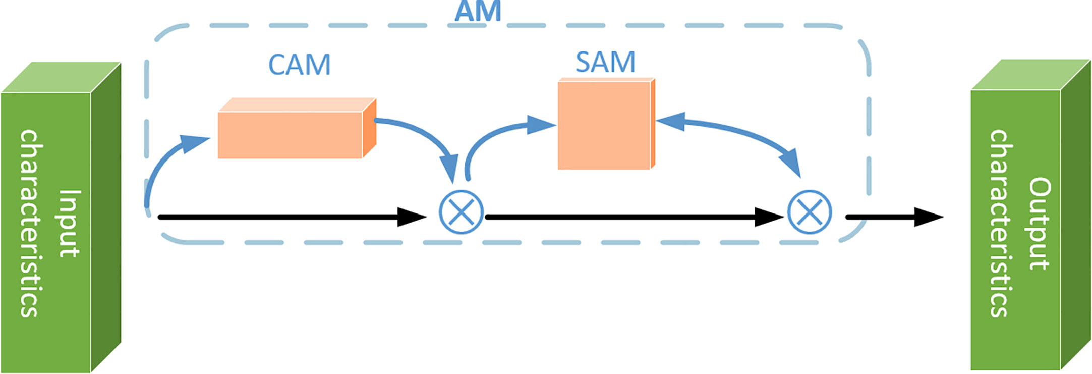
Figure 8 Attention module (Channel, Space convolutional block attention module).

Assume that the input characteristic graph is $F\in R^{C\times H\times W}$, the channel attention diagram is $M_c$. The spatial attention map is $M_s$. The formulas of channel attention and spatial attention are as follows Eq.2.9 and Eq.2.10:

$\begin{array}{ll}{F}^{\prime }=M_c(F)\otimes F& \text{(2.9)}\end{array}$

$\begin{array}{ll}{F}^{″}=M_s(F^{\prime })\otimes F^{\prime }& \text{(2.10)}\end{array}$

Where, $M_c\in R^{C\times 1\times 1}$, $M_s\in R^{1\times H\times W}$, $\otimes$ represents element by element multiplication. In the process of element by element multiplication, attention value will also be propagated to the next level.

2.6 Focus loss function

In the experiment, we found that there was a serious data imbalance problem in the time-space oriented data set of marine animal calls. The distribution of species category tagging data is shown in Figure 9. In the training process of the model, the prediction of the model will be biased towards the head class, making the error rate of the tail class prediction increase.

FIGURE 9

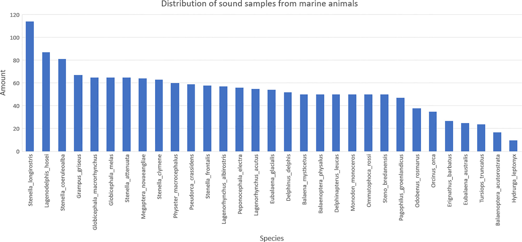
Figure 9 The distribution of species category tagging data.

In classification tasks, the binary cross entropy loss function (BCE Loss) is usually used as the loss function of multi label classification. However, BCE Loss did not take into account the difference between the contributions of the head and tail classes in the long tail data, resulting in low accuracy of model training.

We get a new loss function Focal BCE Loss (FB) by combining the focus loss function (Lin et al., 2017) (Focal Loss) and BCE Loss, as shown in Eq.2.13, to reduce the weight of the head loss function in multi label data and increase the weight of the tail loss function in multi label data.

$\begin{array}{ll}\text{A}=-\alpha L{(1-\widehat{y})}^{\gamma }L(\widehat{y})y& \text{(2.11)}\end{array}$

$\begin{array}{ll}\text{B}=(1-\text{α}){\widehat{y}}^{\text{γ}}\text{L}(1-\widehat{y})(1-\text{y})& \text{(2.12)}\end{array}$

$\begin{array}{ll}\text{FB}=\text{A}-\text{B}& \text{(2.13)}\end{array}$

Where, A represents the Focal Loss, B represents the BCE, L represents the natural logarithmic function, α represents the weighting factor, α∈ [0,1], positive class is α, Negative class is 1- α, Y represents the correct label. $\widehat{y}$ represents the probability of y=1, $\widehat{y}$ ∈(0,1). γ is the focus parameter, ${(1-\widehat{y})}^{\text{γ}}$ is the modulation factor.

When $\widehat{y}$ →0, modulation factor ${(1-\widehat{y})}^{\text{γ}}$ will be close to 1, so the weight of correct classification will increase.

When $\widehat{y}$ →1, modulation factor ${(1-\widehat{y})}^{\text{γ}}$ will be close to 0, and the weight for correct classification will decrease.

By adjusting the focus parameters γ to reduce the weight of samples that are easy to classify.

When γ= 0, FB is equivalent to BCE Loss. Along with γ Increase of, modulation factor ${(1-\widehat{y})}^{\text{γ}}$. The influence of, γ= 5. The effect is the best.

With the increase of γ, the influence of modulation factor ${(1-\widehat{y})}^{\text{γ}}$ will also increase. The experiment found that, γ= 5, the model has the best effect.

3 Results

3.1 Model parameters

Stochastic Gradient Descent (SGD) optimizer is used for model training. Kinetic energy is set to 0.9, weight attenuation is set to 0.00001, initial learning rate is set to 0.075, and epoch is set to 40.

3.2 Loss function analysis

The $\text{γ}$ value of the loss function FB is related to the imbalance degree of the data set. In order to analyze the influence of focusing parameter $\text{γ}$ in FB on the model detection results, we set different focusing parameter $\text{γ}$, from 0.1 to 10. Here, we use Mean Average Precision (mAP) as the evaluation index to measure the advantages and disadvantages of the algorithm. The experimental result are shown in Figure 10. The solid line represents the reference line, that is, the detection result of the model using BCE loss function, mAP is 83.61%. The dot represents the test result of using FB in the model, and the dotted line is the sixth degree polynomial fitting curve of the dot. The horizontal axis data represents different values of focusing parameter $\text{γ}$ from 0.1 to 10. It can be seen that when $\text{γ}$=5, the model detection result reaches 92.04% of the optimal result of $\text{γ}$; $\text{γ}$ ∈ [0,2], the model test result mAP increases the fastest. When $\text{γ}$>6, the model test result mAP starts to decline. We can see the effectiveness of the loss function FB in solving long tail data.

FIGURE 10

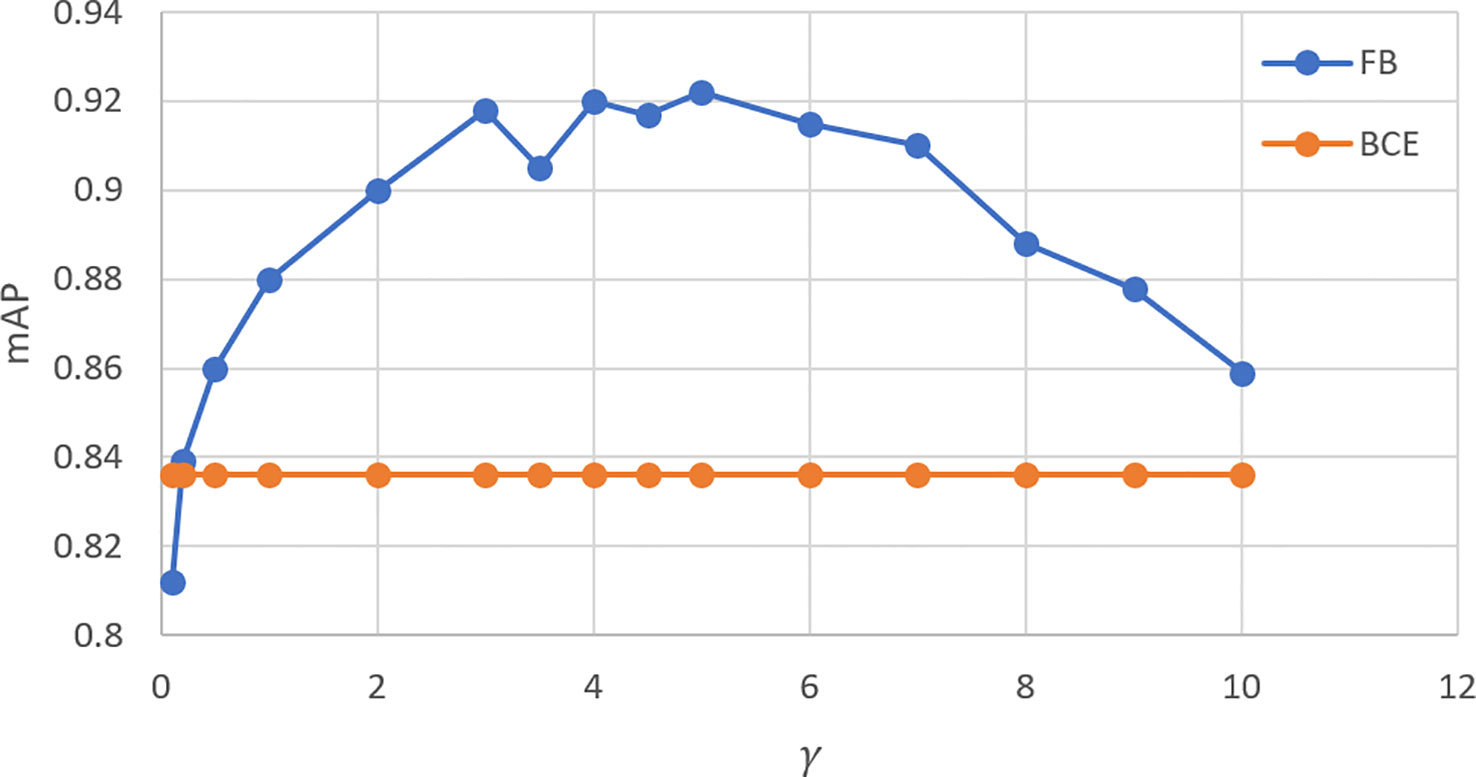
Figure 10 mAP of the model when parameter γ of FB takes different values.

3.3 Attention module analysis

In order to verify the effect of spatiotemporal attention module TCS on sound recognition of marine animals, TAM, CAM, SAM, and 3D TCS were added to YOLO net respectively in the experiment. The experimental results of a noise dataset are shown in Table 1. TAM, CAM, SAM, and TCS are represented by T, C, S, and TCS respectively. The line without FB represents the detection results of the above four attention modules added to TSCA respectively. It can be found that after adding TCS, the mAP of the model is the highest. Compared with the benchmark test result of 83.61%, the mAP is increased by 6.43%, followed by the TAM, which is increased by 4.48%.

TABLE 1

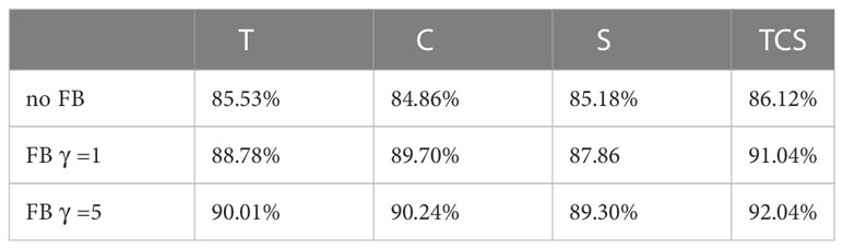
Table 1 Model detection results of various attention modules (mAP).

3.4 Comparison of call classification

1) In order to compare the recognition accuracy of different models under different classifiers, Support Vector Machine (SVM), K Nearest Neighbors (KNN) and Random Forest (RF) are also selected for classification and the results are compared. In order to obtain relatively objective results, 50% of the samples in each experiment are randomly selected as the training set, and the recognition rate is the average of 10 experiments. The identification results of a noise dataset are shown in Table 2.

TABLE 2

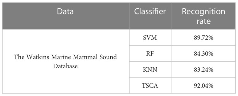
Table 2 Classification results of different classifiers.

It can be seen from Table 2 that when using the same feature parameters, the recognition rate of TSCA model is better than the other two classifiers, indicating that TSCA has better recognition performance.

2) Due to the complexity of the marine environment, in order to further verify the robustness of the model in this paper, data with different SNR are tested. The recognition rate is the average of 10 experiments. The recognition results are shown in Figure 11.

FIGURE 11

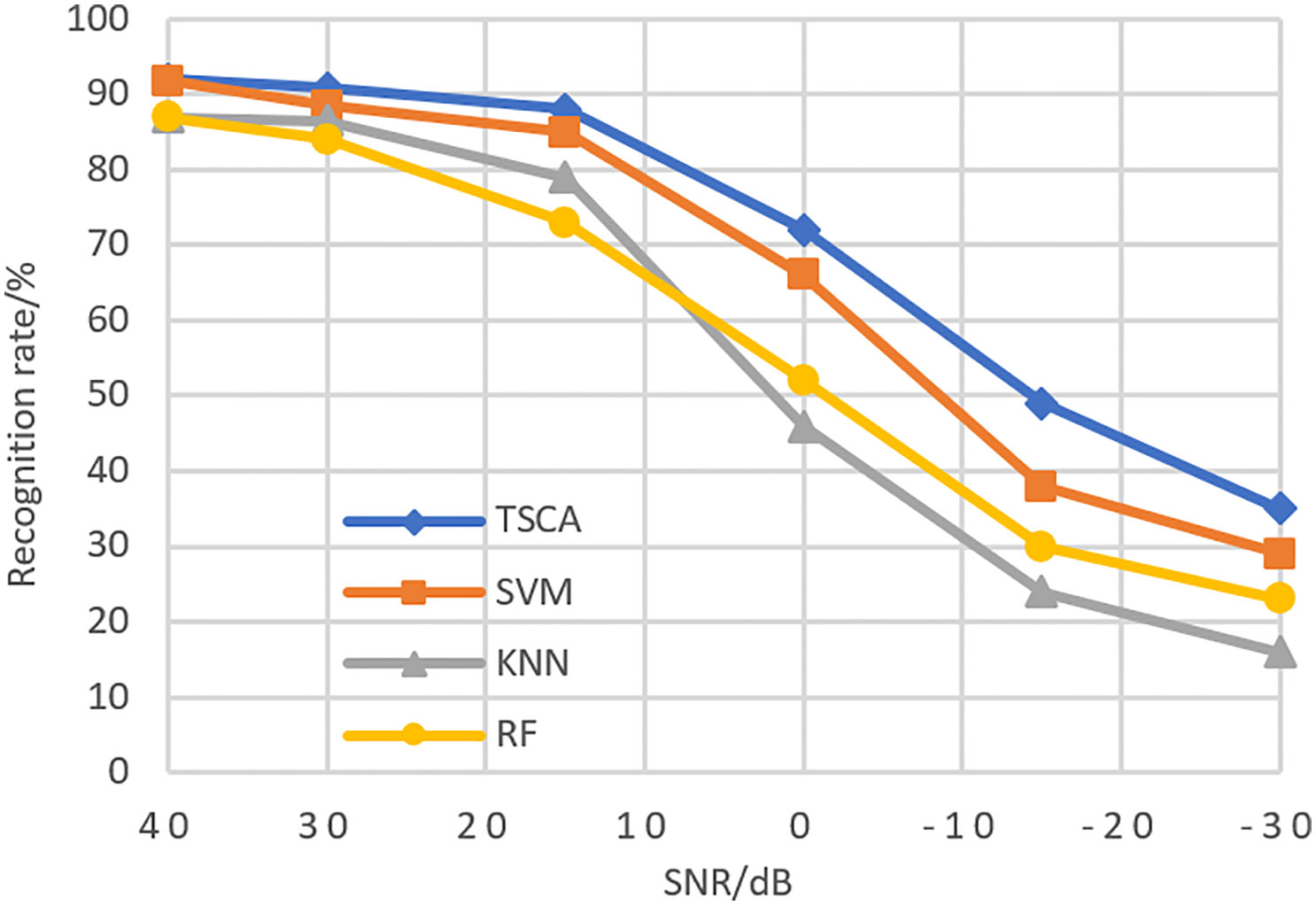
Figure 11 Recognition rate of different models under different SNR.

It can be seen from Figure 11 that in the process of gradual reduction of the signal-to-noise ratio, the TSCA model has the most gentle decline, which indicates that the TSCA model has good anti noise robustness in the marine environment.

3.5 Positioning

At present, the commonly used technologies for sound source localization products are TDOA, MUSIC and BP neural network sound source localization algorithms. The test samples are self built sample sets. Table 3 summarizes the positioning accuracy of TSCA model and the above algorithms in different environments. Since the positioning accuracy is less than 20% when the SNR is negative, it is not indicated in the table. The test set used for verification is 5000 in total, including 2000 groups of test samples of silent source sound.

TABLE 3

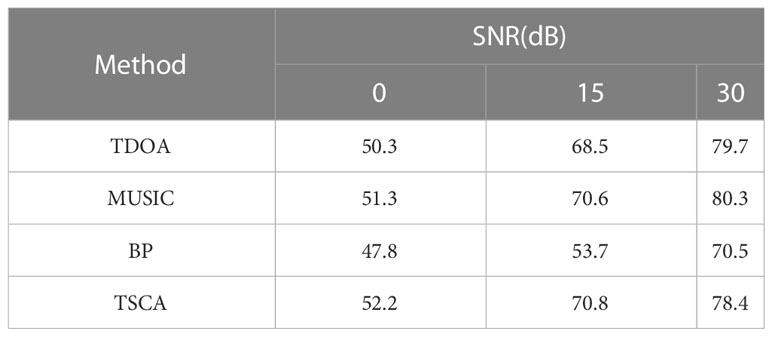
Table 3 The accuracy comparison of algorithms in different environments.

4 Discussion

From Table 2 and Figure 11, we can see that the TSCA model introduces the spatiotemporal attention module TCS and the FB loss function to solve the problem of data heterogeneity (long tail phenomenon). The recognition rate of TSCA model is better than other algorithms in the case of no noise and noise. It shows that the TSCA model can achieve good recognition results in the recognition of the call of marine species.

According to the data in Table 3, although the maximum positioning accuracy of MUSIC and TDOA algorithms is 80.3% and 79.7% respectively. However, the minimum positioning accuracy of both is less than 52%, which is a very significant gap compared with the optimal effect. The reason is that it is difficult to set a threshold parameter for both algorithms, so the peak value of the estimator will shift slightly at the correct position under different conditions. Therefore, the algorithm may not have the best localization accuracy for sound sources with different SNR.

Our TSCA model has higher positioning accuracy than the common BP algorithm under any same conditions. When TSCA is at 0db or 15db, the positioning accuracy is significantly higher than other algorithms. It shows that the TSCA model has good anti-noise ability and can achieve high positioning accuracy in marine species location.

5 Conclusion

The recognition and research of marine organisms’ sound is a very important and meaningful work. By recognizing and tracking marine animal targets through sound, it is possible to accurately grasp the distribution, growth status, and behavioral characteristics of marine animals. There are many endangered marine animals in the sea, which can be effectively identified by sound and their distribution areas can be estimated, which plays a very important role in the study of the complex diversity of marine animals. At present, the recognition and classification technology of marine animal sounds largely depends on acoustic characteristics, such as MFCC, LPC, STFT, etc., and classification models, such as GMM, SVM, etc. These recognition technologies can not fully describe the complex and variable characteristics of sound, and often perform poorly. Most of these recognition technologies are used to classify one or several marine animal audio signals. It is impossible to recognize more marine mammal species, and it is impossible to judge the position and distance of marine organisms based on sound.

Therefore, we design a TSCA model to deal with such problems. This model is a dual stream model algorithm based on YOLO net and attention. The algorithm realizes fast localization and recognition of marine species sound from the time high resolution of time domain signal features and the high classification accuracy of frequency domain features. The model uses the loss function FB to strengthen the influence on the tail class of the sample, improve the data imbalance, avoid the over fitting problem, and achieve good results; At the same time, it embeds TAM to achieve dual stream integration; Through TAM, SAM and CAM attention modules, the model can pay attention to more detailed sound features, improve the noise resistance of the model, and achieve high-precision sound recognition and positioning of marine species. The experimental results show that the algorithm has good performance and great practical application potential.

Data availability statement

The original contributions presented in the study are included in the article/supplementary material. Further inquiries can be directed to the corresponding authors.

Author contributions

All authors listed have made a substantial, direct, and intellectual contribution to the work and approved it for publication.

Funding

This research is supported by Chengdu Science and Technology Program (2022-YF09-00019-SN), Sichuan Science and Technology Program (2022NSFSC0020, 2023NSFSC1926), and the Chengdu Research Base of Giant Panda Breeding (NO. 2020CPB-C09, NO. 2021CPB-B06).

Conflict of interest

The authors declare that the research was conducted in the absence of any commercial or financial relationships that could be construed as a potential conflict of interest.

Publisher’s note

All claims expressed in this article are solely those of the authors and do not necessarily represent those of their affiliated organizations, or those of the publisher, the editors and the reviewers. Any product that may be evaluated in this article, or claim that may be made by its manufacturer, is not guaranteed or endorsed by the publisher.

References

André M., van der Schaar M., Zaugg S., Houegnigan L., Sanchez A. M., Castell J. V., et al. (2011). Listening to the deep: live monitoring of ocean noise and cetacean acoustic signals. Mar. Pollut. Bull. 63 (1-4), 18–26. doi: 10.1016/j.marpolbul.2011.04.038

PubMed Abstract | CrossRef Full Text | Google Scholar

Benesty J, Chen J, Huang Y (2008). Micrphone array processing. Berlin, Heidelberg

Google Scholar

Bo X. (2022). Single sound source localization and tracking technology based on sound energy (Guangzhou University) Guangzhou, China.

Google Scholar

Brown J. C., Smaragdis P. (2009). Hidden Markov and Gaussian mixture models for automatic call classification. J. Acoustical Soc. America 125 (6), EL221. doi: 10.1121/1.3124659

CrossRef Full Text | Google Scholar

Chan Y. T., Ho K. C. A. (1994)Simple and efficient estimator for hyperbolic location. signal processing (Accessed IEEE Transactions).

Google Scholar

Dranka E., Coelho R. F. (2015). Robust maximum likelihood acoustic energy based source localization in correlated noisy sensing environments. IEEE J. Selected Topics Signal Process. 9 (2), 259–267. doi: 10.1109/JSTSP.2014.2385657

CrossRef Full Text | Google Scholar

González-Hernández F. Rubén, Sánchez-Fernández L. P., Suárez-Guerra S., Sánchez-Pérez L. A. (2017). Marine mammal sound classification based on a parallel recognition model and octave analysis. Appl. Acoustics. 119, 17–28. doi: 10.1016/j.apacoust.2016.11.016

CrossRef Full Text | Google Scholar

Hanny D. E., Delarue J., Mouy X., Martin B. S., Leary D., Oswald J. N., et al. (2013). Marine mammal acoustic detections in the northeastern chukchi Sea, September 2007-July 2011. Continental Shelf Res. 67, 127–146. doi: 10.1016/j.csr.2013.07.009

CrossRef Full Text | Google Scholar

Hu S. X., Liao Z. W., Hou R., Chen P. (2022) Characteristic sequence analysis of giant panda voiceprint. Front. Phys. 10, 839699. doi: 10.3389/fphy.2022.839699

CrossRef Full Text | Google Scholar

Ibrahim A. K., Zhuang H., Erdol N., et al. (2016)A new approach for north atlantic right whale upcall detection[C] (Accessed Xi’an: International Symposium on Computer, Consumer and Control).

Google Scholar

Jin L., Yan J., Du X., Xiao X. C., Fu D. Y. (2020). RNN for solving time-variant generalized Sylvester equation with applications to robots and acoustic source localization. IEEE Trans. Ind. Inf. 16 (10), 6359–6369. doi: 10.1109/TII.2020.2964817

CrossRef Full Text | Google Scholar

Joseph R., Santosh D., Ross G., Ali F. (2016). You only look once: unified, real-time object detection (Las Vegas, NV, USA: CVPR), 779–788. doi: 10.48550/arXiv.1506.02640

CrossRef Full Text | Google Scholar

Lin T. Y., Goyal P., Girshick R., et al. (2017)Focal loss for dense object detection (Accessed Proceedings of the IEEE international conference on computer vision).

Google Scholar

Lu T., Han B., Yu F. (2021). Detection and classification of marine mammal sounds using AlexNet with transfer learning. Ecol. Inf. 62. doi: 10.1016/j.ecoinf.2021.101277

CrossRef Full Text | Google Scholar

Ma H. W., Liu G. C., Yuan Y. (2021)Enhanced non-local cascading network with attention mechanism for hyperspectral image denoising (Accessed International Conference on Acoustics Speech and Signal Processing ICASSP).

Google Scholar

Mingtuo ZHONG, Wenyu C. A. I. (2019). “Marine mammal sound recognition based on feature fusion,” in Electronic sci. & tech. (Electronic Science and Technology: Xi An, China) 30

Google Scholar

Nanaware S., Shastri R., Joshi Y., et al. (2014)Passive acoustic detection and classification of marine mammal vocalizations[C], lucknow (Accessed International Conference on Communication and Signal Processing).

Google Scholar

Pérez-Rubio M. C. (2021). Dynamic adjustment of weighted GCC-PHAT for position estimation in an ultrasonic local positioning system. Sensors 21 (21), 7051. doi: 10.3390/s21217051

PubMed Abstract | CrossRef Full Text | Google Scholar

Senwei L., ZhongZhen H., Mingfu L., Haizhao Y. (2021)Instance enhancement batch normalization: an adaptive regulator batch noise (Accessed AAAI Conference on Artificial Intelligence).

Google Scholar

Sheng X., Hu Y. H. (2004). Maximum likelihood multiple-source localization using acoustic energy measurements with wireless sensor networks. IEEE Trans. Signal Process. 53 (1), 44–53. doi: 10.1109/TSP.2004.838930

CrossRef Full Text | Google Scholar

Simonyan K., Zisserman A. (2014). “Two-stream convolutional networks for action recognition in videos,” in Advances in neural information processing systems. NIPS 2014: Montreal, CANADA, 27 27.

Google Scholar

Springer (2008). Micrphone array processing.

Google Scholar

Suleman M., Ura T. (2007)Vocalization based individual classification of humpback whales using support vector machine (Accessed Oceans).

Google Scholar

Yang X., Li Y., Sun Y., et al. (2018)Fast and robust RBF neural network based on global K- means clustering with adaptive selection radius for sound source angle estimation (Accessed IEEE Transactions on Antennas and Propagation).

Google Scholar

Yangzhou J., Ma Z., Huang X. (2019). A deep neural network approach to acoustic source localization in a shallow water tank experiment. J. Acoustical Soc. America 146 (6), 4802–4811. doi: 10.1121/1.5138596

CrossRef Full Text | Google Scholar

Yi K. (2000). Speech signal processing (Beijing, China: National Defense Industry Press), 10–70.

Google Scholar

Yoshizawa S. (2021). Underwater acoustic localization based on IR-GCC-PHAT in reverberant environments. Int. J. Circuits 15, 164–171. doi: 10.46300/9106.2021.15.18

CrossRef Full Text | Google Scholar

Zhao Y., Zhai D., Jiang J., Liu X. (2021). ADRN: attention-based deep residual network for hyperspectral image denoising (Barcelona, Spain: International Conference on Acoustics Speech and Signal Processing ICASSP), 2668–2672.

Google Scholar