 Lu-Sha Yu
 Hailun He
 Hengling Leng
 Hailong Liu2,4
- 1State Key Laboratory of Satellite Ocean Environment Dynamics, Second Institute of Oceanography, Ministry of Natural Resources, Hangzhou, China
- 2State Key Laboratory of Numerical Modeling for Atmospheric Sciences and Geophysical Fluid Dynamics, Institute of Atmospheric Physics, Chinese Academy of Sciences, Beijing, China
- 3Southern Marine Science and Engineering Guangdong Laboratory, Zhuhai, China
- 4College of Earth and Planetary Sciences, University of Chinese Academy of Sciences, Beijing, China
This paper investigates the interannual variability of January sea surface temperature (SST) in the Amundsen Sea (AS) during the period 1982–2022. SST in the Pine Island Bay (PIB) is found to exhibit the most significant interannual variation, with a standard deviation up to 0.6°. Composite analysis indicates that, in warmer years, the January SST at PIB is approximately 1° higher on average than that in cooler years, and its variation in warmer (cooler) years corresponds to lower (higher) sea ice concentration (SIC) and more (less) surface heat flux; the latter factor is primarily influenced by the albedo of SIC. Further analysis suggests that variability in January SIC is largely dominated by northward sea ice motion during the previous November (r = −0.82), which is consistent with the presence of a contemporaneous northerly 10 m wind anomaly trigged by the Amundsen Sea Low (ASL). The ASL-associated northerly wind anomaly drives northward sea ice motion, reduces SIC, and thus increases the downward heat flux that ultimately results in warmer SST, and vice versa. This study identifies the possible mechanism of anomalous January SST in the PIB, which could provide an important clue for seasonal forecasts of summer SST in the AS.
Introduction
More and more attentions are focused on the Southern Ocean in recent years, especially the West Antarctic Amundsen Sea (AS; Figure 1) has great importance for future global sea level rise and regional and even global climate variability. (i) In recent decades, the mass of the West Antarctic Ice Sheet has declined dramatically, corresponding to an increase in global mean sea level of approximately 7 mm between 1992 and 2017, in which the Pine Island Glacier of the AS has dominated regional contributions (approximately 40%; Payne et al., 2004; Rignot et al., 2019; Morlighem et al., 2020). Furthermore, the glaciers of the AS are currently retreating and thinning at faster rates than other regions in Antarctica, suggesting the warming signal of the AS (Pritchard et al., 2012; Paolo et al., 2015; Rignot et al., 2019). (ii) The Antarctic sea ice (ASI) as a whole experienced a dramatic reversal in the entire 1979–2018 record, in which ASI showed an expansion trend during 1979 to 2014, and began decline precipitously since then (Parkinson, 2019; Eayrs et al., 2021). Different from the positive trends in the Ross Sea, the Indian Ocean and the Weddell Sea, sea ice in the AS has shown negative trends in each month, with its highest seasonal trend being in summer at −14300 ± 2600 km2 yr−1 (Parkinson and Cavalieri, 2012; Hobbs et al., 2015), which could be linked to the warming trend of sea surface temperature (SST) in the AS.
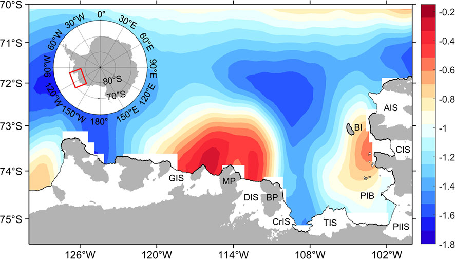
Figure 1 Map of the Amundsen Sea (red rectangle in inset map), showing mean sea surface temperature (color shading) in January averaged over 41 years (1982–2022). Floating glacial ice (ice shelves) is shown in white. Black labels indicate ice shelves (PIIS, Pine Island Ice Shelf; TIS, Thwaites Ice Shelf, AIS, Abbot Ice Shelf; CIS, Cosgrove Ice Shelf; CrIS, Crosson Ice Shelf; DIS, Dotson Ice Shelf; GIS, Getz Ice Shelf) and other topographic features (PIB, Pine Island Bay; MP, Martin Peninsula; BP, Bear Peninsula; and BI, Burke Island).
SST of the polar regions play an important role for the sea ice formation, sea ice melt and the heat exchange between the ocean and atmosphere (Key et al., 1997). What’s more, SST has the potential to influence the ocean circulation through its impact to the density (Lhardy et al., 2021). In the context of global warming, unlike the Arctic, the Southern Ocean as a whole experienced a weak cooling trend in SST (e.g., Comiso, 2000; Lebedev, 2007; Maheshwari et al., 2013). However, recent studies indicate that SST in the AS has exhibited a significant warming trend during the periods from 1950–2000, 1979–2012, 1982–2009 and 1982–2011 (Oza et al., 2011; Maheshwari et al., 2013; Purich et al., 2018; Zhang et al., 2019), with high temperature increases and warming rates (e.g., Bromwich et al., 2013). This decades-long SST warming trend plays an important role in the rapid shrinking of sea ice in the AS, and has led to a precipitous decline of Antarctic sea ice since 2014 (Parkinson, 2019; Eayrs et al., 2021). In addition, using NOAA optimum interpolation SST data from 1982 to 2011, Maheshwari et al. (2013) found SST anomalies in the Southern Ocean showed interannual variability, which was related to the El Nino/La Nina events, and pointed out that the AS experienced relatively warmer SST during 1992 and 1997, and colder SST during 1999 and 2000, without further discussion. Thus, more detailed description and the mechanism on this interannual variation of SST in the AS require further investigation.
SST in the AS also has unique ecological effects. It is well known that due to its high abundance of iron, the Amundsen Sea Polynya (ASP) has the highest net primary production of any Antarctic polynya (Arrigo et al., 2012; Arrigo et al., 2015) and thus has relatively high chlorophyll-a (Chla) concentrations (Arrigo and Van Dijken, 2003). Recent research found that SST exerted a strong influence on Chla concentration; indeed, the correlation between them is strongest in the AS, with a maximum correlation coefficient of 0.83 (Garcia-Eidell et al., 2021). Consequently, SST in the AS is of great significance for exploring mechanisms of sea ice melting, as well as understanding primary production. What’s more, the AS has been listed on the observatories initiative of some international projects, inspiring study of its evolving conditions, SST, and especially sea ice cover during the austral summer (December, January, and February). Therefore, exploring the interannual variation of SST in the AS and its mechanism provides part of the motivation for our study.
This paper is structured as follows: section 2 provides the data and methods used. Interannual variability of SST in the AS, and SST, 10 m wind, air temperature, sea ice concentration (SIC), and surface heat flux in anomalous years are examined in section 3. Section 3 also addresses the correlations between SST, SIC, and heat flux, and further discusses the influence of 10 m wind on SIC. In addition, we also provide two cases study of the warmer 1997 and cooler 1998 seasons in section 3. Section 4 is the discussion. Finally, section 5 includes a summary.
Data and methods
The SST data used in this study are the Daily Optimum Interpolation Sea Surface Temperature (OISST v2.1), a long-term Climate Data Record (CDR) provided by the National Oceanic and Atmospheric Administration (NOAA) National Centers for Environmental Information. OISST v2.1 is based on the data from the Advanced Very High-Resolution Radiometer (AVHRR) infrared satellite (Banzon et al., 2016), and interpolated to a global 0.25° × 0.25° dataset from 1981 to 2022. In addition to OISST product, we also analyzed another four available SST products: (I) the Hadley Centre Global Sea Ice and Sea Surface Temperature (HadISST), with its resolution of 1° × 1° (Rayner et al., 2003); (II) the Operational Sea Surface Temperature and Sea Ice Analysis (OSTIA) SST at a grid resolution of 1/20° (Good et al., 2020); (III) the Centennial in situ Observation-Based Estimates (COBE) SST from 1982 to 2020, with the resolution of 1° × 1° (Hirahara et al., 2014) and also (IV) the Extended Reconstructed Sea Surface Temperature (ERSST) with a 2° × 2° horizontal grid (Huang et al., 2017). Compared with the above four SST products, OISST product is considered to be the most suitable, for which contains almost all the signals of the interannual change of SST shown in other SST products and also has a relatively higher resolution. Therefore, we finally chose OISST product to investigate the interannual variation of SST in the AS (see Supplementary Information). In this paper, we chose January as a typical month in the AS austral summer. There are two reasons: firstly, time series of both SST and SIC in January is consistent with the mean of austral summer, and secondly, it is not so meaningful to average SIC which continues to melt and freeze over the whole austral summer. January SST was established by averaging the daily SST using the same period from 1982 to 2022, then filtering by using a 2–8 year Butterworth bandpass filter to remove the decadal variability frequency.
Monthly atmospheric forcing data was obtained from the European Center for Medium-Range Weather Forecasts (ECMWF) reanalysis data ERA5 (Hersbach et al., 2019). For the adaptability of data ERA5 in the polar regions, King et al. (2022) have compared three drifting buoys in the southeastern Weddell Sea with ERA5 dataset, and the results show that ERA5 has a good representation of day-to-day variations in meteorological conditions (pressure, temperature, humidity, 10 m wind, and radiation). Its spatial resolution is 0.25° × 0.25°, and the data period used spans 1 January 1981 to 28 February 2022. The atmospheric parameters used included the eastward component of the 10 m wind (U10, unit: m/s1), northward component of the 10 m wind (V10), atmospheric temperature at 2 m elevation (T2m, unit: °), surface latent heat flux (Ql, unit: W/m2), surface sensible heat flux (Qs), surface net solar radiation (Qsw), surface net thermal radiation (Qlw), and mean sea level pressure (SLP). The surface net heat flux (QT) was computed as follows: QT= Ql + Qs + Qsw + Qlw (Nagy et al., 2017; Nagy et al., 2020).
Daily sea ice motion (unit: cm/s1) and daily SIC (unit: %) from 1981 to 2021 were obtained from the National Snow and Ice Data Center (NSIDC). The sea ice motion dataset was acquired by IABP buoys and the AVHRR, AMSRE, SMMR, SSMI, and SSMI/S sensors (Tschudi et al., 2019). The SIC product used is the latest version (v. 4) published in 2021 as the NOAA/NSIDC SIC CDR (Meier et al., 2021). Both sea ice motion and SIC products were interpolated to a spatial resolution of 25 × 25 km2.
Results
Interannual variability of SST at PIB
As shown in Figure 1, the ASP shows the warmest temperatures, with the highest climatological January SST of approximately −0.2°. Relatively warm signals also occur inside Pine Island Bay (PIB), where the highest SST exceeds −0.6°. To explore variation in the January SST throughout the AS, its standard deviation (stdv) was calculated (Figure 2). The PIB shows the largest variation of SST in January, with a maximum stdv of 0.6°.
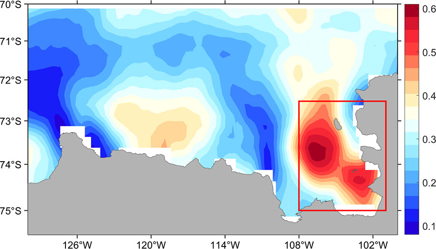
Figure 2 Annual standard deviation for SST in January after a 2–8 year Butterworth bandpass filter. The red rectangle represents the study area within Pine Island Bay, bound by 72.5°S–75°S and 101°W–108°W.
We therefore selected the PIB region (i.e., the red rectangle at 72.5°S–75°S, 101°W–108°W shown in Figure 2) as the key area from which to analyze the interannual variability of SST in January. The regional averaged SST anomaly (SSTa) in the PIB shows significant interannual variability between 1982 and 2022 (Figure 3). Before 1990 and after 2004, SSTa is relatively stable, with the exception of 2012 and 2014. Notably, SSTa between 1990 and 2004 exhibits significant fluctuations. To better investigate SSTa variation, we defined two types of years: warmer years (SSTa > +1 stdv) and cooler years (SSTa < −1 stdv) (Jacobs and Comiso, 1989; Free et al., 2005); thus, five warmer years (1992, 1997, 2002, 2003, and 2014) and seven cooler years (1990, 1994, 1998, 2000, 2001, 2004, and 2012) were selected (Supplementary Figure S2).
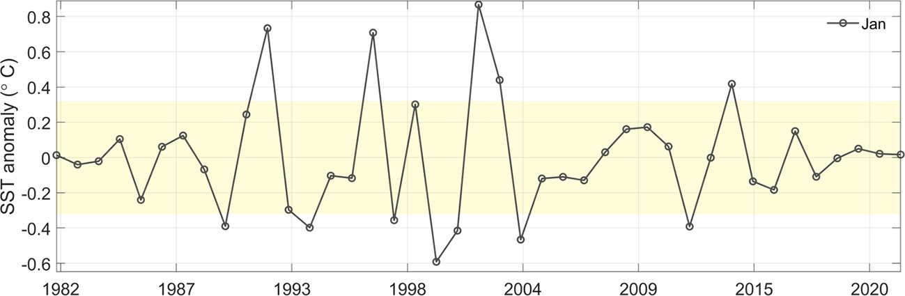
Figure 3 Time series for sea surface temperature anomaly (SSTa) in January averaged over the study area. The range of ±1 standard deviation is shaded in yellow.
SST in anomalous years
By conducting a composite analysis of SST in warmer and cooler years, it is clear that SST in warmer years is generally higher than that in cooler years throughout the whole AS, especially in the PIB. In warmer years, PIB is the warmest region, with SST up to 0.7° (Figure 4A) and a regional averaged SST of almost 0°. Unlike warmer years, sea ice still covers the AS during cooler years, and the ASP is the warmest region. The highest SST at PIB is lower than 0°, and the regional averaged SST can drop as low as −1.1° (Figure 4B).
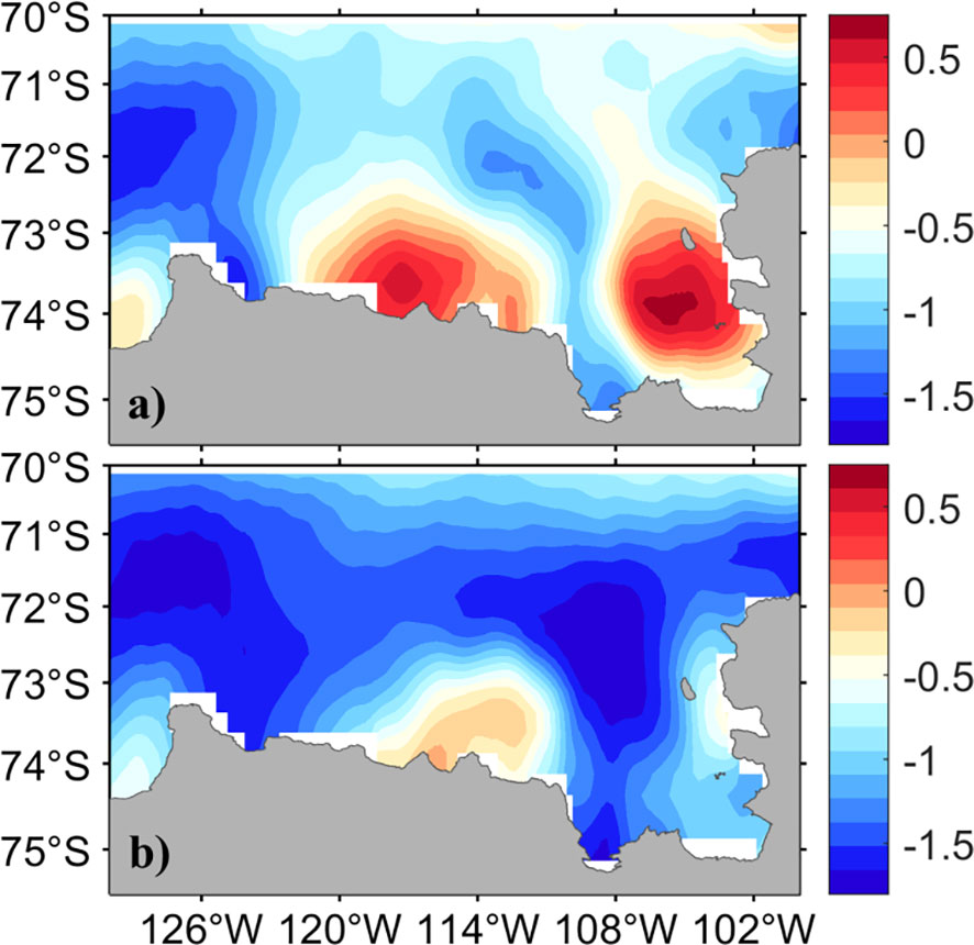
Figure 4 Distribution of sea surface temperature during (A) warmer years and (B) cooler years.
Atmospheric forcing and sea ice concentration in anomalous years
Similar composite analysis was used to address atmospheric forcing in January of warmer/cooler years (Figure 5). The 10 m wind is stronger near the shore than in the open sea, with the largest speeds exceeding 10 m/s in both warmer and cooler years. T2m in January of the AS is very cold; indeed, the maximum T2m at PIB reaches values as low as −1.1° (−1.4°) in warmer (cooler) years, with the regional mean T2m of −2.2° (−2.7°); thus, T2m in January is almost 2° cooler than SST, which is confirmed by the heat flux illustrated in Figure 6. Unlike in cooler years, the AS winds show an eastern anomaly of approximately 2 m/s in warmer years. Simultaneously, T2m of the AS is warmer (maximum: +1.7°) south of 73°S and cooler (maximum: −0.2°) north of 73°S. T2m at PIB in warmer years is at most 1.2° warmer than in cooler years, and the regional averaged is 0.6° warmer (Figure 5C).
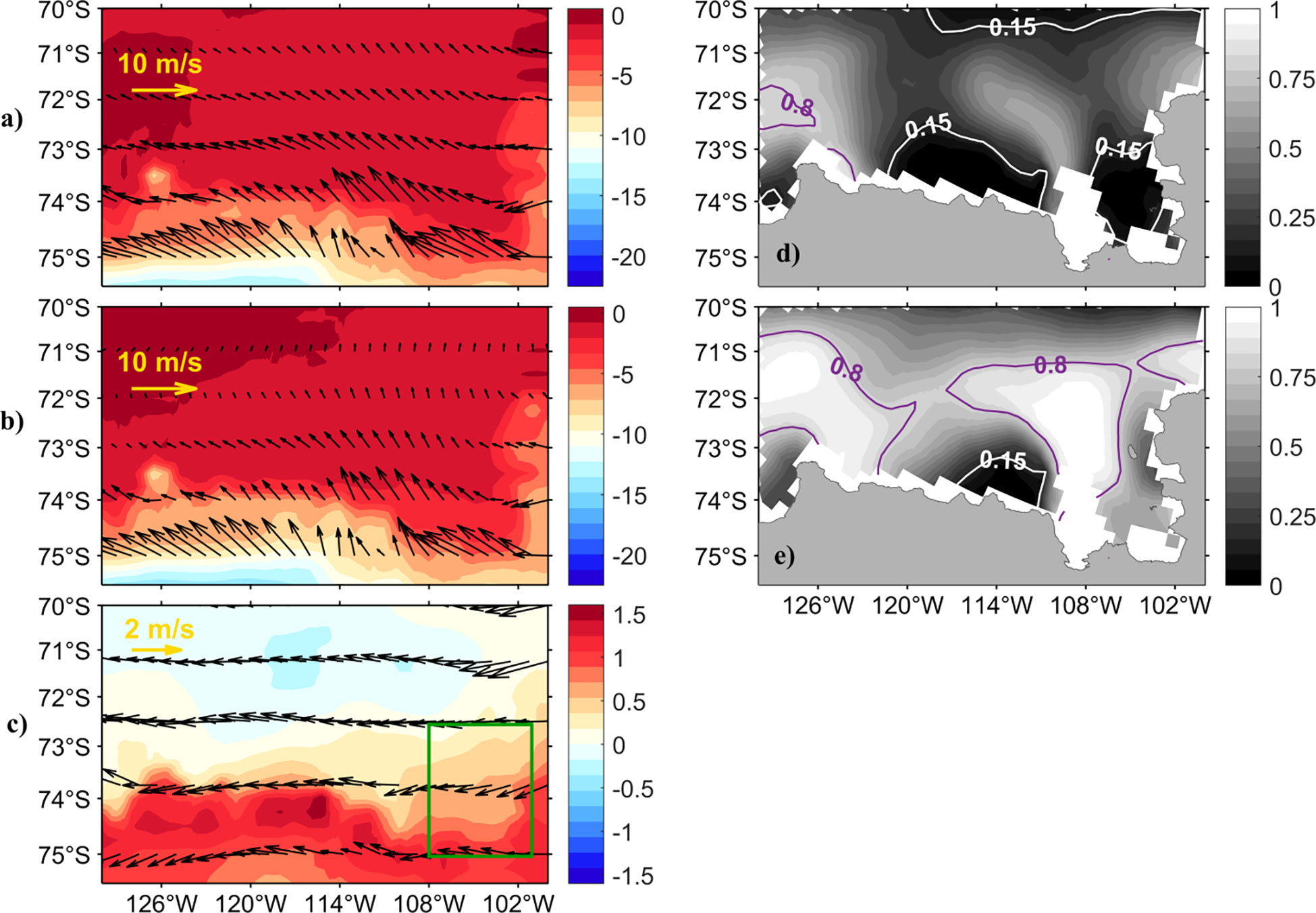
Figure 5 Distribution of air temperature (T2m, color shading) and 10 m wind (vector) during (A) warmer years and (B) cooler years. (C) Differences between 10 m wind and T2m for warmer and cooler years. The distributions of sea ice concentration (SIC, color shading) in warmer and cooler years are shown as (D) and (E), respectively. 15% SIC is marked by white lines and 80% SIC is marked by purple lines. The study area within the PIB is marked with a green rectangle in (C).
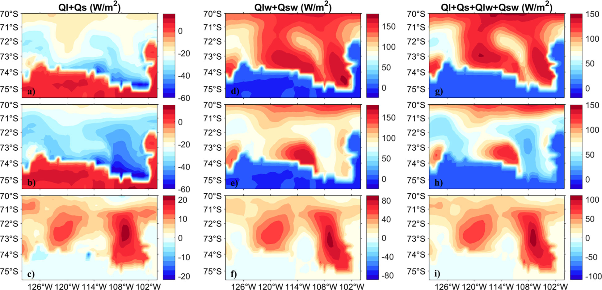
Figure 6 The first column shows the sum of the surface latent and sensible heat flux for (A) warmer years, (B) cooler years, and (C) the difference between them. The second column shows the sum of the surface net solar and thermal radiation for (D) warmer years, (E) cooler years, and (F) the difference between them. The third column shows the total net heat flux for (G) warmer years, (H) cooler years, and (I) the difference between them. Vertical heat fluxes are positive downwards.
Due to the cooler T2m above PIB, the ocean loses heat flux (Ql + Qs) to air during both warmer and cooler years, undergoing a greater loss by 24 W/m2 in cooler years (Figure 6C). In terms of total surface radiation (Qw; Qlw + Qsw), in warmer (cooler) years, the maximum Qw at PIB is 161 W/m2 (116 W/m2), and the regional mean value is 161 W/m2 (75 W/m2) (Figures 6D, E), i.e., there is a difference of 86 W/m2 between warmer and cooler years, in which Qsw contributes the most, approximately 83 W/m2 (not shown). Therefore, the net surface heat flux (QT; Ql + Qs + Qlw + Qsw) at PIB in warmer years is 110 W/m2 more than that in cooler years (Figure 6I), in which Qw contributes approximately 80%. Downward Qsw is primarily affected by greenhouse gases, aerosols, and albedo (e.g., Mitra, 1996), and areas covered by ice have high albedos. We consider that the large difference of Qsw between warmer and cooler years could be verified by SIC, as shown in Figures 5D, E. During warmer years, the regional mean SIC at PIB is lower than 15% but more than 68% in cooler years. High SIC (high albedo) in cooler years prevents the downward radiation, and vice versa.
Correlations of SSTa with QT and SIC
Using composite analysis, we find that QT and SIC are significantly different in warmer and cooler years, motivating us to consider whether they are related to interannual variations in SST. As shown in Figure 7, there is a remarkable positive correlation between SSTa and QT (correlation coefficient up to 0.72; Figure 7A). Due to the high albedo of sea ice, QT is strongly inversely associated with SIC, having a negative correlation coefficient of −0.88 (Figure 7B). Unsurprisingly, a strong negative correlation exists between SSTa and SIC (correlation coefficient −0.75; Figure 7C), that is, areas covered by low (high) SIC will absorb more (less) downward radiation, resulting in warmer (cooler) SSTs. Note that the coefficient values above are all significant at the 95% confidence level.
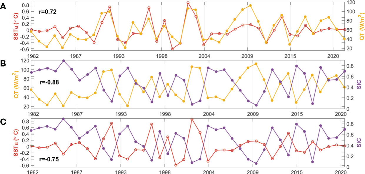
Figure 7 Time series of (A) sea surface temperature anomaly (SSTa) and surface net heat flux (QT). (B) QT and sea ice concentration (SIC). (C) SSTa and SIC. The correlation coefficients of each two variables in each panel are indicated.
In order to shed light on the mechanism of interannual variation in SST, it is necessary to determine why SIC changes. Variations of SIC are subject to multiscale ocean dynamics and air–sea interactions, such as ocean currents, wind-associated sea ice motion, and the advection of freshwater and heat (Weeks, 2010; Hobbs et al., 2016). In addition, large-scale atmospheric oscillations, such as the Southern Annular Mode (SAM), the El-Niño Southern Oscillation (ENSO), and the Amundsen Sea Low (ASL) have been found to influence underlying sea ice (Kohyama and Hartmann, 2016; Holland et al., 2018). In this paper, considering the available data, we primarily explore the influence of wind-associated sea ice motion on SIC. First, we define regional averaged SIC at PIB as an index, and then calculate its correlation with sea ice motion in October (Figures 8A, B) and November (Figures 8C, D). No significant correlations were observed between sea ice motion in December/January and SIC at the 95% confidence level (not shown). Although sea ice motion data is insufficient at PIB, it still shows a clear negative correlation with SIC. As shown in Figure 8D, SIC at PIB shows a strong inverse association with northward sea ice motion in November, having a maximum negative correlation coefficient of −0.82. In addition to sea ice motion at PIB, SIC also shows a strong relationship with sea ice motion north of PIB, with maximum correlation coefficients of −0.53 and −0.70 in October and November, respectively. In November, the northward sea ice motion at PIB and north of PIB both play an important role in SIC variation during the following January.
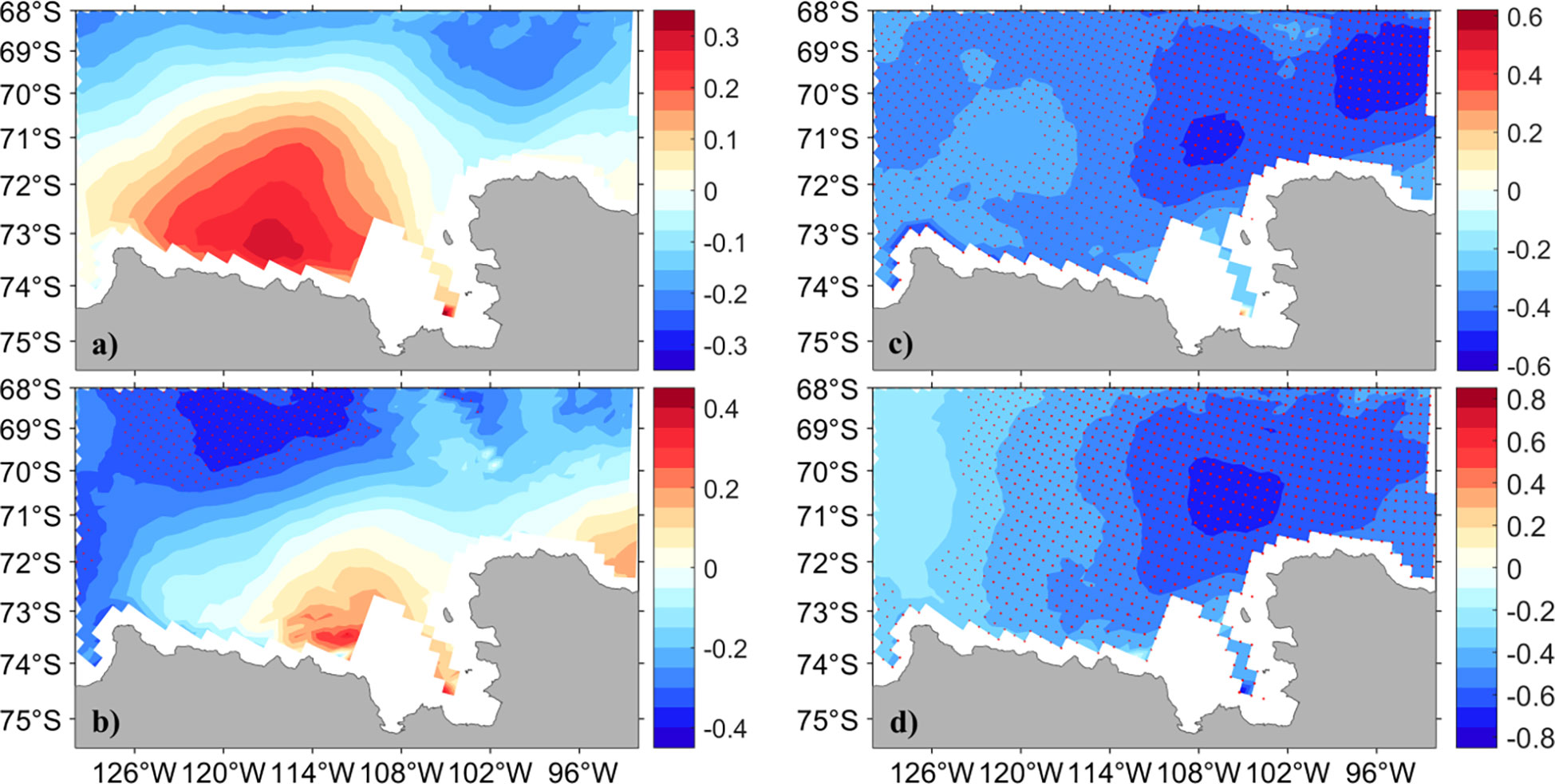
Figure 8 Distribution of the correlation coefficient between SIC in January and eastward/northward sea ice motion in October (A/B) and November (C/D) of the previous year. Red dots indicate significant correlations at the 95% confidence level.
Case studies of 1997 (warmer) and 1998 (cooler)
To more comprehensively explore the evolution of SST, we considered the warmer 1997 (Figure 9) and cooler 1998 (Figure 10) as individual case studies to examine in detail. During 1997, PIB was the warmest in the AS, with maximum SST exceeding 1° and regional mean SST above 0° (Figure 9A); during this time, SIC was as low as 12%. In January of 1998, the maximum SST at PIB was only 0.6°, and the regional mean SST was as low as −1°, with SIC at PIB as high as 66%. Given the strong inverse relationship between SIC and sea ice motion, and since sea ice motion is mainly driven by wind, we considered 10 m wind and SLP in November of the previous warmer and cooler years in order to better understand sea ice motion.
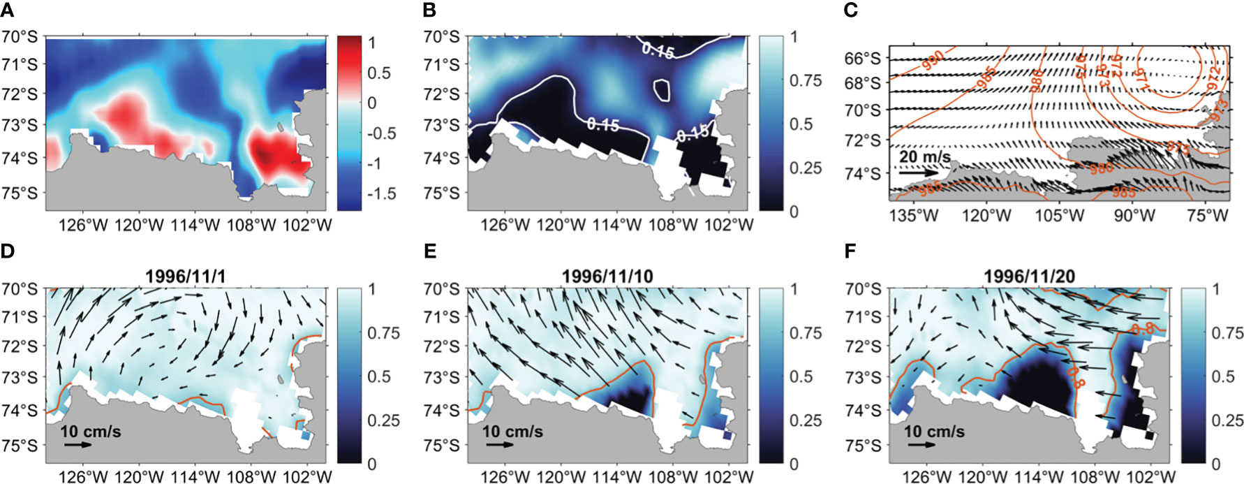
Figure 9 Spatial distributions of (A) mean sea surface temperature and (B) mean sea ice concentration during January of the warmer year 1997. (C) Mean 10 m wind in November 1996, including mean sea level pressure (tan contours). Spatial distributions of daily sea ice concentration (color shading) and motion (vectors) are shown in (D), (E), and (F), respectively. 15% and 80% SIC contours are marked by white and tan lines, respectively.
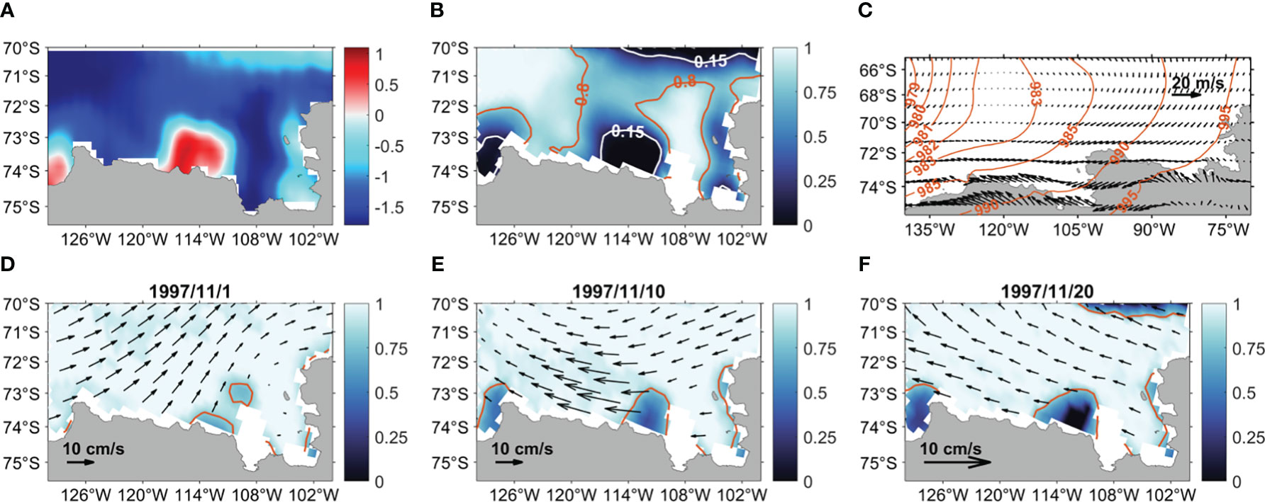
Figure 10 As Figure 9, but for the cooler year 1998.
As shown in Figure 9C, the low center of SLP in November was located northeast of the AS; thus, southeast wind existed at PIB, with the maximum (regional mean) wind speed exceeding 8 (5) m/s, and V10 reaching 5 m/s, with a regional mean speed of 3 m/s. On November 1, the whole AS was covered by sea ice, with SIC exceeding 91%, and sea ice moving clockwise (Figure 9D). Later, on November 10, the ASP became slightly exposed, and SIC at PIB began to decrease, with the regional mean (minimum) SIC of 75% (24%). Driven by the southeast wind, sea ice moved northwest, away from the coast, with a maximum velocity of approximately 20 cm/s. By November 20, the area of SIC below 80% increased in size, including both PIB and ASP. The regional averaged SIC at PIB decreased as low as 38%, and there was even no ice covered near the coast.
In the November before the cooler 1998, however, the low center of the SLP was located northwest of AS, and the 10 m wind was almost eastward south of 72°S, with little southward component. The maximum (regional mean) wind speed was almost 8 (4) m/s, with a maximum (regional mean) V10 of 3 (−0.6) m/s. On November 1, 1997, sea ice moved northeast, and SIC in AS was more than 93% (Figure 10D), i.e., almost the same as that in Figure 9D. Later, on November 10, SIC at PIB was still approximately 90%. The sea ice moved almost westward, consistent with the almost eastward wind speed (Figure 10C), and its velocity decreased gradually from near-shore to open sea. Subsequently, the distribution of SIC at PIB on November 20 was almost the same as that on November 10; the sea ice continued to move westward, but with a lower speed of approximately 5 cm/s.
Discussion
In this study, we find SST at PIB of the AS shows significant interannual variability, and then investigate its reason by using composite analysis and correlation analysis. The results show that SST variation is mainly affected by the atmosphere, that is, wind-driven sea ice motion directly affect SIC (r=-0.82), and SIC is highly correlated with the radiation flux (r=-0.88), especially the solar flux due to its high albedo. Further, how to understand the wind variation and what is the influence of ocean on SST?
Firstly, the wind itself is likely triggered by the unsteady ASL in the AS, especially the ASL’s locations. As shown in Figure 11, the composite location of ASL occurs to the northeast of the AS in the November before warmer years (Figure 11A), and northwest of the AS in the November before the cooler years (Figure 11B), between which a southwest wind anomaly of approximately 5 m/s exists (Figure 11C). The changes of ASL’s locations cause different wind patterns, with its corresponding influence illustrated in Figures 9 and Figure 10. In November 1996 (1997), the center of ASL was located on northeast (northwest) of the AS, thus, V10 at PIB exceeded 5 m/s (3 m/s), with a regional mean V10 as high as 3 m/s (−0.6 m/s in the opposite direction); this caused northwest (almost westward) sea ice movement away from the coast, which resulted in a regional mean SIC as low as 12% (as high as 66%). Future studies should note that variations of SIC and ASL result from interactions between many dynamic processes. Many studies have identified that ENSO and SAM are associated with ASL (Goyal et al., 2021; Maclennan and Lenaerts, 2021); however, these issues are beyond the scope of this paper.
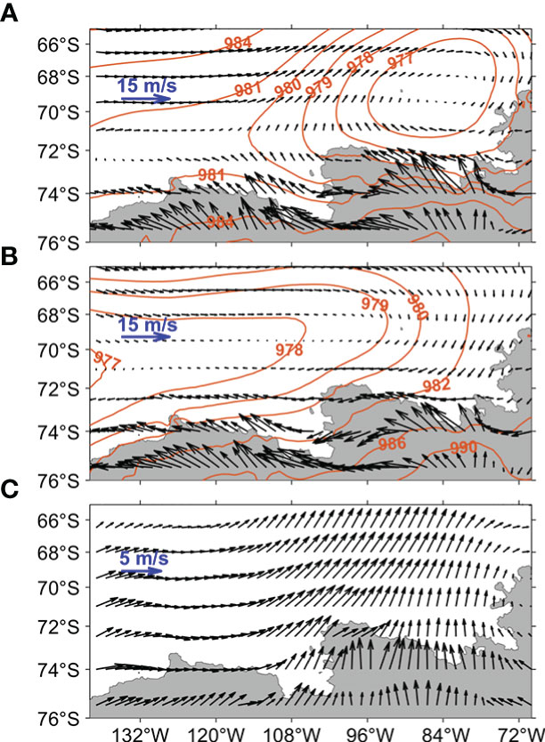
Figure 11 Distribution of the 10 m wind (vector) and mean sea level pressure (tan contours) in November before (A) warmer years and (B) cooler years. (C) Difference between (A) and (B).
Secondly, how to evaluate the influence of ocean on SST? Recent studies suggested that the melting of WAIS was mainly controlled by the ocean, that is, the enhanced warm Circumpolar Deep Water (CDW) driven by the eastward wind anomalies (e.g., Holland et al., 2019; Naughten et al., 2022). Whether this warm CDW will affect the surface temperature? Based on the model results, Naughten et al. (2022) analyzed the heat budget terms at 106°W (Thwaites Ice Shelf) and pointed out that the influence of the warm CDW is mainly concentrated at mid-depth with the range of 200 to 500 m. In addition, as Figure 3 in Naughten et al. (2022) showed, both 3D advection and shortwave radiation played important roles on the heat budget near-surface. In this study, radiation flux is proved to be highly correlated with SST variation, thus, to evaluate the effects of ocean, we should use model in the future work to investigate the subsurface upwelling (downwelling) due to off-coast (into-coast) winds of the AS.
Conclusions
Over recent decades, major changes have happened in the AS, including significant warming and ice shelf melting (e.g., Bromwich et al., 2013; Naughten et al., 2022; Zhang et al., 2019). Recent research has indicated a significant warming trend in AS SST, but interannual variations have not been studied in detail.
Based on the 41-year (1982–2022) OISST dataset, we find that SST in the PIB (72.5°S–75°S, 101°W–108°W) of the AS exhibits the largest fluctuations, with stdv values up to 0.6° (Figure 2) and regional mean SSTa showing significant interannual variability (Figure 3). Thereafter, five warmer years (1992, 1997, 2002, 2003, and 2014) and seven cooler years (1990, 1994, 1998, 2000, 2001, 2004, and 2012) were selected to represent instances in which SSTa was outside ±1 stdv. Composite analysis was conducted using SST and atmospheric forcing in January, and the results indicate that, for warmer years, the warmest SST at PIB could reach 0.7°, with a regional averaged SST of almost 0°; for cooler years, the highest SST at PIB was lower than 0°, and the regional averaged SST dropped as low as −1.1°. The maximum (regional mean) T2m was approximately −1.1° (−2.2°) in warmer years and approximately −1.4° (−2.7°) in cooler years (Figures 5A, B). In terms of surface heat exchange, warmer years contribute 110 W/m2 more QT than cooler years (Figure 6F), in which total surface radiation (Qlw + Qsw) accounted for almost 80%. This difference in heat flux is assumed to be consistent with SIC at PIB, which is lower than 15% (more than 68%) in warmer (cooler) years (Figures 5D, E).
Correlation analysis suggests that QT in the PIB is related to SSTa, with a correlation coefficient up to 0.72 (Figure 7A). Influenced by the high albedo of sea ice, QT shows a strongly inverse association with SIC, having a correlation coefficient of −0.88 (Figure 7B). Thus, a strong negative correlation exists between SIC and SSTa, with the correlation coefficient of −0.75 (Figure 7C). When SIC is high (low), its high (low) albedo causes the ocean to absorb less (more) QT; this ultimately results in a lower (higher) SST; as such, SIC is probably the “culprit” behind the warmer and cooler SSTs observed at PIB. Further analysis suggests that the SIC variation is associated with previous sea ice motion, and specifically, the northward sea ice motion in November can explain approximately 82% of SIC variations in the following January (Figure 8), which is driven by the ASL-associated wind variations as shown in Figure 11.
Therefore, the possible mechanism of interannual SST variation in the AS is summarized as follows. In the previous November, influenced by the northeast (northwest) location of ASL above the AS, a northwest (westward) wind prevails. This causes sea ice to be pushed off (into) the coast, resulting in a decrease (increase) of SIC. Subsequently, the solar radiation heat flux increases (decreases) due to absent (rich) ice, together with subsurface upwelling (downwelling) due to off-coast (into-coast) winds, and SST increases (decreases) during the following January.
In this paper, we explored the interannual variability of SST during the austral summer of the AS, and determined its possible mechanism. In future work, we should link the ASL with the large-scale atmospheric oscillations (ENSO and SAM) to better explain the SST variation in the AS, and also should use model to evaluate the specific influence of ocean on SST.
Data availability statement
The original contributions presented in the study are included in the article/Supplementary Material. Further inquiries can be directed to the corresponding author.
Author contributions
LY: investigation, data analysis and writing. HH&Hailong Liu: supervision, revision and project administration. Hengling Leng&PL: providing suggestions and editing. All authors contributed to the article and approved the submitted version.
Funding
This study is supported by Impact and Response of Antarctic Seas to Climate Change Program (01-01-01B, 02-01-02), the Project of State Key Laboratory of Satellite Ocean Environment Dynamics, Second Institute of Oceanography (No. SOEDZZ2206), Science and Technology Program of Guangzhou, China, (202002030492), and the Natural Science Foundation of Guangdong Province, China (2022A1515011967).
Conflict of interest
The authors declare that the research was conducted in the absence of any commercial or financial relationships that could be construed as a potential conflict of interest.
Publisher’s note
All claims expressed in this article are solely those of the authors and do not necessarily represent those of their affiliated organizations, or those of the publisher, the editors and the reviewers. Any product that may be evaluated in this article, or claim that may be made by its manufacturer, is not guaranteed or endorsed by the publisher.
Supplementary material
The Supplementary Material for this article can be found online at: https://www.frontiersin.org/articles/10.3389/fmars.2023.1050955/full#supplementary-material
References
Arrigo K. R., Lowry K. E., van Dijken G. L. (2012). Annual changes in sea ice and phytoplankton in polynyas of the amundsen Sea, Antarctica. Deep Sea Res. Part II: Topical Stud. Oceanogr. 71, 5–15. doi: 10.1016/j.dsr2.2012.03.006
Arrigo K. R., Van Dijken G. L. (2003). Phytoplankton dynamics within 37 Antarctic coastal polynya systems. J. Geophys. Res.: Oceans 108 (C8), 3271. doi: 10.1029/2002JC001739
Arrigo K. R., van Dijken G. L., Strong A. L. (2015). Environmental controls of marine productivity hot spots around Antarctica. J. Geophys. Res. Oceans. 120 (8), 5545–5565. doi: 10.1002/2015JC010888
Banzon V., Smith T. M., Chin T. M., Liu C., Hankins W. (2016). A long-term record of blended satellite and in situ sea-surface temperature for climate monitoring, modeling and environmental studies. Earth Syst. Sci. 8, 165–176. doi: 10.5194/essd-8-165-2016
Bromwich D. H., Nicolas J. P., Monaghan A. J., Lazzara M. A., Keller L. M., Weidner G. A., et al. (2013). Central West Antarctica among the most rapidly warming regions on earth. Nat. Geosci. 6 (2), 139–145. doi: 10.1038/ngeo1671
Comiso J. C. (2000). Variability and trends in Antarctic surface temperatures from in situ and satellite infrared measurements. J. Climate 13 (10), 1674–1696. doi: 10.1175/1520-0442(2000)013<1674:VATIAS>2.0.CO;2
Eayrs C., Li X., Raphael M. N., Holland D. M. (2021). Rapid decline in Antarctic sea ice in recent years hints at future change. Nat. Geosci. 14 (7), 460–464. doi: 10.1038/s41561-021-00768-3
Free M., Seidel D. J., Angell J. K., Lanzante J., Durre I., Peterson T. C. (2005). Radiosonde atmospheric temperature products for assessing climate (RATPAC): A new data set of large-area anomaly time series. J. Geophys. Res.: Atmospheres 110 (D22), D22101. doi: 10.1029/2005JD006169
Garcia-Eidell C., Comiso J. C., Berkelhammer M., Stock L. (2021). Interrelationships of sea surface salinity, chlorophyll-α concentration, and sea surface temperature near the Antarctic ice edge. J. Climate 34 (15), 6069–6086. doi: 10.1175/JCLI-D-20-0716.1
Good S., Fiedler E., Mao C., Martin M. J., Maycock A., Reid R., et al. (2020). The current configuration of the OSTIA system for operational production of foundation sea surface temperature and ice concentration analyses. Remote Sens. 12 (4), 720. doi: 10.3390/rs12040720
Goyal R., Jucker M., Gupta A. S., Hendon H., England M. (2021). Zonal wave 3 pattern in the southern hemisphere generated by tropical convection. Nature Geoscience 14(10), 732–738. doi: 10.21203/rs.3.rs-320008/v1
Hersbach H., Bell B., Berrisford P., Biavati G., Horányi A., Muñoz Sabater J., et al. (2019). ERA5 monthly averaged data on single levels from 1959 to present (Copernicus Climate Change Service (C3S) Climate Data Store (CDS), 10, 252–266. doi: 10.24381/cds.f17050d7
Hirahara S., Ishii M., Fukuda Y. (2014). Centennial-scale sea surface temperature analysis and its uncertainty. J. Climate 27 (1), 57–75. doi: 10.1175/JCLI-D-12-00837.1
Hobbs W. R., Bindoff N. L., Raphael M. N. (2015). New perspectives on observed and simulated Antarctic sea ice extent trends using optimal fingerprinting techniques. J. Climate 28 (4), 1543–1560. doi: 10.1175/JCLI-D-14-00367.1
Hobbs W. R., Massom R., Stammerjohn S., Reid P., Williams G., Meier W. (2016). A review of recent changes in southern ocean sea ice, their drivers and forcings. Global Planetary Change 143, 228–250. doi: 10.1016/j.gloplacha.2016.06.008
Holland M. M., Landrum L., Raphael M. N., Kwok R. (2018). The regional, seasonal, and lagged influence of the amundsen sea low on Antarctic sea ice. Geophys. Res. Lett. 45 (11), 227–311. doi: 10.1029/2018GL080140
Holland P. R., Bracegirdle T. J., Dutrieux P., Jenkins A., Steig E. J. (2019). West Antarctic ice loss influenced by internal climate variability and anthropogenic forcing. Nature Geoscience, 12(9), 718–724.
Huang B., Thorne P. W., Banzon V. F., Boyer T., Chepurin G., Lawrimore J. H., et al. (2017). NOAA Extended reconstructed sea surface temperature (ERSST), version 5. NOAA Natl. Centers Environ. Inf. 30 (8179-8205), 25. doi: 10.1175/JCLI-D-16-0836.1
Jacobs S. S., Comiso J. C. (1989). Sea Ice and oceanic processes on the Ross Sea continental shelf. J. Geophys. Res.: Oceans 94 (C12), 18195–18211. doi: 10.1029/JC094iC12p18195
Key J. R., Collins J. B., Fowler C., Stone R. S. (1997). High-latitude surface temperature estimates from thermal satellite data. Remote Sens. Environ. 61 (2), 302–309. doi: 10.1016/S0034-4257(97)89497-7
King J. C., Marshall G. J., Colwell S., Arndt S., Allen-Sader C., Phillips T. (2022). The performance of the ERA-interim and ERA5 atmospheric reanalyses over weddell Sea pack ice. J. Geophys. Res.: Oceans 127, e2022JC018805. doi: 10.1029/2022JC018805
Kohyama T., Hartmann D. L. (2016). Antarctic Sea ice response to weather and climate modes of variability*. J. Climate 29, 721–741. doi: 10.1075/jcli-d-15-0301.110.1175/jcli-d-15-0301.1
Lebedev S. A. (2007). Interannual trends in the southern ocean sea surface temperature and sea level from remote sensing data. Russian J. Earth Sci. 9 (3), 1–6. doi: 10.2205/2007ES000283
Lhardy F., Bouttes N., Roche D. M., Crosta X., Waelbroeck C., Paillard D. (2021). Impact of southern ocean surface conditions on deep ocean circulation during the LGM: a model analysis. Climate Past 17 (3), 1139–1159. doi: 10.5194/cp-17-1139-2021
Maclennan M. L., Lenaerts J. T. (2021). Large-Scale atmospheric drivers of snowfall over thwaites glacier, Antarctica. Geophys. Res. Lett. 48 (17), e2021GL093644. doi: 10.1029/2021GL093644
Maheshwari M., Singh R. K., Oza S. R., Kumar R. (2013). An investigation of the southern ocean surface temperature variability using long-term optimum interpolation SST data. ISRN Oceanography 2013, 1–9.
Meier W. N., Fetterer F., Windnagel A. K., Stewart. J. S. (2021) NOAA/NSIDC climate data record of passive microwave Sea ice concentration, version 4 [Data set] (Boulder, Colorado USA: National Snow and Ice Data Center) (Accessed 09-05-2022).
Mitra A. P. (1996). Global change greenhouse gas emission in India-methane budget estimates from rice fields based on data available up to 1995. Scientific report no. 10. New Delhi, India: Publication and Information Directorate, CSIR.
Morlighem M., Rignot E., Binder T., Blankenship D. D., Drews R., Eagles G., et al. (2020). Deep glacial troughs and stabilizing ridges unveiled beneath the margins of the Antarctic ice sheet. Nat. Geosci. 13, 132–137. doi: 10.1038/s41561-019-0510-8
Nagy H., Elgindy A., Pinardi N., Zavatarelli M., Oddo P. (2017). A nested pre-operational model for the Egyptian shelf zone: Model configuration and validation/calibration. Dynamics Atmospheres Oceans 80, 75–96. doi: 10.1016/j.dynatmoce.2017.10.003
Nagy H., Lyons K., Nolan G., Cure M., Dabrowski T. (2020). A regional operational model for the north East Atlantic: Model configuration and validation. J. Mar. Sci. Eng. 8 (9), 673. doi: 10.3390/jmse8090673
Naughten K. A., Holland P. R., Dutrieux P., Kimura S., Bett D. T., Jenkins A. (2022). Simulated twentieth-century ocean warming in the amundsen Sea, West Antarctica. Geophys. Res. Lett. 49 (5), e2021GL094566. doi: 10.1029/2021GL094566
Oza S. R., Singh R. K. K., Srivastava A., Dash M. K., Das I. M. L., Vyas N. K. (2011). Inter-annual variations observed in spring and summer Antarctic sea ice extent in recent decade. Mausam 62 (4), 633–640. doi: 10.54302/mausam.v62i4.381
Paolo F. S., Fricker H. A., Padman L. (2015). Volume loss from Antarctic ice shelves is accelerating. Science 348, 327–331. doi: 10.1126/science.aaa0940
Parkinson C. L. (2019). A 40-y record reveals gradual Antarctic sea ice increases followed by decreases at rates far exceeding the rates seen in the Arctic. Proceedings of the National Academy of Sciences. 116 (29), 14414–14423.
Parkinson C. L., Cavalieri D. J. (2012). Antarctic Sea ice variability and trends 1979–2010. Cryosphere 6 (4), 871–880. doi: 10.5194/tc-6-871-2012
Payne A. J., Vieli A., Shepherd A. P., Wingham D. J., Rignot E. (2004). Recent dramatic thinning of largest West Antarctic ice stream triggered by oceans. Geophys. Res. Lett. 31, L23401. doi: 10.1029/2004GL021284
Pritchard H., Ligtenberg S. R., Fricker H. A., Vaughan D. G., van den Broeke M. R., Padman L. (2012). Antarctic Ice-sheet loss driven by basal melting of ice shelves. Nature 484 (7395), 502–505. doi: 10.1038/nature10968
Purich A., England M. H., Cai W., Sullivan A., Durack P. J. (2018). Impacts of broad-scale surface freshening of the southern ocean in a coupled climate model. J. Climate 31 (7), 2613–2632. doi: 10.1175/JCLI-D-17-0092.1
Rayner N. A. A., Parker D. E., Horton E. B., Folland C. K., Alexander L. V., Rowell D. P., et al. (2003). Global analyses of sea surface temperature, sea ice, and night marine air temperature since the late nineteenth century. J. Geophys. Res.: Atmospheres 108 (D14), 4407. doi: 10.1029/2002JD002670
Rignot E., Mouginot J., Scheuchl B., van den Broeke M., van Wessem M. J., Morlighem M. (2019). Four decades of Antarctic ice sheet mass balance from 1979-2017. Proceedings of the National Academy of Sciences of the United States of America. 116 (4), 1095–1103.
Tschudi M., Meier W. N., Stewart J. S., Fowler C., Maslanik. J. (2019) Polar pathfinder daily 25 km EASE-grid Sea ice motion vectors, version 4 [Data set] (Boulder, Colorado USA: NASA National Snow and Ice Data Center Distributed Active Archive Center) (Accessed 09-05-2022).
Keywords: Amundsen Sea, summer sea surface temperature, interannual variability, Pine Island Bay, sea ice concentration, Amundsen Sea low-associated wind
Citation: Yu L-S, He H, Leng H, Liu H and Lin P (2023) Interannual variation of summer sea surface temperature in the Amundsen Sea, Antarctica. Front. Mar. Sci. 10:1050955. doi: 10.3389/fmars.2023.1050955
Received: 22 September 2022; Accepted: 06 March 2023;
Published: 20 March 2023.
Edited by:
Amelie Simon, University of Lisbon, PortugalCopyright © 2023 Yu, He, Leng, Liu and Lin. This is an open-access article distributed under the terms of the Creative Commons Attribution License (CC BY). The use, distribution or reproduction in other forums is permitted, provided the original author(s) and the copyright owner(s) are credited and that the original publication in this journal is cited, in accordance with accepted academic practice. No use, distribution or reproduction is permitted which does not comply with these terms.
*Correspondence: Hailun He, aGVoYWlsdW5Ac2lvLm9yZy5jbg==