- 1CNR – Consiglio Nazionale delle Ricerche, ISMAR – Istituto di Scienze Marine, Venice, Italy
- 2Department of Physical and Chemical Sciences, University of L’Aquila, L’Aquila, Italy
- 3Center of Excellence in Telesensing of Environment and Model Prediction of Severe Events (CETEMPS), University of L’Aquila, L’Aquila, Italy
- 4Climate Simulation and Prediction (CSP), Fondazione Centro Euro-Mediterraneo sui Cambiamenti Climatici (CMCC), Bologna, Italy
Due to their well-acknowledged capability in predicting habitat distributions, Habitat Suitability Models (HSMs) are particularly useful for investigating ecological patterns variations under climate change scenarios. The shallow coastal regions of the Northern Adriatic Sea, a sub-basin of the Mediterranean Sea, are studded with coralligenous outcrops recognized as important biodiversity hotspots exposed to the effects of climate change. In this research, we investigate the distributions of the Northern Adriatic Sea coralligenous habitats characterized by diverse species assemblages differently influenced by environmental factors, and provide a projection of how these might be impacted by climate change. Two models (Random Forest and MaxEnt), populated with occurrence data gathered from previous publications, environmental parameters’ from online databases (CMEMS, Bio-Oracle), and a set of dedicated ocean model simulations, are applied in recent past conditions and under a future severe climate change scenario (RCP 8.5). The model performance metrics confirm the ability of both approaches for predicting habitat distribution and their relationship with environmental conditions. The results show that salinity, temperature, and nitrate concentration are generally the most relevant variables in affecting the coralligenous outcrops distribution. The environmental variations projected under climate change conditions are expected to favour the spreading of opportunistic organisms, more tolerant to stressful conditions, at the expense of more vulnerable species. This will result in a shift in the distribution of these habitats, with a consequent potential loss of biodiversity in the Northern Adriatic Sea.
1 Introduction
Marine ecosystems play a key role in safeguarding the planet and in favoring human life. They host a large portion of the world’s biodiversity and provide many fundamental benefits to humans, delivering resources and supporting maritime activities, such as fishery, tourism and transportation, and representing a driver of the world economy (Freeman et al., 2013; Barbier, 2017). They do also play a central role in stabilizing the Earth’s climate system by contributing to buffer the effects of climate change on our planet (Melaku Canu et al., 2015). Nevertheless, the global climate change is deeply affecting oceanographic, biogeochemical, and hydrological processes that regulate the structure and functioning of marine systems (Leadley et al., 2014). In particular, starting from the 70s, abrupt shifts in current climate patterns (Cheung et al., 2009; Pereira et al., 2010; Cahill et al., 2012; Sloyan et al., 2016), alteration of frequency or intensity of environmental phenomena (Garcia-Reyes et al., 2015; Defforge and Merlis, 2017), increase in temperatures (IPCC, 2013b; Rhein et al., 2013) and ocean acidification (Hoegh-Guldberg et al., 2014) have been detected. These alterations lead to a higher probability and frequency of catastrophic events, mass mortality (IPCC, 2014; Pecl et al., 2017a; Pecl et al., 2017b), food webs alteration (Johnson et al., 2011), abrupt shifts in the seasonality of ecological processes (Deutsch et al., 2015; Lefort et al., 2015), and decline in ecosystem diversity and productivity (Short and Neckles, 1999; Behrenfeld et al., 2006; Hoegh-Guldberg et al., 2007; Polovina et al., 2008; Harley, 2011). As a cascade effect, shifts in marine organism populations, variations in species phenology, and interactions with serious impacts on ecosystem functioning have also been reported (Perry et al., 2005; Last et al., 2011; Doney et al., 2012).
The sensitivity of marine systems to climate change have been discussed in several Assessment Reports (hereby AR) of the Intergovernmental Panel on Climate Change (IPCC). Nevertheless, it was only since the fourth AR in 2007, that the impacts of climate change on marine ecosystems were addressed in deeper detail, with emphasis on the assessment of future ecosystems’ response and through a recognition of the complexity of these environments (Gissi et al., 2021; Fraschetti et al., 2022).
Because global warming has been pinpointed to be one of the main elements of climate change, and temperature is expected to keep rising in the upcoming decades, marine species will be forced to either adapt to the new conditions or find new suitable ecological niches (Lawler et al., 2006; Coll et al., 2012; Marras et al., 2015; García Molinos et al., 2016), with consequent shifts in habitat distributions.
Developed to predict the distribution of habitat in response to a given set of environmental factors, Habitat Suitability Models (hereafter HSMs) have been applied in an increasingly number of contexts, becoming important tools to support biodiversity management (Lawler et al., 2006; Degraer et al., 2008; Glockzin et al., 2009; Gogina and Zettler, 2010; Bates et al., 2013; Freeman et al., 2013; Guisan et al., 2013). In particular, HSMs can have an important role in ecosystem-based management planning (Guisan and Thuiller, 2005; Heikkinen et al., 2006; Pompe et al., 2008; Elith and Leathwick, 2009; Kharouba et al., 2009; Lavender et al., 2021), by helping in i) identifying priority areas of conservation (Cañadas et al., 2005), ii) assessing the spatial distribution of suitable habitats for a species or a community to live within protected areas (Monk et al., 2010), iii) predicting sites at risk of invasion by exotic species (Compton et al., 2010) and iv) investigating the distribution of possible diseases (Williams et al., 2010). These models can be grouped into two categories (Meineri et al., 2015): mechanistic methods aiming at reproducing the ecological dynamics by explicitly describing (and formalizing into equations to be solved by mean of numerical techniques) their driving processes (e.g. energy fluxes, biological interactions, dispersal); and correlative methods aiming instead at reproducing the distribution of species and habitats by addressing their probability of presence (or absence) under prescribed environmental parameters. By pursuing the emerging patterns instead of an explicit description of the ecological processes, the latter approach tends to be more efficient particularly in complex systems.
These tools are widely implemented in the Mediterranean Sea (Lauria et al., 2015; Giannoulaki et al., 2017), one of the worldwide biodiversity hotspots which has been predicted to be among the most impacted by global warming (Templado, 2014; Lionello and Scarascia, 2018) with many Mediterranean species at high risk of decline due to climate change (Vasilakopoulos et al., 2017). In particular, the growing and survival of calcifying organisms, such as corals and coralline algae, are threatened by the alteration of their optimal conditions (Freeman et al., 2013).
The coralligenous, a widespread habitat of the Mediterranean Sea, is recognized as a priority for conservation under the Habitats Directive (EU, 1992; 92/43/EEC) and the Marine Strategy Framework Directive (EU, 2008; 2008/56/EC) for its importance as a biodiversity hotspot (Gomes-Gras et al., 2019). It is the result of a balance between bioconstruction and bioeroding processes carried out by the associated organisms (Cerrano et al., 2001). These complex biogenic structures, characterized by holes and cavities, provide different microhabitats, microenvironments, and ecological gradients that host numerous species, especially coralline algae, mollusks, polychaetes, madrepores, and macroalgae (Ingrosso et al., 2018). Dim-light, narrow thermal oscillations and low water turbidity (influencing the filtering capacity of organisms) are among the main environmental conditions determining coralligenous growth and the number of associated species. The United Nations has identified this habitat as an ecosystem services provider (Action Plan for the protection of coralligenous and other calcareous bio-concretions in the Mediterranean Sea, 2017), and has remarked the need for its protection due to its vulnerability to climate change (Teixidó et al., 2013). At the European level, the EU Council (Regulation n°1967/2006) reported guidelines for sustainable fishery practices in the Mediterranean explicitly referring to the need to protect coralligenous habitat.
Coralligenous outcrops are scattered on the sandy-muddy seabed of the Northern Adriatic Sea (the northernmost region of the Mediterranean basin) and are locally known as tegnùe, trezze or grèbeni (Casellato and Stefanon, 2008). Differently from other bio-constructions, the tegnùe are observed to be associated with methane vents and hypothesized to be cemented by methane seeps mostly originating from microbial decomposition of fossil plant material, a characteristic that makes these outcrops unique in the Mediterranean Sea (Tosi et al., 2017 and references therein). Besides hosting highly diverse benthic communities, these outcrops play a fundamental role as reproductive and nursery areas and attract and protect numerous demersal and pelagic fish species, thus representing sites of high local interest for divers and fishermen (Cenci and Mazzoldi, 2006; Casellato et al., 2007).
This habitat is subject to conservation by two Natura 2000 (N2K) sites, namely the SPA/SAC IT3330009 “Trezze di San Pietro e Bardelli” and the SAC IT3250047 “Tegnùe di Chioggia”. The N2K network will likely expand in the Adriatic Sea to accomplish the conservation goals set up by global and European strategies - the Convention on Biological Diversity, the European Biodiversity Strategy 2030, the Global Sustainable Development Goals (de Francesco et al., 2020; Manea et al., 2021). As such, because of the potential effects of climatic change on this habitat, there is a need to implement durable conservation efforts in the area and guide the possible designation of new N2K sites for its protection.
In this direction, this study investigates the potential distribution of the coralligenous habitat in the Northern Adriatic Sea accounting for its species assemblages, and its possible shift under a future severe climate change scenario. Two methods of machine learning habitat suitability modelling are applied: Random Forest and Maximum Entropy (MaxEnt). Both of them are correlative approaches using the full spatial coverage of physical and biogeochemical variables to explore patterns of species distribution (Elith and Graham, 2009). They are both widely recognized as efficient tools for detecting and predicting habitat suitability distribution (Phillips et al., 2006; Thuiller and Münkemüller, 2010; Hijmans and Elith, 2013).
The study consists of two main modelling steps:
1. Habitat suitability analysis investigating the correlation between the distribution of different coralligenous habitat assemblages and the pattern of environmental variables (i.e. temperature, salinity, current velocity, light, nitrate, and phosphate concentration) during a historical period in the recent past (1999-2018, historical – “HIS” – run);
2. Habitat suitability analysis under future RCP 8.5 climate change scenario (2070-2099) and potential shift of the habitats assemblages by utilizing oceanic model simulations under the RCP 8.5 climate change scenario (Moss et al., 2010) (hereafter “SCE” run).
The results are discussed and interpreted in the light of the ecological properties of these systems and their implications for the coastal marine environment, aiming at providing usable information, alongside with some methodological remarks, for long-term planning, management and protection purposes.
2 Materials and methods
2.1 Analysis workflow overview
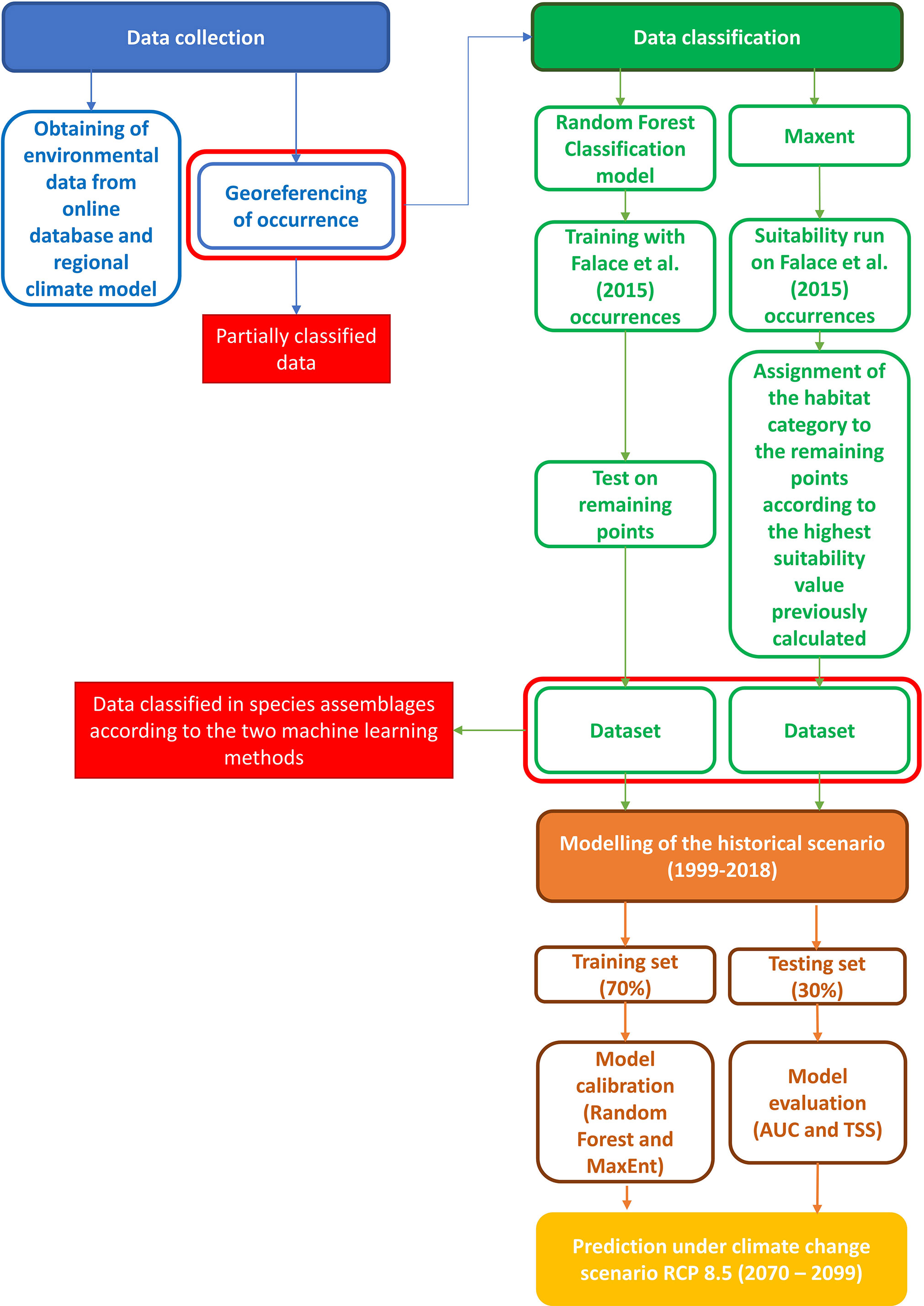
As a preparatory phase for the modelling activity, the collection of occurrence data was first carried out by georeferencing information obtained from the literature and partially classified under habitat assemblage categories. For those occurrences that were not classified in the literature, a classification phase was undertaken with a dedicated Random Forest and MaxEnt, using the occurrences already classified as a training dataset. This approach provided two distinct datasets (one for each method) with occurrences classified in habitat categories.
Subsequently, another set of Random Forest and MaxEnt based on the fully classified datasets was carried out for computing habitat suitability and its pattern under historical conditions. In this phase the datasets were split into training and test sets; the former was used to fit each of the HSMs on the available data and the latter was employed for the models skill assessment. The last modelling step addressed the prediction of coralligenous distribution under a climate change scenario. All data exploration, calculation, and model pre-processing were carried out using R software (R Development Core Team; version 4.0.5, https://www.r-project.org/), randomForest (version 4.6-14) (Liaw and Wiener, 2002) and dismo (version 1.3-3) (Hijmans et al., 2011) packages. The workflow of the investigation is reported in Figure 1.
2.2 Coralligenous occurrence data and habitat classification
Current coralligenous outcrops occurrences in the North Adriatic Sea were obtained by georeferencing (using ArcMap 10.2) the information contained in Falace et al. (2015) and Ponti et al. (2005) and combining them with the dataset compiled by Martin et al. (2014) in the framework of the projects MEDISEH and CoCoNET (Figure 2). In the study by Falace et al. (2015) the occurrences were clustered in three distinct habitat types (called A, B, and C) based on species compositions (a description of each habitat assemblage is reported in Table 1).
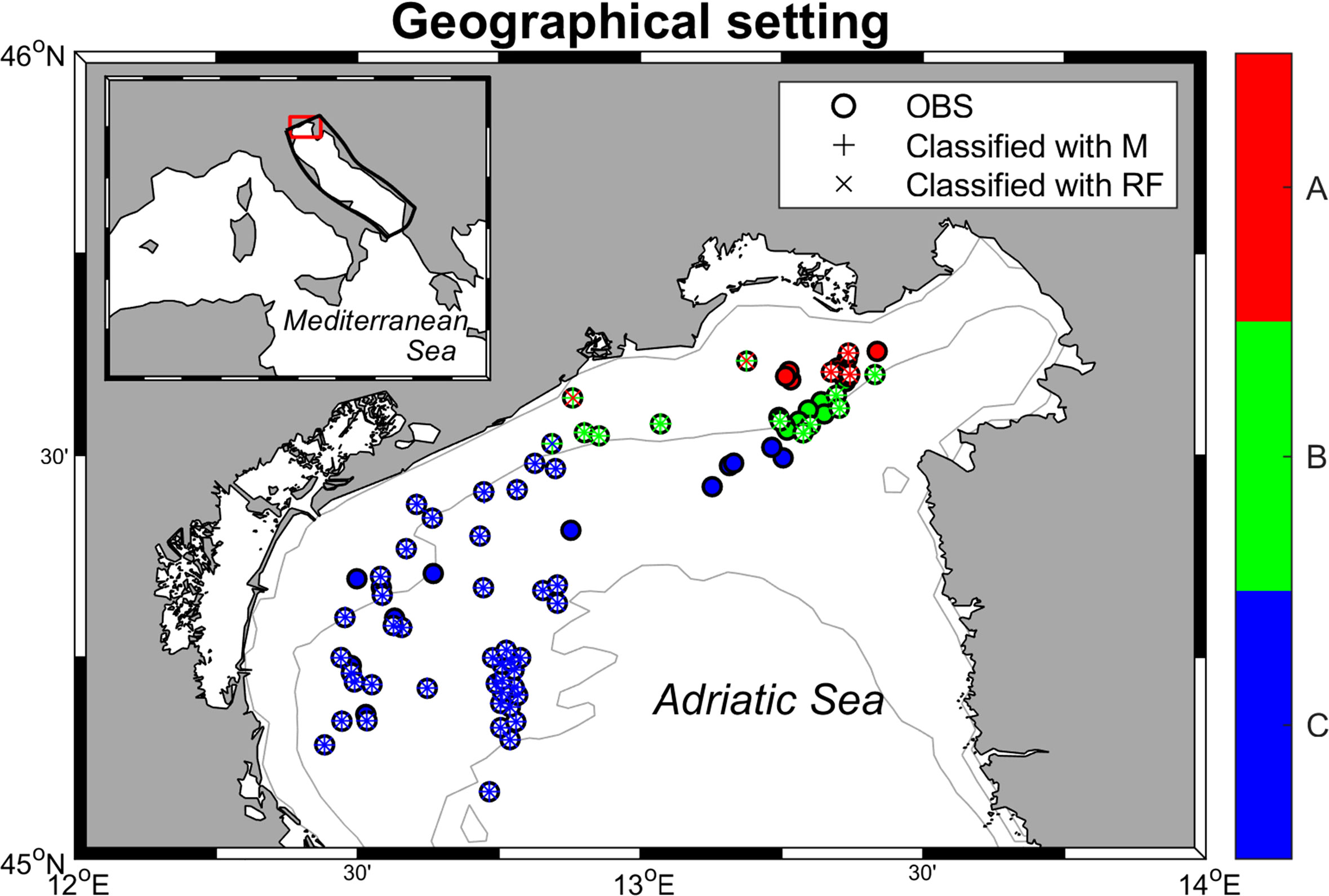
Figure 2 Geographical setting of the area of interest with the classified records according to the ML methods described in Paragraph 2.1. The filled ○ symbol means the occurrences already classified by Falace et al. (2015), while the unfilled ones represent occurrences from Ponti et al. (2005) and Martin et al. (2014). + symbol visualizes the records classified in the habitat typology with MaxEnt (M) and × stands for Random Forest (RF). Each color represents a habitat type.

Table 1 Habitat assemblages description extrapolated by Falace et al. (2015).
This habitat type classification was extended to all the coralligenous occurrences included in the present study to forecast the possible shift in communities’ composition. The habitat types were attributed by measuring, through the potential of HSMs, the correlation between environmental variables and species assemblages reported in Falace et al. (2015). Specifically, both algorithms were trained using the outcrop occurrences already categorized, while, the remaining points were used as a test set to which were then attributed a habitat category to each entry (workflow in Figure 1). Random Forest is widely used for the classification process through the implementation of categorical variables; while the application of MaxEnt for this purpose has required the assessment of the suitability of each habitat based on the already classified points and the classification of the uncategorized occurrences based on the highest suitability value.
2.3 Environmental variables
Several environmental variables were identified in the literature as particularly relevant in influencing coralligenous growth. In this study, temperature, salinity, current velocity, and light (all evaluated at the sea bottom) were considered, alongside with phosphate and nitrate concentrations averaged over the water column (Casellato and Stefanon, 2008; Martin et al., 2014; Falace et al., 2015). Near-bottom quantities for most of the variables were selected considering that the coralligenous outcrops are benthic habitats mainly composed of encrusting organisms. Only the values of nitrate and phosphate characterized the whole water column since these variables, adopted as proxies of nutrients, strongly influence the filter feeder organisms associated with the coralligenous (Piazzi et al., 2011; Gómez-Gras et al., 2021). Data were extracted from different sources Table 2. Simulated temperature, salinity, and current velocity at the sea bottom were provided by the numerical model ROMS (Regional Ocean Modeling System, Haidvogel et al., 2008) reproducing 3-D hydrodynamics and thermohaline processes in the Adriatic Sea from 1987 to 2100. For this application, the Adriatic Sea was discretized into an orthogonal curvilinear grid with horizontal resolution ranging between approximately 2 km, in the northernmost part of the basin, and 10 km in the southeast. The water column was discretized into 15 terrain-following sigma levels progressively refined towards the sea surface to better describe air-sea heat and momentum exchanges. ROMS run was forced by 6-hourly atmospheric outputs from the Regional Climate Model SMHI-RCA4 (Strandberg et al., 2015), driven in turn by the General Circulation Model ICHEC-EC-EARTH (r3i1p1 ensemble member) retrieved from the EURO-CORDEX repository (Jacob et al., 2013). SMHI-RCA4 has been extensively used for regional-scale climate projections, well capturing the climate variability over Europe as represented by the CORDEX multi-model (Kotlarski et al., 2014). Driving atmospheric forcing has a horizontal resolution of approximately 12 km. Boundary conditions were prescribed at the Otranto Strait, at the southeastern end of the basin, based on monthly climatological values computed along the cross-section from the CMEMS reanalysis at 1/16° (Simoncelli et al., 2019) modulated following the anomalies computed from CMCC-CM (Centro Euro-Mediterraneo sui Cambiamenti Climatici Climate Model) profiles (Scoccimarro et al., 2011). Similarly, freshwater input from the mainland was prescribed as interannual modulations, based on the anomalies of SMHI-RCA4 precipitations on the Adriatic basin, of climatological values for 39 points sources along the coast following the estimates by Raicich (1994); Janeković et al. (2014), plus Zuliani et al. (2005) for the overall contribution from the Venice lagoon. In order to decouple the sea level modulation trends from the astronomical tide, no tidal forcing was included in this run. Although a thorough validation of the ROMS run is beyond the scope of the present study, the most relevant quantities for our application were assessed against observational data and existing literature. In particular, sea surface temperature (SST) for the 1987-2016 period was compared with the L4 Optimal Interpolation (L4OI) Mediterranean SST Analysis L4, reprocessed using Pathfinder L3S (Pisano et al., 2016), available from the Copernicus Marine Service, whereas the main thermohaline and circulation patterns in the 1987-1996 decade were verified against the work by Artegiani et al. (1997a; 1997b). Modelled time-averaged SST in the Northern Adriatic Sea is characterized by a cold mean bias of approximately -0.75°C with moderate spatial variability (Figure 3A), and by an underestimation of the warming trend in the above-mentioned period by 0.02°C y-1.
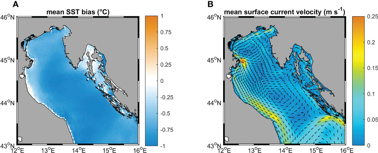
Figure 3 (A) mean SST bias; (B) surface circulation patterns, color map indicates the current speed, vectors (subsampled every 3 cell grids and normalized on the current speed) indicate the current directions.
The vertical structure of the water column reproduces the space-averaged temperature and salinity seasonal profiles presented by Artegiani et al. (1997a), and the surface circulation pattern (Figure 3B) captures, at least qualitatively, the main features of the gyre system characterizing the basin-scale circulation in the area (Artegiani et al., 1997b).
Light at the sea bottom was retrieved from Bio-Oracle (Tyberghein et al., 2012; Assis et al., 2018). Phosphate and nitrate concentrations were extracted from the Copernicus Marine Service (hereafter CMEMS). For the first step of the modelling phase (HIS) data from ROMS and CMEMS were sampled and averaged for the period between 1999 and 2018, whereas data extracted from Bio-Oracle were averaged from 2000 to 2014. The SCE simulation was driven by projected data of temperature, salinity, and current velocity fields at the sea bottom from ROMS model in the period between 2070 - 2099. For Random Forest and MaxEnt applications, all the variables were sampled on the same grid with 0.02° resolution, bracketing a geographical domain between 44.8-46 latitude and 23-14 longitude and projection (WGS84), interpolated when necessary using the “nearest neighbor” method. The patterns of the six environmental variables used in the study, with variations of temperature, salinity, and velocity in climate change scenarios, are reported in Figure 4.
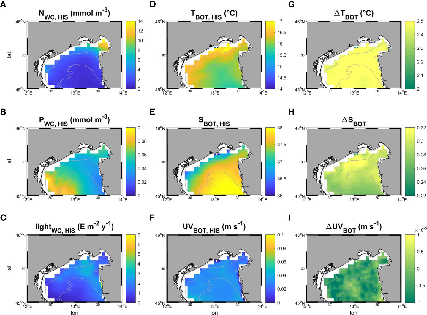
Figure 4 Patterns of the six environmental variables employed in this study. (A–F) show respectively the time averaged patterns of nitrate and phosphate concentration along the water column, and light, temperature, salinity and velocity at the sea bottom in the historical period (1999-2018). (G–I) map the difference (Δ) in bottom temperature, salinity and current velocity speed between future (under a severe climate change scenario RCP 8.5, 2070-2099 – SCE) and historical conditions (HIS).
2.4 Habitat Suitability Models set up and evaluation
Random Forest is an extension of single Classification Trees, in which multiple decision trees are built with random subsets of the data. This model can be employed for both classification and regression tasks (Vincenzi et al., 2011). Both modes were applied in this study, respectively for the identification of the unclassified habitats and for the computation of the suitability of each habitat, both in historical and climate change conditions. MaxEnt aims at assessing the suitability of a given habitat by pursuing a maximum entropy configuration (that is, closest to uniform) compatible with the available information (Freeman et al., 2013). Both models were populated with presence-only data of habitat-categorized coralligenous outcrops, using the six continuous environmental variables as predictors.
Before performing any suitability analyses, a tuning of hyperparameters in Random Forest (top parameters controlling the learning process and involved in understanding which parameters can correctly map the features) and parameters in MaxEnt (internal to the model and estimated by the training process, that explicates the system variability) is strongly suggested to define the optimal model architecture. In this study, the default set up of Random Forest implemented in R appeared adequate, while for MaxEnt a specific investigation was conducted with the ENMeval R package (version 0.3.1, Muscarella et al., 2014) determining the best options balancing goodness-of-fit and model complexity.
In both models, the suitability analyses were carried out using training and testing datasets including respectively 70% and 30% of the whole occurrence data. The training set enabled the model to learn the relations between the environmental variables and occurrences, while the testing set was used to evaluate the model performance. The goodness-of-fit and performance were quantified by using the “Area Under the Curve” (hereafter AUC) and “True Skill Statistic” (hereafter TSS), two metrics that proved to be particularly indicated for Random Forest regression and MaxEnt applications (Shabani et al., 2018; Acharya et al., 2019; Rew et al., 2020). The AUC, related to the probability that a randomly chosen occurrence site ranks more suitable than a randomly chosen absence site (Elith et al., 2006), ranges between 0 and 1, where 1 means perfect matching, 0.5 represents matching not better than random, and 0 corresponds to completely wrong predictions. TSS considers omission and commission errors (related to false negatives and false positives respectively) and is not affected by the size of the validation set. It ranges between -1 and +1, where +1 indicates a perfect agreement and values of 0 or less indicate performance no better than random (Allouche et al., 2006).
The relative contribution to the model predictions from each variable is quantified in Random Forest as the Mean Decrease Accuracy (hereafter %IncMSE), and in MaxEnt as the Permutation Importance. In both cases, higher values correspond to the higher importance of the variable.
In MaxEnt the Jackknife analysis also allows the quantification of the individual effect of each variable by systematically excluding it from the dataset (Elith et al., 2011). The use of this function helped to identify also the variables that mainly affect the model fit.
For both models, the suitability is expressed as a probability ranging from 0 (worst suitability for the habitat) to 1 (best suitability for the habitat).
2.5 Habitat area calculation, distribution, and shift
The raster files produced by each model were used to estimate the suitability in the historical period and under climate change RCP 8.5 scenario. The calculation of the surface of each range of suitability was conducted by implementing basic functions in R. Furthermore, the SCE suitability values were extrapolated, for each occurrence point, to hypothesize which habitat could be the most likely to be found according to the predicted changes in environmental variables.
The model outputs, provided as ASCII raster files, were post-processed using Matlab (version MatlabR2018a) to identify spatial patterns of change in habitat suitability, shifts in dominant habitat, and to produce maps for a visual representation of the results throughout the study area.
2.6 Sensitivity analysis
In order to explore how the uncertainty on the evolution of the environmental variables can affect the results of the present work, a sensitivity analysis was performed by running a set of additional HSM simulations in the future scenario, in which the projected values of each environmental variable were singularly increased and decreased by an estimate of the related uncertainty. The amount of this perturbation was defined based on existing large-scale modelling projections or, if unavailable, from information on basin-scale variability in present conditions (Bonaldo et al., 2014; Soto-Navarro et al., 2020; and Reale et al., 2022). For light radiation, in particular, the variation for the sensitivity analysis was chosen as the standard deviation of the present values restricted to a bathymetric range between -18 and -40m. A complete overview of the variations applied to each environmental factor is reported in Table 3. The overall sensitivity of the results was quantified in terms of consensus of the additional simulations with the SCE run. This was computed at each location as the fraction of sensitivity runs in which the projected evolution was consistent with the one computed in SCE. Larger values of consensus correspond to smaller sensitivity.
3 Results
3.1 Habitat classification
The classification of the reported occurrences into the three habitat assemblages results into two datasets differing from each other in only three occurrence points out of 85, reaching a 96% agreement rate. Figure 2 shows the distribution of the categorized record, while further details on the classification are provided in Supplementary Tables 1 and 2.
3.2 Models accuracy
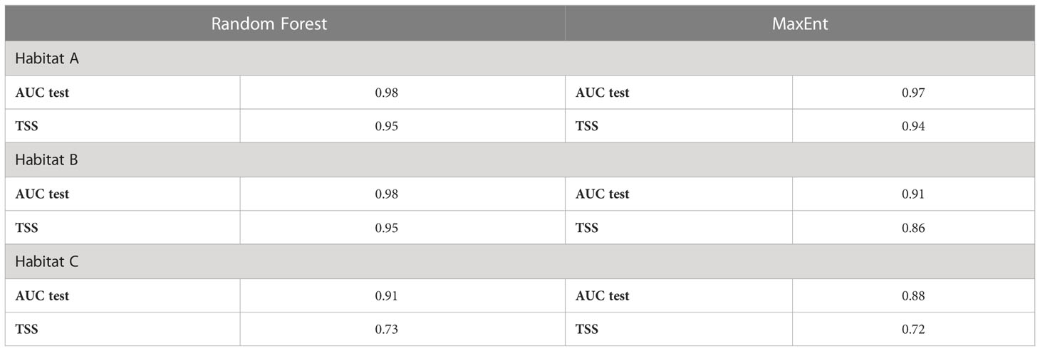
Both Random Forest and MaxEnt exhibit high AUC values (the lowest, 0.88, was calculated by MaxEnt for habitat C), meaning that the models have a high prediction accuracy (Table 4). Although Random Forest seems slightly better performing than MaxEnt according to this metric (Figure 5), the difference between models’ test AUC is very small (maximum 0.026 for habitat C). The models show high TSS values, indicating they were both reliable. Habitat A and B returned estimations of 0.95 for both in Random Forest and of 0.94 and 0.86 respectively in MaxEnt. Habitat C presents lower values with 0.73 and 0.72 in Random Forest and MaxEnt, respectively.
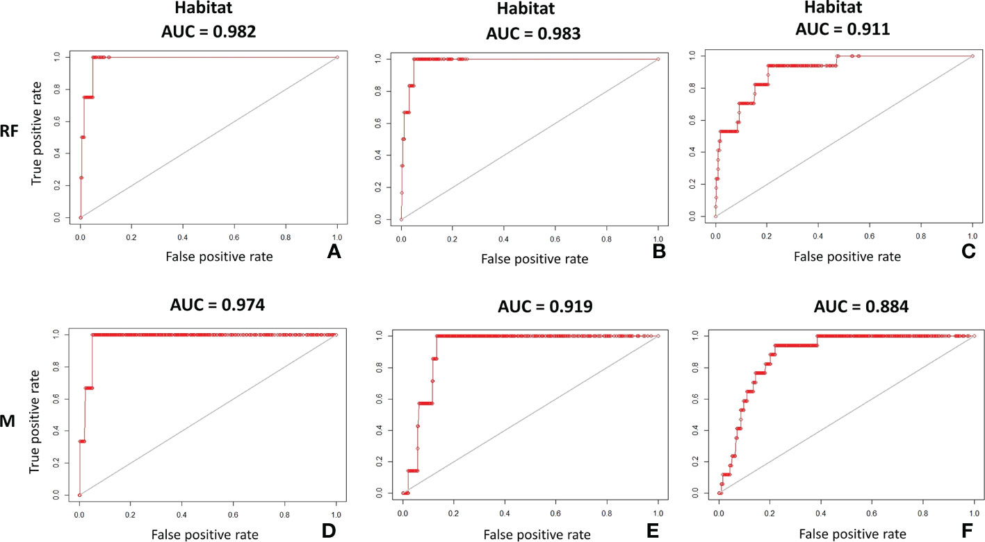
Figure 5 AUC plots on test dataset showing the accuracy of Random Forest (RF) and MaxEnt (M) in predicting the potential distribution of coralligenous: (A) Random Forest AUC on test dataset of habitat A; (B) Random Forest AUC on test dataset of habitat B; (C) Random Forest AUC on test dataset of habitat C; (D) MaxEnt AUC on test dataset of habitat A; (E) MaxEnt AUC on test dataset of habitat B; (F) MaxEnt AUC on test dataset of habitat C.
3.3 Variable importance and contribution
The analysis of the contribution of each environmental variable quantifies their role in controlling the habitat distribution. The evaluation of Random Forest features under the historical period highlights that for both habitats A and B the highest decrease in %IncMSE is observed when salinity is removed by the system (11.84% and 12.57%, respectively), followed by phosphate (4.24%) and nitrate (2.87%) for habitat A, and temperature and light (11.56% and 8.06%, respectively) for habitat B. Regarding habitat C, it appears that nitrate is the most influencing (19.94%) variable, followed by salinity (16.21%), and temperature (16.15%).
The MaxEnt analysis of contribution shows that the historical distribution of habitat A is largely dependent on temperature (99.3%). Habitat B is mainly influenced by temperature (47.1%) and phosphate (45.3%). In habitat C salinity is reported as the most contributing variable (71.3%), followed by nitrate (12.8%) and light (9.1%). A complete variable ranking and related figures are in Supplementary Tables 3–8, and Supplementary Figure 2.
The Jackknife analysis built-in in MaxEnt (Figure 6) shows that temperature in habitat A, when taken individually, is the most influencing the goodness-of-fit (referred to in the model as “gain”); once this variable is cut out, the gain decreases, suggesting that temperature was the main source of system’s variability. In habitat B, when considering each variable taken alone, light radiance appears as the one contributing the most, in turn, when individually removing each variable from the whole set, temperature emerges as the one mostly explaining the variability of the system. Salinity in habitat C is the most contributing variable when taken alone, but nitrate removal shows that this variable actually explains the variability of the system.
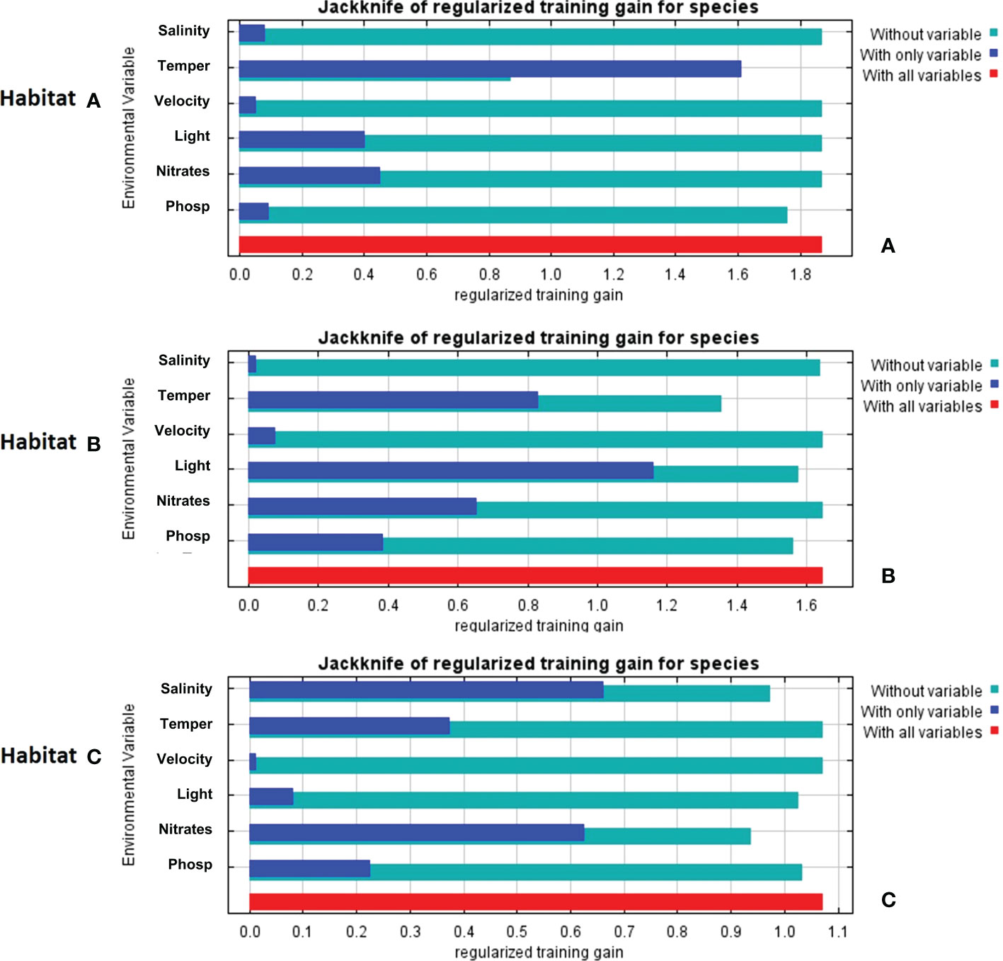
Figure 6 Jackknife analyses results derived from MaxEnt reporting the contribution and potential effects of variables on the model fit (referred in the system as “gain”): (A) Jackknife analysis of habitat A; (B) Jackknife analysis of habitat B; (C) Jackknife analysis of habitat C.
The response curves produced by MaxEnt reported for each habitat in Figures 7–9, represent the effect of each environmental variable on the model prediction. In habitat A, an increase in suitability is recorded as the light radiance increases and a similar trend is observed in habitat C where, however, the suitability curve reaches a maximum and decreases up to a plateau. Light in habitat B presents a bell-shaped curve meaning that an optimal range of suitability is present corresponding to a defined interval of values with zero suitability at the extremes of the distribution. Nitrate shows a similar trend to light, both in habitat A and B, whereas in habitat C high suitability values were reached at low concentrations. In both habitats A and B suitability is inversely related to phosphate concentration; in habitat C the highest suitability is obtained in correspondence to intermediate concentration values. Habitats A and B exhibit comparable trends also in response to salinity, both reporting a decrease from the optimal suitability (1.00) to 0.55 and 0.60 respectively as long as the variable increases. Habitat C reaches the highest suitability around 38 followed a sudden decrease for higher values. Increasing temperature in habitats A and B lead to an increase in their suitability, while in habitat C the highest value is reached at about 16.5°C, followed by a steep decrease. Finally, the increase in bottom current velocity in habitats A and B causes a constant decrease in suitability, whereas habitat C reaches the highest suitability at the midpoint of the current velocity curve.
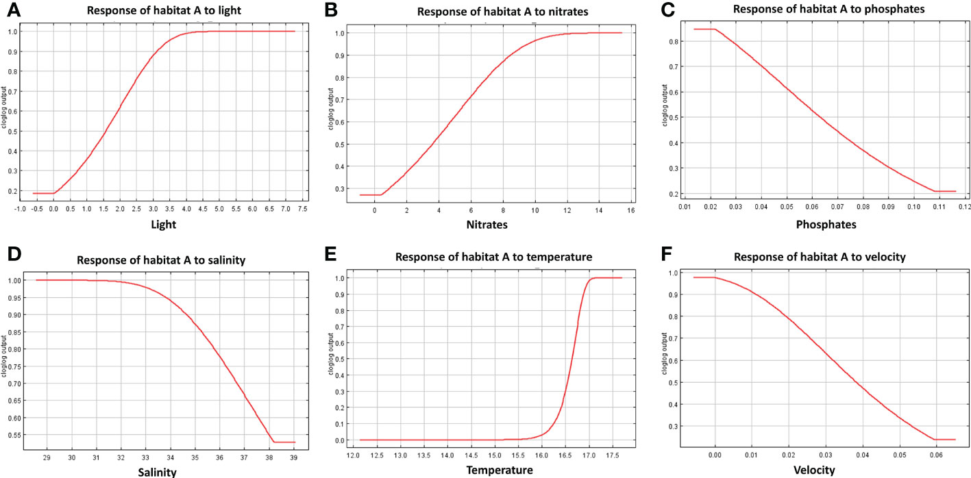
Figure 7 Response curves derived from MaxEnt reporting the relationship of predicted suitability of habitat A to environmental variables, with y-axis indicating the probability values and x-axis the concentration/intensity of the variables: (A) relationship between habitat A and light; (B) relationship between habitat A and nitrate concentration; (C) relationship between habitat A and phosphate; (D) relationship between habitat A and salinity; (E) relationship between habitat A and temperature; (F) relationship between habitat A and velocity.
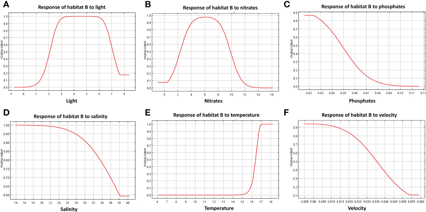
Figure 8 Response curves derived from MaxEnt reporting the relationship of predicted suitability of habitat B to environmental variables, with y-axis indicating the probability values and x-axis the concentration/intensity of the variables: (A) relationship between habitat B and light; (B) relationship between habitat B and nitrate concentration; (C) relationship between habitat B and phosphate; (D) relationship between habitat B and salinity; (E) relationship between habitat B and temperature; (F) relationship between habitat B and velocity.
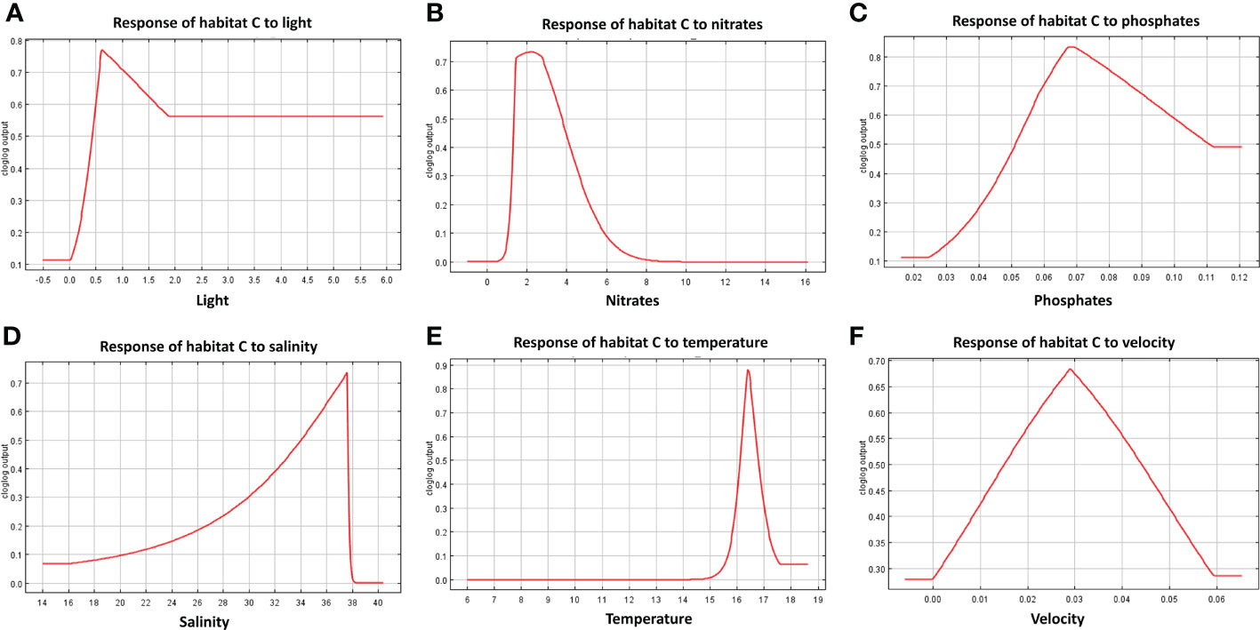
Figure 9 Response curves derived from MaxEnt reporting the relationship of predicted suitability of habitat C to environmental variables, with y-axis indicating the probability values and x-axis the concentration/intensity of the variables: (A) relationship between habitat C and light; (B) relationship between habitat C and nitrate concentration; (C) relationship between habitat C and phosphate; (D) relationship between habitat C and salinity; (E) relationship between habitat C and temperature; (F) relationship between habitat C and current velocity.
3.4 Coralligenous suitability mapping
Figures 10, 11 show the maps of historical suitabilities and the future variations computed respectively by Random Forest and MaxEnt for all habitat assemblages. In the historical run, Random Forest predicts patchy high suitability areas close to the occurrence point for all the three coralligenous habitat types, whereas MaxEnt predicts a wider suitable areas and smoother suitability patterns.
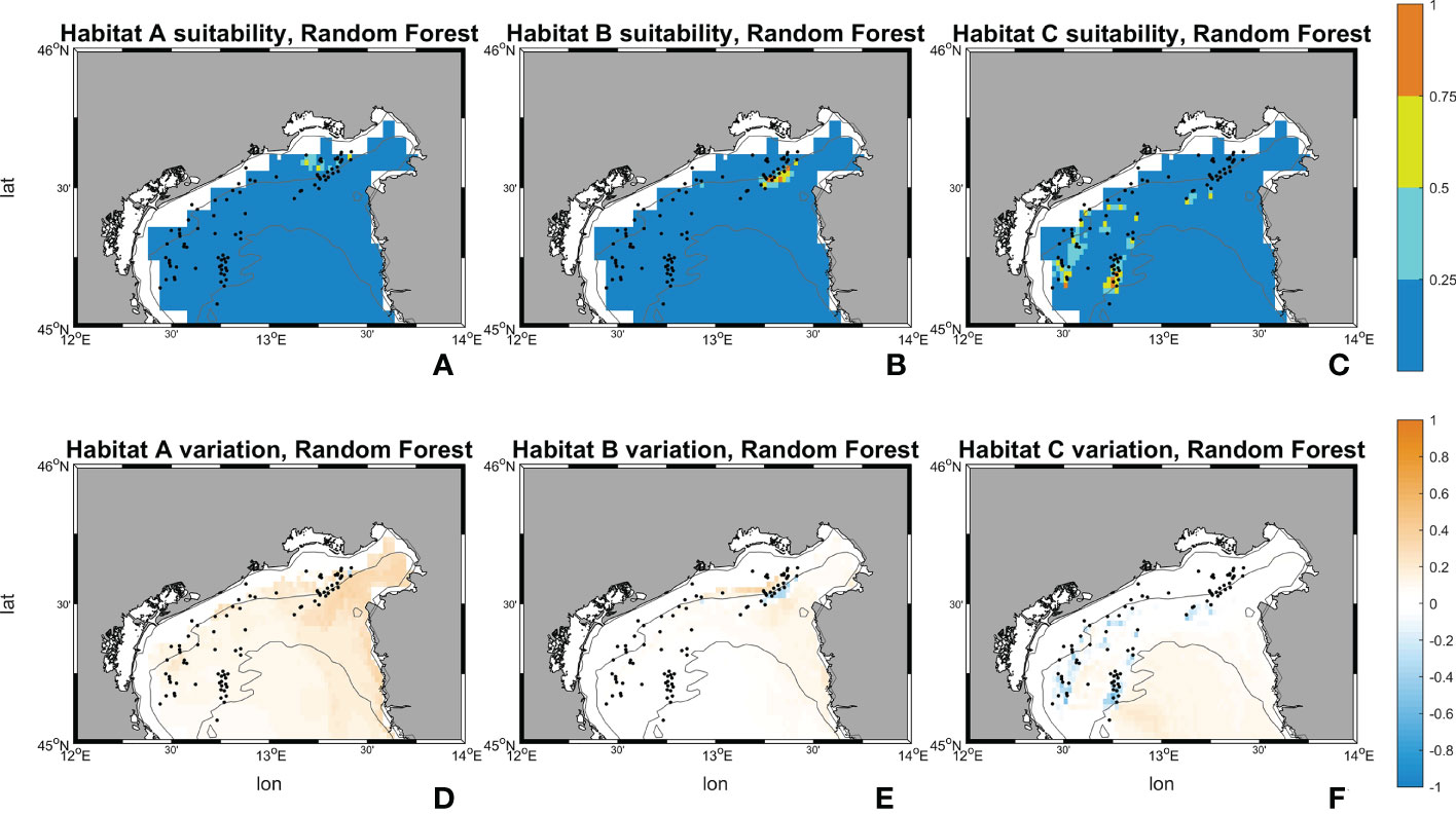
Figure 10 Suitability maps (horizontal resolution 0.02°) from Random Forest. Maps (A–C) represents Random Forest suitability for habitat A, B and C during the historical period (1999-2018). Maps (D–F) represents Random Forest future changes according to climate change RCP 8.5 scenario. First line scale legend: 0-0.25 = Low suitability; 0.25-0.5 = Moderate suitability; 0.5-0.75 = High suitability; 0.75-1 = Very high suitability (Thuiller and Münkemüller, 2010; Mousazade et al., 2019). Second line scale legend: -1 = prediction of a suitability decrement in comparison to historical period; 0 = no changes predicted; +1 = prediction of a suitability increment in comparison to historical period.
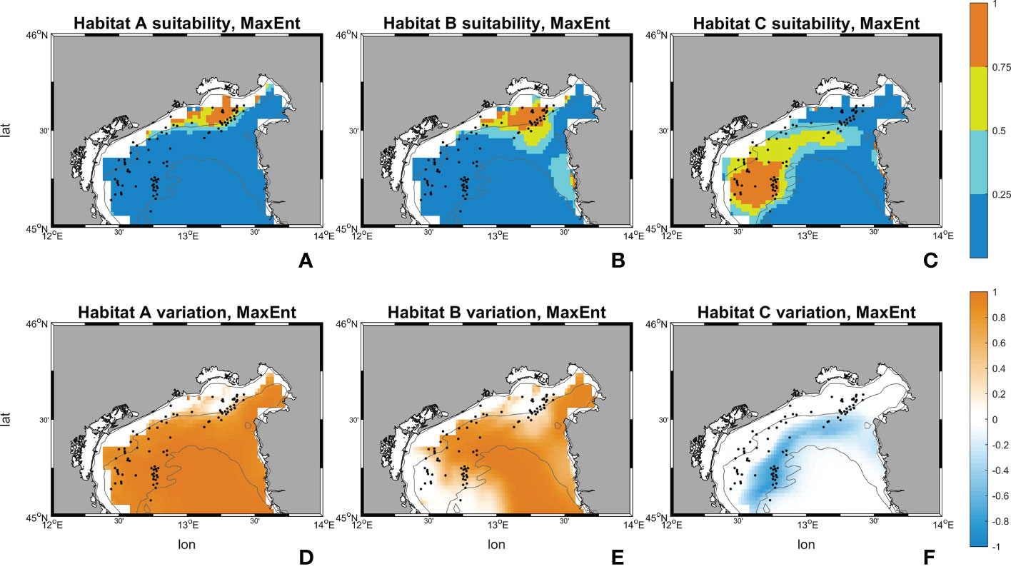
Figure 11 Suitability maps (horizontal resolution 0.02°) from MaxEnt. Maps (A–C) represents MaxEnt suitability for habitat A, B and C during the historical period (1999-2018). Maps (D–F) represents MaxEnt future changes according to climate change RCP 8.5 scenario. First line scale legend: 0-0.25 = Low suitability; 0.25-0.5 = Moderate suitability; 0.5-0.75 = High suitability; 0.75-1 = Very high suitability (Thuiller and Münkemüller, 2010; Mousazade et al., 2019). Second line scale legend: -1 = prediction of a suitability decrement in comparison to historical period; 0 = no changes predicted; +1 = prediction of a suitability increment in comparison to historical period.
Random Forest for habitat A in SCE predicts an increase in the probability of having ideal conditions in the whole area of interest, in particular towards the Gulf of Trieste, the Slovenian and Croatian coasts. Variations between the historical and SCE are considered here as changes in total area of each habitat. Areas with “low” (equal to suitability values comprehended between 0 and 0.25) and “high” (0.50 – 0.75) ranges experience an overall decrease of -801 km2 (-10.46%) and -3 km2 (-33.32%), whereas a very marked increase for the “moderate” (0.25 - 0.50) interval is reported with +805 km2 (+2121.41%). An increment in the suitability is shown also for habitat B. Random Forest reports an increase in the “moderate” interval with +117 km2 (equal to +339.92%) whereas the “low” surface decreases by -79 km2 (-1.04%) and “high” and “very high” (0.75 – 1.00) disappear in SCE. Lastly, in habitat C an overall decrease in suitability is observed in the SCE. Random Forest shows a decrease in the areas close to the occurrences and predicts a slight increase offshore. The variations between historical and SCE return an increment of +208 km2 (+2.80%) in the “low” range, but an important decrease is reported for the “moderate” range with -114 km2 (-65.99%), and the other two intervals set to zero.
Results from MaxEnt for habitat A exhibits a decrement in “low”, “moderate” and “high” percentage by -7069 km2 (99.56%), -228 km2 (-100%), and -99 km2 (-61.29%) respectively, whereas the “very high” increases by +7396 km2 (+3348.69%). Habitat B has an increment in “high” and “very high” ranges with +130 km2 and +4868 km2 (+43.47% and +1740.95%) respectively. “low” and “moderate” decrease by -4835 km2 and -164 km2 (-73.90% and -27.89%). Then, for habitat C MaxEnt returns a reversed pattern: only the lowest range reports an increase with +1213 km2 (+22.12%), the others decreased by -395 km2, -363 km2, and -454 km2 (-48.31%, -46.02%, -73.60%).
3.5 Habitat distribution and habitat shift
The comparison of the suitability values allows to identify the dominant (that is, the most suitable) habitat at each location, the habitat shift in future conditions, as well as the areas in which a minimum suitability threshold (in this case 0.5) is achieved (Figure 12).
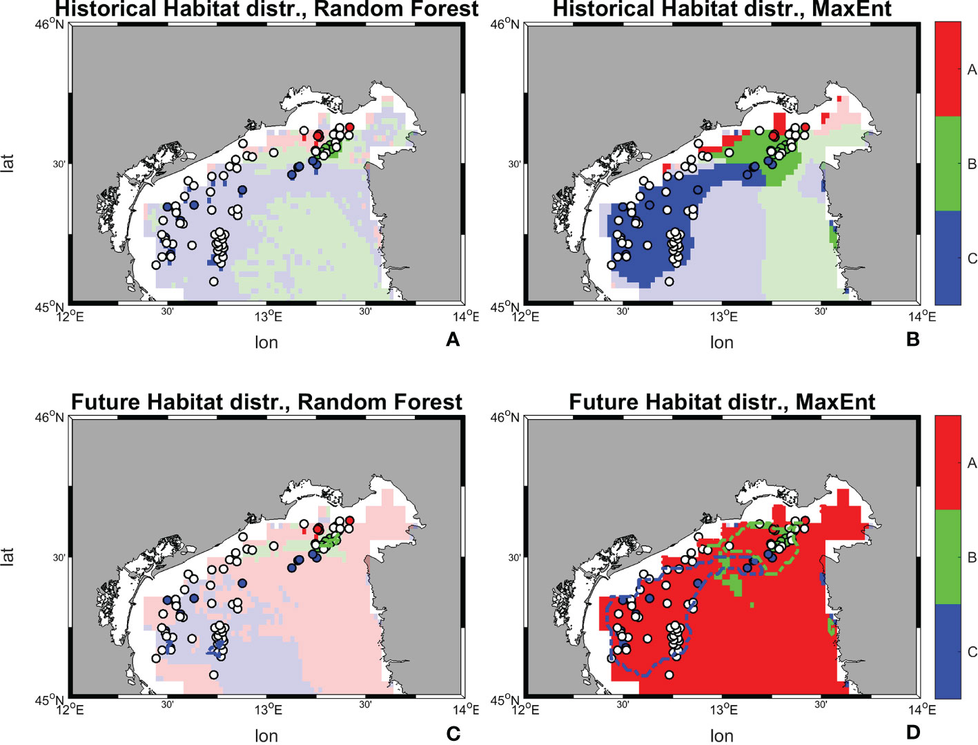
Figure 12 Historical and future distribution of dominant habitats (maximum suitability) according to Random Forest and MaxEnt models. (A) Historical distribution of habitats predicted by Random Forest; (B) Historical distribution of habitats predicted by MaxEnt; (C) Future distribution of habitats predicted by Random Forest; (D) Future distribution of habitats predicted by MaxEnt. Shaded colors indicate suitability values below a threshold of 0.5, therefore belonging to low-medium ranges, while marked ones stood for values above 0.5 and belonging to high range.
The results from Random Forest returns suitability below 0.5 on the whole study area for all three habitats. Although with relatively low suitability values, in the historical period habitat C seems to dominate over a larger area, followed by B and A. The result reverses in SCE, with habitat A occupying a wider suitability surface, followed by C, and B. This change in dominant habitat patterns is associated with 14 occurrence points possibly shifting from habitat C to A, 3 from B to A, and 1 from A to B. MaxEnt maps returns suitability both below and above the 0.5 threshold in the historical period, with higher values near the coastal zone. The habitat that coveres most of the area is habitat C, followed by B and A. Once again, the picture changes in SCE, with a dominant presence of habitat A above the 0.5 threshold throughout the whole basin. In this perspective, MaxEnt predicts a potential shift of 50 occurrence points from C to A, 21 from B to A, and 4 from A to B.
3.6 Results from sensitivity analysis and consensus maps
The results of the sensitivity analysis are summarised in consensus maps showing, for every cell of the domain, the fraction of sensitivity runs in which the sign of the trend of the suitabilities (Figure 13) or the projected dominant habitats (Figure 14) confirm the results of the SCE run. Very high scores (yellow color) appear widespread for habitats A and B (Figures 13A, B, D, E) both in Random Forest and Maxent, suggesting a satisfactory robustness for these predictions throughout the whole domain. Some larger sensitivity is found for habitat C (Figures 13C, F), appearing in Random Forest as a patchy pattern of low-agreement regions, and, to a smaller extent, in MaxEnt as a slight decrease in consensus along the coast.
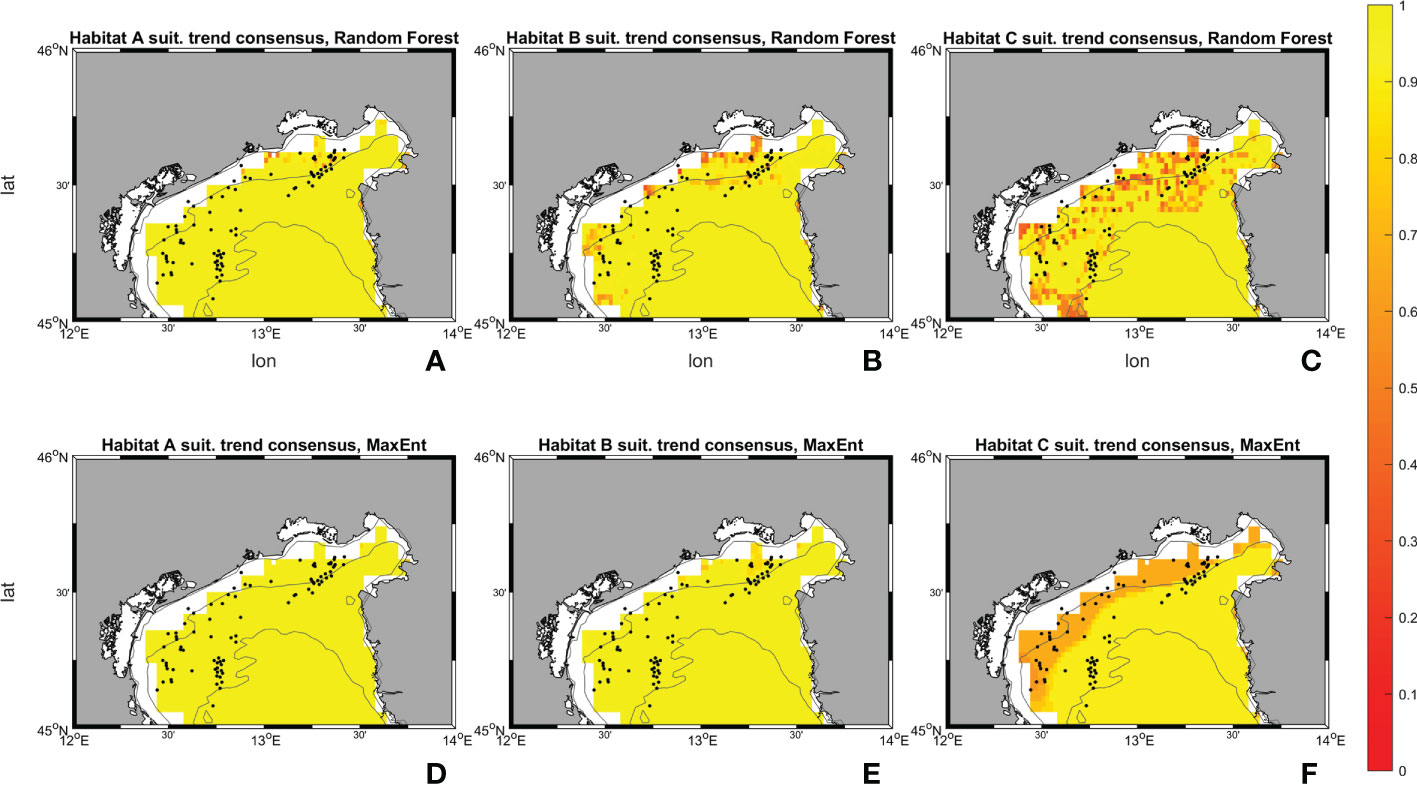
Figure 13 Consensus between trends sign in the sensitivity analysis and the SCE run for Random Forest (A–C) and for MaxEnt (D–F). For each simulation, agreement is assessed based only on the sign (either increasing or decreasing) of the trend. The scale ranges from 0 (worst agreement, no simulation in the sensitivity analysis in agreement with SCE) to 1 (perfect agreement, all simulations in agreement with SCE).
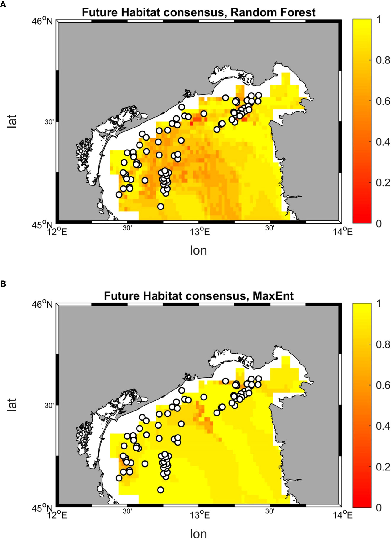
Figure 14 Consensus between projected habitat distribution in the sensitivity analysis and the SCE run for Random Forest (A) and MaxEnt (B).
The larger sensitivity of Random Forest in the calculation of the habitats suitabilites reflects on a smaller consensus in the prediction of the dominant habitat, whereas MaxEnt seems to confirm a larger robustness with respect to possible uncertainties in the environmental parameters (Figure 14).
4 Discussion
The identification of areas of priority for conservation and the successful management of Marine Protected Areas (hereafter MPAs), are severely hindered by a lack of data on the distribution of habitats identified as vulnerable and threatened by environmental and anthropogenic effects at different scales, as it is the case of the coralligenous (Teixidó et al., 2013; Marshall et al., 2014). MPAs are recognized as excellent tools to counteract some threats that affect marine ecosystems and decrease their vulnerability by enhancing their resilience (Vitelletti and Bonaldo, 2020). The prediction of the effects of climate change on environmental conditions and communities can feed the adoption of anticipatory approaches, thus fostering the effective management and protection of marine areas (Elliott et al., 2017). The application of HSMs can provide forecast on the effects of environmental processes and possible human actions on the marine environment, facilitating the identification of areas of priority for conservation, and supporting the definition and implementation of MPA management plans (Robinson et al., 2011).
4.1 Remarks on models performance
The accuracy metrics calculated for Random Forest and MaxEnt confirm in principle the good performance of both models in predicting the probability of coralligenous presence in the Northern Adriatic Sea (Acharya et al., 2019 and reference therein). Nonetheless, the appearing discrepancies in terms of present and future habitat distribution show that accuracy metrics per se are not always sufficient for drawing conclusions on the validity of the results. In fact, due to the complexity of the ecological processes and the unavoidable need for simplified conceptualizations (be them mechanistic or correlative), HSMs are intrinsically prone to different sources of error. Several studies have investigated the different relations between HSMs and input data characteristics concluding that models results and effectiveness vary according to the study system, data quality, and the scientific question addressed (Elith and Graham, 2008 and references therein). The implementation of at least two model techniques, with the comparison of their performances and the integration of the results, is typically adopted in HSM studies to better address the uncertainty related to the modelling approach.
The two models employed in this study predict higher habitats’ suitability in areas close to the available occurrences, albeit with different distributions. While MaxEnt reports larger surfaces suitable for coralligenous presence with a gradual decrease as moving away from the occurrences, Random Forest, at a finer scale observation, showed narrower suitability ranges. In future conditions, both models predict some changes in habitat suitability and dominance with more marked variations in MaxEnt than in Random Forest, although with overall comparable spatial patterns. However, it is clear that a net loss of suitable areas of some habitat types is envisaged by both models and some associated species are more vulnerable than others to climate change (Boys et al., 2021). The difference between MaxEnt and Random Forest results can be ascribed to various reasons, from the implementation of different approaches eliciting differences in behavior of species distribution outputs to the choice of environmental variables (Shabani et al, 2018 and reference therein). In particular, the patchy pattern in Random Forest is probably due to an overfitted model, where the effects of environmental conditions on the location of occurrences exert a greater influence on the closest surrounding area and consequently lead to the presence of high probabilities of suitability in the neightbouring cells. The configuration of a built-in option called “regularization parameter” in MaxEnt permits to prevent overfitting although with a less localized prediction (Phillips and Dudík, 2008 and reference therein). The absence of this option in Random Forest model can be the reason for the greater influence of the environmental variables on the records’ surrounding area and confirms the sensitivity of this model to spatial autocorrelation (Sinha et al., 2019). The size of the dataset might be another factor giving rise to different results between the models. Literature reports evidence of MaxEnt being capable of dealing with limited datasets (Kaky et al., 2020); whereas, Random Forest is more influenced by the quantity and spatial distribution of the available occurrences (Rahmati et al., 2016; Acharya et al., 2019), though possibly achieving satisfactory results also in the presence of a limited number of occurrence records (Mi et al., 2017 and reference therein). Even though the model skills of the two approachs are comparable, the tendency to overfitting in Random Forest, combined with its overall higher sensitivity to uncertainties in the input data, suggests that present and projected basin-scale patterns produced by this model should be treated with higher cautiousness.
4.2 Habitat shifts and ecological implications
The differentiation into the three habitat types and the application of HSMs allows to predict how each of them will be influenced by future climate changes.
Among the considered environmental variables temperature, salinity and nitrate are the strongest drivers for the distribution of the three habitats types. These variables are largely influenced by atmospheric factors as well as by the terrestrial dynamics of the North Adriatic Sea that is subject to important river inputs (Degobbis et al., 2000). Alterations in environmental variables due to climate change have already been explored and have proved to be relevant in this sub-basin being able to change the characteristics and quality of the water body (Rizzi et al., 2016). However, a certain degree of correlation among variables, particularly in coastal environments dominated by cross-shore gradients, may have some spurious impacts on the results (Burbach, 2011) also considering that the distribution of habitats is influenced by overlapping and integrating factors. For this reason, during the setting up phase of any model, it is recommended to settle the correct resolution and spatial scale to capture the entire available environmental variability.
The results obtained in this study predict the shift from habitats B and C to habitat A, suggesting a more suitable growth conditions for habitat A species assemblages in the future. Opportunistic organisms (e.g. turf-forming macroalgae, encrusting Porifera, and bioeroders) dominate habitat A and are known to tolerate what is generally considered stressful environmental conditions, such as high temperature and organic loads (Piazzi et al., 2012; Falace et al., 2015). Indeed, the suitability distribution of this habitat was positively correlated with high nitrate concentrations and temperature, while a negative influence resulted from high salinity and phosphate levels. These results are in line with previous modeling findings (Falace et al., 2015). Habitat B is considered a transitional habitat, being composed of species characterizing habitat A together with massive Porifera, erect tunicate, and non-calcareous encrusting algae. Similarly to A, habitat B distribution appears influenced by temperature and salinity showing respectively positive and negative relationships. Both the increments of phosphate and nitrate concentrations have a negative influence on the potential presence of habitat B. These results are realistic considering the negative impact that high loads of nutrients and suspended sediment (which are highly correlated with dissolved nutrients) have on erect and filter-feeders organisms, by hindering their breathing and feeding habit (Lemly, 1982; Gibson et al., 2006 and reference therein). Finally, habitat C, distributed farther from the coast as compared to the other two, is characterized by the presence of calcareous algae and the tunicate Polycitor adriaticus, a species observed mainly in undisturbed environments and vulnerable to stressful conditions (Falace et al., 2015). Indeed, this habitat presents higher suitability in the Northern-Western Adriatic at low-medium concentrations of nutrients and medium-low temperatures (around 16.5°C). Light at the sea bottom (influenced by water turbidity) slightly influences the distribution of the different habitats, especially B and C. This result finds consistency in previous studies identifying light radiation as a factor that influences the distribution of mesophotic communities (Rossi et al., 2017; Coppari et al., 2020; Castellan et al., 2022), as the northern Adriatic rocky outcrops are defined (Fava et al., 2016; Ingrosso et al., 2018).
Under the climate change scenario, an average temperature increase of 2.48°C in the sub-basin is predicted. The changes in this environmental variable result in a sharp decline (Random Forest) or disappearance (MaxEnt) of habitat C (and partly of habitat B), which could be replaced by habitat A. The resulting pattern is opposite to what is depicted in the historical period. Since habitat A is dominated by opportunistic macroalgae, it is not surprising that it can benefit from sea warming thus expanding its area at the expense of more temperature-vulnerable habitat-forming species, such as massive Porifera and erect tunicates (Ji et al., 2016; Ober, 2016). Extreme warming events caused by climate change have been observed to have major impacts on Mediterranean coralligenous assemblages, inducing the loss of engineering species characterized by key functional traits, which have a role in driving the biogeochemical cycles and the trophic chain that support biodiversity (Gómez-Gras et al., 2021).
It is interesting to know that contrasting observations have been reported about the effects of seawater warming on crustose coralline algae (associated with habitat C) (Cornwall et al., 2019). Unfortunately, in this study, it was not possible to discriminate the rocky outcrops based on their coralline algae species composition (mainly Lithophyllum stictaeforme, Lithothamnion minervae, and Peyssonnelia polymorpha according to Ponti et al., 2011).
An intensification of studies coupling long-term monitoring of coralligenous communities with habitat suitability and climate model predictions would be strongly beneficial in filling the present scarcity of an evidence-based insight in the effects of warming on these species (see, for example, Rodríguez-Prieto, 2016), Furthermore, in combination with warming, cumulative negative effects are expected on coralligenous. Indeed fast-growing turfs and invasive algae can overgrow on crustose coralline algae and trap and accumulate sediment preventing the recovery of filter feeders, leading then to the declining of these species due to high sedimentation rate (Filbee-Dexter et al., 2016 and references therein).
The projected scenario depicts a severe simplification in coralligenous habitat and a general loss of assemblages over the entire study area. Worth noting, the apparent underestimate of the SST increase rate in the ocean model simulation could imply, under the assumption that in shallow waters this reflects to some extent the behavior of the whole water column, that our projections underestimate the intensity of the climate change signal. As a result, the conditions discussed here for the end of this century could take place significantly sooner than depicted in this study. How climate change will alter the physical and chemical properties of the North Adriatic sub-basin and sedimentation loads is still unclear, even though changes in riverine inputs and runoff are expected, due to altered precipitations and snow-ice melting, together with increased frequency of storm surges (Castellan et al., 2022). The combined effect of all these events is uncertain, but surely it will alter the water quality and turbidity of the basin, with consequences on the species influenced by light radiation (Rizzi et al., 2016; Castellan et al., 2022), as those associated to habitat B and C. Nonetheless, the sensitivity analysis shows that the overall picture emerging from the present work can be confirmed even when accounting for the uncertainty affecting the values of the environmental parameters.
The biodiversity loss expected for the Northern Adriatic Sea in climate change conditions will likely lead to the loss of key ecological processes with important consequences on the entire food web and ecosystem functioning.
5 Conclusions
The use of HSMs is achieving a major role in estimating potential habitat distributions and informing conservation strategies. As such, these modeling tools can support environmental surveys planning and management decisions and can suggest more suitable locations where conservation efforts should be focused. At present the available knowledge on HSM applications provides no striking evidence of one approach clearly outperforming the others for any application: for this reason, it is generally a good strategy to apply different approaches and critically evaluate the reliability of their results.
With reference to the present application, the following conclusions can be drawn:
● both Random Forest and MaxEnt achieved satisfactory accuracy metrics for the analysis of coralligenous habitats in the Northern Adriatic Sea. Nonetheless, some tendency to overfitting reported in the former, together with its higher sensitivity to uncertain input data, suggest some cautionsness in the interpretation of its results, particularly for spatial patterns far of the occurrence locations;
● the application of these HSMs showed that widespread modifications in coralligenous habitat distributions should be expected in a severe climate change condition (RCP 8.5). Tolerant and opportunistic species are expected to expand their distribution in the Northern Adriatic Sea, while calcareous species and organisms more vulnerable to environmental alterations might undergo a decrease in their suitable habitat;
● the projected shift in habitat distribution will result in a a potential net loss of biodiversity in the sub-basin;
● in this perspective, the use of HSMs can facilitate the identification of protection priorities for endangered areas. To this aim, the intensification of survey activities and the definition of long-term monitoring plans would provide valuable data for the model applications, collecting at the same time information on the evolution of marine habitats and on the results of management and protection actions put in place in these systems.
Data availability statement
Publicly available datasets were analyzed in this study. This data can be found here: Environmental data: - CMEMS data: Teruzzi, A., Di Biagio, V., Feudale, L., Bolzon, G., Lazzari, P., Salon, S., et al. (2021). Mediterranean Sea Biogeochemical reanalysis (CMEMS MED-biogeochemistry, MedBFM3 system) (Version 1) set. Copernicus Monit. Environ. Mar. Service (CMEMS). doi: 10.25423/CMCC/MEDSEA_MULTIYEAR_BGC_006_008_MEDBFM3 available at https://resources.marine.copernicus.eu/product-detail/MEDSEA_MULTIYEAR_BGC_006_008/INFORMATION - Bio-Oracle data: Tyberghein, L., Verbruggen, H., Pauly, K., Troupin, C., Mineur, F. and De Clerck, O. (2012), Bio-ORACLE: a global environmental dataset for marine species distribution modelling. Global Ecology and Biogeography, 21: 272-281. https://doi.org/10.1111/j.1466-8238.2011.00656.x; Assis, J, Tyberghein, L, Bosch, S, Verbruggen, H, Serrão, EA, De Clerck, O. Bio-ORACLE v2.0: Extending marine data layers for bioclimatic modelling. Global Ecol Biogeogr. 2018; 27: 277– 284. https://doi.org/10.1111/geb.12693 - Occurrences data: Ponti, M., Colosio, F., Tumedei, M., and Abbiati, M. (2005). “Popolamenti Epibentonici Delle Tegnùe Chioggia”, in Atti Del 1° Convegno Subacquea & Ambiente: Le Tegnùe Di Chioggia, 17-18 Settembre 2005, 33–41; Martin, C.S., Giannoulaki, M., De Leo, F., Scardi, M., Salomidi, M., Knittweis, L., Pace, M.L., Garofalo, G., Gristina, M., Ballesteros, E., Bavestrello, G., Belluscio, A., Cebrian, E., Gerakaris, V., Pergent, G., Pergent-Martini, C., Schembri, P. J., Terribile, K., Rizzo, L., Ben Souissi, J., Bonacorsi, M., Guarnieri, G., Krzelj, M., Macic, V., Punzo, E., Valavanis V., and Fraschetti, S. (2014). Coralligenous and maerl habitats: predictive modelling to identify their spatial distributions across the Mediterranean Sea. Science, Engineering and Humanities and Social Sciences references, 4, 5073. doi: 10.1038/srep05073; Falace, A., Kaleb, S., Curiel, D., Miotti, C., Galli, G., Querin, S., Ballesteros, E., Solidoro, C., and Bandelj, V. (2015). Calcareous bio-concretions in the Northern Adriatic Sea: Habitat types, environmental factors that influence Habitat distributions, and predictive modeling. PLoS ONE, 10(11), 1–21. doi: 10.1371/journal.pone.0140931.
Author contributions
The authors confirm their contribution to the paper as follows: MV and DB conceived the study. MV, EM, LB, and DB collected and analyzed the data. MV, DB, AR, and LS performed the modeling with the support of EM and BL. MV, DB, EM, AR, LS, and LB interpreted the results and contributed to the original draft and the editing. All authors contributed to the article and approved the submitted version.
Funding
This work was partially supported by the Interreg project AdriaClim (Climate change information, monitoring and management tools for adaptation strategies in Adriatic coastal areas; project ID 10252001) funded by the European Union under the V-A Interreg Italy-Croatia CBC programme.
Acknowledgments
Authors are grateful to S. Pepi for his invaluable help in the statistical analysis.
Conflict of interest
The authors declare that the research was conducted in the absence of any commercial or financial relationships that could be construed as a potential conflict of interest.
Publisher’s note
All claims expressed in this article are solely those of the authors and do not necessarily represent those of their affiliated organizations, or those of the publisher, the editors and the reviewers. Any product that may be evaluated in this article, or claim that may be made by its manufacturer, is not guaranteed or endorsed by the publisher.
Supplementary material
The Supplementary Material for this article can be found online at: https://www.frontiersin.org/articles/10.3389/fmars.2023.1050293/full#supplementary-material
References
Acharya B. K., Chen W., Ruan Z., Pant G. P., Yang Y., Shah L. P., et al. (2019). Mapping environmental suitability of scrub typhus in Nepal using MaxEnt and random forest models. Int. J. Environ. Res. Public Health 16 (23), 4845. doi: 10.3390/IJERPH16234845
Allouche O., Tsoar A., Kadmon R. (2006). Assessing the accuracy of species distribution models: prevalence, kappa and the true skill statistic (TSS). J. Appl. Ecol. 43 (6), 1223–1232. doi: 10.1111/J.1365-2664.2006.01214.X
Artegiani A., Bregant D., Paschini E., Pinardi N., Raicich F., Russo A. (1997a). The Adriatic Sea general circulation. part I: Air–Sea interactions and water mass structure. J. Phys. Oceanogr. 27, 1492–1514. doi: 10.1175/1520-0485(1997)027<1492:TASGCP>2.0.CO;2
Artegiani A., Bregant D., Paschini E., Pinardi N., Raicich F., Russo A. (1997b). The Adriatic Sea general circulation. part II: Baroclinic circulation structure. J. Phys. Oceanogr. 27, 1515–1532. doi: 10.1175/1520-0485(1997)027<1515:TASGCP>2.0.CO;2
Assis J., Tyberghein L., Bosch S., Verbruggen H., Serrão E. A., De Clerck O. (2018). Bio-ORACLE v2.0: Extending marine data layers for bioclimatic modelling. Global Ecol. Biogeogr. 27, 277–284. doi: 10.1111/geb.12693
Barbier E. B. (2017). Marine ecosystem services. Curr. Biol. 27 (11), R507–R510. doi: 10.1016/j.cub.2017.03.020
Bates A. E., McKelvie C. M., Sorte C. J., Morley S. A., Jones N. A., Mondon J. A., et al. (2013). Geographical range, heat tolerance and invasion success in aquatic species. Proc. R. Soc. B: Biol. Sci. 280 (1772), 20131958. doi: 10.1098/rspb.2013.1958
Behrenfeld M. J., O’Malley R. T., Siegel D. A., McClain C. R., Sarmiento J. L., Feldman G. C., et al. (2006). Climate-driven trends in contemporary ocean productivity. Nature 444, 752–755. doi: 10.1038/NATURE05317
Bonaldo D., Benetazzo A., Bergamasco A., Falcieri F. M., Carniel S., Aurighi M., et al. (2014). Sediment transport modifications induced by submerged artificial reef systems: A case study for the gulf of Venice. Oceanological Hydrobiological Stud. 43 (1), 7–20. doi: 10.2478/s13545-014-0112-4
Boys W. A., Siepielski A. M., Smith B. D., Patten M. A., Bried J. T. (2021). Predicting the distributions of regional endemic dragonflies using a combined model approach. Insect Conserv. Diversity. 14 (1), 52–66. doi: 10.1111/ICAD.12444
Burbach T. (2011). The influence of environmental variables on predicting rare-plant habitat in the nez perce national forest. Master's thesis, University of Montana.
Cahill A. E., Aiello-Lammens M. E., Fisher-Reid M. C., Hua X., Karanewsky C. J., Ryu H. Y., et al. (2012). How does climate change cause extinction? Procedings R. Soc. B: Biol. Sci. 280 (1750).
Cañadas A., Sagarminaga R., Stephanis R. D., Urquiola E., Hammond P. S. (2005). Habitat preference modelling as a conservation tool: proposals for marine protected areas for cetaceans in southern Spanish waters. Aquat. Conserv. Mar. Freshw. Ecosyst. 15, 495–521. doi: 10.1002/aqc.689
Casellato S., Masiero L., Sichirollo E., Soresi S. (2007). Hidden secrets of the northern Adriatic: “Tegnúe”, peculiar reefs. Cent. Eur. J. Biol. 2, 122–136. doi: 10.2478/s11535-007-0004-3
Casellato S., Stefanon A. (2008). Coralligenous habitat in the northern Adriatic Sea: An overview. Mar. Ecol. 29 (3), 321–341. doi: 10.1111/j.1439-0485.2008.00236.x
Castellan G., Angeletti L., Montagna P., Taviani M. (2022). Drawing the borders of the mesophotic zone of the Mediterranean Sea using satellite data. Sci. Rep. 12 (1), 1–12. doi: 10.1038/s41598-022-09413-4
Cenci E., Mazzoldi C. (2006). Le tegnue di chioggia: Prima valutazione qualitative e quantitative della fauna ittica. Biol. Marina Mediterr. 13 (1), 840–843.
Cerrano C., Bavestrello G., Bianchi C. N., Calcinai B., Cattaneo-Vietti R., Morri C., et al. (2001). The role of sponge bioerosion in Mediterranean coralligenous accretion. In Mediterr. Ecosyst. (Milano) pp, 235–240).
Cheung W. W. L., Lam V. W. Y., Sarmiento J. L., Kearney K., Watson R., Pauly D. (2009). Projecting global marine biodiversity impacts under climate change scenarios. Fish Fisheries 10, 235–251. doi: 10.1111/j.1467-2979.2008.00315.x
Coll M., Piroddi C., Albouy C., Ben Rais Lasram F., Cheung W. W., Christensen V., et al. (2012). The Mediterranean Sea under siege: spatial overlap between marine biodiversity, cumulative threats and marine reserves. Global Ecol. Biogeogr. 21 (4), 465–480. doi: 10.1111/j.1466-8238.2011.00697.x
Compton T. J., Leathwick J. R., Inglis G. J. (2010). Thermogeography predicts the potential global range of the invasive European green crab (Carcinus maenas). Divers. Distrib. 16, 243–255. doi: 10.1111/j.1472-4642.2010.00644.x
Coppari M., Fumarola L., Bramanti L., Romans P., Pillot R., Bavestrello G., et al. (2020). Unveiling asexual reproductive traits in black corals: Polyp bail-out in antipathella subpinnata. Coral Reefs 39 (6), 1517–1523. doi: 10.1007/s00338-020-02018-1
Cornwall C. E., Diaz-Pulido G., Comeau S. (2019). Impacts of ocean warming on coralline algal calcification: Meta-analysis, knowledge gaps, and key recommendations for future research. Front. Mar. Sci. 6, 186. doi: 10.3389/fmars.2019.00186
Council Regulation (EC)(2006) Management measures for the sustainable exploitation of fishery resources in the Mediterranean Sea, amending regulation (EEC) no 2847/93 and repealing regulation (EC) no 1626/94, council regulation (EC) no 1967/2006 of 21 December. Available at: http://data.europa.eu/eli/reg/2006/1967/2019-08-14 (Accessed 10/01/2022).
Defforge C., Merlis T. (2017). Observed warming trend in sea surface temperature at tropical cyclone genesis. Geophys. Res. Lett. 44 (2), 1034–1040. doi: 10.1002/2016GL071045
de Francesco M. C., Chiuchiarelli I., Frate L., Carranza M. L., Pagliani T., Stanisci A. (2020). “Towards new marine-coastal natura 2000 sites in the central Adriatic Sea,” in Eighth international symposium “Monitoring of Mediterranean coastal areas. problems and measurement techniques. Eds. Bonara L., Carboni D., De Vincenzi M. Firenze University Press, 529–539.
Degobbis D., Precali R., Ivancic I., Smodlaka N., Fux D., Kveder S. (2000). Long-term changes in the northern Adriatic ecosystem related to anthropogenic eutrophication. Int. J. Environ. pollut. 13, 495–533. doi: 10.1504/IJEP.2000.002332
Degraer S., Verfaillie E., Willems W., Adriaens E., Vincx M., Van Lancker V. (2008). Habitat suitability modelling as a mapping tool for macrobenthic communities: an example from the Belgian part of the north Sea. Cont Shelf Res. 28, 369–379. doi: 10.1016/j.csr.2007.09.001
Deutsch C., Ferrel A., Seibel B., Pörtner H.-O., Huey R. B. (2015). Ecophysiology. Climate change tightens a metabolic constraint on marine habitats. Science 348 (6239), 1132–1135. doi: 10.1126/science.aaa1605
Doney S. C., Ruckelshaus M., Duffy E. J., Barry J. P., Chan F., English C. A., et al. (2012). Climate change impacts on marine ecosystems. Annu. Rev. Mar. Science. 4, 11–37. doi: 10.1146/annurev-marine-041911-111611
Elith J., Graham C. H. (2009). Do they? how do they? WHY do they differ? on finding reasons for differing performances of species distribution models. Ecography 32, 66–77. doi: 10.1111/j.1600-0587.2008.05505.x
Elith J., Graham C. H., Anderson R. P., Dudík M., Ferrier S., Guisan A., et al. (2006). Novel methods improve prediction of species’ distributions from occurrence data. Ecography 29, 129–151. doi: 10.1111/j.2006.0906-7590.04596.x
Elith J., Leathwick J. R. (2009). Species distribution models: Ecological explanation and prediction across space and time. Annu. Rev. Ecol. Evol. Syst. 40, 677–697. doi: 10.1146/annurev.ecolsys.110308.120159
Elith J., Phillips S. J., Hastie T., Dudík M., Chee Y. E., Yates C. J. (2011). A statistical explanation of MaxEnt for ecologists. Diversity Distributions 17 (1), 43–57. doi: 10.1111/j.1472-4642.2010.00725.x
Elliott M., Burdon D., Atkins J. P., Borja A., Cormier R., De Jonge V. N., et al. (2017). “And DPSIR begat DAPSI (W) r (M)!”-a unifying framework for marine environmental management. Mar. pollut. Bull. 118 (1-2), 27–40. doi: 10.1016/j.marpolbul.2017.03.049
European Commission (1992). Council directive 92/43/EEC of may 21 1992 on the conservation of natural habitats and of wild fauna and flora. Off. J. Eur. Communities 206, 22/07/1992, P. 0007–0050.
European Commission (2008). Directive 2008/56/EC of the European parliament of the council of 17 June 2008 establishing a framework for community action in the field of marine environmental policy (Marine strategy framework directive). Off. J. Eur. Union L164/19, 25/06/2008, P. 19–40.
Falace A., Kaleb S., Curiel D., Miotti C., Galli G., Querin S., et al. (2015). Calcareous bio-concretions in the northern Adriatic Sea: Habitat types, environmental factors that influence habitat distributions, and predictive modeling. PloS One 10 (11), 1–21. doi: 10.1371/journal.pone.0140931
Fava F., Ponti M., Abbiati M. (2016). Role of recruitment processes in structuring coralligenous benthic assemblages in the northern Adriatic continental shelf. PloS One 11 (10), e0163494. doi: 10.1371/journal.pone.0163494
Filbee-Dexter K., Feehan C. J., Scheibling R. E. (2016). Large-Scale degradation of a kelp ecosystem in an ocean warming hotspot. Mar. Ecol. Prog. Ser. 543, 141–152. doi: 10.3354/meps11554
Fraschetti S., Fabbrizzi E., Tamburello L., Uyarra M. C., Micheli F., Sala E., et al. (2022). An integrated assessment of the good environmental status of Mediterranean marine protected areas. J. Environ. Manage. 305, 114370. doi: 10.1016/j.jenvman.2021.114370
Freeman L. A., Kleypas J. A., Miller A. J. (2013). Coral reef habitat response to climate change scenarios. PloS One 8 (12), 1–14. doi: 10.1371/journal.pone.0082404
García Molinos J., Halpern B., Schoeman D., Brown C. J., Kiessling W., Moore P. J., et al. (2016). Climate velocity and the future global redistribution of marine biodiversity. Nat. Clim Change 6, 83–88. doi: 10.1038/nclimate2769
Garcia-Reyes M., Sydeman W., Schoeman D., Rykaczewski R., Black B., Smit A., et al. (2015). Under pressure: Climate change, upwelling, and eastern boundary upwelling ecosystems. Front. Mar. Sci. 2. doi: 10.3389/fmars.2015.00109
Giannoulaki M., Pyrounaki M. M., Bourdeix J. H., Ben Abdallah L., Bonanno A., Basilone G., et al. (2017). Habitat suitability modeling to identify the potential nursery grounds of the Atlantic mackerel and its relation to oceanographic conditions in the Mediterranean sea. Front. Mar. Sci. 4, 230. doi: 10.3389/fmars.2017.00230
Gibson R. N., Atkinson R. J. A., Gordon J. D. M., Taylor E. (2006). Mediterranean Coralligenous assemblages: a synthesis of present knowledge. introduction and description. Annu. Rev. 44, 123–195.
Gissi E., Manea E., Mazaris A. D., Fraschetti S., Almpanidou V., Bevilacqua S., et al. (2021). A review of the combined effects of climate change and other local human stressors on the marine environment. Sci. Total Environ. 755, 142564. doi: 10.1016/j.scitotenv.2020.142564
Glockzin M., Gogina M., Zettler M. L. (2009). Beyond salty reins–modeling benthic species’ spatial response to their physical environment in the pomeranian bay (southern Baltic Sea). Balt Coast. Zone. 13, 79–95.
Gogina M., Zettler M. L. (2010). Diversity and distribution of benthic macrofauna in the Baltic Sea: Data inventory and its use for species distribution modelling and prediction. J. Sea Res. 64, 313–321. doi: 10.1016/j.seares.2010.04.005
Gómez-Gras D., Linares C., de Caralt S., Cebrian E., Frleta-Valić M., Montero-Serra I., et al. (2019). Response diversity in Mediterranean coralligenous assemblages facing climate change: Insights from a multispecific thermotolerance experiment. Ecol. evolution. 9 (7), 4168–4180.
Gómez-Gras D., Linares C., Dornelas M., Madin J. S., Brambilla V., Ledoux J. B., et al. (2021). Climate change transforms the functional identity of Mediterranean coralligenous assemblages. Ecol. Lett. 24 (5), 1038–1051. doi: 10.1111/ELE.13718
Guisan A., Thuiller W. (2005). Predicting species distribution: offering more than simple habitat models. Ecol. Lett. 8, 993–1009. doi: 10.1111/j.1461-0248.2005.00792.x
Guisan A., Tingley R., Baumgartner J. B., Naujokaitis-Lewis I., Sutcliffe P. R., Tulloch A. I., et al. (2013). Predicting species distributions for conservation decisions. Ecol. Lett. 16 (12), 1424–1435. doi: 10.1111/ele.12189
Haidvogel D. B., Arango H., Budgell W. P., Cornuelle B. D., Curchitser E., Di Lorenzo E., et al. (2008). Ocean forecasting in terrain-following coordinates: Formulation and skill assessment of the regional ocean modeling system. J. Comput. Phys. 227 (7), 3595–3624. doi: 10.1016/j.jcp.2007.06.016
Harley C. (2011). Climate change, keystone predation, and biodiversity loss. Science 334 (6059), 1124–1127. doi: 10.1126/science.121019
Heikkinen R. K., Luoto M., Araujo M. B., Virkkala R., Thuiller W., Sykes M. T. (2006). Methods and uncertainties in bioclimatic envelope modelling under climate change. Prog. Phys. Geogr. 30, 751–777. doi: 10.1177/0309133306071957
Hijmans R. J., Phillips S., Leathwick J., Elith J. (2011) Package ‘dismo’. Available at: http://cran.r-project.org/web/packages/dismo/index.html (Accessed 12/03/2021).
Hoegh-Guldberg O., Cai R., Poloczanska E. S., Brewer P. G., Sundby S., Hilmi K., et al. (2014). “The ocean in climate change 2014: Impacts, adaptation, and vulnerability,” in Part b: Regional aspects. contribution of working group II to the fifth assessment report of the intergovernmental panel on climate change. Eds. Barros V. R., Field C. B., Dokken D. J., Mastrandrea M. D., Mach K. J., Bilir T. E., Chatterjee M., Ebi K. L., Estrada Y. O., Genova R. C., Girma B., Kissel E. S., Levy A. N., MacCracken S., Mastrandrea P. R., White L. L. (Cambridge, United Kingdom and New York, NY, USA: Cambridge University Press), 1655–1731.
Hoegh-Guldberg O., Mumby P. J., Hooten A. J., Steneck R. S., Greenfield P., Gomez E., et al. (2007). Coral reefs under rapid climate change and ocean acidification. Science 318, 1737–1742. doi: 10.1126/SCIENCE.1152509
Ingrosso G., Abbiati M., Badalamenti F., Bavestrello G., Belmonte G., Cannas R., et al. (2018). “Mediterranean bioconstructions along the Italian coast. Adv. Mar. Biol. 79. doi: 10.1016/bs.amb.2018.05.001
IPCC (2013b). “Climate change 2013: The physical science basis,” in Contribution of working group I to the fifth assessment report of the intergovernmental panel on climate change. Eds. Stocker T. F., Qin D., Plattner G. K., Tignor M., Allen S. K., Boschung J., Nauels A., Xia Y., Bex V., Midgley P. M. (Cambridge, UK and New York, NY: Cambridge University Press), 1535.
IPCC (2014). “Climate change 2014: Impacts, adaptation, and vulnerability. part a: Global and sectoral aspects,” in Contribution of working group II to the fifth assessment report of the intergovernmental panel on climate change. Eds. Field C. B., Barros V. R., Dokken D. J., Mach K. J., Mastrandrea M. D., Bilir T. E., Chatterjee M., Ebi K. L., Estrada Y. O., Genova R. C., Girma B., Kissel E. S., Levy A. N., MacCracken S., Mastrandrea P. R., White. L. L. (Cambridge, UK and New York, NY: Cambridge University Press), 1132.
Jacob D., Petersen J., Eggert B., Alias A., Christensen O. B., Bouwer L. M., et al. (2013). EURO-CORDEX: New high-resolution climate change projections for European impact research. Reg. Environ. Change 14, 563–578. doi: 10.1007/s10113-013-0499-2
Janeković I., Mihanović H., Vilibić I., Tudor M. (2014). Extreme cooling and dense water formation estimates in open and coastal regions of the Adriatic Sea during the winter of 2012. J. Geophys Res. Oceans. 119, 3200–3218. doi: 10.1002/2014JC009865
Ji Y., Xu Z., Zou D., Gao K. (2016). Ecophysiological responses of marine macroalgae to climate change factors. J. Appl. Phycol. 28 (5), 2953–2967. doi: 10.1007/s10811-016-0840-5
Johnson J. C., Banks S. C., Barrett N. S., Cazassus F., Dunstan P. K., Edgar G. J., et al. (2011). Climate change cascades: Shifts in oceanography, species’ ranges and subtidal marine community dynamics in eastern Tasmania. J. Exp. Mar. Biol. Ecol. 400 (1), 17–32. doi: 10.1016/j.jembe.2011.02.032
Kaky E., Nolan V., Alatawi A., Gilbert F. (2020). A comparison between ensemble and MaxEnt species distribution modelling approaches for conservation: A case study with Egyptian medicinal plants. Ecol. Inf. 60, 101150. doi: 10.1016/J.ECOINF.2020.101150
Kharouba H. M., Algar A. C., Kerr J. T. (2009). Historically calibrated predictions of butterfly species’ range shift using global change as a pseudo-experiment. Ecology 90, 2213–2222. doi: 10.1890/08-1304.1
Kotlarski S., Keuler K., Christensen O. B., Colette A., Déqué M., Gobiet A., et al. (2014). Regional climate modeling on European scales: A joint standard evaluation of the EURO-CORDEX RCM ensemble. Geoscientific Model. Dev. 7, 1297–1333. doi: 10.5194/gmd-7-1297-2014
Lauria V., Gristina M., Attrill M. J., Fiorentino F., Garofalo G. (2015). Predictive habitat suitability models to aid conservation of elasmobranch diversity in the central Mediterranean Sea. Sci. Rep. 5 (1), 1–16. doi: 10.1038/srep13245
Last P. R., White W. T., Gledhill D. C., Hobday A. J., Brown R., Edgar G. J., et al. (2011). Long-term shifts in abundance and distribution of a temperate fish fauna: a response to climate change and fishing practices. Global Ecol. Biogeography 20 (1), 58–72. doi: 10.1111/j.1466-8238.2010.00575.x
Lavender E., Fox C. J., Burrows M. T. (2021). Modelling the impacts of climate change on thermal habitat suitability for shallow-water marine fish at a global scale. PloS One 16 (10), e0258184. doi: 10.1371/journal.pone.0258184
Lawler J. J., White D., Neilson R. P., Blaustein A. R. (2006). Predicting climate-induced range shifts: Model differences and model reliability. Global Change Biol. 12, 1568–1584. doi: 10.1111/j.1365-2486.2006.01191.x
Leadley P., Proença V., Fernández-Manjarrés J., Pereira H. M., Alkemade R., Biggs R., et al. (2014). Interacting regional-scale regime shifts for biodiversity and ecosystem services. BioScience 64 (8), 665–679. doi: 10.1093/biosci/biu093
Lefort S., Aumont O., Bopp L., Arsouze T., Gehlen M., Maury O. (2015). Spatial and body-size dependent response of marine pelagic communities to projected global climate change. Global Change Biol. 21 (1), 154–164. doi: 10.1111/gcb.12679
Lemly A. D. (1982). Modification of benthic insect communities in polluted streams: combined effects of sedimentation and nutrient enrichment. Hydrobiologia 87 (3), 229–245. doi: 10.1007/BF00007232
Lionello P., Scarascia L. (2018). The relation between climate change in the Mediterranean region and global warming. Regional Environ. Change 18 (5), 1481–1493. doi: 10.1007/s10113-018-1290-1
Manea E., Bergami C., Bongiorni L., Capotondi L., De Maio E., Oggioni A., et al. (2021). A transnational marine ecological observatory in the Adriatic Sea to harmonize a fragmented approach to monitoring and conservation. Adv. Oceanogr. Limnol. 12, 9811. doi: 10.4081/aiol.2021.9811
Marras S., Cucco A., Antognarelli F., Azzurro E., Milazzo M., Bariche M., et al. (2015). Predicting future thermal habitat suitability of competing native and invasive fish species: from metabolic scope to oceanographic modelling. Conserv. Physiol. 3, cou059. doi: 10.1093/conphys/cou059
Marshall C. E., Glegg G. A., Howell K. L. (2014). Species distribution modelling to support marine conservation planning: the next steps. Mar. Policy 45, 330–332. doi: 10.1016/j.marpol.2013.09.003
Martin C. S., Giannoulaki M., De Leo F., Scardi M., Salomidi M., Knittweis L., et al. (2014). Coralligenous and maerl habitats: predictive modelling to identify their spatial distributions across the Mediterranean Sea. Sci. Eng. Humanities Soc. Sci. References 4, 5073. doi: 10.1038/srep05073
Meineri E., Deville A. S., Grémillet D., Gauthier-Clerc M., Béchet A. (2015). Combining correlative and mechanistic habitat suitability models to improve ecological compensation. Biol. Rev. Camb Philos. Soc. 90 (1), 314–329. doi: 10.1111/brv.12111
Melaku Canu D., Ghermandi A., Nunes P. A., Lazzari P., Cossarini G., Solidoro C. (2015). Estimating the value of carbon sequestration ecosystem services in the Mediterranean Sea: An ecological economics approach. Global Environ. Change 32, 87–95. doi: 10.1016/j.gloenvcha.2015.02.008
Mi C., Huettmann F., Guo Y., Han X., Wen L. (2017). Why choose random forest to predict rare species distribution with few samples in large undersampled areas? three Asian crane species models provide supporting evidence. PeerJ 5, e2849. doi: 10.7717/peerj.2849
Monk J., Ierodiaconou D., Bellgrove A., Harvey E., Laurenson L. (2010). Remotely sensed hydroacoustics and observation data for predicting fish habitat suitability. Continental Shelf Res. Volume 31, Issue 2, Supplement, S17–S27. doi: 10.1016/j.csr.2010.02.012. ISSN 0278-4343.
Moss R. H., Edmonds J. A., Hibbard K. A., Manning M. R., Rose S. K., Van Vuuren D. P., et al. (2010). The next generation of scenarios for climate change research and assessment. Nature 463 (7282), 747–756. doi: 10.1038/nature08823
Mousazade M., Ghanbarian G., Pourghasemi H. R., Safaeian R., Cerdà A. (2019). MaxEnt data mining technique and its comparison with a bivariate statistical model for predicting the potential distribution of astragalus fasciculifolius boiss. in fars, Iran. Sustainability (Switzerland) 11 (12), 3452. doi: 10.3390/su10023452
Muscarella R., Galante P. J., Soley-Guardia M., Boria R. A., Kass J. M., Uriarte M., et al. (2014). ENM eval: An r package for conducting spatially independent evaluations and estimating optimal model complexity for maxent ecological niche models. Methods Ecol. Evol. 5 (11), 1198–1205.
Ober G. (2016). The effects of climate change on macroalgal growth, trophic interactions and community structure. Doctoral dissertation University of Rhode Island, 490.
Pecl G. T., Araujo M. B., Bell J. D., Blanchard J., Bonebrake T. C., Chen I. C., et al. (2017a). Biodiversity redistribution under climate change: Impacts on ecosystems and human well-being. Science 355 (6332), 1389–138+. doi: 10.1126/science.aai9214
Pecl G. T., Araújo M. B., Bell J. D., Blanchard J., Bonebrake T. C., Chen I. C., et al. (2017b). The universal impacts of species on the move. Science 355 (6332). doi: 10.1126/science.aai9214
Pereira H. M., Leadley P. W., Proença V., Alkemade R., Scharlemann J. P. W., Fernandez-Manjarrés J. F., et al. (2010). Scenarios for global biodiversity in the 21st century. Science 330, 1496–1501. doi: 10.1126/science.1196624
Perry A. L., Low P. J., Ellis J. R., Reynolds J. D. (2005). Climate change and distribution shifts in marine fishes. Science 308, 1912–1915. doi: 10.1126/SCIENCE.1111322
Phillips S. J., Anderson R. P., Schapire R. E. (2006). Maximum entropy modeling of species geographic distributions. Ecol. Model. 190 (3-4), 231–259. doi: 10.1016/j.ecolmodel.2005.03.026
Phillips S. J., Dudík M. (2008). Modeling of species distributions with MaxEnt: new extensions and a comprehensive evaluation. Ecography 31 (2), 161–175. doi: 10.1111/j.0906-7590.2008.5203.x
Piazzi L., Gennaro P., Balata D. (2011). Effects of nutrient enrichment on macroalgal coralligenous assemblages. Mar. pollut. Bull. 62 (8), 1830–1835. doi: 10.1016/j.marpolbul.2011.05.004
Piazzi L., Gennaro P., Balata D. (2012). Threats to macroalgal coralligenous assemblages in the Mediterranean Sea. Mar. pollut. Bull. 64 (12), 2623–2629. doi: 10.1016/J.MARPOLBUL.2012.07.027
Pisano A., Buongiorno Nardelli B., Tronconi C., Santoleri R. (2016). The new Mediterranean optimally interpolated pathfinder AVHRR SST dataset, (1982-2012). Remote Sens. Environ. 176 (2016), 107–116. doi: 10.1016/j.rse.2016.01.019
Polovina J. J., Howell E. A., Abecassis M. (2008). Ocean’s least productive waters are expanding. Geophys. Res. Lett. 35, L03618. doi: 10.1029/2007GL031745
Pompe S., Hanspach J., Badeck F., Klotz S., Thuiller W., Kühn I. (2008). Climate and land use change impacts on plant distributions in Germany. Biol. Lett., 4564–4567. doi: 10.1098/rsbl.2008.0231
Ponti M., Colosio F., Tumedei M., Abbiati M. (2005). “Popolamenti epibentonici delle tegnùe chioggia,” in Atti del 1° convegno subacquea & ambiente: Le tegnùe di chioggia, 33–41.
Ponti M., Fava F., Abbiati M. (2011). Spatial–temporal variability of epibenthic assemblages on subtidal biogenic reefs in the northern Adriatic Sea. Mar. Biol. 158 (7), 1447–1459. doi: 10.1007/s00227-011-1661-3
Rahmati O., Pourghasemi H. R., Melesse A. M. (2016). Application of GIS-based data driven random forest and maximum entropy models for groundwater potential mapping: A case study at mehran region, Iran. Catena 137, 360–372. doi: 10.1016/j.catena.2015.10.010
Raicich F. (1994). Note on the flow rates of the Adriatic rivers. Tech. Rep. 561 RF 02/94, CNR Istituto Sperimentale Talassografico, Trieste.
Reale M., Cossarini G., Lazzari P., Lovato T., Bolzon G., Masina S., et al. (2022). Acidification, deoxygenation, and nutrient and biomass declines in a warming Mediterranean Sea. Biogeosciences 19 (17), 4035–4065. doi: 10.5194/bg-19-4035-2022
Rew J., Cho Y., Moon J., Hwang E. (2020). Habitat suitability estimation using a two-stage ensemble approach. Remote Sensing. 12 (9). doi: 10.3390/RS12091475
Rhein M., Rintoul S. R., Aoki S., Campos E., Chambers D., Feely R. A., et al. (2013). “Observations: Ocean,” in Climate change 2013: The physical science basis. contribution of working group I to the fifth assessment report of the intergovernmental panel on climate change. Eds. Stocker T. F., Qin D., Plattner G. K., Tignor M., Allen S. K., Boschung J., Nauels A., Xia Y., Bex V., Midgley P. M. (Cambridge, United Kingdom and New York, NY, USA: Cambridge University Press).
Rizzi J., Torresan S., Critto A., Zabeo A., Brigolin D., Carniel S., et al. (2016). Climate change impacts on marine water quality: The case study of the northern Adriatic sea. Mar. pollut. Bull. 102 (2), 271–282. doi: 10.1016/j.marpolbul.2015.06.037
Robinson L. M., Elith J., Hobday A. J., Pearson R. G., Kendall B. E., Possingham H. P. (2011). Pushing the limits in marine species distribution modelling: lessons from the land present challenges and opportunities. Global Ecol. Biogeogr. 20 (6), 789–802. doi: 10.1111/j.1466-8238.2010.00636.x
Rodríguez-Prieto C. (2016). Light and temperature requirements for survival, growth and reproduction of the crustose coralline Lithophyllum stictaeforme from the Mediterranean Sea. Botanica Marina 59 (2-3), 95–104. doi: 10.1515/bot-2015-0070
Rossi S., Bramanti L., Gori A., Orejas C. (2017). Marine animal forests: the ecology of benthic biodiversity hotspots (Cham: Springer International Publishing), 1–1366.
Scoccimarro E., Gualdi S., Bellucci A., Sanna A., Fogli P., Manzini E., et al. (2011). Effects of tropical cyclones on ocean heat transport in a high resolution coupled general circulation model. J. Clim. 24, 4368–4384. doi: 10.1175/2011JCLI4104.1
Shabani F., Kumar L., Ahmadi M. (2018). Assessing accuracy methods of species distribution models: AUC, specificity, sensitivity and the true skill statistic. Global J. Hum. Soc. Science. 18 (1), 6–18.
Short F. T., Neckles H. A. (1999). The effects of global climate change on seagrasses. Aquat. Bot. 63, 169–196. doi: 10.1016/S0304-3770(98)00117-X
Simoncelli S., Fratianni C., Pinardi N., Grandi A., Drudi M., Oddo P., et al. (2019). Mediterranean Sea Physical reanalysis (CMEMS MED-physics) [Data set]. Copernicus Monit. Environ. Mar. Service (CMEMS). doi: 10.25423/MEDSEA_REANALYSIS_PHYS_006_004
Sinha P., Gaughan A. E., Stevens F. R., Nieves J. J., Sorichetta A., Tatem A.J. (2019). Assessing the spatial sensitivity of a random forest model: Application in gridded population modeling. Computers Environ. Urban Syst. 75, 132–145. doi: 10.1016/j.compenvurbsys.2019.01.006
Sloyan B., Ridgway K., Cowley R. (2016). The East Australian current and property transport at 27°S from 2012 to 2013. J. Phys. Oceanogr. 46 (3), 993–1008. doi: 10.1175/JPO-D-15-0052.1
Soto-Navarro J., Jordá G., Amores A., Cabos W., Somot S., Sevault F., et al. (2020). “Evolution of Mediterranean Sea water properties under climate change scenarios in the med-CORDEX ensemble,” in Climate dynamics, vol. 54, 2135–2165. doi: 10.1007/s00382-019-05105-4
Strandberg G., Bärring L., Hansson U., Jansson C., Jones C., Kjellström E., et al. (2015). CORDEX scenarios for Europe from the Rossby Centre regional climate model RCA4. SMHI 116.
Teixidó N., Casas E., Cebrián E., Linares C., Garrabou J. (2013). Impacts on coralligenous outcrop biodiversity of a dramatic coastal storm. PloS One 8 (1), e53742. doi: 10.1371/journal.pone.0053742
Templado J. (2014). “Future trends of Mediterranean biodiversity,” in The Mediterranean Sea: Its history and present challenges. Eds. Goffredo S., Dubinsky Z. (Dordrecht, the Netherlands: Springer), 479–498.
Teruzzi A., Di Biagio V., Feudale L., Bolzon G., Lazzari P., Salon S., et al. (2021). Mediterranean Sea Biogeochemical reanalysis (CMEMS MED-biogeochemistry, MedBFM3 system) (Version 1) set. Copernicus Monit. Environ. Mar. Service (CMEMS). doi: 10.25423/CMCC/MEDSEA_MULTIYEAR_BGC_006_008_MEDBFM3
Thuiller W., Münkemüller T. (2010). Habitat suitability modeling. effects of climate change on birds. Møller A. P., Fiedler W., Berthold P. (OUP Oxford), 77–85.
Tosi L., Zecchin M., Franchi F., Bergamasco A., Da Lio C., Baradello L., et al. (2017). Paleochannel and beach-bar palimpsest topography as initial substrate for coralligenous buildups offshore Venice, Italy. Sci. Rep. 7 (1), 1–10. doi: 10.1038/s41598-017-01483-z
Tyberghein L., Verbruggen H., Pauly K., Troupin C., Mineur F., De Clerck O. (2012). Bio-ORACLE: A global environmental dataset for marine species distribution modelling. Global Ecol. Biogeogr. 21, 272–281. doi: 10.1111/j.1466-8238.2011.00656.x
UNEP-MAP-RAC, S. P. A. (2017). Action plan for the conservation of the coralligenous and other calcareous bio-concretions in the Mediterranean Sea (Tunis: UN Environment/MAP Athens).
Vasilakopoulos P., Raitsos D. E., Tzanatos E., Maravelias C. D. (2017). Resilience and regime shifts in a marine biodiversity hotspot. Sci. Rep. 7 (1), 1–11. doi: 10.1038/s41598-017-13852-9
Vincenzi S., Zucchetta M., Franzoi P., Pellizzato M., Pranovi F., De Leo G. A., et al. (2011). Application of a random forest algorithm to predict spatial distribution of the potential yield of ruditapes philippinarum in the Venice lagoon, Italy. Ecol. Model. 222(8), 1471–1478. doi: 10.1016/j.ecolmodel.2011.02.007
Vitelletti M. L., Bonaldo D. (2020). “Response to climate change in coastal and marine protected areas: Threats and opportunities,” in Governing future challenges in protected areas. Eds. Alfaré L., Ruoss E. (Roma, Italy: CNR Edizioni), 61–75.
Williams G. J., Aeby G. S., Cowie R. O. M., Davy S. K. (2010). Predictive modelling of coral disease distribution within a reef system. PloS One 5, e9264. doi: 10.1371/journal.pone.0009264
Keywords: coralligenous conservation, habitat suitability modelling, climate change, random forest, MaxEnt, machine learning
Citation: Vitelletti ML, Manea E, Bongiorni L, Ricchi A, Sangelantoni L and Bonaldo D (2023) Modelling distribution and fate of coralligenous habitat in the Northern Adriatic Sea under a severe climate change scenario. Front. Mar. Sci. 10:1050293. doi: 10.3389/fmars.2023.1050293
Received: 21 September 2022; Accepted: 10 January 2023;
Published: 27 January 2023.
Edited by:
Ricardo Torres, Plymouth Marine Laboratory, United KingdomReviewed by:
Giuliana Marletta, University of Catania, ItalyZhiyong Hu, University of West Florida, United States
Rozaimi Che Hasan, University of Technology Malaysia, Malaysia
Copyright © 2023 Vitelletti, Manea, Bongiorni, Ricchi, Sangelantoni and Bonaldo. This is an open-access article distributed under the terms of the Creative Commons Attribution License (CC BY). The use, distribution or reproduction in other forums is permitted, provided the original author(s) and the copyright owner(s) are credited and that the original publication in this journal is cited, in accordance with accepted academic practice. No use, distribution or reproduction is permitted which does not comply with these terms.
*Correspondence: Maria Letizia Vitelletti, bWFyaWFsZXRpemlhLnZpdGVsbGV0dGlAdmUuaXNtYXIuY25yLml0
 Maria Letizia Vitelletti
 Elisabetta Manea
 Lucia Bongiorni
 Antonio Ricchi2,3
 Davide Bonaldo