 Mao Huang1,2
 Kelly R. Robbins1
 Yaoguang Li3Schery Umanzor3,4
 Michael Marty-Rivera3David Bailey5Margaret Aydlett5
 Jeremy Schmutz6
 Jane Grimwood6
 Charles Yarish3
 Scott Lindell5
 Jean-Luc Jannink1,7*
- 1Section of Plant Breeding and Genetics, School of Integrative Plant Sciences, Cornell University, Ithaca, NY, United States
- 2A&M Breeding Consultation, Boise Metropolitan Area, ID, United States
- 3Department of Ecology & Evolutionary Biology, University of Connecticut, Stamford, CT, United States
- 4College of Fisheries and Ocean Sciences, University of Alaska Fairbanks, Juneau, AK, United States
- 5Applied Ocean Physics and Engineering Department, Woods Hole Oceanographic Institution, Woods Hole, MA, United States
- 6HudsonAlpha Institute for Biotechnology, Huntsville, AL, United States
- 7United States Department of Agriculture, Agriculture Research Service, Ithaca, NY, United States
Introduction: Sugar kelp (Saccharina latissima) has a biphasic life cycle, allowing selection on both thediploid sporophytes (SPs) and haploid gametophytes (GPs).
Methods: We trained a genomic selection (GS) model from farm-tested SP phenotypic data and used a mixed-ploidy additive relationship matrix to predict GP breeding values. Topranked GPs were used to make crosses for further farm evaluation. The relationship matrix included 866 individuals: a) founder SPs sampled from the wild; b) progeny GPs from founders; c) Farm-tested SPs crossed from b); and d) progeny GPs from farm-tested SPs. The complete pedigree-based relationship matrix was estimated for all individuals. A subset of founder SPs (n = 58) and GPs (n = 276) were genotyped with Diversity Array Technology and whole genome sequencing, respectively. We evaluated GS prediction accuracy via cross validation for SPs tested on farm in 2019 and 2020 using a basic GBLUP model. We also estimated the general combining ability (GCA) and specific combining ability (SCA) variances of parental GPs. A total of 11 yield-related and morphology traits were evaluated.
Results: The cross validation accuracies for dry weight per meter (r ranged from 0.16 to 0.35) and wet weight per meter (r ranged 0.19 to 0.35) were comparable to GS accuracy for yield traits in terrestrial crops. For morphology traits, cross validation accuracy exceeded 0.18 in all scenarios except for blade thickness in the second year. Accuracy in a third validation year (2021) was 0.31 for dry weight per meter over a confirmation set of 87 individuals.
Discussion: Our findings indicate that progress can be made in sugar kelp breeding by using genomic selection.
Introduction
Sugar kelp, Saccharina latissima, is a brown seaweed that is economically and ecologically important in the eastern North Pacific and the North Atlantic Oceans (Augyte et al., 2017; Kim et al., 2017; Yarish et al., 2017; Kim et al., 2019; Mao et al., 2020; Umanzor et al., 2021). There is clear genetic variation and population structure found along the global distribution for sugar kelp (Guzinski et al., 2016; Luttikhuizen et al., 2018; Guzinski et al., 2020). Sugar kelp contains nutritional compounds, such as antioxidants, minerals, and vitamins, and has been primarily grown for human consumption (Sappati et al., 2019). The demand for other uses, such as animal feed, cosmetics, alginates, fertilizers, and biofuels, is increasing rapidly (Kirkholt et al., 2019; Rey et al., 2019; Vijn et al., 2020). As a future potential feedstock for generating biofuels, sugar kelp has advantages over land-based crops due to its high polysaccharide content and its cultivation that requires no land, fresh water, or fertilizer (Kerrison et al., 2015; Lüning and Mortensen, 2015; Marinho et al., 2015; Duran-Frontera, 2017; Bruhn et al., 2019; Deng et al., 2020). Due to the increasing demand for sugar kelp biomass globally, kelp farming is emerging as a sustainable aquaculture activity both in the U.S. and in Europe, providing new economic opportunities and revitalizing waterfronts (Kim et al., 2015; Marinho et al., 2015; Augyte et al., 2017; Yarish et al., 2017; Kim et al., 2019; Vincent et al., 2020; van den Burg et al., 2021).
Sugar kelp, like other marine algae, has a biphasic life cycle (Thornber, 2006). Adult sporophytes (SPs) produce sori that release meiospores which develop into female or male haploid gametophytes (GPs). Once GPs reach fertility, they mate to form the next generation of diploid juvenile SPs that grow into mature SPs (Umanzor et al., 2021; Huang et al., 2022). This life cycle allows for selection on both GP and SP phases within one breeding cycle (Peteiro et al., 2016; Huang et al., 2022). Genomic selection is a breeding tool using a set of individuals, called the training population (TP), that has observed phenotypic and genotypic data to build a prediction model. This model can be used to predict the performance of a set of individuals called the prediction population (PP) with little or no observed phenotypic data (Meuwissen et al., 2001). The relatedness of individuals in TP and PP can be calculated using a common set of markers and/or pedigree information. As genotyping technologies advance and their cost decreases, GS could more speedily and cost-effectively improve the selection gain compared to conventional phenotypic selection in breeding programs (Jannink et al., 2010). However, this tool has not been evaluated in any kelp breeding program to the best of our knowledge. The GS predictive approach can be especially useful for assisting the selection of individuals that are difficult or near impossible to phenotype, like the GP lifestage. Here we report the first GS prediction study in Saccharina latissima, for both kelp yield and morphological traits.
Genomic selection has been evaluated as a breeding tool for more than a decade in different terrestrial crops, such as in maize, soybean, wheat, rice, sorghum, and many others (Zhao et al., 2012; Jarquín et al., 2014; Rutkoski et al., 2015; Fernandes et al., 2018; Huang et al., 2018; Huang et al., 2019). The accuracy of GS, defined as the correlation of phenotypically estimated values and the genomic estimated breeding values, determines the usefulness of GS in a program (Rabier et al., 2016). Several factors are known to affect GS prediction accuracies, including the number of markers used (Zhong et al., 2009; Asoro et al., 2011), the size of the TP (Asoro et al., 2011), the relatedness of individuals between TP and PP (Clark et al., 2012; Sallam et al., 2015), and the extent of linkage disequilibrium between the markers and causal loci (Zhong et al., 2009; Brito et al., 2011). Aside from those factors, different statistical models give different prediction accuracies (Heslot et al., 2012).
We are interested in evaluating the accuracy of GS in sugar kelp, and we considered several model options. A basic Genomic Best Linear Unbiased Prediction (GBLUP) model often provides adequate accuracies when compared to other models including Bayesian approaches (Heslot et al., 2012; Sallam et al., 2015; Huang et al., 2016). These models can be extended to account for genotype by environment interaction (GxE) effects which affect selection accuracy between environments for both GS and phenotypic selection (Resende et al., 2011; Lado et al., 2016). Models incorporating parental information with general combining ability (GCA) and specific combining ability (SCA) effects account for non-additive gene action and have been reported to be beneficial in millet breeding programs (Jarquin et al., 2020).
Our objective was to evaluate the accuracy of GS in a sugar kelp breeding program for both yield and morphological traits in the context of kelp’s biphasic life cycle. To obtain these accuracies, we modified standard genomic relationship matrices used in GBLUP models to include both haploid and diploid individuals. Different GS models were assessed, including the basic GBLUP model and a model with GCA and SCA components. We evaluated accuracies within two training years using cross validation and predicted a third validation year’s data. The SPs evaluated in the third year were made from crosses chosen based on haploid gametophyte breeding values.
Materials and methods
Population
The study population originated from founder SPs sampled from the wild in 2018, where Mao et al. (2020) reported two subpopulations between Gulf of Maine (GOM) and Southern New England (SNE) regions. The complete population used for constructing the relationship matrix comprised of 866 unique individuals, including 1) founders (n=104) and 2) GPs (n = 439) derived from founders. Then 3) the GOM SPs (n = 245) derived from crossing GOM GPs evaluated in the same “common garden” farm in year 2019 (Yr2019) and year 2020 (Yr2020). Lastly, 4) the new generation of GPs derived from the Yr2019 GOM farm-tested SPs (n = 78). In the farm, a total of 248 unique experimental plus reference check crosses were phenotyped in GOM across Yr2019 and Yr2020, with 124 crosses in Yr2019 and 129 in Yr2020, and five experimental crosses were in common across two years. In order to emperically evaluate GS accuracy, we also created a separate confirmation population in Fall 2020 by using farm-harvested GPs to produce SPs that were evaluated on the same farm in Yr2021. This confirmation population produced n = 87 plots with useful data. All downstream genomic selection analyses involves only SPs and GPs sourced from the GOM location.
DNA extraction and genotyping
The founder SPs samples were genotyped for single nucleotide polymorphisms (SNPs) using the DArTSeq platform by Diversity Array Technology LLC, as previously described by Mao et al. (2020). A subset of 4,906 markers was used after filtering out those with minor allele frequency greater than 5% and fewer than 5% missing values (Mao et al., 2020). A total of 58 genotyped founder SPs contributed to downstream members of the population. Gametophyte DNA was extracted using the Macherey-Nagel NucleoSpin Plant II Maxi Kit (Macherey-Nagel, Düren, Germany) with a modified protocol. In brief, 24 mg (fresh weight) of gametophyte culture was transferred from Erlenmeyer flasks into 1.5 mL centrifuge tubes. The tubes were centrifuged at 21,000 rcf for 2 min using an Eppendorf centrifuge 5424. The supernatant was removed. The tubes containing the gametophytic biomass were capped and submerged in liquid nitrogen for 20 seconds. The frozen samples were then ground up manually for 30 seconds using a plastic pestle. Once samples were ground, an extraction protocol was followed using CTAB extraction buffer with repeated wash steps. The DNA was whole-genome sequenced at the HudsonAlpha Institute. Kelp DNA was cleaned using a DNAeasy PowerClean Pro Cleanup kit (Qiagen) and amplified Illumina libraries were generated in 96 well format using an Illumina TruSeq nano HT library kit using standard protocols. Sequencing was performed on a Illumina NovaSeq 6000 instrument at 2x150 base pair read length. Raw reads are available at the NCBI Short Read Archive, Accession PRJNA869128. Sequence reads from 278 GPs (all generated from 2018 founder SPs) were aligned to a reference genome (A publication describing this genome is in preparation) using BWA (Li and Durbin, 2010). The average read depth across GPs ranged from 4 to 37. Downstream sequence data formatting, SNP variant calling and filtering were done using SAMtools (Li et al., 2009), Picard tools in java (http://broadinstitute.github.io/picard/), BCFtools (Li, 2011) and VCFtools (Danecek et al., 2011). A total of 909,747 bi-allelic SNP markers with good quality were retained by removing markers with more than 20% missing values and minor allele frequency less than 5%. These markers were used to evaluate the population structure among GPs via Principal Component Analysis (PCA).
Mixed-ploidy additive relationship matrix
We recorded the full pedigree connecting all individuals (n = 866), both SPs and GPs. Using this pedigree we calculated a coefficient of coancestry matrix (CCM) across all individuals. This CCM tracks haplotypes so that each SP is represented by two rows and two columns in the matrix, and each GP is represented by one row and one column. A simple tabular method is used (Emik and Terrill, 1949). All diagonal elements of the matrix are equal to 1, because each haplotype has a probability of 1 of being indentical by descent (IBD) with itself. For founder SPs all off-diagonal values are set to zero, reflecting the assumption that founder SPs were non-inbred and unrelated to each other. The two rows of a diploid SP, offspring of two haploid GPs, are copies of these parental GP rows, because each GP contributes its exact genome to the diploid SP genotype. The row of a haploid GP, offspring of a diploid SP, is the mean of the two rows representing its parent SP, because random Mendelian segregation suggests that each GP has a one-half probability of inheriting one or the other of the SP haplotypes. In our case, these rules led to a CCM that had 1215 rows and columns (2x10⁴ founder SPs + 439 first generation GPs + 2x245 first generation SPs + 78 second generation GPs = 1215).
The rules for converting the CCM of identical by descent probabilities into an additive relationship matrix are straightforward to derive. Consider the additive effect of GP1, AGP1, carrying allele i, the allele substitution effect of which is αi. Then, AGP1= αi . The additive relationship between GP1 and GP2, which carries allele i′ is
where is the variance of allele substitution effects and pIBD(i, i′) is the probability that alleles i and i’ are identical by descent, as given by the CCM. Similarly, the additive relationship between GP1 and SP1, which carries alleles i′ and j′ is
Finally, the additive relationship between two SPs is the sum of the four pairwise IBD probabilities between their respective alleles. Consequently, the CCM can be “condensed” into a mixed-ploidy additive relationship matrix as follows. Relationships between pairs of GPs are represented by single cells and are unchanged. Relationships between a GP and an SP are represented by two cells which are summed to obtain the single additive relationship between them. Relationships between two SPs are represented by four cells which are also summed to obtain the single additive relationship between them. Note that in standard diploid quantitative genetics, the constant of proportionality commonly used to relate the additive relationship matrix to the additive covariance matrix among individuals is the additive genetic variance, which is two times the variance of allele substitution effects as defined above (). Given that we had both haploid and diploid individuals, we found it easier to work with as the constant of proportionality. A consequence of this choice is that the diploid narrow-sense heritability is calculated as , where is the error variance on farm-tested SPs.
Mixed-ploidy combined pedigree and marker relationship matrix
For historical reasons, two marker systems were used: one on the founder SPs (DArTSeq) and one on derived GPs (whole-genome sequencing). Markers were imputed within the genotyped SP founders and within the GP subset using the expectation-maximization (EM) algorithm in the rrBLUP package in R (R Core Team, 2022). Marker-based additive relationships between haploid GPs were calculated using the same formula as the A.mat() function in the rrBLUP package (Eq. 15, Endelman and Jannink, 2012) except that the marker dosage matrix has dosages of 0 and 1 prior to centering, and the coefficient of 2 is removed from the denominator. Marker-based additive relationships between founder SPs were calculated using the A.mat() function of the rrBLUP package (Endelman, 2011). For this matrix to be appropriately scaled relative to the GP matrix, it was multiplied by 2 (equivalent to removing the coefficient of 2 from the denominator of the GP matrix).
Following these calculations, three matrices were available: 1) a pedigree-based matrix including all individuals, 2) a marker-based matrix for the founder SPs, and 3) a marker-based matrix for derived GPs. These three relationship matrices were combined using the CovCombR package (Akdemir et al., 2020), with marker-based matrices weighted twice as heavily as the pedigree-based matrix. The Wishart EM-algorithm was used to estimate the combined relationship matrix from partial samples (Akdemir et al., 2020). We denote this relationship matrix G below.
Phenotyping
The Yr2019 trial had an approximately 2-month shorter growing season relative to the Yr2020 and Yr2021 trials. For Yr2019, outplanting occurred Jan. 26th, 2019 and harvest May 28th, 2019 (Umanzor et al., 2021). For Yr2020 and Yr2021, outplanting occurred respectively on Dec. 6th, 2019 and Dec. 9th 2020, and harvest on June 8th 2020 and June 7th 2021 (Li et al., 2022). We measured eleven traits: Wet Weight per Meter (WWpM, kg), percent Dry Weight (pDW, %), Dry Weight per Meter (DWpM, kg), Ash-Free Dry Weight per Meter (AshFDWpM, kg), percent Ash content (Ash, %), and Blade Density (BD, number of blades/m), Blade Length (BL, cm), Blade maximum Width (BmWid, cm), Blade Thickness (BTh, mm), Stipe Length (SL, cm), and Stipe Diameter (SDia, mm). Percent dry weight at the plot level was derived from subsample measurements. Detailed experimental design and trait measurements were reported in Umanzor et al. (2021) and Li et al. (2022). Briefly, an augmented block design was used where farmed lines with sequential plots were laid out in parallel, and plots were grouped in blocks across lines. Different GPs were used as reference check SPs on the farm in Year2019 and Year2020 due to limitations in obtaining sufficient biomass of the same GPs for making reference checks in the second year. Due to differential survival of the SPs, we observed heterogeneity of rope coverage within plots. To minimize the impact of this heterogeneity, we removed data from plots where< 10% of the plot rope was covered by the SP. All phenotypic data were natural log transformed to normalize the data and stabilize error variances for all analyses.
Heritability estimation and same trait genetic correlation between years
The relationship matrix G was used to estimate the additive genetic variance. Similar to Atanda et al. (Atanda et al., 2021), we fit a univariate heterogeneous variance model using the ASReml-R package to fit genotype within environment (environment being year in our case) effects (Butler et al., 2018), with an unstructured variance-covariance matrix, G0, across two years. The diagonal elements of G0 are the additive genetic variance within the kth year, and off diagonal elements are the genetic covariance between years:
The analysis was done for each trait. For simplicity in constructing the design matrix, the line, block and year effects were treated as fixed, whereas genotypes were treated as random. The formula was:
where y is the vector of phenotypes with length n, and n is the total number of observations across two years; 1n is the vector of 1s and μ is the overall mean; b1 is the fixed effects of experimental versus check crosses; b2 is the fixed effects the two years, b3 is the fixed effects of growth lines nested within year, b4 is the fixed effects of blocks nested within year, and X1 to X4 are the incidence matrices for fixed effects. Vector u1 is the random effects of genotype within year, and Z1 is the incidence matrix for u1 ; finally ϵ is the error term. The random effect is distributed as u1 ~ N[0, (G0⊗G)], where ⊗ is the Kronecker product, and G0 and G are as described above.
The error was distributed as ϵ ~ N(0, R):
where and are within-year error variances and In1 and In2 are identity matrices of the size of the number of observations within years. The narrow sense heritability was estimated within the kth year as:
The output from model (1) were GBLUPs estimated for each year. These GBLUPs are breeding values (BVs). We also obtained combined BVs across years by averaging the Yr2019 and Yr2020 GBLUPs. The genetic correlation for the same trait across Yr2019 and Yr2020 was computed using the variance-covariance components estimated from this model (Table 1). The correlation coefficients among BVs for all traits using BLUPs averaged across years were calculated. A histogram of the combined BVs for SP plots from Yr2019 and Yr2020 was plotted (Supp. Figure 1).
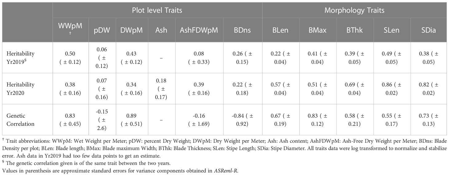
Table 1 Heritability across two years and genetic correlation between years for ten different traits.
Genetic correlation between dry weight per meter and morphology traits
The genetic correlation among traits was estimated within each year due to the large GxE for most traits. We used a multivariate model in the ASReml-R package (Butler et al., 2018). Due to model convergence issues, traits were analyzed in pairs and only for dry weight per meter and five individual morphological traits. An unstructured variance-covariance matrix across all traits was assumed in this model (Jia and Jannink, 2012; Fernandes et al., 2018):
Where Yi is the vector of phenotypic observations for the ith genotype: Yi = [Yi1 Yi2 … Yip ] , and p is the pth trait, μ = [μ1 μ2 … μp ], where is μp is the mean for the pth trait, and li , bi and ri are the line, block and year effects for the ith individual, respectively. The gi and ei terms are the genetic effects and residual effects for the ith individual, with gi = [gi1 gi2 … gip ] and ei= [ei1 ei2 … eip ]. Across all individuals, the vectorized genetic effects were distributed as g ~ Nnp(0,G0⊗G), where G0 is the among-trait genetic variance-covariance matrix and G is the additive relationship matrix. Similarly, e ~ Nnp(0,R0⊗I), where R0 is the among-trait residual variance-covariance matrix and I is an identity matrix showing our assumption that residuals are uncorrelated across plots (Fernandes et al., 2018).
Genomic prediction between diploid and haploid life stages
We obtained breeding values for all 866 SPs from Yr2019 and Yr2020, as well as the breeding values of their parental GPs, from the GBLUP model. This model takes into consideration the relatedness of individuals and hence GS predictive ability is higher for individuals that are more closely related to each other than if they are from separate populations (Windhausen et al., 2012). We only included phenotypic data from GOM to build GS models and did not use those from SNE for our GS analyses. Haploid GPs were selected to make crosses to create the confirmation population of diploid SPs grown in Yr2021. These GPs were used for crossing based on their available biomass (which determines the number of crosses to which they can contribute) and the following crossing design criteria: first, the GPs were ranked based on their dry weight per meter GEBVs. Parental GPs’ were then selected if their BVs were top ranked (n = 42), bottom ranked (n = 3), and randomly ranked (n = 25). In addition, we included GPs whose parental SPs were sampled from otherwise unrepresented locations (n = 5). Finally, we generated crosses that were repeats from the previous year (n = 12).
The GEBVs of Yr2021 diploid SPs were obtained as the sum of GEBVs from their parental female and male GPs, as estimated from equation (1), and their phenotypic observations were estimated using the Best Linear Unbiased Estimator (BLUEs), as explained below.
We assessed GS prediction accuracies as the correlation between BVs and BLUEs for all Yr2021 SPs (Table 3), for SPs within the category of parental GPs being top ranked, for SPs in the randomly selected category, and for SPs that were repeats from previous year (Supplemental Table 1). For the 12 common SPs between Yr2020 and Yr2021, we also estimated the phenotypic correlations between their within-year BLUEs. The analysis was done for each trait and prediction accuracy for all available traits that were recorded, even though selection of the Yr2021 population was only based on dry weight per meter.
Within-year cross validation genomic prediction accuracy
For modeling simplicity, GS model prediction accuracy comparisons were done with a two-step approach using the Yr2019 and Yr2020 data. The experimental block and line effects were statistically controlled for within each year to obtain BLUEs of SPs in ASReml-R. These BLUEs were then used as the response values to evaluate prediction accuracy under four different GS models using the BGLR package in R. The BLUEs were first estimated using the following model:
where Yijib is the ijlbth observation, μ is the overall mean, Gi is the ith genotype, Cj is the jth check group that distinguishes between experimental and check crosses, Ll is the lth line, and Bb is the bth block, and eijlbis the error associated with the ijlbth observation. The BLUEs for Yr2021 were estimated using the same model, but without a group effect Cj because none of the reference check plots generated high quality data.
Four GS models were run with a 10-fold cross validation scheme within each year. Each randomization scheme was repeated 20 times. The four models were:
A) General combining ability (GCA) and specific combining ability (SCA) using combined pedigree and marker relationship matrix
The mixed-ploidy combined pedigree and marker relationship matrix was used. General combining ability (GCA) and specific combining ability (SCA) components for the GP parents were included in the model with a formula adapted from Jarquin et al. (Jarquin et al., 2020):
where yi is the BLUE of the ith individual, gP1i and gP2i are the genetic effects of parent GP1 and parent GP2. And gP1i×P2i is the interaction effect of two parents, ei is the residual effect. The GCA and SCA account for the genetic main effects and the interaction effects, respectively, where the SCA variance-covariance matrix is the cell-wise product of the elements in variance-covariance matrix from parent 1 and from parent 2 (Jarquin et al., 2020).
For the purpose of estimating variance components and their 95% credible intervals (CIs), model (5) was also analyzed without cross validation (all data were used to predict BVs of all individuals). Variance components estimated were for female parent GCA (GCA_FG), male parent GCA (GCA_MG), SCA and error (varE). This model was run within each year and each running process was repeated 20 times. The lower- and upper- bound values of the 95% CI were averaged across the 20 replicates (Table 2).
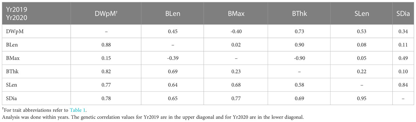
Table 2 Genetic correlation among traits using a multi-trait model in ASReml-R.
B) GCA+SCA model using only pedigree based relationship matrix
The same GCA +SCA model as formula (5) was used, except that the additive relationship matrix was estimated based only on pedigree. The GS 10-fold cross validation accuracies were obtained as in A.
C) Genomic Best Linear Unbiased Predictor (GBLUP) model using combined pedigree and markers relationship matrix
A basic GBLUP mixed model was used:
where X and Z is the design matrix for fixed effects β and for random effects u, respectively. ϵ is the error and u ~ , and G is the relationship matrix using combined pedigree and markers relationship matrix as estimated above. The 10-fold cross validation scheme being used was the same as the other models.
D) GBLUP model using only pedigree based relationship matrix
The same model as in formula (6) was used except that the G matrix was replaced by a relationship matrix estimated using pedigree information only.
Results
Population structure of GPs
Two clear subpopulations were revealed by PCA, separating GPs from GOM and SNE locations (Figure 1A) consistent with previous analyses of the founder SPs subpopulation structure (Mao et al., 2020). The remaining results and discussion pertain only to the GOM populations.

Figure 1 (A) Principal Component Analysis (PCA) for 276 GPs using 909,749 SNPs. Red symbols: Gulf of Maine (GOM), black symbols: Southern New England (SNE). (B) PCA for GPs within the GOM region. These gametophytes came from parents collected from the following locations: CB, Casco Bay farm (n= 28); CC, Cape Cod canal (n= 23); Check, gametophytes came from GOM checks crosses (n= 4); JS, Fort Stark (n= 22); LD, Lubec Dock (n= 27); LL, Lubec Light (n= 5); NC, New Castle (n= 19); NL, Nubble Light (n= 28); OD, Outer Dock (n= 11); OI, Orr’s Island (n= 32); and SF, Sullivan Falls (n= 14).
Heritability and genetic correlation between years
Trait heritabilities using two years’ data with the heterogeneous error model ranged from 0.06 to 0.86 (Table 1). Among six plot level (yield-related) traits, the highest heritability was for wet weight per meter in (0.50 in Yr2019), and lowest was for percent dry weight (0.06 in Yr2019). Among five morphology traits within each year, the highest heritability was for stipe length (0.86 in Yr2020), and the lowest was for blade length (0.22 in Yr2019, Table 1). All morphology traits had higher heritability in Yr2020 compared to Yr2019. In Yr2020, the heritabilities for morphology traits, measured at the individual blade level, were higher than plot-level yield-related traits (Table 1). The genetic correlation for all traits between the two years ranged from negative (ash related traits, percent dry weight and blade density) to strongly positive, with the highest being dry weight per meter (0.89 ± 0.51, Table 1). The heritability of ash free dry weight per meter was low one year (0.08, Yr2019), but higher the next year (0.39, Yr2020) while the between-year genetic correlation was nominally negative (-0.16 ± 1.7). The standard errors associated with between-year genetic correlation estimates were large, especially for traits with negative correlations, including percent dry weight (-0.15 ± 2.6) and blade density (-0.84 ± 0.92). None of the genetic correlations with nominally negative values were significantly different from zero. Lack of genotype by environment interaction results in a genetic correlation of 1 (Cooper and DeLacy, 1994). Even though the genetic correlations with negative nominal estimates were not significantly different from zero, they indicated large genotype by year interactions hence raising the possibility of more general genotype by environment interactions.
In the multivariate analysis to estimate genetic correlations between traits, we only included the results between dry weight per meter and the morphological traits due to model convergence problems. Given the genotype by environment interaction effects, the genetic correlation analysis was done within years. Dry weight per meter had higher genetic correlation with morphological traits in Yr2020 than in Yr2019. It was not genetically correlated with blade maximum width in either year (r = –0.40 in Yr2019 and r = 0.15 in Yr2020, Table 2). For individually measured morphological traits, blade length and blade thickness were strongly correlated in both years (r = 0.90 in Yr2019 and r = 0.69 in Yr2020, Table 2). Stipe length and stipe diameter had the highest consistent correlations in both years (r = 0.84 in Yr2019 and r = 0.95 in Yr2020, Table 2). Among-trait correlations of breeding values (BVs) averaged across two years showed that dry weight per meter was moderately correlated with most morphology traits (r = 0.47 for blade thickness to r = 0.58 for blade length), though it was uncorrelated with blade maximum width (r = –0.11, Figure 2). The correlation of blade density BV was relatively strongly correlated with wet and dry weight per meter (r = 0.55 and r = 0.54, respectively, Figure 2).
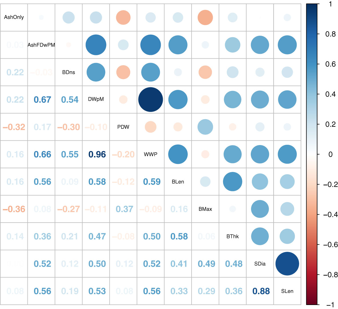
Figure 2 Correlation plot of SP breeding values estimated using both Yr2019 and Yr2020 data with the heterogeneous error variance GBLUP model. The combined BVs are the mean of estimates for Yr2019 and Yr2020.
Within-year cross validation genomic prediction accuracies
Genomic prediction accuracy with the GCA+SCA model using both pedigree and markers for all traits via 10-fold cross validation ranged from negative for percent dry weight, blade thickness to 0.48 for stipe length and stipe diameter (Table 3). For yield traits, the maximum prediction accuracy was for both wet weight and dry weight per meter (0.32 to 0.35, Table 3). Averaged across traits, prediction accuracy within Yr2020 was slightly lower numerically than within Yr2019 (Table 3). This lower accuracy also occurred across morphological traits despite their higher heritability in Yr2020 than Yr2019.
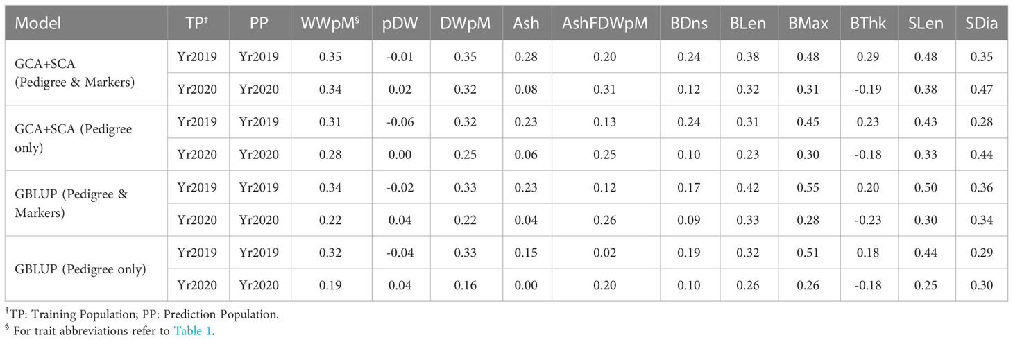
Table 3 Genomic prediction accuracy from 10-fold cross validation within each year. Each analysis was run with 20 replicates.
The GS cross validation accuracies from the GCA+SCA model using both pedigree and markers across all traits in two years was slightly higher (r = 0.27, averaged first two rows in Table 3) than that from the model of GCA+SCA with pedigree only (r = 0.22) and the base GBLUP model with pedigree and markers (r = 0.23) or GBLUP model with pedigree only (r = 0.20). While these differences were not significant for any single trait comparison, there was only one case (blade thickness in Yr2020) when prediction accuracy was higher without than with marker information (Table 3). The trend for GS within-year prediction accuracy was similar to that for heritability values across traits in that morphological traits tended to have higher GS prediction accuracy (and higher heritability) than yield-related traits (Tables 1, 3).
We compared the variance within each year due to female parents (GCA_FG) with those due to male parents (GCA_MG) using the MCMC-derived samples from the posterior distributions of these parameters. Across all yield-related and morphology traits, GCA_FG was greater than GCA_MG in 15 out of 22 trait-year combinations (Table 4). However, GCA_FG was significantly greater than GCA_MG only for stipe diameter in Yr2020, as determined by the fact that GCA_FG was greater than GCA_MG in over 97.5% of posterior samples (Table 4). Variance component results also explain the relative superiority of the GCA+SCA model over the base GBLUP model: in 17 out of 22 trait-year combinations the SCA variance component was greater than the average of the female and male GCA variance components (Table 4).
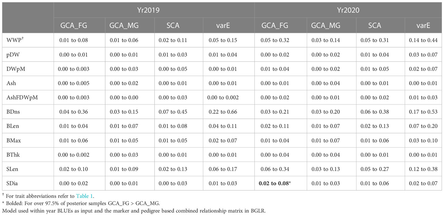
Table 4 The 95% credible interval of posterior distribution for variance components estimates: Variance due to GCA components from Female GPs (GCA_FG) and from Male GPs (GCA_MG), SCA component, and Error Variance (varE) based on the Variance component estimates.
Genomic prediction in both diploids and haploids
Due to the large genotype by environmental interactions and the differences in error variance observed between Yr2019 and Yr2020, we verified the ability of phenotypes from these years to predict performance in Yr2021. Our main interest was the BV for dry weight per meter (DWpM) trait for which we selected GPs to make crosses. GS prediction accuracy for Yr2021 SPs was defined as the correlation coefficient between trait BLUEs observed in 2021 and their predicted BVs, which were calculated as the sum of their parental FG and MG BVs. For the DWpM trait, GS accuracy for the 87 crosses in Yr2021 was r = 0.30 (using Yr2019 BVs) and r = 0.31 (using Yr2020 or combined BVs, Table 5). Over all other traits, GS accuracy ranged from negative (ash related traits, percent dry weight and blade density) to 0.80 (stipe length with Yr2019 GEBVs, Table 5). When heritability was high for a trait within a year, the prediction accuracy using that year’s data to predict Yr2021 also tended to be high (Tables 1, 5). Breeding values for founder SPs, GPs generated from founders, and SP progenies from those GPs all centered on zero (Figure 3). In contrast, GPs generated from SPs that were evaluated and selected on farms and SP progenies from those selected GPs deviated markedly from zero (Figure 3).
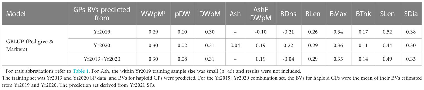
Table 5 Genomic prediction accuracy using heterogeneous error variance model, the same model as used in Table 1.
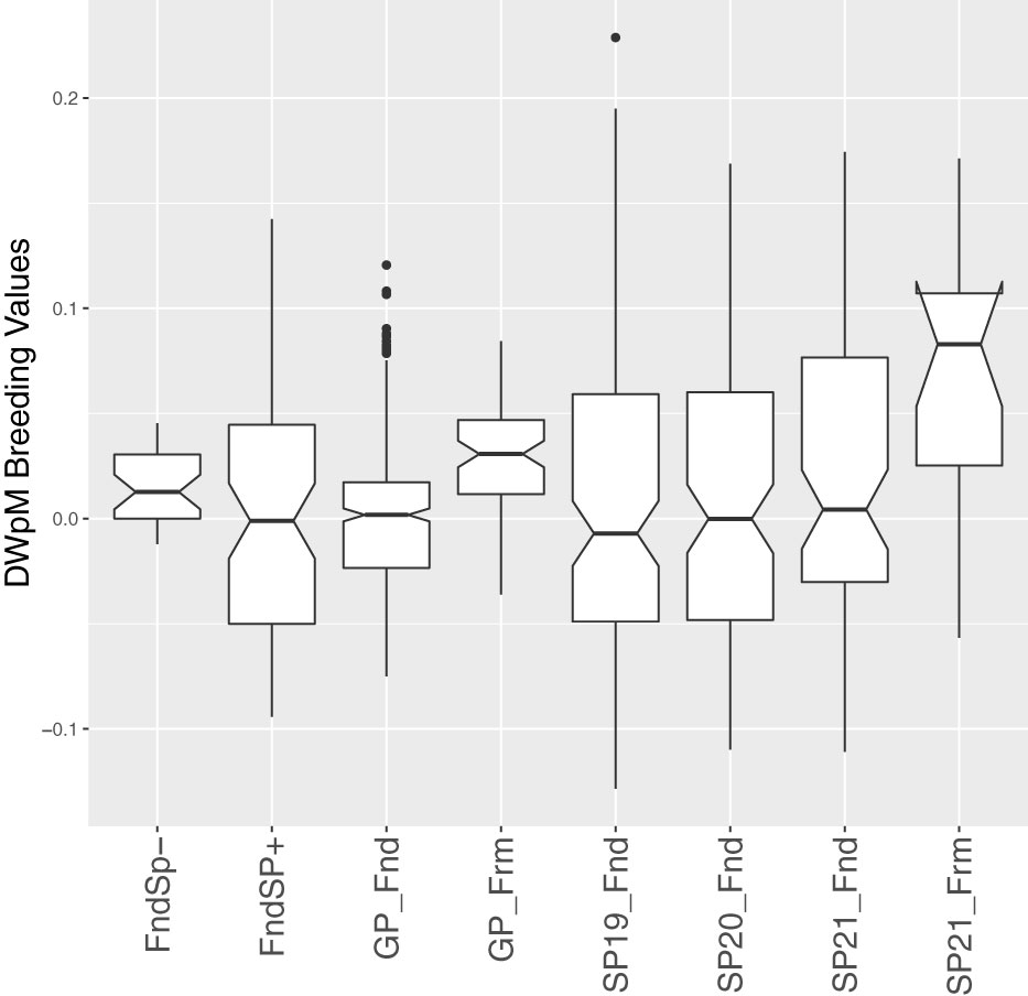
Figure 3 Box plots of estimated breeding values of DWpM (Dry Weight per Meter, log transformed) for 517 GPs and 436 SPs. The SPs included these subcategories: Founder SPs without progeny (these SPs were collected from the wild but did not produce GP progeny, denoted FndSP–), Founder SPs with progeny (FndSP+), SP19_Fnd (SPs tested on farm in Yr2019 generated using GPs from Founders), SP20_Fnd (SPs tested in Yr2020), SP21_Fnd (SPs tested in Yr2021), and SP21_Frm (SPs tested in Yr2021, generated using GPs collected from SPs tested on farm in Yr2019). The GPs included GPs collected from Founders (GP_Fnd) and GPs collected from SPs tested on farm in Yr2019 (GP_Frm).
Discussion
Population structure of GPs
Consistent with previous genetic analysis of the GOM founder SP populations (Mao et al., 2020), strong subpopulation structure was observed within the GPs from GOM region (Figure 1B) based on 909,749 SNP markers. A small but significant differentiation was observed between sampled locations by (Breton et al., 2017) for sugar kelp in Eastern Maine based on 12 microsatellite markers. Our SNP marker set analysis is an most up-to-date descriptor of GOM subpopulations.
Heritability, genetic correlation, and environmental variation
At this early stage in the development of technologies to breed, farm and phenotype diverse SP genotypes of sugar kelp, the heritabilities of yield-related traits are moderate to low (Table 1). The differences we observed in estimated heritability for the yield-related traits between years (Table 1) was likely due to changes in environmental conditions from one year to the next. The Yr2019 trial was planted later and harvested earlier than the Yr2020 trial, reducing total growth potential. Possibly as a result of these differing conditions, we found a negative genetic correlation between the two years for percent dry weight, ash related traits, and blade density, revealing high GxE and large year-to-year effects for these traits. Differences between years can also result from differences in nutrient availability which, in many nearshore sites, depends on runoff caused by rainfall events that vary annually (Grebe et al., 2021).
Phenotyping sugar kelp traits is challenging (Umanzor et al., 2021). Due to phenotyping limitations and labor constraints (all measurements were made on hundreds of crosses within 48 hours of harvest), we relied on subsampled data for blade density and percent dry weight to approximate whole plot traits. In theory each plot consists of uni-clonal individuals such that subsamples should be uniform. Yet, due to environmental and possible blade density effects, we observed non-uniform growth across the plot. Lack of uniformity among subsamples contributed to the error variance. To minimize the impact of this heterogeneity, we filtered data based on a visual score of plot uniformity (see Methods). We modified the measurement of dry weight related traits from Yr2019 to Yr2020. In Yr2019, percent dry weight was measured by a single value per plot where subsamples were combined and weighed together. In Yr2020, we measured the percent dry weight for the 10 largest blades out of the subsamples separately. Both approaches yielded low estimated heritability. This low heritability is in contrast to land crops where percent dry weight generally has high heritability (e.g., Rabbi et al., 2020) for root dry weight in cassava), though comparisons to traits in other domesticated species are perhaps unwarranted given the divergence, approximately 1,600 million years ago, of kelps from other eukaryotes (Hedges et al., 2004).
Because of the longer growing season in 2020 compared to 2019, dry weight per meter collected in 2020 were markedly higher than those in 2019. However, because connectivity between years came primarily from evaluating related SPs rather than from repeating evaluation of the same SPs across years, the genetic effects could also be partially confounded by year effects in the model.
Morphology traits were directly measured at the individual blade level, and we randomly measured 15 blades/plot in Yr2019. We modified the sampling procedure in Yr2020 by measuring only the longest ten blades from 3 subsamples within each plot. This modification ensured individual samples were more uniform within the same plot in Yr2020, likely reducing the error variance and leading to higher heritabilities for morphology traits in Yr2020 (Table 1). Blade length heritability more than doubled in the second year, and all other morphology traits also had increased heritability in Yr2020. In general, when traits had high heritability in both years, the genetic correlation values between years were also reasonable.
Multi-trait genetic correlation results among dry weight per meter and morphology traits indicated that genes underlying some of the morphology traits could play a role in contributing to kelp yield. Indeed, (Zhang et al., 2015) reported that QTLs clustered on the same chomosome region for morphological traits (frond length, width and thickness) as well as for yield related traits (raw weight) in a F2 mapping population created from a Saccharina longissima and Saccharina japonica parental combination. However, no genetic correlation among these traits was estimated (Zhang et al., 2015). The improved phenotyping protocol in Yr2020 could have contributed to a higher genetic correlation than those in Yr2019. Interestingly, stipe length and diameter were strongly correlated with each other in both years, indicating that they were controlled by the same group of genes across different environments (Egan et al., 1990).
Correlations from estimated BVs combined across two years on all plots revealed that dry weight per meter was correlated to other weight related traits except for percent dry weight (Figure 2). If a plot generates larger wet weight, it will also have a larger dry weight per meter and ash free dry weight per meter values (Figure 2). There was a clear correlation between plot level weights and blade density (r of 0.54 and 0.55 with dry and wet weight per meter, respectively, Figure 2). High blade density comes from the ability of the juvenile SP to attach to seed-string in the nursery, survive, and subsequently attach its holdfast to the farm grow-rope. This trait was not under selection in the wild, so it is not surprising that variation for this trait exists (Paaby and Rockman, 2014). Thus, blade density appears to be an important domestication trait.
The BVs of dry weight per meter were correlated to morphology traits, except blade maximum width (Figure 2). A similar pattern of positive genetic correlation was also observed in the multivariate analysis (Table 2). Previous studies reported that the multivariate model is favored as it allows borrowing information between traits and individuals across environments (Atanda et al., 2021). The multivariate genetic correlation results indicate that our selection for dry weight per meter could lead to morphologically longer and thicker blades, longer and larger stipes. The fact that wider blades were not particularly favored indicates that “skinny” individuals (designated Saccharina angustissima), originating from Casco Bay may have good adaptation to farms (Augyte et al., 2018). Indeed, (Li et al., 2022) showed that SPs with skinny kelp ancestry out-yielded SPs that had no skinny kelp ancestry. In our experiment, among the 42 Yr2021 top ranked SPs, 14 of them (33%) had a skinny kelp derived GP as a parent or grandparent. For comparison, of the 493 cross attempts made for Yr2019 and Yr2020 combined, 123 (25%) had a skinny kelp derived GP as a parent. A chi-square test showed these proportions were not significantly different.
Genomic prediction within years via cross validation
In previous studies, the GBLUP GS model produced similar accuracies across various traits compared to other GS models such as Bayesian approaches (Heslot et al., 2012; Sallam et al., 2015). Similarly, we did not observe significant differences between the model prediction accuracy of GBLUP (whether using pedigree alone, or using pedigree plus marker information) and GCA+SCA (whether using pedigree alone or using pedigree and marker information together). Nevertheless, for both GBLUP and GCA+SCA, addition of marker data improved prediction accuracy over pedigree information alone (Table 4). To our knowledge, we are the first to use the algorithm implemented in the CovCombR package (Akdemir et al., 2020) for an actual selection experiment. This approach allows the combination of data from different genotyping platforms without cross-platform imputation, therefore potentially simplifying the process. Our successful use of the method provides it with some validation.
While the prediction accuracy for GCA+SCA with pedigree and marker information was not significantly different from the other three models, it was numerically superior. There are two biological reasons why this model might be superior. First, we show suggestive evidence that the female contribution to trait expression is moderately more important than the male contribution. Prior studies have lacked sufficient numbers of crosses to assess this issue (Umanzor et al., 2021). Relevant mechanisms could be genomic imprinting (Reik and Walter, 2001; Yang et al., 2021) or simply the fact that the female GP plays a more important role in controlling kelp holdfast and stipe traits and, thus, attachment to the seed string and rope substrates (Garbary and South, 2013). Using the GCA+SCA with pedigree and marker model, we could distinguish between GCA variation contributed from the female versus male side. Across 22 comparisons (11 traits in each of two years, Table 4) the female contribution was significantly greater than the male contribution in only one case (Stipe Diameter in Yr2020, Table 4). However, the female contribution was numerically superior to the male contribution in 15 out of 22 cases when they were different (Table 4). A two-sided binomial test has a probability of 0.06 of that many cases occurring, though we note that the assumption of independence of the 22 cases is probably violated. While the GCA+SCA model allows the importance of parental contributions to differ, the standard GBLUP model forces them to be equal. Second, we also show evidence that the specific combining ability between the parental genomes is often important (Table 4): in 17 out of 22 cases, the SCA variance was greater than the mean of the two GCA variances. Again, given the lack of independence of these cases, we do not have a statistical test to conclusively show that SCA is greater than the GCAs, but this result does suggest it is biologically important. The SCA is caused by non-additive modes of gene action that the GBLUP model does not capture (Lynch and Walsh, 1998), therefore providing another mechanism making the GCA+SCA model superior to the GBLUP model.
GS accuracy estimates from cross validation are usually higher than estimates from independent datasets (Crossa et al., 2010; Michel et al., 2016; Huang et al., 2018). The GS accuracies for yield traits in previous studies varied from essentially zero to 0.75 (Zhao et al., 2012; Dawson et al., 2013; Fernandes et al., 2018; Stewart-Brown et al., 2019). The yield-related prediction accuracies via cross validation (r ranged from close to zero for ash free dry weight in the absence of marker data to 0.35 for wet weight with marker data, Table 3) fell within the range of those in previous studies in terrestrial crops (Zhao et al., 2012; Dawson et al., 2013; Michel et al., 2016; Stewart-Brown et al., 2019). We confirmed that GS prediction accuracy was related to trait heritability (Dawson et al., 2013; Lenz et al., 2020): in general, traits with high heritability gave good prediction accuracy, with an unexplained exception for blade thickness in Yr2020.
Genomic prediction between diploids and haploids
One of the biggest merits of applying genomic selection is that it can shorten the time per breeding cycle by directly predicting the breeding values of non-phenotyped individuals. In the case of sugar kelp breeding, the breeding germplasm is maintained in the form of GPs in culture. Because SP yield and composition traits cannot be obtained from GPs directly, genomic prediction is the only option for direct selection on those traits. The historical SP data from Yr2019 and Yr2020 was used to predict BVs of GPs, which were then used as parents for next generation SPs in Yr2021. The GS accuracy (r ~ 0.30) for dry weight per meter on the confirmation population was similar to the reports in other studies for grain yield (Zhao et al., 2012; Stewart-Brown et al., 2019). This reasonable prediction accuracy validated our method for calculating the pedigree-based mixed-ploidy relationship matrix and integrating it with marker-based genomic relationship matrices at the different ploidy levels. Simulations have shown that selection during both GP and SP phases of the kelp life cycle will generate the greatest breeding gain per unit time (Huang et al., 2022). This empirical research is the first to report that genomic prediction of haploid breeding values works. The use of GS in biphasic organisms, such as sugar kelp, can help breeders achieve higher efficiency in genetic gain.
The Yr2021 season was more similar to Yr2020 than Yr 2019 in terms of the overall length of the growing season and growth performance of the kelp plots. We were therefore somewhat surprised that Yr2019 and Yr2020 training data gave equal prediction accuracy of the Yr2021 validation data (Table 5). We show that, as for land crops (de Leon et al., 2016), genotype by year interaction is an important source of phenotypic variation (Table 1). Large GxE effects require a larger number of environments with repeated plots in order to properly evaluate genotype performance. Previous studies have confirmed that when more information is shared between environments or when sets of genotypes are observed across environments, the prediction accuracy can be increased (Jarquín et al., 2014; Lado et al., 2016; Jarquin et al., 2020). Future kelp breeding efforts need to take this source of variation into account.
Breeding value changes over generations of breeding cycles
Our empirical evaluations show some success in genomic selection: GPs derived from SPs that were evaluated on farm in Yr2019 (GP_Frm, Figure 3) were superior to GPs derived from founders (GP_Fnd, Figure 3) and, in turn, SPs derived from those GPs (SP21_Frm) were superior to SPs derived from founder GPs (SP19_Fnd, SP20_Fnd, and SP21_Fnd, Figure 3). We note that the superiority of farm-derived GPs occurred despite minimal selection pressure on the SP parents of those GPs (Supp. Figure 1). Improvements in our experimental procedures meant that we collected twice as many SPs that had successful spore release in Yr2020 (Supp. Figure 1, green dashed lines) than in Yr2019 (red dashed lines). This improvement was mainly due to the fact that more plots in Yr2020 than Yr2019 were mature (longer growing season) and hence more plots produced sorus tissue. The Yr2020 plots also had a larger proportion of SPs that were top ranked compared to Yr2019 (Supp. Figure 1). Greater success in releasing and isolating numerous individual spores from select harvested mature SPs (or artificially inducing maturity) will lead to higher selection intensity in both the SP and GP phases (Huang et al., 2022). The response of GPs despite low selection pressure (number of mature and good performing individuals to propogate the next generation) in Yr2019 (Figure 3) suggests that, in addition to artificial selection, some amount of natural selection is also taking place within our breeding program as we prompt kelp that are naturally adapted to attaching to rock substrates to being adapted to the seed string and rope substrates. Continued selection in this way may lead to appreciably “domesticated” kelp in the sense that our germplasm may be better adapted to the off-shore farm environment than to the natural rocky nearshore habitat.
Future research areas
The use of a pedigree and marker estimated relationship matrix between lab-grown GP cultures and the field-grown SPs enabled us to predict breeding values of the GPs and to select the top ranking ones to make new crosses. Our results indicate that progress can be made in sugar kelp breeding by genomic selection, especially for dry weight per meter. To the best of our knowledge, our study is the first to evaluate the use of GS in kelp breeding, including a mixed-ploidy relationship matrix and the integration of separate genomic relationship matrices at the two ploidy levels. Our findings are applicable for other bi- and tri phasic algae such as Gracilaria spp. (Gupta et al., 2011) and Asparagopsis spp. (Roque et al., 2021). Researchers could first train a GS model using individuals with known phenotypic data and genotypic data. Then use the model to predict breeding values for the individuals at a life stage that is hard to be phenotyped. These predicted individuals have to be genotyped and ideally should be related to individuals in the training model. This allows selection on the phase that was not possible previously without the GS tool. Our results specifically show that wet weight and dry weight per meter can be effectively selected via GS. However, continued efforts in improving nursery/planting and phenotyping methods, as well as increasing the number of plots to be evaluated on farms will be critical for us to continuously improve prediction accuracy. The GS model should also be updated and retrained as we move forward using data from related individuals. The low across-year genetic correlations we observed were concerning (Table 1). These findings need to be backed up with further experimentations, including the addition of common individuals across environments. Finally, our results with the GCA+SCA model suggest that it may be superior to the standard GBLUP model for kelp genomic predictions, but validation of that hypothesis will require more experimental data.
Data availability statement
The datasets presented in this study can be found in online repositories. The names of the repository/repositories and accession number(s) can be found in the article/Supplementary Material.
Author contributions
MH performed the analyses, wrote the manuscript draft, and revised the manuscript together with other coauthors. KR and J-LJ guided the analyses. J-LJ contributed to analysis scripts. YL, SU, SL, and CY edited the manuscript. MH, YL, SU, MM-R, CY, DB, MA, and SL collected phenotypic data. JS and JG performed DNA extraction and sequencing. SL, CY, and J-LJ led the project. All authors contributed to the article and approved the submitted version.
Funding
We acknowledge funding support from the U.S. Department of Energy ARPA-E (DE-AR0000915), and the Massachusetts Clean Energy Center (AmplifyMass).
Acknowledgments
We thank Jeff Glaubitz from Cornell Institute of Biotechnology for consultation on bioinformatics. This work has been published as a reprint in bioRxiv (2022.08.01.502376).
Conflict of interest
The authors declare that the research was conducted in the absence of any commercial or financial relationships that could be construed as a potential conflict of interest.
Publisher’s note
All claims expressed in this article are solely those of the authors and do not necessarily represent those of their affiliated organizations, or those of the publisher, the editors and the reviewers. Any product that may be evaluated in this article, or claim that may be made by its manufacturer, is not guaranteed or endorsed by the publisher.
Supplementary material
The Supplementary Material for this article can be found online at: https://www.frontiersin.org/articles/10.3389/fmars.2023.1040979/full#supplementary-material
References
Akdemir D., Knox R., Isidro Y Sánchez J. (2020). Combining partially overlapping multi-omics data in databases using relationship matrices. Front. Plant Sci. 11, 947. doi: 10.3389/fpls.2020.00947
Asoro F. G., Newell M. A., Beavis W. D., Scott M. P., Jannink J.-L. (2011). Accuracy and training population design for genomic selection on quantitative traits in elite north American oats. Plant Genome 4, 132–144. doi: 10.3835/plantgenome2011.02.0007
Atanda S. A., Olsen M., Crossa J., Burgueño J., Rincent R., Dzidzienyo D., et al. (2021). Scalable sparse testing genomic selection strategy for early yield testing stage. Front. Plant Sci. 12, 658978. doi: 10.3389/fpls.2021.658978
Augyte S., Lewis L., Lin S., Neefus C. D., Yarish C. (2018). Speciation in the exposed intertidal zone: The case of saccharina angustissima comb. nov. & stat. nov. (Laminariales, phaeophyceae). Phycologia 57 (1), 100–112. doi: 10.2216/17-40.1
Augyte S., Yarish C., Redmond S., Kim J. K. (2017). Cultivation of a morphologically distinct strain of the sugar kelp, saccharina latissima forma angustissima, from coastal Maine, USA, with implications for ecosystem services. J. Appl. Phycol. 29, 1967–1976. doi: 10.1007/s10811-017-1102-x
Breton T. S., Nettleton J. C., O’Connell B., Bertocci M. (2017). Fine-scale population genetic structure of sugar kelp, saccharina latissima (Laminariales, phaeophyceae), in eastern Maine, USA. Phycologia 57, 32–40. doi: 10.2216/17-72.1
Brito F. V., Neto J. B., Sargolzaei M., Cobuci J. A., Schenkel F. S. (2011). Accuracy of genomic selection in simulated populations mimicking the extent of linkage disequilibrium in beef cattle. BMC Genet. 12, 80. doi: 10.1186/1471-2156-12-80
Bruhn A., Brynning G., Johansen A., Lindegaard M. S., Sveigaard H. H., Aarup B., et al. (2019). Fermentation of sugar kelp (Saccharina latissima)–effects on sensory properties, and content of minerals and metals. J. Appl. Phycol. 31, 3175–3187. doi: 10.1007/s10811-019-01827-4
Butler D. G., Cullis B. R., Gilmour A. R., Gogel B. G., Thompson R. (2018). ASReml-R Reference Manual Version 4 ASReml estimates variance components under a general linear mixed model by residual maximum likelihood (REML). (Hemel hempstead: VSN international Ltd.).
Clark S., Hickey J. M., Daetwyler H. D., van der Werf J. H. J. (2012). The importance of information on relatives for the prediction of genomic breeding values and the implications for the makeup of reference data sets in livestock breeding schemes. Genet. Sel. Evol. 44, 4–4. doi: 10.1186/1297-9686-44-4
Cooper M., DeLacy I. H. (1994). Relationships among analytical methods used to study genotypic variation and genotype-by-environment interaction in plant breeding multi-environment experiments. Theor. Appl. Genet. 88, 561–572. doi: 10.1007/BF01240919
Crossa J., Campos G. D. L., Pérez P., Gianola D., Burgueño J., Araus J. L., et al. (2010). Prediction of genetic values of quantitative traits in plant breeding using pedigree and molecular markers. Genetics 186, 713–724. doi: 10.1534/genetics.110.118521
Danecek P., Auton A., Abecasis G., Albers C. A., Banks E., DePristo M. A., et al. (2011). The variant call format and VCFtools. Bioinformatics 27, 2156–2158. doi: 10.1093/bioinformatics/btr330
Dawson J. C., Endelman J. B., Heslot N., Crossa J., Poland J., Dreisigacker S., et al. (2013). The use of unbalanced historical data for genomic selection in an international wheat breeding program. Field Crops Res. 154, 12–22. doi: 10.1016/j.fcr.2013.07.020
de Leon N., Jannink J.-L., Edwards J. W., Kaeppler S. M. (2016). Introduction to a special issue on genotype by environment interaction. Crop Sci. 56, 2081–2089. doi: 10.2135/cropsci2016.07.0002in
Deng C., Lin R., Kang X., Wu B., O’Shea R., Murphy J. D. (2020). Improving gaseous biofuel yield from seaweed through a cascading circular bioenergy system integrating anaerobic digestion and pyrolysis. Renewable Sustain. Energy Rev. 128, 109895. doi: 10.1016/j.rser.2020.109895
Duran-Frontera E. (2017)Development of a process approach for retaining seaweed sugar kelp (Saccharina latissima) nutrients. Available at: https://digitalcommons.library.umaine.edu/honors/297/ (Accessed Jan-03, 2022).
Egan B., Garcia-Ezquivel Z., Brinkhuis B. H., Yarish C. (1990). “Genetics of morphology and growth in laminaria from the north Atlantic ocean — implications for biogeography,” in Evolutionary biogeography of the marine algae of the north Atlantic (Springer-Verlag, Berlin, Germany:Springer Berlin Heidelberg), 147–171.
Emik L. O., Terrill C. E. (1949). Systematic procedures for calculating inbreeding coefficients. J. Hered. 40, 51–55. doi: 10.1093/oxfordjournals.jhered.a105986
Endelman J. B. (2011). Ridge regression and other kernels for genomic selection with r package rrBLUP. Plant Genome J. 4, 250–250. doi: 10.3835/plantgenome2011.08.0024
Endelman J. B., Jannink J.-L. (2012). Shrinkage estimation of the realized relationship matrix. G3: Genes|Genomes|Genetics 2, 1405–1413. doi: 10.1534/g3.112.004259
Fernandes S. B., Dias K. O. G., Ferreira D. F., Brown P. J. (2018). Efficiency of multi-trait, indirect, and trait-assisted genomic selection for improvement of biomass sorghum. Theor. Appl. Genet. 131, 747–755. doi: 10.1007/s00122-017-3033-y
Garbary D. J., South G. R. (2013). Evolutionary biogeography of the marine algae of the north atlantic. Berlin, Germany. Springer-Verlag 429.
Grebe G. S., Byron C. J., Brady D. C., Geisser A. H., Brennan K. D. (2021). The nitrogen bioextraction potential of nearshore saccharina latissima cultivation and harvest in the Western gulf of Maine. J. Appl. Phycol. 33, 1741–1757. doi: 10.1007/s10811-021-02367-6
Gupta V., Baghel R. S., Kumar M., Kumari P., Mantri V. A., Reddy C. R. K., et al. (2011). Growth and agarose characteristics of isomorphic gametophyte (male and female) and sporophyte of gracilaria dura and their marker assisted selection. Aquaculture 318, 389–396. doi: 10.1016/j.aquaculture.2011.06.009
Guzinski J., Mauger S., Cock J. M., Valero M. (2016). Characterization of newly developed expressed sequence tag-derived microsatellite markers revealed low genetic diversity within and low connectivity between European saccharina latissima populations. J. Appl. Phycol. 28, 3057–3070. doi: 10.1007/s10811-016-0806-7
Guzinski J., Ruggeri P., Ballenghien M., Mauger S., Jacquemin B., Jollivet C., et al. (2020). Seascape genomics of the sugar kelp saccharina latissima along the north Eastern Atlantic latitudinal gradient. Genes 11, 1503. doi: 10.3390/genes11121503
Hedges S. B., Blair J. E., Venturi M. L., Shoe J. L. (2004). A molecular timescale of eukaryote evolution and the rise of complex multicellular life. BMC Evol. Biol. 4, 2. doi: 10.1186/1471-2148-4-2
Heslot N., Yang H.-P., Sorrells M. E., Jannink J.-L. (2012). Genomic selection in plant breeding: A comparison of models. Crop Sci. 52, 146–160. doi: 10.2135/cropsci2011.06.0297
Huang M., Balimponya E. G., Mgonja E. M., McHale L. K. (2019). Use of genomic selection in breeding rice (Oryza sativa l.) for resistance to rice blast (Magnaporthe oryzae). Mol. Breed. 39, 114. doi: 10.1007/s11032-019-1023-2
Huang M., Cabrera A., Hoffstetter A., Griffey C., Van Sanford D., Costa J., et al. (2016). Genomic selection for wheat traits and trait stability. Theor. Appl. Genet. 129, 1697–1710. doi: 10.1007/s00122-016-2733-z
Huang M., Robbins K. R., Li Y., Umanzor S., Marty-Rivera M., Bailey D., et al. (2022). Simulation of sugar kelp (Saccharina latissima) breeding guided by practices to accelerate genetic gains. G3 12 (3), jkac003. doi: 10.1093/g3journal/jkac003
Huang M., Ward B., Griffey C., Van Sanford D. (2018). The accuracy of genomic prediction between environments and populations for soft wheat traits. Crop Sci. 58 (6), 2274. doi: 10.2135/cropsci2017.10.0638
Jannink J.-L., Lorenz A. J., Iwata H. (2010). Genomic selection in plant breeding: from theory to practice. Brief. Funct. Genomics 9, 166–177. doi: 10.1093/bfgp/elq001
Jarquín D., Crossa J., Lacaze X., Du Cheyron P., Daucourt J., Lorgeou J., et al. (2014). A reaction norm model for genomic selection using high-dimensional genomic and environmental data. Theor. Appl. Genet. 127, 595–607. doi: 10.1007/s00122-013-2243-1
Jarquin D., Howard R., Liang Z., Gupta S. K., Schnable J. C., Crossa J. (2020). Enhancing hybrid prediction in pearl millet using genomic and/or multi-environment phenotypic information of inbreds. Front. Genet. 10, 1294. doi: 10.3389/fgene.2019.01294
Jia Y., Jannink J.-L. (2012). Multiple trait genomic selection methods increase genetic value prediction accuracy. Genetics 192 (4), 1513–1522. doi: 10.1534/genetics.112.144246
Kerrison P. D., Stanley M. S., Edwards M. D., Black K. D., Hughes A. D. (2015). The cultivation of European kelp for bioenergy: Site and species selection. Biomass Bioenergy 80, 229–242. doi: 10.1016/j.biombioe.2015.04.035
Kim J. K., Kraemer G. P., Yarish C. (2015)Use of sugar kelp aquaculture in long island sound and the Bronx river estuary for nutrient extraction. Available at: https://www.int-res.com/abstracts/meps/v531/p155-166/ (Accessed Jan-03-2023).
Kim J., Stekoll M., Yarish C. (2019). Opportunities, challenges and future directions of open-water seaweed aquaculture in the united states. Phycologia 58, 446–461. doi: 10.1080/00318884.2019.1625611
Kim J. K., Yarish C., Hwang E. K., Park M., Kim Y., Kim J. K. (2017). Seaweed aquaculture: cultivation technologies, challenges and its ecosystem services. Algae 32 (1), 1–3. doi: 10.4490/algae.2017.32.3.3
Kirkholt E. M., Dikiy A., Shumilina E. (2019). Changes in the composition of Atlantic salmon upon the brown seaweed (Saccharina latissima) treatment. Foods 8, (12), 625. doi: 10.3390/foods8120625
Lado B., Barrios P. G., Quincke M., Silva P., Gutiérrez L. (2016). Modeling genotype × environment interaction for genomic selection with unbalanced data from a wheat breeding program. Crop Sci. 56, 2165–2179. doi: 10.2135/cropsci2015.04.0207
Lenz P. R. N., Nadeau S., Azaiez A., Gérardi S., Deslauriers M., Perron M., et al. (2020). Genomic prediction for hastening and improving efficiency of forward selection in conifer polycross mating designs: an example from white spruce. Heredity 124, 562–578. doi: 10.1038/s41437-019-0290-3
Li H. (2011). Improving SNP discovery by base alignment quality. Bioinformatics 27, 1157–1158. doi: 10.1093/bioinformatics/btr076
Li H., Durbin R. (2010). Fast and accurate long-read alignment with burrows–wheeler transform. Bioinformatics 26, 589–595. doi: 10.1093/bioinformatics/btp698
Li H., Handsaker B., Wysoker A., Fennell T., Ruan J., Homer N., et al. (2009). The sequence Alignment/Map format and SAMtools. Bioinformatics 25, 2078–2079. doi: 10.1093/bioinformatics/btp352
Li Y., Umanzor S., Ng C., Huang M., Marty-Rivera M., Bailey D., et al. (2022). Skinny kelp (Saccharina angustissima) provides valuable genetics for the biomass improvement of farmed sugar kelp (Saccharina latissima). J. Appl. Phycol. 34, 2551–2563. doi: 10.1007/s10811-022-02811-1
Lüning K., Mortensen L. (2015). European Aquaculture of sugar kelp (Saccharina latissima) for food industries: iodine content and epiphytic animals as major problems. Botanica Marina 58, 449–455. doi: 10.1515/bot-2015-0036
Luttikhuizen P. C., van den Heuvel F. H. M., Rebours C., Witte H. J., van Bleijswijk J. D. L., Timmermans K. (2018). Strong population structure but no equilibrium yet: Genetic connectivity and phylogeography in the kelp saccharina latissima (Laminariales, phaeophyta). Ecol. Evol. 8, 4265–4277. doi: 10.1002/ece3.3968
Lynch M., Walsh B. (1998). Genetics and analysis of quantitative traits (Sunderland, MA: Sinauer Associates).
Mao X., Augyte S., Huang M., Hare M. P., Bailey D., Umanzor S., et al. (2020). Population genetics of sugar kelp throughout the northeastern united states using genome-wide markers. Front. Mar. Sci. 7, 694. doi: 10.3389/fmars.2020.00694
Marinho G. S., Holdt S. L., Birkeland M. J., Angelidaki I. (2015). Commercial cultivation and bioremediation potential of sugar kelp, saccharina latissima, in Danish waters. J. Appl. Phycol. 27, 1963–1973. doi: 10.1007/s10811-014-0519-8
Meuwissen T. H. E., Hayes B. J., Goddard M. E. (2001). Prediction of total genetic value using genome-wide dense marker maps. Genetics 157, 1819–1829. doi: 10.1093/genetics/157.4.1819
Michel S., Ametz C., Gungor H., Epure D., Grausgruber H., Löschenberger F., et al. (2016). Genomic selection across multiple breeding cycles in applied bread wheat breeding. Theor. Appl. Genet. 129, 1179–1189. doi: 10.1007/s00122-016-2694-2
Paaby A. B., Rockman M. V. (2014). Cryptic genetic variation: evolution’s hidden substrate. Nat. Rev. Genet. 15, 247–258. doi: 10.1038/nrg3688
Peteiro C., Sánchez N., Martínez B. (2016). Mariculture of the Asian kelp undaria pinnatifida and the native kelp saccharina latissima along the Atlantic coast of southern Europe: An overview. Algal Res. 15, 9–23. doi: 10.1016/j.algal.2016.01.012
Rabbi I. Y., Kayondo S. I., Bauchet G., Yusuf M., Aghogho C. I., Ogunpaimo K., et al. (2020). Genome-wide association analysis reveals new insights into the genetic architecture of defensive, agro-morphological and quality-related traits in cassava. Plant Mol. Biol. 109, 195–213. doi: 10.1007/s11103-020-01038-3
Rabier C.-E., Barre P., Asp T., Charmet G., Mangin B. (2016). On the accuracy of genomic selection. PloS One 11, e0156086. doi: 10.1371/journal.pone.0156086
R Core Team (2022)R: A language and environment for statistical computing. Available at: https://www.R-project.org/ (Accessed Jan-03-2023).
Reik W., Walter J. (2001). Genomic imprinting: Parental influence on the genome. Nat. Rev. Genet. 2, 21–32. doi: 10.1038/35047554
Resende M. F. R. C.OMMAJ.R.X.X.X, Del Valle P. R. M., Acosta J. J., Resende M. D. V., Grattapaglia D., Kirst M. (2011). Stability of genomic selection prediction models across ages and environments. BMC Proc. 5, O14. doi: 10.1186/1753-6561-5-S7-O14
Rey F., Lopes D., Maciel E., Monteiro J., Skjermo J., Funderud J., et al. (2019). Polar lipid profile of saccharina latissima, a functional food from the sea. Algal Res. 39, 101473. doi: 10.1016/j.algal.2019.101473
Roque B. M., Venegas M., Kinley R. D., de Nys R., Duarte T. L., Yang X., et al. (2021). Red seaweed (Asparagopsis taxiformis) supplementation reduces enteric methane by over 80 percent in beef steers. PloS One 16, e0247820. doi: 10.1371/journal.pone.0247820
Rutkoski J., Singh R. P., Huerta-Espino J., Bhavani S., Poland J., Jannink J.-L., et al. (2015). Genetic gain from phenotypic and genomic selection for quantitative resistance to stem rust of wheat. Plant Genome 8, 1–10. doi: 10.3835/plantgenome2014.10.0074
Sallam A. H., Endelman J. B., Jannink J.-L., Smith K. P. (2015). Assessing genomic selection prediction accuracy in a dynamic barley breeding population. Plant Genome 8, 1–15. doi: 10.3835/plantgenome2014.05.0020
Sappati P. K., Nayak B., VanWalsum G. P., Mulrey O. T. (2019). Combined effects of seasonal variation and drying methods on the physicochemical properties and antioxidant activity of sugar kelp (Saccharina latissima). J. Appl. Phycol. 31, 1311–1332. doi: 10.1007/s10811-018-1596-x
Stewart-Brown B. B., Song Q., Vaughn J. N., Li Z. (2019). Genomic selection for yield and seed composition traits within an applied soybean breeding program. G3 9, 2253–2265. doi: 10.1534/g3.118.200917
Thornber C. S. (2006). Functional properties of the isomorphic biphasic algal life cycle. Integr. Comp. Biol. 46, 605–614. doi: 10.1093/icb/icl018
Umanzor S., Li Y., Bailey D., Augyte S., Huang M., Marty-Rivera M., et al. (2021). Comparative analysis of morphometric traits of farmed sugar kelp and skinny kelp, saccharina spp., strains from the Northwest Atlantic. J. World Aquac. Soc. 52 (5), 1059–1068.doi: 10.1111/jwas.12783
van den Burg S., Selnes T., Alves L., Giesbers E., Daniel A. (2021). Prospects for upgrading by the European kelp sector. J. Appl. Phycol. 33, 557–566. doi: 10.1007/s10811-020-02320-z
Vijn S., Compart D. P., Dutta N., Foukis A., Hess M., Hristov A. N., et al. (2020). Key considerations for the use of seaweed to reduce enteric methane emissions from cattle. Front. Vet. Sci. 7, 597430. doi: 10.3389/fvets.2020.597430
Vincent A., Stanley A., Ring J. (2020)Hidden champion of the ocean: Seaweed as a growth engine for a sustainable European future. Available at: https://www.seaweedeurope.com/wp-content/uploads/2020/10/Seaweed_for_Europe-Hidden_Champion_of_the_ocean-Report.pdf (Accessed Jan-03-2023).
Windhausen V. S., Atlin G. N., Hickey J. M., Crossa J., Jannink J.-L., et al. (2012). Effectiveness of genomic prediction of maize hybrid performance in different breeding populations and environments. G3: Genes Genomes Genet. 2 (11), 1427–1436. doi: 10.1534/g3.112.003699
Yang X., Wang X., Yao J., Duan D. (2021). Genome-wide mapping of cytosine methylation revealed dynamic DNA methylation patterns associated with sporophyte development of saccharina japonica. Int. J. Mol. Sci. 22 (18), 9877. doi: 10.3390/ijms22189877
Yarish C., Kim J. K., Lindell S., Kite-Powell H. (2017)Developing an environmentally and economically sustainable sugar kelp aquaculture industry in southern new England: From seed to market. Available at: https://opencommons.uconn.edu/eeb_articles/38/ (Accessed Jan-03-2023).
Zhang J., Liu T., Feng R., Liu C., Chi S. (2015). Genetic map construction and quantitative trait locus (QTL) detection of six economic traits using an F2 population of the hybrid from saccharina longissima and saccharina japonica. PloS One 10, e0128588. doi: 10.1371/journal.pone.0128588
Zhao Y., Gowda M., Liu W., Würschum T., Maurer H. P., Longin F. H., et al. (2012). Accuracy of genomic selection in European maize elite breeding populations. Theor. Appl. Genet. 124, 769–776. doi: 10.1007/s00122-011-1745-y
Keywords: sugar kelp (Saccharina latissima), genomic selection (GS), genotyping, phenotyping, brown algae, biphasic cycle, breeding
Citation: Huang M, Robbins KR, Li Y, Umanzor S, Marty-Rivera M, Bailey D, Aydlett M, Schmutz J, Grimwood J, Yarish C, Lindell S and Jannink J-L (2023) Genomic selection in algae with biphasic lifecycles: A Saccharina latissima (sugar kelp) case study. Front. Mar. Sci. 10:1040979. doi: 10.3389/fmars.2023.1040979
Received: 09 September 2022; Accepted: 09 January 2023;
Published: 22 February 2023.
Edited by:
Carmen Navarro-Guillén, Spanish National Research Council (CSIC), SpainReviewed by:
Paolo Ruggeri, Xelect, Ltd., United KingdomQian Lu, Jiangsu University of Science and Technology, China
Copyright © 2023 Huang, Robbins, Li, Umanzor, Marty-Rivera, Bailey, Aydlett, Schmutz, Grimwood, Yarish, Lindell and Jannink. This is an open-access article distributed under the terms of the Creative Commons Attribution License (CC BY). The use, distribution or reproduction in other forums is permitted, provided the original author(s) and the copyright owner(s) are credited and that the original publication in this journal is cited, in accordance with accepted academic practice. No use, distribution or reproduction is permitted which does not comply with these terms.
*Correspondence: Jean-Luc Jannink, amVhbmx1Yy5qYW5uaW5rQHVzZGEuZ292