 Xiying Sun
 Zhaohui Chen
 Chao Zhang1,5
95% of researchers rate our articles as excellent or good
Learn more about the work of our research integrity team to safeguard the quality of each article we publish.
Find out more
ORIGINAL RESEARCH article
Front. Mar. Sci. , 25 January 2023
Sec. Marine Biogeochemistry
Volume 10 - 2023 | https://doi.org/10.3389/fmars.2023.1027710
This article is part of the Research Topic Biogeochemical, Ecological and Biophysical Dynamics in the Kuroshio, Oyashio and Their Extension Regions View all 17 articles
The bimodal and unimodal seasonal cycles of surface Chlorophyll-a (Chl-a) concentration (SCC) are ubiquitous in the mid-latitude oceans. The nutrient and light are regarded as two key factors affecting such seasonal differences. However, our quantitative knowledge of distinguishing these two factors is still inadequate in mid-latitude regions where they limit primary productivity simultaneously. It hinders the full understanding of the underlying mechanisms of seasonal blooms. In this study, the bimodal and unimodal variations of SCC in the Kuroshio Extension (KE) region have been investigated, with a special focus on the emergence latitudes of the secondary peak, i.e., the phytoplankton fall bloom. Based on satellite observations, we have found that the SCC bloom emerges in spring and fall in the northern region, and that spring (fall) bloom starts later (earlier) as the latitude gets higher. In the southern part of KE, by contrast, the SCC tends to peak in late winter or early spring with its bloom time delaying gradually with increasing latitude. A regression model regarding the role of the nutrient and light has been proposed to reconstruct the seasonal variations of the observed SCC, and the relative contributions of the two factors have been assessed quantitatively. It is shown that the regression model has reasonably captured the seasonal variations of SCC in terms of the bimodal/unimodal feature as well as the time of occurrence. Specifically, we have found the boundary between bimodality and unimodality areas moves northward as KE flows eastward, which corresponds to the equivalent contribution of the nutrient and light to the SCC variation and the eastward-decreasing nutrient at the same latitude. Moreover, we have used the model to explore the lag effect of light on regulating the seasonal cycle of SCC, which is associated with the light-heating process, the resultant ocean vertical stratification and the nutrient deficiency, the time interval between the growth rate and SCC, as well as light attenuation within the mixed layer. In the context of global warming, our study has provided insights into the switch pattern between bimodality and unimodality of SCC in mid-latitude oceans.
The Northwest Pacific (NWP) is the most productive area characterized by high primary productivity (PP) and active fishing grounds with the highest fishery production in the world (Kim, 2010; Yatsu and Ye, 2011), among which the Kuroshio Extension (KE) and its adjacent regions are regarded as a “hotspot” of PP with significant carbon sinks (Ogawa et al., 2006; Takahashi et al., 2009; Fassbender et al., 2017). Meanwhile, it is one of the most dynamical regions full of varying oceanic processes and air-sea interactions in multi-temporal and spatial scales (Qiu, 2003; Taguchi et al., 2009; Xie et al., 2011; Jing et al., 2020; Joh et al., 2021; Yang et al., 2021), which exerts an important effect on PP and the process of carbon export (Takamura et al., 2010; Fassbender et al., 2017). Chlorophyll-a (Chl-a), as an important indicator of phytoplankton biomass, can reflect the production levels to a large extent (Antoine et al., 1996). The temporal and spatial variability of surface Chl-a concentration (SCC), therefore, acts as an important agent to estimate and predict the carbon fixation and associated export process in this special region.
The KE region spans from subtropical to subpolar gyres of the NWP, leading to the pronounced variations in SCC from sub-seasonal to seasonal scales as revealed by the decade-long accumulation of satellite-oriented ocean color data. The SCC at lower latitudes of the KE region generally only peaks in late winter or early spring (i.e., SCC unimodality, Yoo et al., 2008), which is predominantly determined by nutrient availability. At higher latitudes, the combined effect of the nutrient and light leads to the spring and fall blooms of SCC (i.e., SCC bimodality, Kim et al., 2007; Yoo et al., 2008; Matsumoto et al., 2014; Yu et al., 2019). The diagram of seasonal change in the nutrient and light availability has been schematically described to shape the unimodality/bimodality of SCC (Lalli and Parsons, 2004), but our knowledge of their transition latitudes and the quantitative role of the nutrient and light in this specific region is fragmented. Moreover, although numerous studies have explored the relationship between phytoplankton growth and nutrient and/or light availability at species and community levels, it is still difficult to extrapolate these theories and equations to large-scale oceans, where various factors, e.g., the lag effect of light on sea water temperature and isopycnal heaving induced by upwellings, can affect the large-scale responses of phytoplankton (Bindloss, 1976; Le et al., 2022).
Apart from the unimodality/bimodality of SCC in the KE region, the magnitudes and time of fall blooms at higher latitudes are of vital ecological impact, mainly impacting fisheries (Zhang et al., 2000; Friedland et al., 2009) and biogeochemical cycles (Honda and Watanabe, 2010). For lack of knowledge on the quantitative contributions of environmental factors, it is also difficult to explain the emergence latitudes of the fall bloom, as well as the misalignment with the transition zone Chl-a front defined as 0.2 mg/m3 SCC (Polovina et al., 2001), as shown in Figure 1. With the ongoing global warming, the seasonal cycles of SCC and PP in the KE region may be inevitably influenced by the changing environmental backgrounds, such as the shifting of the KE axis and the strengthening of upper ocean stratification (Coma et al., 2009). In this regard, it is necessary to figure out the combined effects of nutrient and light in a quantitative way to better predict the future responses of SCC and the carbon cycle to climate change.
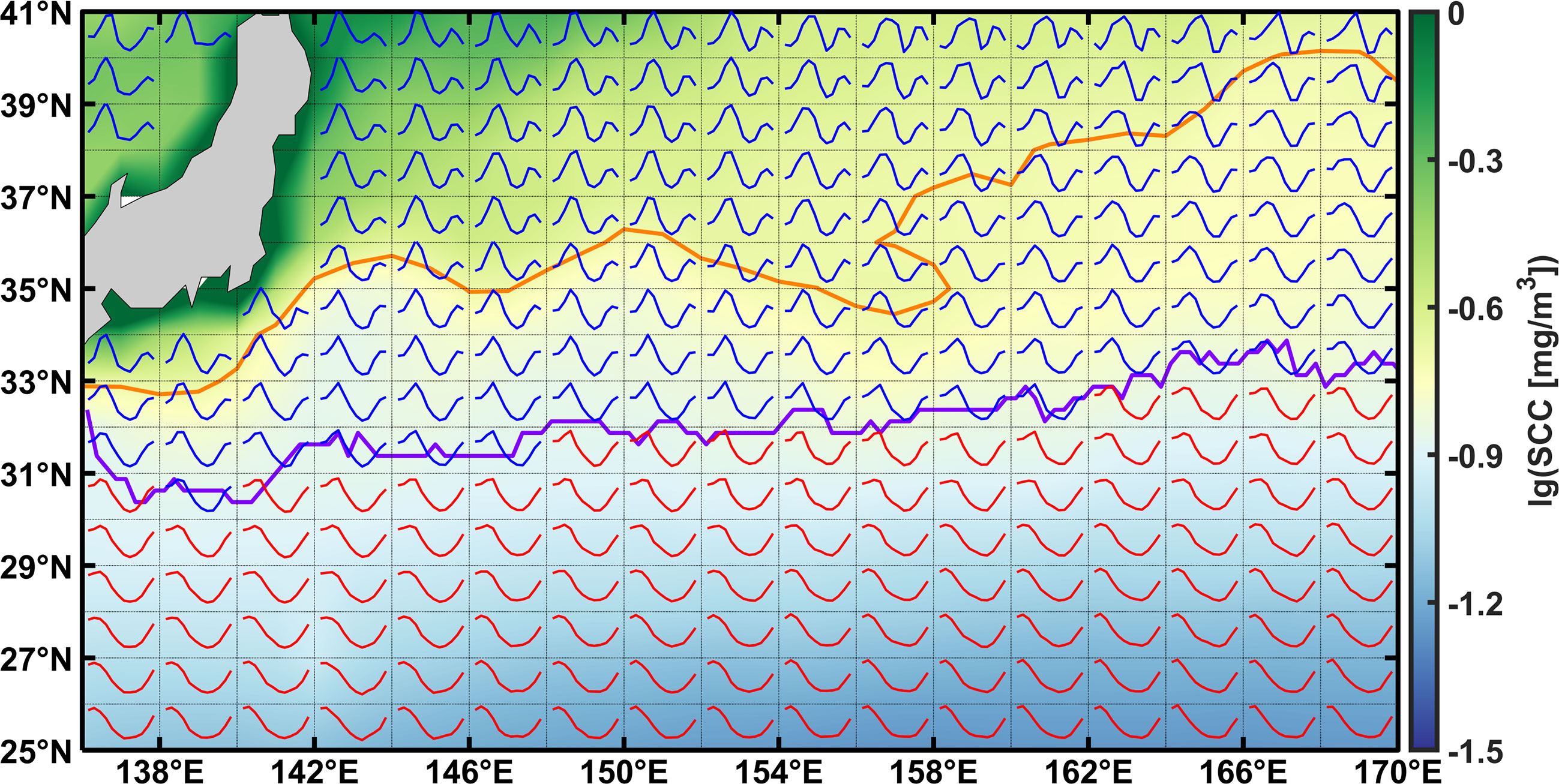
Figure 1 The standardized seasonal cycle of SCC in the KE region. The seasonal cycles of SCC, derived from the monthly averaged data from 2003 to 2018, are plotted within a bin of 2×1°. Colored shadings represent the multi-year-averaged SCC, and the transition zone (i.e., 0.2 mg/m3 contour) is denoted as the bold orange line. The unimodality and bimodality of SCC are indicated by red and blue lines, respectively, and the boundary of them as the bold purple line.
To better understand the quantitative role of the nutrient and light on the regulation of SCC and the future changes of SCC seasonal cycles, we have used 16-year remote sensing data to map the spatial pattern of the SCC seasonal cycle and identify the boundary between bimodal and unimodal variations of SCC in the KE region. The different roles of the nutrient and light in regulating the seasonal variations of SCC have been qualitatively assessed using a mathematically-oriented regression model. The mechanisms accounting for the latitudinal-dependent emergence of SCC seasonal blooms have also been explored. With this model, we provided insights into the switch pattern between bimodality and unimodality of SCC in mid-latitude oceans.
In this study, SCC data were derived from merged multi-sensor satellite remote sensing ocean color observations data in Copernicus Marine Environment Monitoring Service (CMEMS). Level-4 monthly averaged SCC data with 4 km spatial resolution between January 2003 and December 2018 in the KE region (25°N to 41°N, 136°E to 165°E) were used to explore its spatial and temporal variations.
The variations of Nitrate (N) concentration and photosynthetically available radiation (PAR) were used to determine the dominant factors of the SCC seasonal cycle. Due to the limited observation data of seawater N concentration, we employed the PISCES biogeochemical model output of monthly N (mg/m3) in CMEMS Level-4 datasets with 0.25° spatial resolution, and we chose to utilize 0.5m-layer N extracted from 75 levels to be consistent with other variables in depth. Daily and monthly PAR (Einstein/m2·day) data with 4 km resolution were derived from the MODIS-Aqua satellite observations on the National Aeronautics and Space Administration Ocean Color website by Ocean Biology Processing Group (Frouin et al., 1989). Since this study mainly aims to reveal the overall pattern of SCC in the KE region, we used a 1-degree average of SCC data to minimize the mesoscale effect on our result.
In addition, the daily SCC data with a high spatial resolution (0.25×0.25°) derived from the CMEMS model were also used to investigate the lead-lag relationship between SCC and N/PAR. Here, temporal linear interpolation was utilized to fill in the missing values of daily PAR data. The daily optimum interpolation SST (°C) data with 0.25° spatial resolution were obtained from National Oceanic and Atmospheric Administration (NOAA). All daily data spanned from the first day of 2012 to the last day of 2013. Details of data sources are shown in Table 1.
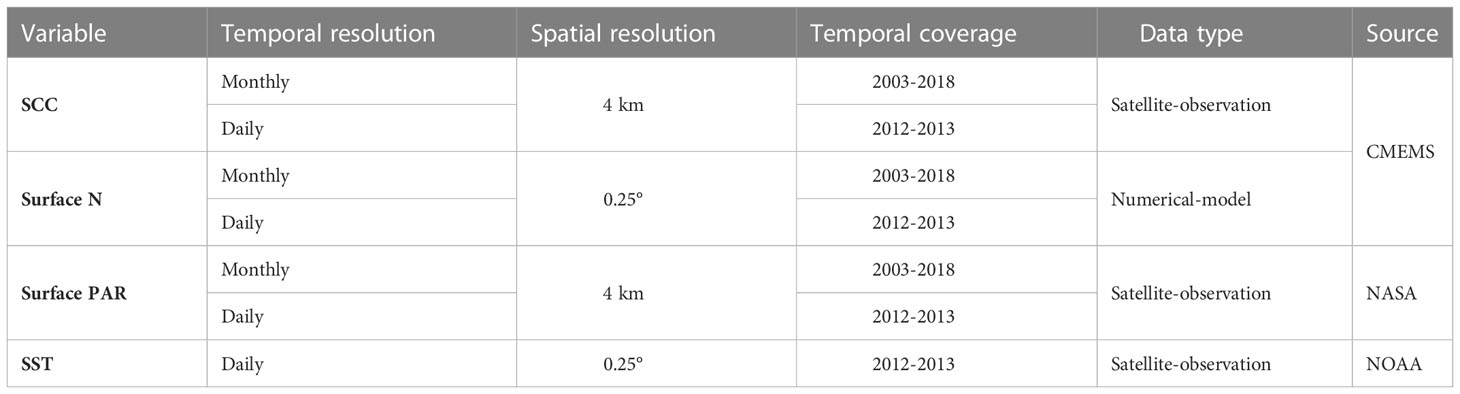
Table 1 Description of data used in the study.
The bimodal/unimodal features of SCC at higher/lower latitudes have been introduced, which are characterized by a coarse zonal boundary at approximately 32°N (Figure 1). To better characterize the month of peaks and valleys at different latitudes, as well as the accurate emerging latitudes of SCC bimodality, we used high-resolution SCC data in the subsequent analysis.
The primary and secondary peak (valley) months are defined as the months when SCC reaches the highest (lowest) value in each season. Generally, the magnitude of spring blooms is larger than fall blooms in the region of SCC bimodality, so the peak occurring from February (August) to July (January) is denoted as primary (secondary) peak. The single peak during a year, usually blooming in early winter in the region of SCC unimodality, is only regarded as the primary peak. The primary (secondary) valley, which usually occurs from May (November) to October (April), can be identified accordingly right after the previous peak.
The spatial pattern of peak/valley months of SCC in the KE region is shown in Figure 2, from which we can easily identify the geographical boundary between the bimodal and unimodal SCC seasonal cycles. It should be noted that, in the KE region, the occurrence of each peak is not synchronous, characterized by up to five (three) months delay as the latitude gets higher (lower) for the primary (secondary) peak. For the primary peak, SCC tends to peak from February to May with the increasing latitudes gradually. Concerning the secondary peak, it displayed an opposite pattern that the occurrence time lags gradually as the latitude gets lower, roughly in late fall and early winter. Unlike the peak, the month of primary (secondary) valley is almost synchronous, occurring in August/September (January). The potential controlling mechanisms of these phenomena will be discussed later.
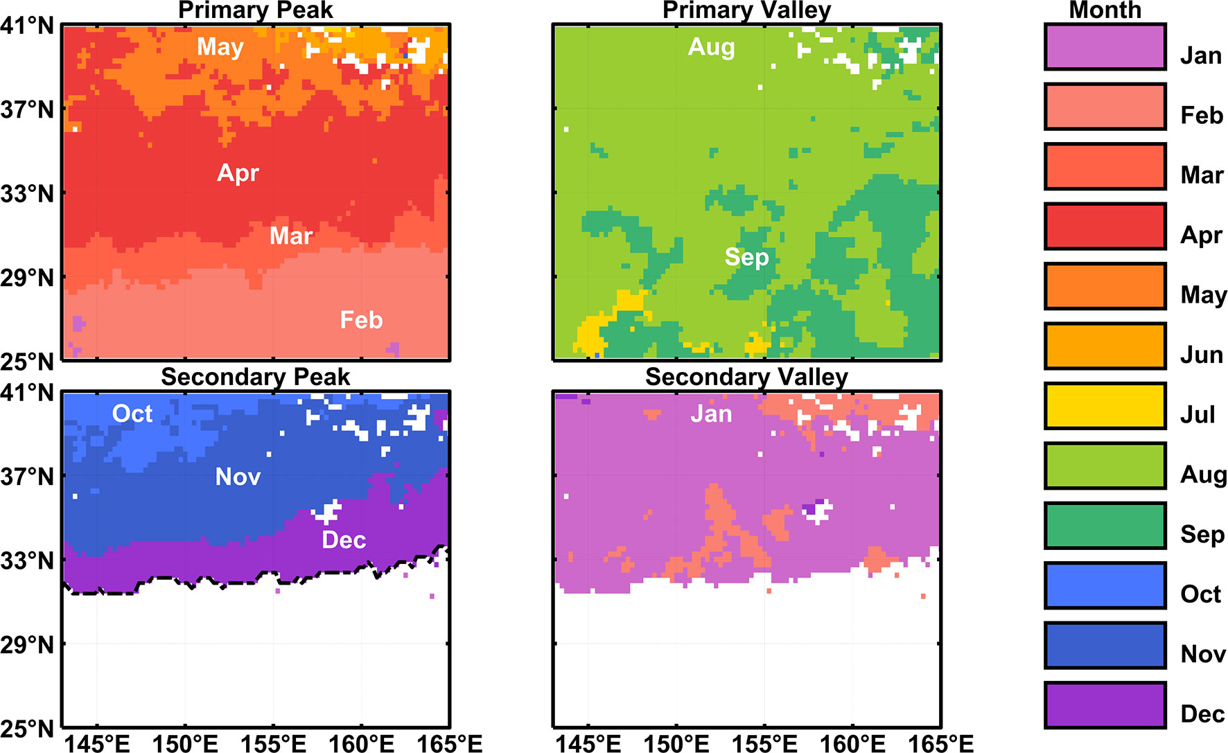
Figure 2 Peak and valley months of SCC seasonal cycle in the KE region.
The above features are similar to the result of Obata et al. (1996), who used Coastal Zone Color Scanner (CZCS) data and defined the bloom time as the month when the pigment concentration doubled compared to the previous month. Differently, in our study, we defined blooms as the peak value point of SCC in each season to avoid swelling caused by occasional processes like typhoons and eddies. Regarding the meridional variation of bloom months, the previous study has noted such a pattern but only analyzed the primary peak, while the zonal difference of SCC peak months was not captured as well (Siswanto et al., 2015). Here we have found that about half of the KE region is characterized by bimodal SCC seasonality. A more accurate characterization of the secondary peak has been formed based on the latest satellite observations available and the northward shifting feature of secondary peak months has been revealed as the longitude increases.
To better understand the above-mentioned features and explicitly identify the role of decisive factors, we proposed a simple regression model to reconstruct the seasonal cycle of SCC. Here, only two key factors, N and PAR, were selected as the input, and their seasonal cycles are shown in Figures 3A, B. It is worth noting that the impact of temperature was ignored in this model, not only because it is shown to be less important in regulating the spatial-temporal variations of SCC compared with nutrients and light based on the basin-scale model results (Wang et al., 2009), but also the temperature-growth relationship could be overestimated by laboratory experiments, as the dominate phytoplankton community in natural conditions could adapt better to the ambient temperature at large scales (Sherman et al., 2016). Also, there is a strong co-variation between temperature and PAR/N through heating and stratification. This co-variation makes the effects of temperature inseparable, going against the fundamental principle of independence in linear regression. The effects of PAR were categorized as direct and indirect ones, which represent biological and physical effects, respectively. In this model, we focused on the direct effect of PAR that is independent of N.
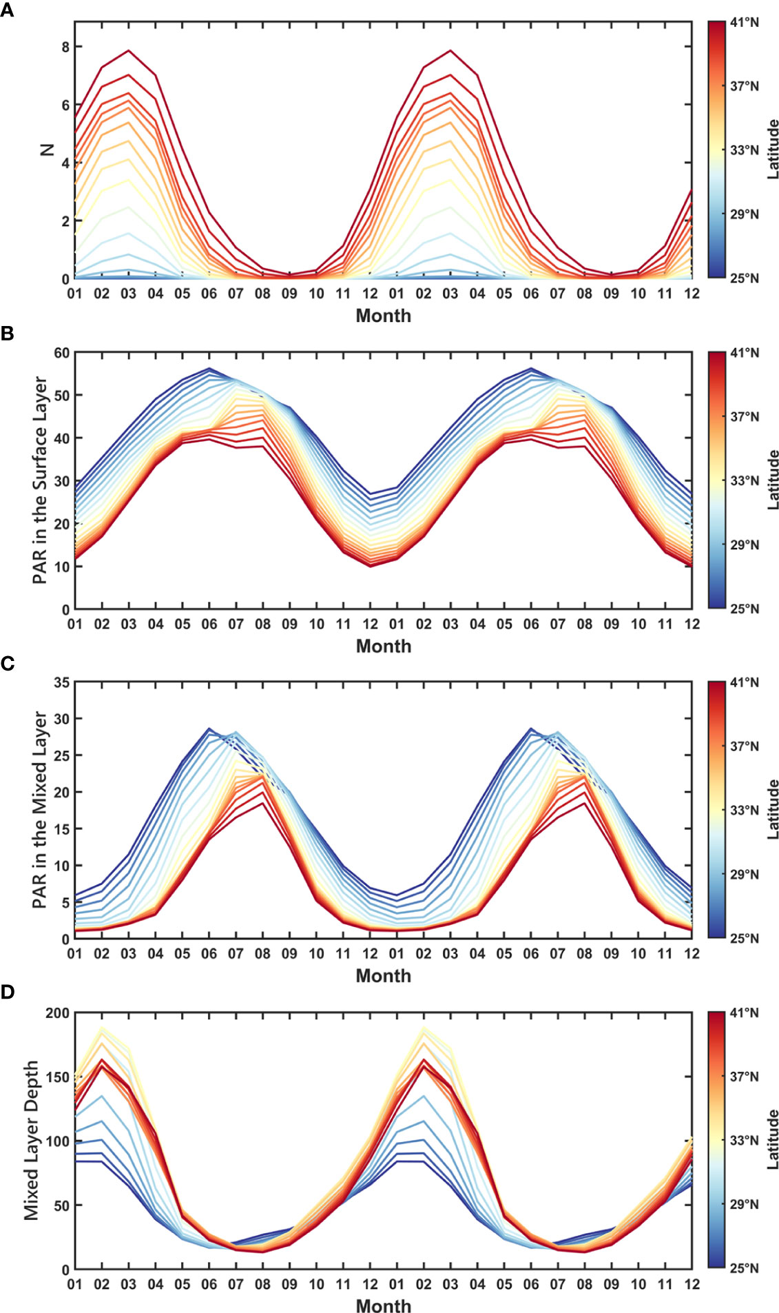
Figure 3 Seasonal cycle of (A) N, (B) PAR in the surface layer, (C) PAR in the mixed layer, and (D) Mixed Layer Depth.
A series of previous laboratory studies have formulated the nutrient- and light-dependent functions of growth rate or phytoplankton biomass to separate the effects of each single factor. Classical models consider growth rate as an asymptotic function of N. Specifically, the growth rate increases with N before gradually reaching a saturation value (Monod, 1942; Droop, 1973; Morel, 1987). Phytoplankton biomass as a function of N can be calculated by the definition of growth rate as a Logistic growth equation in Eq. (1) (Tsoularis and Wallace, 2002):
where µ is the growth rate, B and K are biomass and the maximal population size at carrying capacity, and t is the time. Considering the time duration dt stays unchanged and that the growth rate matches well with the Michaelis-Menten equation (Figure 4A), the integration in time is shown in Figure 4B. It is worth mentioning that N is a limiting nutrient in most open oceans (Sambrotto et al., 1993), hence the phytoplankton biomass exhibits an exponential relationship with N. With regard to PAR-related biomass, a classical function can be constructed based on the relationship that phytoplankton biomass increases and then decreases along with the intensification of light (Ryther and Menzel, 1959; Steele, 1962; Platt and Gallegos, 1980), as shown in Figure 4C.
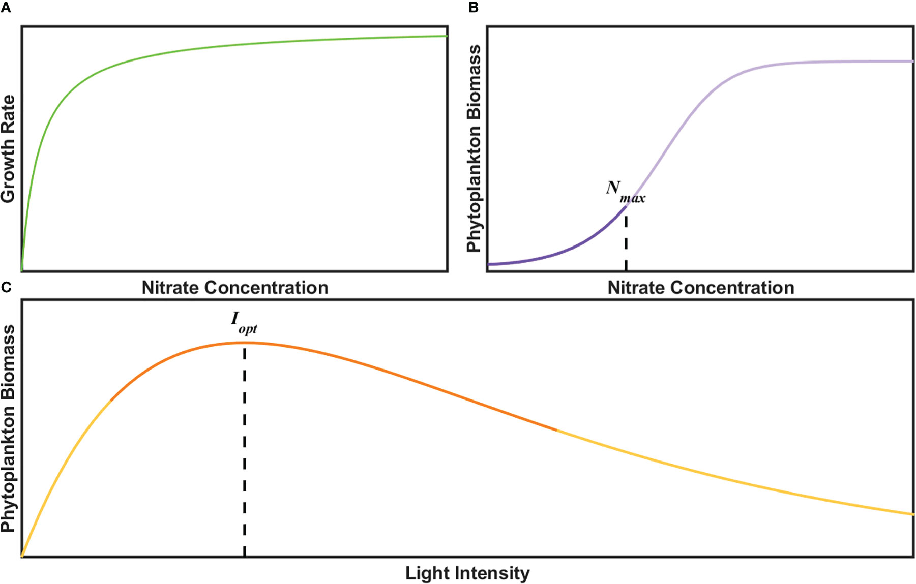
Figure 4 Schematic graph of (A) growth rate, (B) phytoplankton biomass as a function of N concentration according to Michaelis-Menten equation and (C) phytoplankton biomass as a function of light intensity with Steele equation. The bold lines represent multi-year averaged range of N and PAR in x-axis.
As is shown in Figures 4B, C, it is a reasonable and simple way to describe the relationship between phytoplankton biomass (indicated by SCC) and N/PAR with quadratic equations in the form of y = a(x–b)2 + c. Before we established the model, all variables were averaged into a box of 1×1°, and then a base-10 logarithm was applied to SCC and N. Each variable was finally normalized in a range of 0 and 1 (noted as N', PAR' and SCC'). It should be noted that N'=0/PAR'=0 (N'=1/PAR'=1) is the lower (upper) bound of N/PAR. Here we proposed two dependent functions, f(N) and g(PAR), which represent the response of SCC to N and PAR, respectively. To better reveal the relative importance of each factor, these two functions are represented as follows ranging from 0 to 1 (Figure 5):
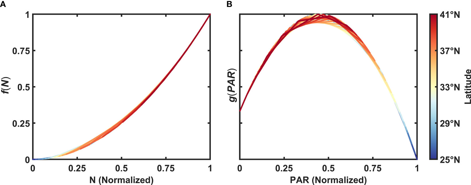
Figure 5 Normalized SCC responses to (A) N and (B) PAR.
The selection of specific coefficients in Eq. (2) was based on the statistical relationship between SCC' and N' by fitting all these data we used in our model with the quadratic equation y = a(x–b)2 + c, and that of Eq. (3) was based on the statistical relationship between SCC' and PAR'–1 data with the same equation. In the function of g(PAR), it is more effective to reproduce the seasonal cycle of SCC' as we use the PAR' one month in advance (i.e., PAR'–1, Lag=1), which will be discussed later.
To further identify the role of N and PAR at different latitudes and their relationship with the diverse seasonal cycles quantitatively, a regression model was adopted to reconstruct the SCC annual cycle at different latitudes, based on the two functions above:
where k1, k2, and b are constants only dependent on latitudes, obtained from curve fitting at designated latitudes ranging from 25°N to 41°N. k1 and k2 represent the relative contribution of the nutrient and light to SCC', respectively. b is to adjust the SCC' seasonal cycle within an acceptable range between 0 and 1. Comparing the normalized seasonal cycle of observed SCC' shown in Figure 6A, the regression model well reproduces the general features of seasonal cycles at different latitudes in both magnitude and phase with a high coefficient of determination R2 = 0.96 (Figure 6B). In particular, the model reasonably captures the peak and valley months, and the shift pattern of peaks as the latitude gets higher, as well as the transition latitudes from unimodal to bimodal seasonal cycles. If we use the concurrent monthly PAR' (Lag=0) as the input, as shown in Figure 6C, the regression model fails to capture the characteristic of the bimodal pattern at higher latitudes. More discussions on this issue will be addressed in section 4.1.
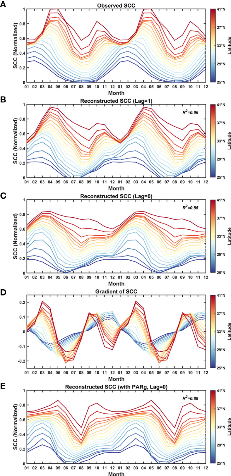
Figure 6 Seasonal cycle of (A) Observed SCC, (B) Reconstructed SCC using PAR and N with PAR one month ahead of SCC, (C) Reconstructed SCC with concurrent PAR, (D) Gradient of observed SCC and (E) Reconstructed SCC with concurrent PARg, at different latitudes. The seasonal cycles of SCC are generated by averaging the data from 2003 to 2018 between 143°E-165°E.
To investigate the relative role of N and PAR at different latitudes, the relative values of coefficients k1 and k2 are shown in Figure 7, representing the weight of N and PAR in contributing to the seasonal cycles of SCC. As for N, it can be well identified that the relative contribution of the nutrient, i.e., k1/(k1+k2), to the seasonal cycle of SCC moderates from subtropical to mid-latitudes, and stabilizes relatively north of 35°N. Whereas PAR follows an opposite pattern. It should be emphasized that the crossing latitude of these two curves, as shown in Figure 7, resides at approximately 31.6°N, where the relative contributions of the nutrient and light are equally important. The crossing latitude is close to the mean boundary between unimodality and bimodality roughly at 32.1°N in Figure 2.
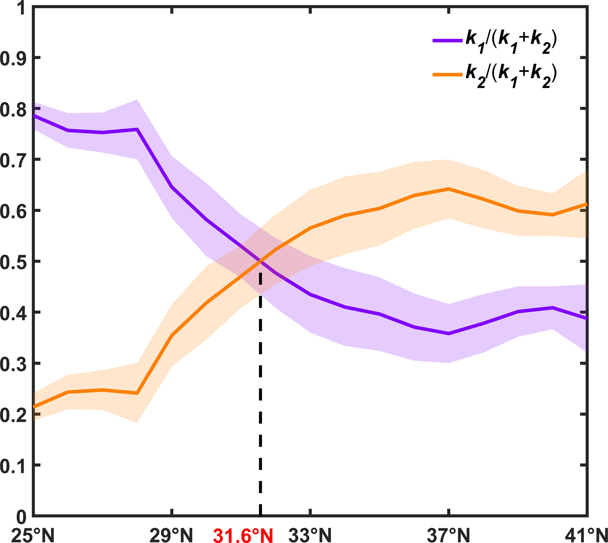
Figure 7 Relative values of coefficients as a function of latitudes. The bold lines indicate the relative values of coefficients derived from multi-year averaged seasonal cycles at different latitudes. The shading areas denote the standard deviations of coefficients calculated from the seasonal cycle of each year at different latitudes.
To further explain the emergence latitudes of bimodality and their northward shifting pattern as the longitude gets higher, the regression model was then applied to the seasonal cycles of SCC at different longitudes. It is shown in Figure 8 that the general features of relative contributions from N and PAR are similar at different longitudes. However, the crossing latitude moves northward in a wavy manner, which indicates the gradual dominance of N in forming the seasonal cycle of SCC.
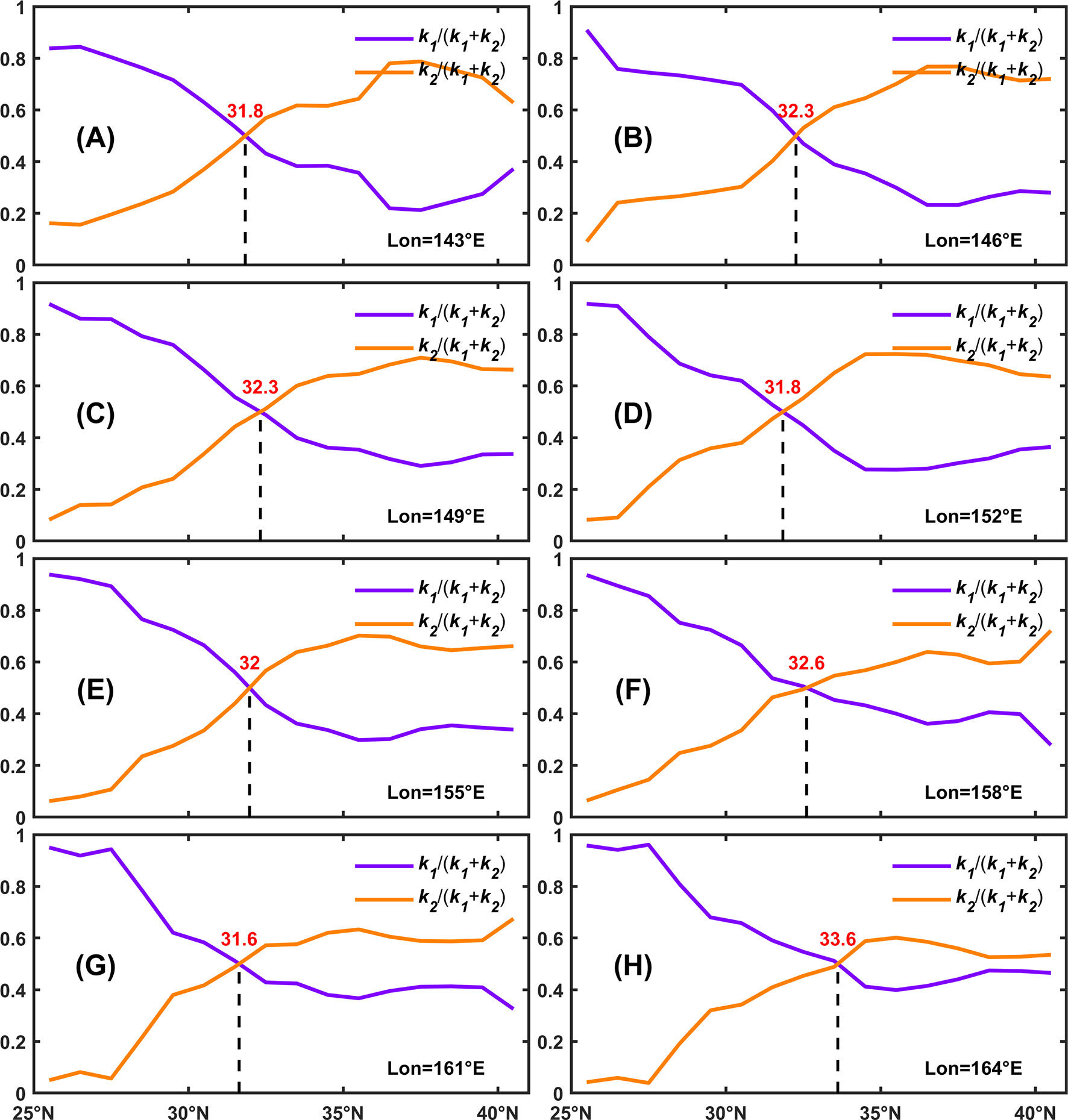
Figure 8 Relative values of coefficients as a function of latitudes at (A) 143°E, (B) 146°E, (C) 149°E, (D) 152°E, (E) 155°E, (F) 158°E, (G) 161°E and (H) 164°E. The bold lines indicate the relative values of coefficients derived from multi-year averaged seasonal cycles at different latitudes. The shading areas denote the standard deviations of coefficients calculated from the seasonal cycle of each year at different latitudes.
The rough coincidence of the crossing latitude from the model and the emergence latitude of the fall bloom from observations implicates the hidden role of N and PAR in setting up bimodality of the SCC seasonal cycle. To confirm this relation, we further calculated the two boundaries and found a close relationship between them with a correlation over 0.7 (Figure 9). Therefore, the emergence of the fall bloom (i.e., secondary peak) can be explained as a critical state where N and PAR contribute equally to the seasonal cycle of SCC in this model.
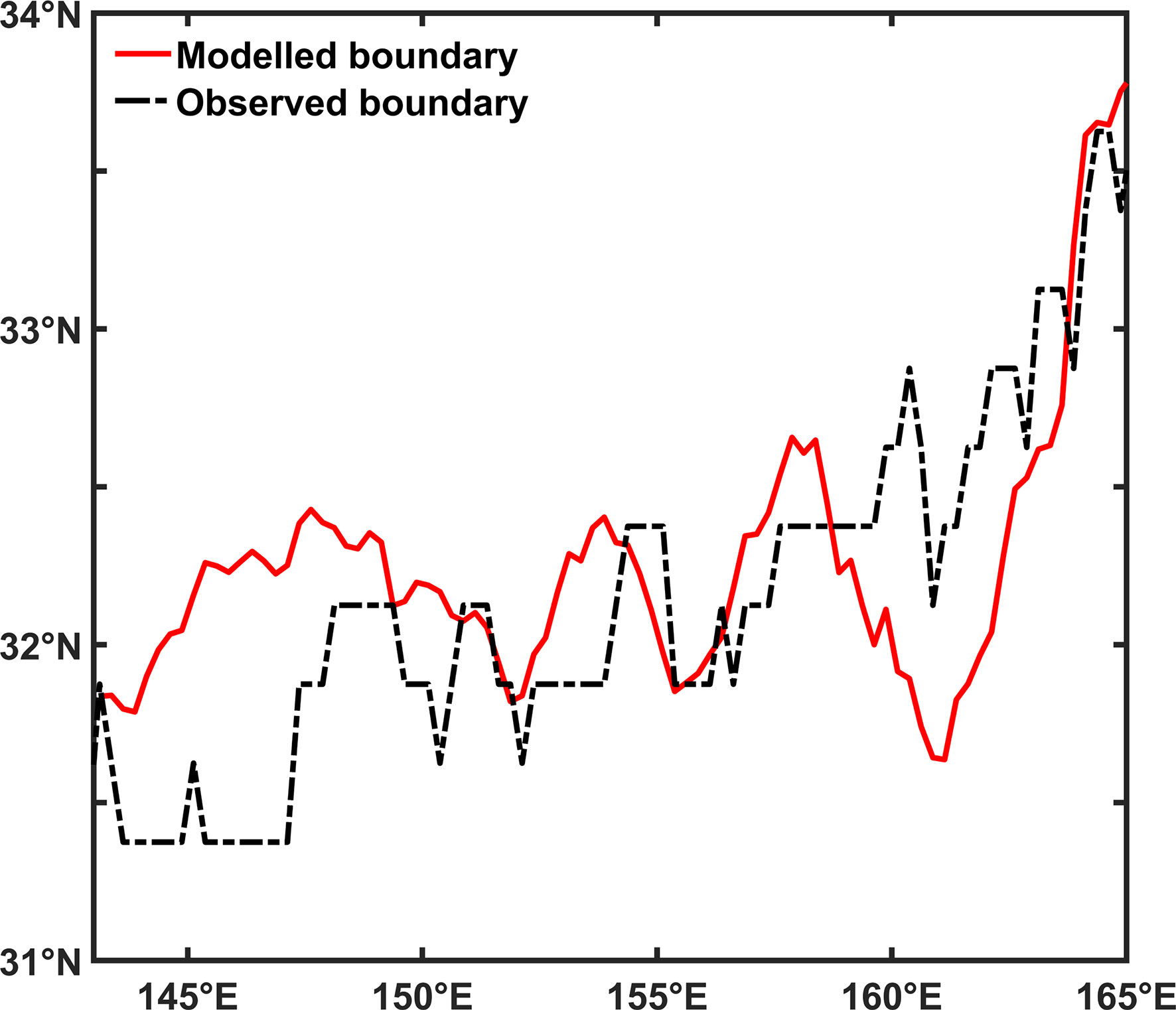
Figure 9 The modelled crossing latitude and the observed boundary between bimodality and unimodality at different longitudes.
The seasonal cycle of SCC has been simulated by a variety of models, either simple or complex, to study the controlling factors of SCC variations. However, most of these models have involved multiple factors but still have not well reproduced the magnitude and the phase of fall blooms. Without considering the one-month lag effect of PAR, we also met a similar problem as reported in previous studies (Kim et al., 2007; Xiu and Chai, 2012), i.e., the seasonal cycle of SCC is not properly simulated especially at higher latitudes (recall Figure 6C), which illustrates that the phase difference between PAR and SCC (termed as the lag effect of PAR on SCC) might be decisive in simulating seasonal cycles across varying latitudes. The phase difference has also been found to be several days long in the nearshore regions (Trombetta et al., 2019; Moradi, 2020), but little is known about the month-scale lag effect in open oceans.
To understand the reason for the inadequate representation of the SCC seasonal cycle by using the regression model in Figure 6C, we adopted a lead-lag correlation regarding the PAR and SCC to explore the lead-lag effects of physical and non-physical processes. Considering that the nonlinear lag effects might exist in the transition regions from unimodal to bimodal seasonal cycles, the northernmost (41°N) and southernmost (25°N) latitudes were selected, which are characterized with the most obvious lag and non-lag effects. The correlation between PAR and SCC involves many processes, among which physical processes can be understood as follows: PAR regulates SST via thermal heating, then SST regulates surface N through vertical stratification, and finally N regulates SCC. Suppose there are only physical processes, the integral of the lag time in the above three physical processes should be consistent with the lag time of total processes between PAR and SCC.
The actual consequences are as follows: At 25°N, the SCC varies concurrently with PAR, i.e. the lead-lag correlation is highest when the lag is 0 day (Figure 10A). Considering the physical processes mentioned above are synchronous as well (Figures 10C, E, G), PAR exhibits no lag effect on SCC at lower latitudes. At 41°N, as shown in Figure 10B, PAR is about 105 days ahead of SCC. In terms of physical processes, however, PAR leads SCC only by 76 days, which is regarded as a linear superposition of the following lag time among the factors: (1) PAR leads SST by 58 days due to the required time of energy transfer from sunlight to seawater, (2) SST leads N by 13 days due to the mixing time for N entrainment, and (3) N leads SCC by 5 days due to phytoplankton growth (Figures 10D, F, H). These timescales are consistent with those of the general heating process lasting for about two months (Prescott and Collins, 1951) and the phytoplankton response to nutrient supply of about a week (Shi et al., 2012; Zhang et al., 2019). The resultant 29-day difference between total and physical processes implies that non-physical lag does exist, and we consider it as a biological process. Earlier in section 3.2, we mentioned that we focused on the biological effect of PAR which is independent of N, and only acts on SCC in our regression model. We further calculated the gradient of SCC (Figure 6D) which partly represents the growth rate, and found the gradient was one month ahead of SCC at higher latitudes. The response time of the growth rate to PAR is generally at a second or hour scale (Reynolds, 1990), and can be considered as a simultaneous process in our study. Therefore, this one-month biological lag between the growth rate and SCC likely accounts for the phenomenon that the bimodal SCC seasonal cycle is reproduced at higher latitudes only with PAR leading by one month.
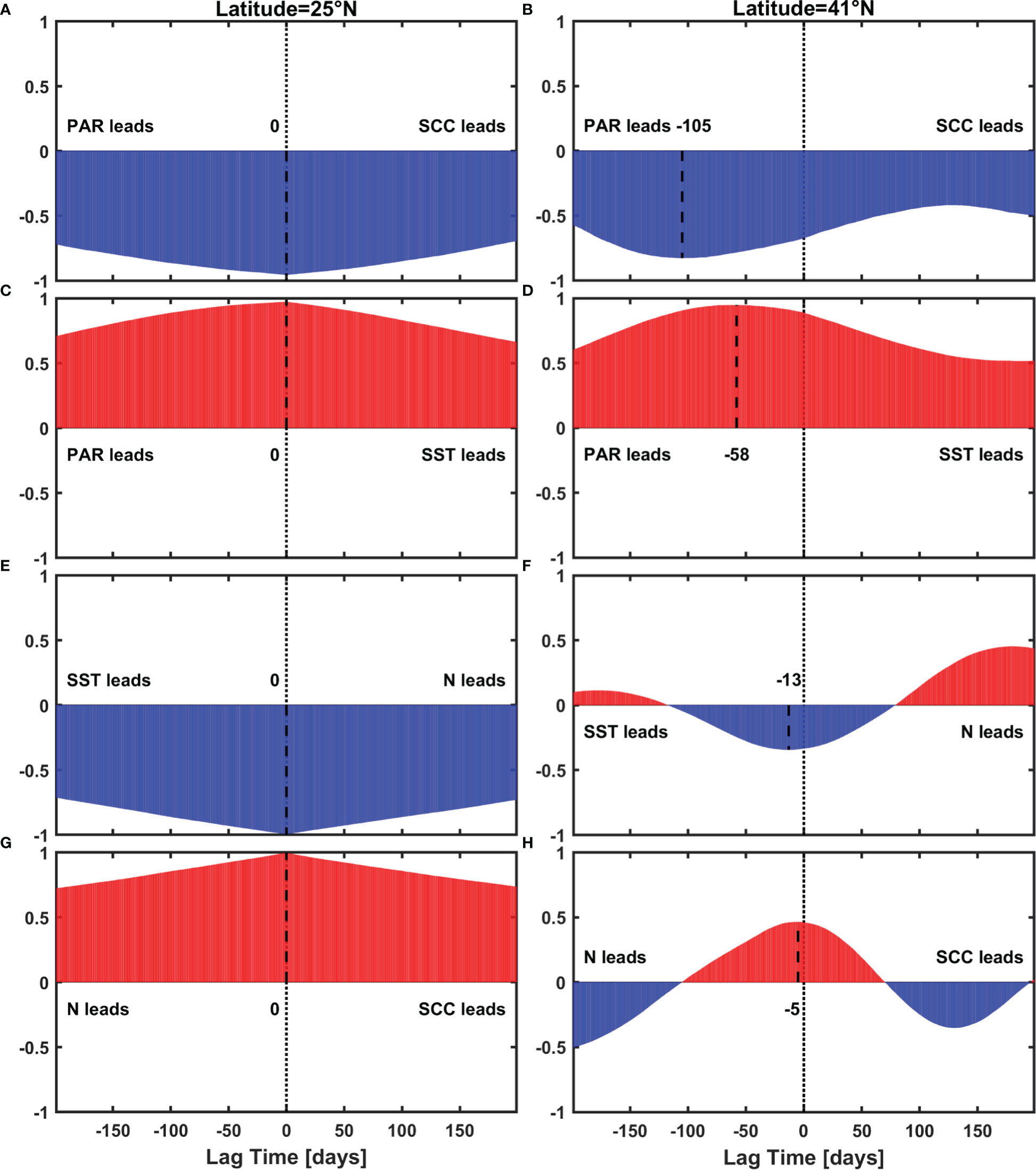
Figure 10 Lead-lag correlation result between (A), (B) PAR and SCC (C), (D) PAR and SST, (E), (F) SST and N, (G), (H) N and SCC, at 25°N (left module) and at 41°N (right module), black dash lines indicate the maximum correlation.
Mixed Layer Depth (MLD) is usually considered as a dynamic process that impacts SCC by modulating the vertical distribution of phytoplankton (Figure 3D). This mixture has the potential to redistribute the Chl profile, resulting in subsurface Chl-driven changes in SCC (Letelier et al., 2004; Xing et al., 2021). In this condition, Chl and N are quasi-homogeneous in the MLD (Kara et al., 2003; de Boyer Montégut et al., 2004). On the contrary, PAR has a rapid attenuation in the mixed layer. Therefore, we applied the USRGR model of Xing et al. (2022) to combine with the monthly diffuse attenuation coefficient at 490nm (Kd490) from MODIS-Aqua sensor and MLD data from BOA-Argo, to calculate the averaged PAR in the MLD (PARg, Figure 3C), aiming at illustrating the effect of PAR in the mixed layer in our model.
The result is shown in Figure 6E, a bimodal seasonal cycle of SCC at higher latitudes can be reconstructed without a lag time, and thus it could be another explanation for the lag effect of PAR. In addition, we also analyzed the lead-lag correlation between PARg and SCC with PARg calculated with daily numerical-model MLD data from CMEMS, and found lag time between PARg and SCC in the total process was almost synchronous with that in physical processes at both lower and higher latitudes (Figure 11).
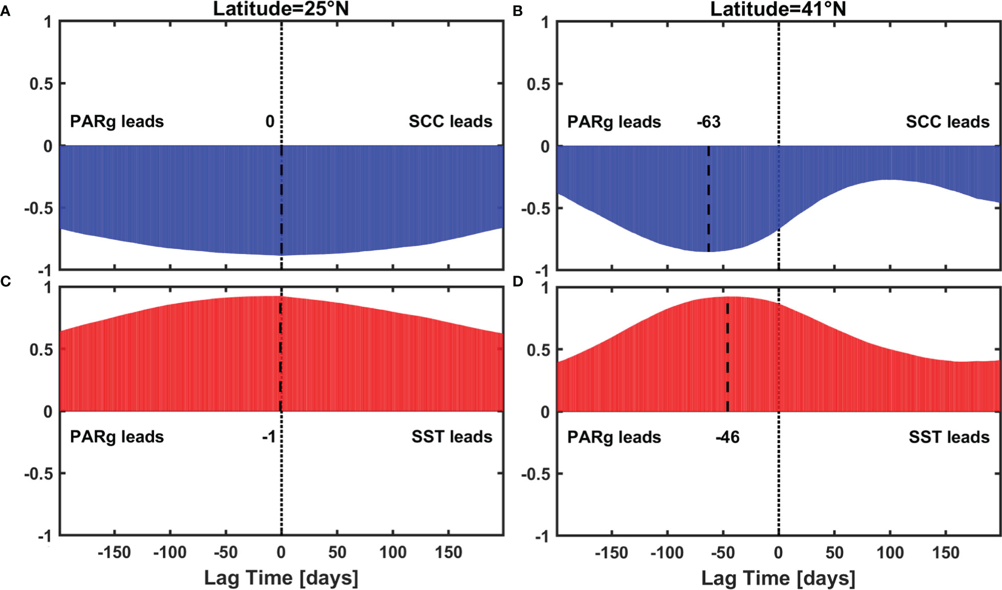
Figure 11 Lead-lag correlation result between (A), (B) PARg and SCC (C), (D) PARg and SST, black dash lines indicate the maximum correlation.
However, the model using PARg performs not as well as the original model in winter and spring, partly because PARg is a function of MLD, which makes PARg unable to be independent of N, inconsistent with the fundamental principle of linear regression. In winter and spring, PAR is decisive to SCC and MLD varies sharply, leading to PARg being more related to N through MLD. Additionally, although the SCC data we used in our study were derived from merged multi-sensor satellite and monthly averaged, we cannot uncover whether these snapshots can represent Chl in the MLD, hence further studies are necessary to explore the relationship between satellite-derived Chl and average Chl in the mixed layer.
Our study has found that N is the primary factor that affects the emergence latitude of the fall bloom while PAR is suitable. At the same latitude, PAR generally changes little at different longitudes, while N decreases constantly moving forwards to the open ocean (Figures 12A, B). According to the result of our model shown in Figure 8, as it moves eastward, the relative role of N becomes stronger, consequently that of PAR becomes weaker, leading to the northward heading of the intersection of two lines. Another evidence is the overlap between the emergence latitude and the contour of N concentration of 10-1.2 mmol/m3 averaged during the fall season (from October to December) in Figures 12A, B. Here we compared the boundaries identified by averaged seasonal cycles of the first five years (2003 to 2007) and the last five years (2014 to 2018), and found that the tendency of boundary coincides with that of 10-1.2 mmol/m3 N isoline, moving northward from 31.5°N to 32.4°N and 31.3°N to 32.2°N, respectively. The coincidence of position and tendency between boundary and N suggests that the fall blooms are mainly triggered by the transportation of nutrients from the deep layer to the upper ocean when light is still suitable, consistent with the conclusion of the previous study (Obata et al., 1996). This is different from spring blooms triggered by light intensification when nutrients are still available. In the east of the KE region, the circumstance is similar to that in the lower latitude region: N dominates the seasonal cycle of SCC when it is in short supply, therefore the phenomenon of bimodality in the west and unimodality in the east exists at the same latitude around the boundary, determining the southwest-northeast direction of fall bloom latitudinal boundary.
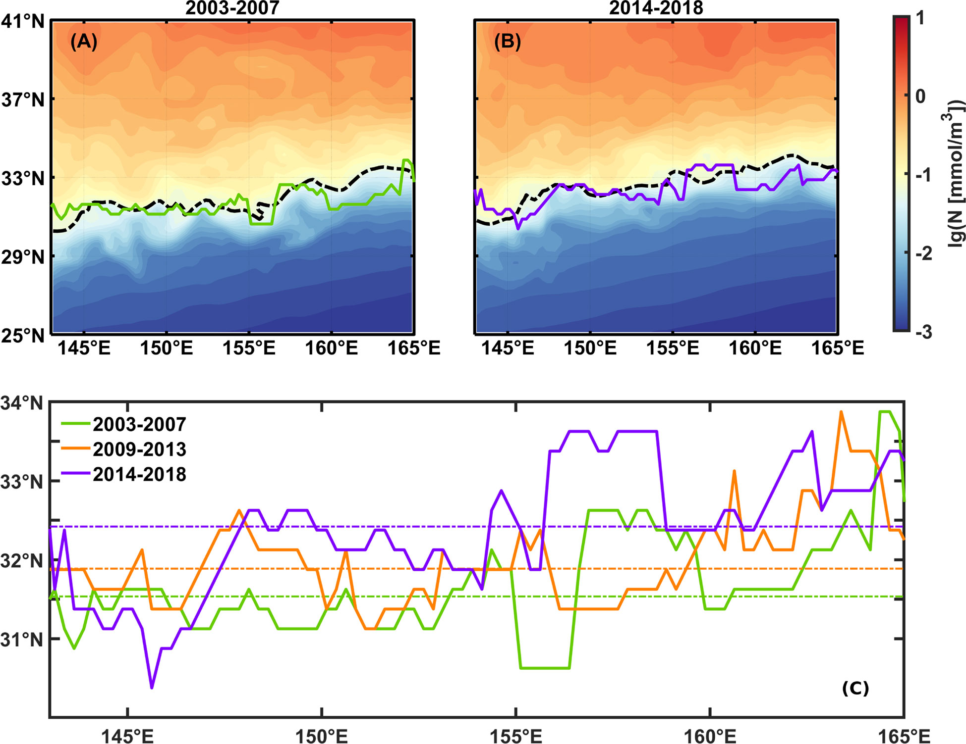
Figure 12 Emergence boundaries of fall blooms and averaged surface 10-1.2 mmol/m3 N (broken black line) in fall (October-December) averaged during (A) 2003 to 2007, (B) 2014 to 2018, the emergence latitudes of the fall bloom (solid line), and averaged surface N in fall (shading), and (C) the comparison between three boundaries, broken lines indicate average latitude of each boundary.
Combing the light-controlled spring bloom result with our nutrient-dominant fall bloom result, we can explain the phenomenon in Figure 2 that primary (secondary) bloom starts later (earlier) as the latitude gets higher. As shown in Figure 13, we used Hovmöller diagrams to describe the changes of representative PAR or N isoline with latitude and month. In spring, the isoline PAR=39 Einstein/m2·day delays as latitude increases, leading to bloom time varying from February to May in succession. On the contrary, in fall, the N=10-1.2 mmol/m3 isoline advances as latitude increases, leading to bloom time varying from December forward to October.
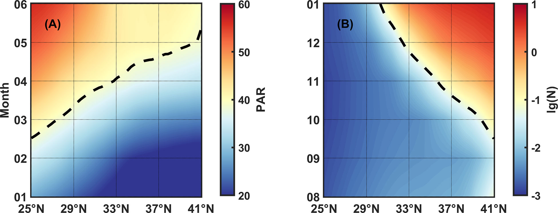
Figure 13 (A) PAR and (B) N varying with latitudes and months. Color represents the values of PAR and N, the broken lines indicate isoline PAR=39 Einstein/m2·day and N=10-1.2 mmol/m3, respectively.
Under the context of global warming, we have reckoned the tendency of SCC in the KE region on the basis of the conclusions drawn above. It is generally supposed that global warming has an uncertain effect on PAR that consists of both a boost from positive feedback (Loisel et al., 2012) and an offset from opaque types of clouds (Bala et al., 2011), while N in the upper ocean is almost certainly lower due to the enhanced stratification (Behrenfeld et al., 2006; Polovina et al., 2008; Thomas et al., 2017). Excluding the fluctuations of PAR, we only concentrated on the probable consequences of decreased N in the upper layer in the global warming scenario.
The first effect is the magnitude of SCC. The magnitude of SCC would become lower in lack of N for the whole year. In the previous study, it has been found that increasing SST would weaken the mixing process, leading to an obvious decrease of N and SCC in the surface layer (Watanabe et al., 2005). In section 4.1, we found that physical responses are swifter at lower latitudes than at higher latitudes, therefore, the decrease of SCC is exacerbated due to the rapid response of a thin mixed layer here. As for the fall bloom, its magnitude might not be decided by the spring bloom because the consumption in summer is also crucial (Mikaelyan et al., 2017). Secondly, the emergence boundary of fall blooms would move northward according to our results, considering that the general decrease of nutrients has the potential to broaden nutrient-limited regions, which has been substantiated by previous studies that the area of least productivity has expanded by 0.9% per year from 1998 to 2018 (Meng et al., 2021), and up to 2.2% per year from 1998 to 2006 in the oligotrophic gyre of North Pacific (Polovina et al., 2008). In our study, we also found a northward movement of the boundary at a rate of 8.3 km per year approximately in Figure 12C, with averaged SST increasing from 20.9°C, 21.0°C to 21.2°C. The increasing SST intensified stratification, depressed surface N, and led to a northward movement of N isoline. Due to the dominant role of N isoline in the emergence boundary of fall blooms, the boundary moves northward correspondingly.
The change in the magnitude and the coverage of fall blooms have the potential to influence air-sea carbon exchanges, according to the seasonal distribution of averaged surface water-atmospheric partial pressure difference (ΔpCO2) from 2003 to 2016. In general, the seasonal cycle of ΔpCO2 in the KE region is closely associated with SST, MLD, and biological activities (Ishii et al., 2014). As shown in Figure 14, phases and seasonal features of ΔpCO2 are similar to those of SCC with bimodality and unimodality at higher and lower latitudes. This implies the key role of the biological effect in regulating ΔpCO2 in this region. Moreover, the carbon sink might be less efficient due to not only the decrease of dissolved inorganic carbon, but also the northward movement of the boundary and the consequent contraction of fall carbon sinks under the context of global warming. Meanwhile, substantial and high-resolution ΔpCO2 data is further needed to investigate the change of emergence latitude.
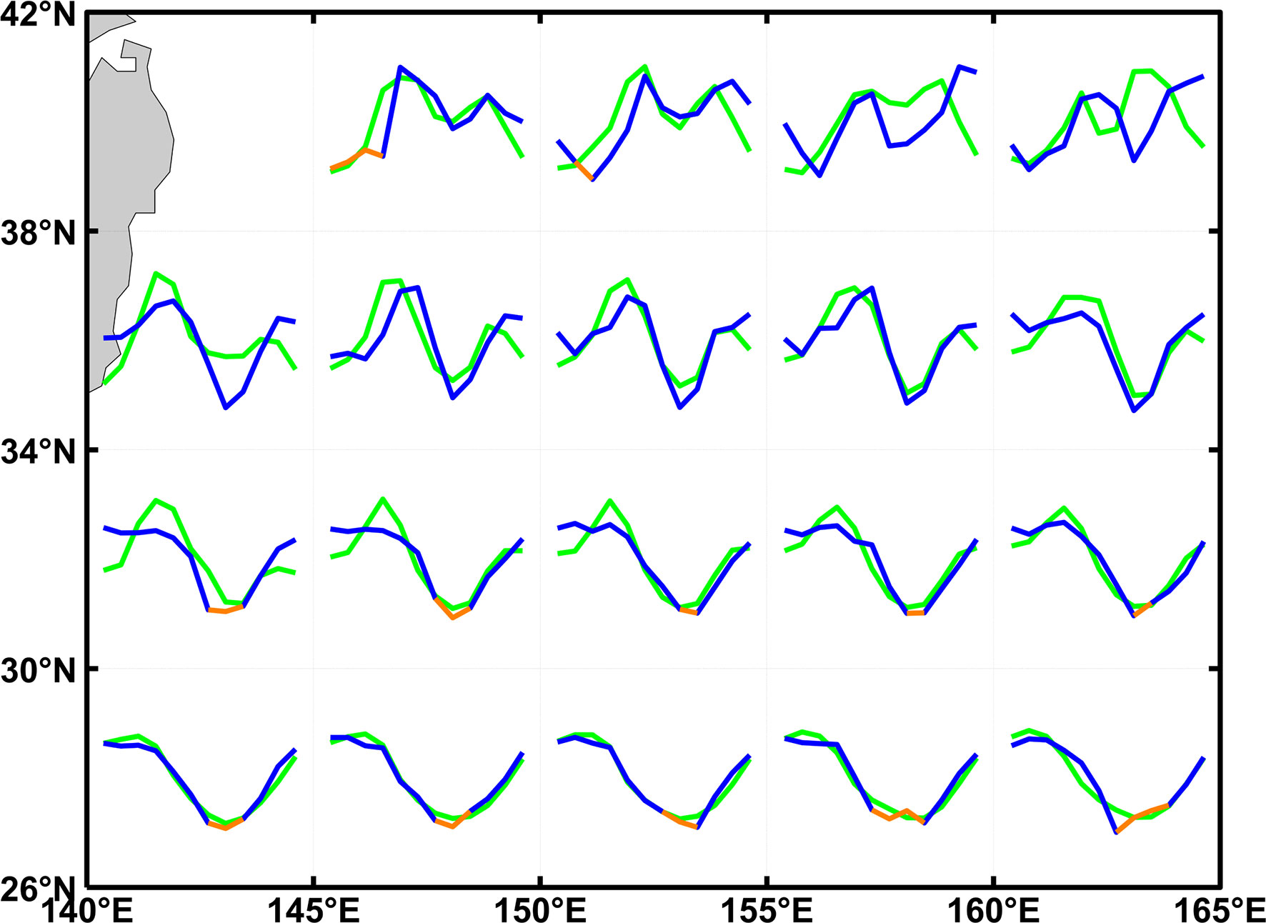
Figure 14 The averaged seasonal cycle of standardized surface oceanic-atmospheric partial pressure difference (blue and orange) and SCC (green) from 2003 to 2016, orange (blue) color means ΔpCO2<0 (ΔpCO2>0) and ocean serves as a carbon source (sink).
In this study, we have investigated the seasonal cycle of SCC at different latitudes in the KE region and explored the impacts of two fundamental factors, N and PAR, on the unimodal-to-bimodal switching latitudes with both the remote sensing data and numerical data. We have found that bimodal and unimodal peak seasonal cycles exist at higher and lower latitudes respectively. It is found that the month of primary bloom delays northward from February to May but that of secondary bloom delays southward from October to December, which can be explained by the isoline of PAR and N respectively. SCC generally reaches the minimum in August in the whole region and the second minimum in January in the region with double peaks. To demonstrate the effect of the nutrient and light on SCC, we reconstructed SCC with a mathematical model, which can generally reveal the features of seasonal cycles at different latitudes. The coefficient analysis of N and PAR in the model shows that N dominates the seasonal cycle of SCC at lower latitudes while PAR dominates that at higher latitudes. The comparable contribution of N and PAR to SCC variations, which is represented as the boundary between bimodality and unimodality, shows a northward moving characteristic with increasing longitude (31.5°N-33.5°N approximately). We categorized the impacts of PAR on SCC as physical and biological processes, and the contribution of each process differed regionally. Especially, there is about a 30-day lag time induced by biological processes at higher latitudes but no obvious lag time at lower latitudes. Apart from the light-induced change in the extent of ocean stratification, light attenuation within the mixed layer and the interval between growth rate and SCC peak contribute to modulating the lag phase of reconstructed SCC. The well-constructed model that elucidates the pattern of the SCC seasonal cycle can help us better evaluate the changes of air-sea carbon exchanges and associated carbon export in the KE region, characterized by an important carbon sink, especially in the context of intensified global warming.
The original contributions presented in the study are included in the article/Supplementary Material. Further inquiries can be directed to the corresponding author.
ZC contributed to the design of the study. XS performed the statistical analysis and wrote the first draft of the manuscript. All authors contributed to the article and approved the submitted version.
This research is financially supported by the National Natural Science Foundation of China (42225601, 42076009), and Fundamental Research Funds for the Central Universities (202072001). ZC is partly supported by the Taishan Scholar Funds (tsqn201812022).
We thank Bingrong Sun and Yongzheng Liu for their guidance and suggestion from their perspectives of the field of study, thank Zhiyuan Gao and Qirong An for helping data collection in this study, and thank Tiantian Zheng for helping to polish the language. Also, we thank the reviewers for improving this manuscript.
The authors declare that the research was conducted in the absence of any commercial or financial relationships that could be construed as a potential conflict of interest.
All claims expressed in this article are solely those of the authors and do not necessarily represent those of their affiliated organizations, or those of the publisher, the editors and the reviewers. Any product that may be evaluated in this article, or claim that may be made by its manufacturer, is not guaranteed or endorsed by the publisher.
The Supplementary Material for this article can be found online at: https://www.frontiersin.org/articles/10.3389/fmars.2023.1027710/full#supplementary-material
Antoine D., André J., Morel A. (1996). Oceanic primary production: 2. estimation at global scale from satellite (Coastal zone color scanner) chlorophyll. Global Biogeochem. Cycles 10 (1), 57–69. doi: 10.1029/95GB02832
Bala G., Caldeira K., Nemani R., Cao L., Ban-Weiss G., Shin H. (2011). Albedo enhancement of marine clouds to counteract global warming: Impacts on the hydrological cycle. Climate Dynamics 37 (5-6), 915–931. doi: 10.1007/s00382-010-0868-1
Behrenfeld M. J., O Malley R. T., Siegel D. A., McClain C. R., Sarmiento J. L., Feldman G. C., et al. (2006). Climate-driven trends in contemporary ocean productivity. Nature 444 (7120), 752–755. doi: 10.1038/nature05317
Bindloss M. E. (1976). The light-climate of loch leven, a shallow Scottish lake, in relation to primary production by phytoplankton. Freshw. Biol. 6 (6), 501–518. doi: 10.1111/j.1365-2427.1976.tb01642.x
Coma R., Ribes M., Serrano E., Jiménez E., Salat J., Pascual J. (2009). Global warming-enhanced stratification and mass mortality events in the Mediterranean. Proc. Natl. Acad. Sci. U.S.A. 106 (15), 6176–6181. doi: 10.1073/pnas.0805801106
de Boyer Montégut C., Madec G., Fischer A. S., Lazar A., Iudicone D. (2004). Mixed layer depth over the global ocean: An examination of profile data and a profile-based climatology. J. Geophysical Research: Oceans 109 (C12), 2. doi: 10.1029/2004JC002378
Droop M. R. (1973). Some thoughts on nutrient limitation in algae. J. Phycology 9 (3), 264–272. doi: 10.1111/j.1529-8817.1973.tb04092.x
Fassbender A. J., Sabine C. L., Cronin M. F., Sutton A. J. (2017). Mixed-layer carbon cycling at the Kuroshio Extension Observatory. Global Biogeochem. Cycles 31 (2), 272–288. doi: 10.1002/2016GB005547
Friedland K. D., Hare J. A., Wood G. B., Col L. A., Buckley L. J., Mountain D. G., et al. (2009). Does the fall phytoplankton bloom control recruitment of georges bank haddock, melanogrammus aeglefinus, through parental condition? Appears Can. J. Fish. Aquat. Sci. 65, 1076–1086. doi: 10.1139/F09-044
Frouin R., Lingner D., Gautier C., Baker K., Smith R. (1989). A simple analytical formula to compute clear sky total and photosynthetically active solar irradiance at the ocean surface. J. Geophysical Res. 94, 9731–9742. doi: 10.1029/JC094iC07p09731
Honda M. C., Watanabe S. (2010). Importance of biogenic opal as ballast of particulate organic carbon (POC) transport and existence of mineral ballast-associated and residual POC in the Western pacific subarctic gyre. Geophysical Res. Lett. 37 (2), 3. doi: 10.1029/2009GL041521
Ishii M., Feely R. A., Rodgers K. B., Park G. H., Wanninkhof R., Sasano D., et al. (2014). Air-sea CO2 flux in the Pacific Ocean for the period 1990-2009. Biogeosciences 11 (3), 709–734. doi: 10.5194/bg-11-709-2014
Jing Z., Wang S., Wu L., Chang P., Zhang Q., Sun B., et al. (2020). Maintenance of mid-latitude oceanic fronts by mesoscale eddies. Sci. Adv. 6 (31), 1–4. doi: 10.1126/sciadv.aba7880
Joh Y., Di Lorenzo E., Siqueira L., Kirtman B. P. (2021). Enhanced interactions of Kuroshio Extension with tropical pacific in a changing climate. Sci. Rep. 11 (1), 6247. doi: 10.1038/s41598-021-85582-y
Kara A. B., Rochford P. A., Hurlburt H. E. (2003). Mixed layer depth variability over the global ocean. J. Geophysical Research: Oceans 108 (C3), 1. doi: 10.1029/2000JC000736
Kim S. (2010). Fisheries development in northeastern Asia in conjunction with changes in climate and social systems. Mar. Policy 34 (4), 803–809. doi: 10.1016/j.marpol.2010.01.028
Kim H., Yoo S., Oh I. S. (2007). Relationship between phytoplankton bloom and wind stress in the sub-polar frontal area of the Japan/East Sea. J. Mar. Syst. 67 (3-4), 205–216. doi: 10.1016/j.jmarsys.2006.05.016
Lalli C. M., Parsons T. R. (2004). Biological oceanography: An introduction (Burlington: Butterworth-Heinemann), 58–59.
Letelier R. M., Karl D. M., Abbott M. R., Bidigare R. R. (2004). Light driven seasonal patterns of chlorophyll and nitrate in the lower euphotic zone of the North Pacific subtropical gyre. Limnol. Oceanography 49 (2), 508–519. doi: 10.4319/lo.2004.49.2.0508
Le C., Wu M., Sun H., Long S. M., Beck M. W. (2022). Linking phytoplankton variability to atmospheric blocking in an eastern boundary upwelling system. J. Geophysical Research: Oceans 127 (6), e2021JC017348. doi: 10.1029/2021JC017348
Loisel J., Gallego-Sala A. V., Yu Z. (2012). Global-scale pattern of peatland sphagnum growth driven by photosynthetically active radiation and growing season length. Biogeosciences 9 (7), 2737–2746. doi: 10.5194/bg-9-2737-2012
Matsumoto K., Honda M. C., Sasaoka K., Wakita M., Kawakami H., Watanabe S. (2014). Seasonal variability of primary production and phytoplankton biomass in the western pacific subarctic gyre: Control by light availability within the mixed layer. J. Geophysical Research: Oceans 119 (9), 6523–6534. doi: 10.1002/2014JC009982
Meng S., Gong X., Yu Y., Yao X., Gong X., Lu K., et al. (2021). Strengthened ocean-desert process in the North Pacific over the past two decades. Environ. Res. Lett. 16 (2), 24034. doi: 10.1088/1748-9326/abd96f
Mikaelyan A. S., Shapiro G. I., Chasovnikov V. K., Wobus F., Zanacchi M. (2017). Drivers of the autumn phytoplankton development in the open Black Sea. J. Mar. Syst. 174, 1–11. doi: 10.1016/j.jmarsys.2017.05.006
Moradi M. (2020). Correlation between concentrations of chlorophyll-a and satellite derived climatic factors in the Persian Gulf. Mar. Pollut. Bull. 161 (11728), 4–14. doi: 10.1016/j.marpolbul.2020.111728
Morel F. M. M. (1987). Kinetics of nutrient uptake and growth in phytoplankton. J. Phycology 23 (1), 137–150. doi: 10.1111/j.0022-3646.1987.00137.x
Obata A., Ishizaka J., Endoh M. (1996). Global verification of critical depth theory for phytoplankton bloom with climatological in situ temperature and satellite ocean color data. J. Geophysical Research: Oceans 101 (C9), 20657–20667. doi: 10.1029/96JC01734
Ogawa K., Usui T., Takatani S., Kitao T., Harimoto T., Katoh S., et al. (2006). Shipboard measurements of atmospheric and surface seawater pCO2 in the North Pacific carried out from January 1999 to October 2000 on the voluntary observation ship MS alligator liberty. Papers Meteorology Geophysics 57, 37–46. doi: 10.2467/mripapers.57.37
Platt T., Gallegos C. L. (1980). “Modelling primary production,” in Primary productivity in the Sea. Ed. Falkowski P. G. (Boston, MA: Springer US), 339–362.
Polovina J. J., Howell E. A., Abecassis M. (2008). Ocean's least productive waters are expanding. Geophysical Res. Lett. 35 (3), L03618. doi: 10.1029/2007GL031745
Polovina J. J., Howell E., Kobayashi D. R., Seki M. P. (2001). The transition zone chlorophyll front, a dynamic global feature defining migration and forage habitat for marine resources. Prog. Oceanography 49 (1), 469–483. doi: 10.1016/S0079-6611(01)00036-2
Prescott J. A., Collins J. A. (1951). The lag of temperature behind solar radiation. Q. J. R. Meteorological Soc. 77 (331), 121–126. doi: 10.1002/qj.49707733112
Qiu B. (2003). Kuroshio Extension variability and forcing of the Pacific Decadal Oscillations: Responses and potential feedback. J. Phys. Oceanography 33 (12), 2465–2482. doi: 10.1175/2459.1
Reynolds C. S. (1990). Temporal scales of variability in pelagic environments and the response of phytoplankton. Freshw. Biol. 23 (1), 25–53. doi: 10.1111/j.1365-2427.1990.tb00252.x
Ryther J. H., Menzel D. W. (1959). Light adaptation by marine phytoplankton. Limnol. Oceanography 4 (4), 492–497. doi: 10.4319/lo.1959.4.4.0492
Sambrotto R. N., Savidge G., Robinson C., Boyd P., Takahashi T., Karl D. M., et al. (1993). Elevated consumption of carbon relative to nitrogen in the surface ocean. Nature 363 (6426), 248–250. doi: 10.1038/363248a0
Sherman E., Moore J. K., Primeau F., Tanouye D. (2016). Temperature influence on phytoplankton community growth rates. Global Biogeochem. Cycles 30 (4), 550–559. doi: 10.1002/2015GB005272
Shi J., Gao H., Zhang J., Tan S., Ren J., Liu C., et al. (2012). Examination of causative link between a spring bloom and dry/wet deposition of Asian dust in the Yellow Sea, China. J. Geophysical Research: Atmospheres 117 (D17), D17304. doi: 10.1029/2012JD017983
Siswanto E., Matsumoto K., Honda M. C., Fujiki T., Sasaoka K., Saino T. (2015). Reappraisal of meridional differences of factors controlling phytoplankton biomass and initial increase preceding seasonal bloom in the northwestern Pacific Ocean. Remote Sens. Environ. 159, 44–56. doi: 10.1016/j.rse.2014.11.028
Steele J. H. (1962). Environmental control of photosynthesis in the sea. Limnol. oceanography 7 (2), 137–150. doi: 10.4319/lo.1962.7.2.0137
Taguchi B., Nakamura H., Nonaka M., Xie S. (2009). Influences of the Kuroshio/Oyashio Extensions on air-sea heat exchanges and storm-track activity as revealed in regional atmospheric model simulations for the 2003/04 cold season. J. Climate 22 (24), 6536–6560. doi: 10.1175/2009JCLI2910.1
Takahashi T., Sutherland S. C., Wanninkhof R., Sweeney C., Feely R. A., Chipman D. W., et al. (2009). Climatological mean and decadal change in surface ocean pCO2, and net sea-air CO2 flux over the global oceans. Deep Sea Res. Part II: Topical Stud. Oceanography 56 (8-10), 554–577. doi: 10.1016/j.dsr2.2008.12.009
Takamura T. R., Inoue H. Y., Midorikawa T., Ishii M., Nojiri Y. (2010). Seasonal and inter-annual variations in pCO2 sea and air-sea CO2 fluxes in mid-latitudes of the western and eastern North Pacific during 1999-2006: Recent results utilizing voluntary observation ships. J. Meteorological Soc. Japan. Ser. II 88 (6), 883–898. doi: 10.2151/jmsj.2010-602
Thomas M. K., Aranguren-Gassis M., Kremer C. T., Gould M. R., Anderson K., Klausmeier C. A., et al. (2017). Temperature-nutrient interactions exacerbate sensitivity to warming in phytoplankton. Global Change Biol. 23 (8), 3269–3280. doi: 10.1111/gcb.13641
Trombetta T., Vidussi F., Mas S., Parin D., Mostajir B. (2019). Water temperature drives phytoplankton blooms in coastal waters. PLos One 14 (4), e214933. doi: 10.1371/journal.pone.0214933
Tsoularis A., Wallace J. (2002). Analysis of logistic growth models. Math Biosci. 179 (1), 21–55. doi: 10.1016/s0025-5564(02)00096-2
Wang X., Behrenfeld. M., Borgne R., Murtugudde R., Boss E. (2009). Regulation of phytoplankton carbon to chlorophyll ratio by light, nutrients and temperature in the Equatorial Pacific Ocean: A basin-scale model. Biogeosciences 6, 391–404. doi: 10.5194/bg-6-391-2009
Watanabe Y. W., Ishida H., Nakano T., Nagai N. (2005). Spatiotemporal decreases of nutrients and chlorophyll-a in the surface mixed layer of the western North Pacific from 1971 to 2000. J. oceanography 61 (6), 1011–1016. doi: 10.1007/s10872-006-0017-y
Xie S., Xu L., Liu Q., Kobashi F. (2011). Dynamical role of mode water ventilation in decadal variability in the central subtropical gyre of the North Pacific*. J. Climate 24 (4), 1212–1225. doi: 10.1175/2010JCLI3896.1
Xing X., Boss E., Chen S., Chai F. (2021). Seasonal and daily-scale photoacclimation modulating the phytoplankton chlorophyll-carbon coupling relationship in the mid-latitude Northwest pacific. J. Geophysical Research: Oceans 126 (10), e2021J–e17717J. doi: 10.1029/2021JC017717
Xing X., Lee Z., Xiu P., Chen S., Chai F. (2022). A dual-band model for the vertical distribution of photosynthetically available radiation (PAR) in stratified waters. Front. Mar. Sci. 9. doi: 10.3389/fmars.2022.928807
Xiu P., Chai F. (2012). Spatial and temporal variability in phytoplankton carbon, chlorophyll, and nitrogen in the North Pacific. J. Geophysical Research: Oceans 117 (C11), C11023. doi: 10.1029/2012JC008067
Yang H., Wu L., Chang P., Qiu B., Jing Z., Zhang Q., et al. (2021). Mesoscale energy balance and air-sea interaction in the Kuroshio Extension: Low-frequency versus high-frequency variability. J. Phys. Oceanography 51 (3), 895–910. doi: 10.1175/JPO-D-20-0148.1
Yatsu A., Ye Y. (2011). “B10. Northwest pacific,” in Review of the state of world marine fishery resources (Rome: FAO), 141–150.
Yoo S., Batchelder H. P., Peterson W. T., Sydeman W. J. (2008). Seasonal, interannual and event scale variation in North Pacific ecosystems. Prog. Oceanography 77 (2), 155–181. doi: 10.1016/j.pocean.2008.03.013
Yu J., Wang X., Fan H., Zhang R. (2019). Impacts of physical and biological processes on spatial and temporal variability of particulate organic carbon in the North Pacific Ocean during 2003-2017. Sci. Rep. 9 (1), 16493. doi: 10.1038/s41598-019-53025-4
Zhang C. I., Lee J. B., Kim S., Oh J. (2000). Climatic regime shifts and their impacts on marine ecosystem and fisheries resources in Korean waters. Prog. Oceanography 47 (2), 171–190. doi: 10.1016/S0079-6611(00)00035-5
Keywords: surface chlorophyll-a concentration, bimodality, unimodality, phytoplankton fall bloom, Kuroshio Extension
Citation: Sun X, Chen Z, Zhang C and Meng S (2023) Latitudinal-dependent emergence of phytoplankton seasonal blooms in the Kuroshio Extension. Front. Mar. Sci. 10:1027710. doi: 10.3389/fmars.2023.1027710
Received: 25 August 2022; Accepted: 02 January 2023;
Published: 25 January 2023.
Edited by:
Fei Chai, Ministry of Natural Resources, ChinaCopyright © 2023 Sun, Chen, Zhang and Meng. This is an open-access article distributed under the terms of the Creative Commons Attribution License (CC BY). The use, distribution or reproduction in other forums is permitted, provided the original author(s) and the copyright owner(s) are credited and that the original publication in this journal is cited, in accordance with accepted academic practice. No use, distribution or reproduction is permitted which does not comply with these terms.
*Correspondence: Zhaohui Chen, Y2hlbnpoYW9odWlAb3VjLmVkdS5jbg==
Disclaimer: All claims expressed in this article are solely those of the authors and do not necessarily represent those of their affiliated organizations, or those of the publisher, the editors and the reviewers. Any product that may be evaluated in this article or claim that may be made by its manufacturer is not guaranteed or endorsed by the publisher.
Research integrity at Frontiers
Learn more about the work of our research integrity team to safeguard the quality of each article we publish.