Lagrangian analysis of material transport around the headland in the Yellow River Estuary

Material transport around the headland has received more attention. To reveal the material transport pattern and its response to the topography in the Yellow River Estuary (YRE), in this paper, three Lagrangian analysis methods, including Lagrangian residual current, particle tracking model, and Lagrangian coherent structures (LCSs), are used to analyze the material horizontal transport near the headland in the YRE. The results of the study show that the headland plays an important role in the hydrodynamic processes and material transport in the YRE. Due to the current shear induced by the topography, materials easily diffuse, forming a front around the headland. Due to the blocking and shading effects of the headland, the materials tend to accumulate on the right side of the headland (facing the sea). The above three Lagrangian methods can describe the characteristics of the material distribution, but the LCS method is superior in comparison. Due to their more stable spatial structure, LCSs can be used to analyze the transport of pollutants, larvae, microplastics, etc. in the YRE.

1 Introduction

The headland is known to influence coastal flows and the movement of suspended materials along the shoreline (George et al., 2018). Flow around coastal topography such as headlands typically involves strong wakes with vigorous recirculation after shoreline separation (O’Byrne et al., 2007). These dynamical structures impact the physics of coastal systems and play an important role in biological, ecological, and geological processes (Magaldi et al., 2008). Much work has been done to study the effect of headlands through field experiments and numerical simulations (Alaee et al., 2004; Dong and McWilliams, 2007). Because of the significant ecological, social, cultural, and economic value of the headlands, it is more meaningful to study their impact on the estuary. In this paper, we focus on the headland in the Yellow River Estuary (YRE). We will reveal the effect of the headland on material transport, which is important to understand material distribution, such as pollutants, plankton, pelagic fish eggs, and larvae. The study results can provide a reference for the selection of key monitoring areas and sampling stations for water quality. Also, it is necessary to improve the management and design of marine protected areas (MPAs).

The Yellow River (YR) is one of the most sediment-laden rivers in the world, providing about 6% of the estimated global flow of river sediments to the ocean (Milliman and Meade, 1983). In 2021, the annual runoff (from Lijin Station in the lower reaches of the Yellow River) was 4.41 billion × 10⁹ m³ and the annual sediment discharge was 2.43 billion × 10⁹ t (Ministry of Water Resources of the People’s Republic of China, 2022). A large amount of sediment discharged by the Yellow River into the Bohai Sea gave rise to the Yellow River Delta (YRD). The YRD has changed significantly over the past 30 years (mainly due to several regulated river channel migrations; Saito et al., 2000). As a result, the coastline of the YRE has changed dramatically, and a headland has gradually developed, as shown in Landsat satellite images (Figure 1).

FIGURE 1

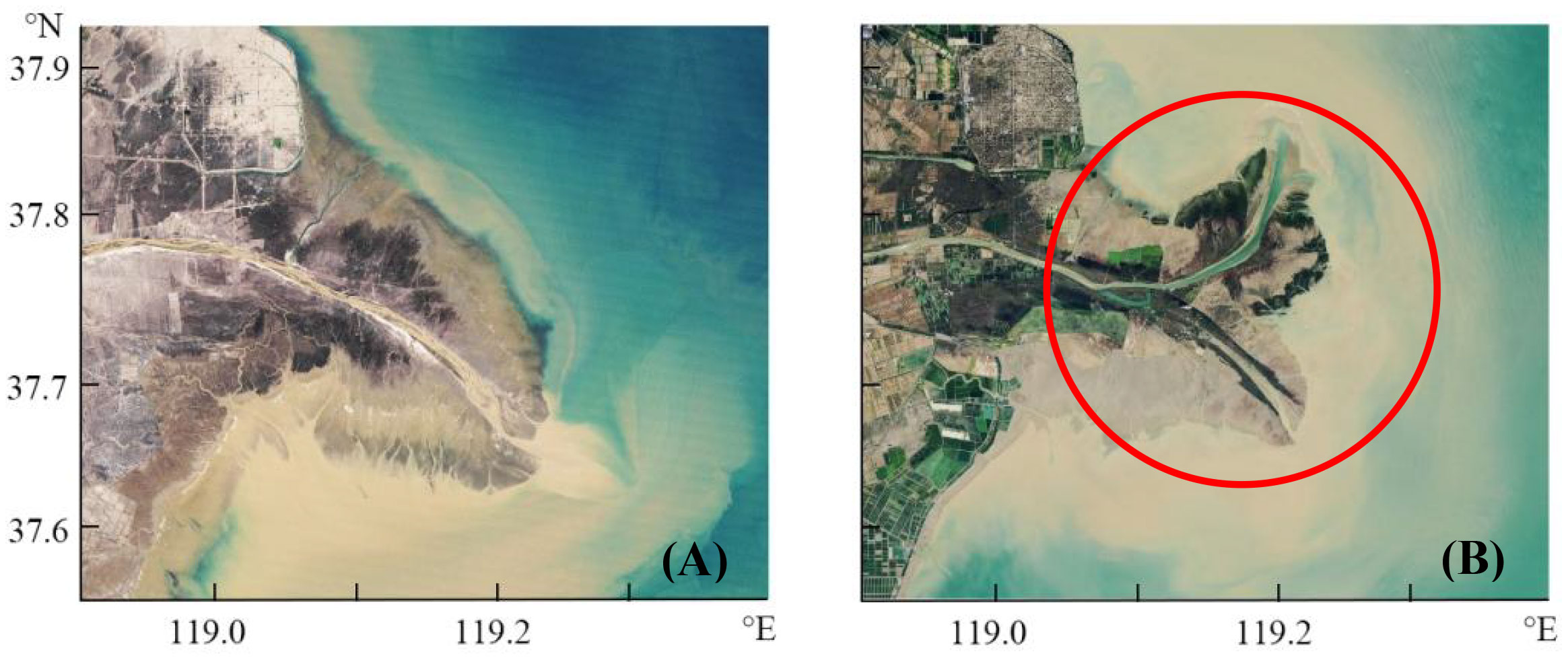
Figure 1 Landsat satellite images of the YRD in 1989 (A) and 2015 (B). (https://earthobservatory.nasa.gov/world-of-change/YellowRiver).

In the YRE, most studies have mainly focused on the changes in marine dynamics (Wang et al., 2015), sediment transport, and seabed erosion (Wang et al., 2010; Zhou et al., 2014). However, the headland-induced transport process and distribution structure in the YRE have received less attention. Here, three Lagrangian approaches—Lagrangian particle trajectories, Lagrangian residual currents, and Lagrangian coherent structures (LCSs)—are applied to study the effects of the headland on the surface material transport around the headland (red circle in B) in YRE. The first two approaches are traditional Lagrangian methods to describe long-term mass transport (Feng, 1986; Havens et al., 2010), which are unstable owing to their sensitivity with respect to initial conditions. By contrast, as a locally strongest repelling or attracting material surface (Haller and Yuan, 2000), LCSs are robust features of Lagrangian fluid motion. In recent years, LCS has been widely used to study the structures of flow fields in the ocean, atmosphere, and human blood (Nolan et al., 2019; Ghosh et al., 2021; Mutlu et al., 2021), as well as transport and mixing structures near the islands and headlands (Suara et al., 2020). In this study, the three Lagrangian approaches are combined to describe the transport and diffusion characteristics of the material in YRE.

The remainder of the paper is organized as follows: Data and methods are presented in Section 2. In Section 3, an ideal model test is performed to present the influence of the headland on the structure of material transport. Then, Lagrangian particle tracking, Lagrangian residual current, and LCS methods are applied to describe the transport of floating materials near the YRE. Sections 4 and 5 present the discussions and conclusions of this study.

2 Materials and methods

2.1 Data

The data used in this study are generated by an unstructured grid, Finite-Volume, primitive equation Community Ocean Model (FVCOM), that is well suited to simulating the circulation in regions characterized by complex irregular coastlines, islands, inlets, creeks, and intertidal areas. For more information on FVCOM, see the reference Chen et al. (2006). The modeled area in this study covers the entire Bohai Sea, and the open boundary (from Chengshantou to Dandong City) is shown in Figure 2. In the nearshore area, with the tide as the main forcing factor, the model is forced by four primary tidal constituents (M2, S2, K1, and O1) on the open boundary and freshwater. The horizontal grid resolution ranges from 200 m in the YRE to 5,000 m outside the study area, and 5 -coordinate layers are used in the vertical. The bottom roughness height is set to a constant of 0.001 m. The model is the same as the reference model (Lou et al., 2022) and has been calibrated and verified with field observations.

FIGURE 2

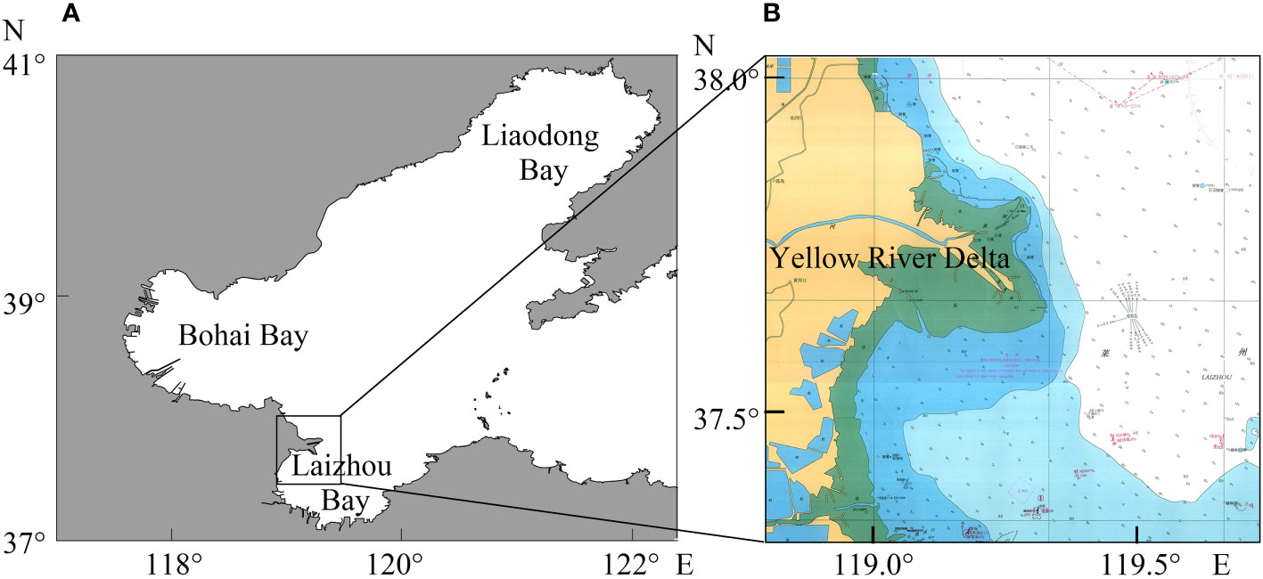
Figure 2 The topographic map of Bohai (A) and water depth in the main study area of Yellow River Delta (B).

2.2 Lagrangian description methods

2.2.1 Lagrangian particle tracking

Material transport and mixing in the ocean are governed by two fundamental physical processes (advection and diffusion). The effect of the diffusion process may be negligible over short time intervals relative to the advection timescale [t0, t1] (Hadjighasem, 2016). In this case, the trajectories of the passive tracers coincide with the trajectories of the fluid particles. Therefore, the motions of the fluid particles satisfy the differential equation:

$\begin{array}{ll}d\overrightarrow{x}/dt=\overrightarrow{v}(\overrightarrow{x}(t;t_0,x_0),t)& (1)\end{array}$

where $\overrightarrow{x}(t;t_0,x_0)$ is the particle position at time t, $d\overrightarrow{x}/dt$ the derivative of $\overrightarrow{x}$ with respect to time t, and $\overrightarrow{v}(\overrightarrow{x}(t;t_0,x_0),t)$ the flow velocity generated by the FVCOM model. A 4th order partial time step Runge–Kutta scheme was used to update the particle locations.

2.2.2 Lagrangian residual current

The Lagrangian residual current is defined as the net Lagrangian drift displacement of a marked water parcel in a tidal period Tt and divided by Tt (Cheng and Casulli, 1982). In the nearshore zone, the dynamic system is nonlinear due to seafloor friction and obstruction by the tortuous coastline. For highly nonlinear systems, numerical methods based on particle tracking can calculate the Lagrangian residual circulation. The LRC also depends strongly on the initial release time and integration time (Muller et al., 2009). The particle trajectory equation is presented in Equation (2):

$\begin{array}{ll}{\overrightarrow{u}}_{lr}(X_0,t_0)=\frac{\overrightarrow{Y}(X_0,t_0+T_t)-\overrightarrow{Y}(X_0,t_0)}{T_t}& (2)\end{array}$

where T_t is a tidal period, X₀ and $\overrightarrow{Y}(X_0,t_0)$ the location and the trajectory of the labeled fluid parcel on the horizontal plane at time t₀, $\overrightarrow{Y}(X_0,t_0+T_t)$ the trajectory at time t₀ + T_t. In this study, the tracking trajectories of particles are calculated based on flow field data calculated using FVCOM.

2.2.3 Lagrangian coherent structures

LCSs provide a new way to understand transport in complex fluid flows (Peacock and Haller, 2013). Many LCS diagnostics have been developed to detect different types of structures, among which finite-time Lyapunov exponents (FTLE) are simple and objective algorithms (Hadjighasem et al., 2017).

The FTLE is a finite-time average of the maximum expansion rate for a pair of particles advected by the flow during the period from t to t + T (Shadden et al., 2005; Peacock and Haller, 2013). The FTLE is given by:

$\begin{array}{ll}FTLE(x_0)=\frac{1}{|t_1-t_0|}\ln \sqrt{\lambda {(\Delta )}_{\max }}=\frac{1}{\left|T\right|}\ln \sqrt{\lambda {(\Delta )}_{\max }}& (3)\end{array}$

$\begin{array}{ll}\Delta ={\phi }^{*}\times \phi & (4)\end{array}$

where T is the integration length, λ(Δ)_max is the maximum eigenvalue of a symmetric matrix Δ and φ the spatial deformation gradient tensor of the motion trajectory from t to t + T, and φ* denotes the matrix transposition of φ.

The repelling LCS (rLCS) from t₀ to t₁ is a local maximization curve or peak of the FTLE. The attracting LCS (aLCS) from t₁ to t₀ is a peak of the FTLE field in back time, which can be understood as the accumulation line or the boundary of the accumulation zone during material transportation (Haller, 2001b; Haller, 2002). Using the finite-difference method with the values of neighboring grid points, the spatial gradient of the flow map at each initial grid point is obtained (Haller, 2001a; Shadden et al., 2005). The deformation gradient tensor φ in two-dimensional spaces is calculated as:

$\begin{array}{ll}\phi =\left[\begin{array}{l}\frac{x_{i+1,j}(t+T)-x_{i-1,j}(t+T)}{x_{i+1,j}(t)-x_{i-1,j}(t)}\frac{x_{i,j+1}(t+T)-x_{i,j-1}(t+T)}{y_{i,j+1}(t)-y_{i,j-1}(t)}\\ \frac{y_{i+1,j}(t+T)-y_{i-1,j}(t+T)}{x_{i+1,j}(t)-x_{i-1,j}(t)}\frac{y_{i,j+1}(t+T)-y_{i,j-1}(t+T)}{y_{i,j+1}(t)-y_{i,j-1}(t)}\end{array}\right]& (5)\end{array}$

where x and y are spatial coordinates, and i and j grid node numbers.

In this study, the code used to calculate the FTLE field was programmed in MATLAB, which is the same as that in the reference (Lou et al., 2022). In order to prove the feasibility of the code, we test the code on the time-varying double-gyre flow field, and the FTLE field at t = 0 is consistent with that by Jakobsson (2012).

The double gyre flow field is defined in a domain Ω:{x ∈ [0,2],y ∈ [0,1]} by the stream function Ψ:

$\begin{array}{ll}\psi (x,y,t)=A\sin (\pi f(x,t))\sin (\pi y)& (6)\end{array}$

$\begin{array}{ll}f(x,t)=a(t)x^2+b(t)x,a(t)=ϵ\sin (\omega t),b(t)=1-2ϵ\sin (\omega t)& (7)\end{array}$

The velocity field is:

$\begin{array}{ll}{u}_x=\frac{\partial \psi }{\partial y},u_y=-\frac{\partial \psi }{\partial x}& (8)\end{array}$

where A = 0.1, ϵ = 0.25, ω = 2π/10.

Since the instantaneous distribution of the buoyant material approximates the attracting material curves, which are related to the backward FTLE, we compared the distribution obtained from particle tracking with aLCSs. The particles are released from the red and black areas at t = 0 (Figure 3A). The particle distributions at t = 16 s, 18 s, and 20 s are shown in Figures 3B-D superimposed on the aLCSs at the corresponding times. The particles accumulate on both sides of the banded aLCSs. This indicates that the aLCSs actually act as barriers in the material transport process, making the material unevenly distributed. LCS provides a powerful method for describing transport phenomena that are not revealed by instantaneous measurements.

$$\overrightarrow{v}(t)={\overrightarrow{V}}_0·\cos \left((\pi /6)t\right)$$

FIGURE 3

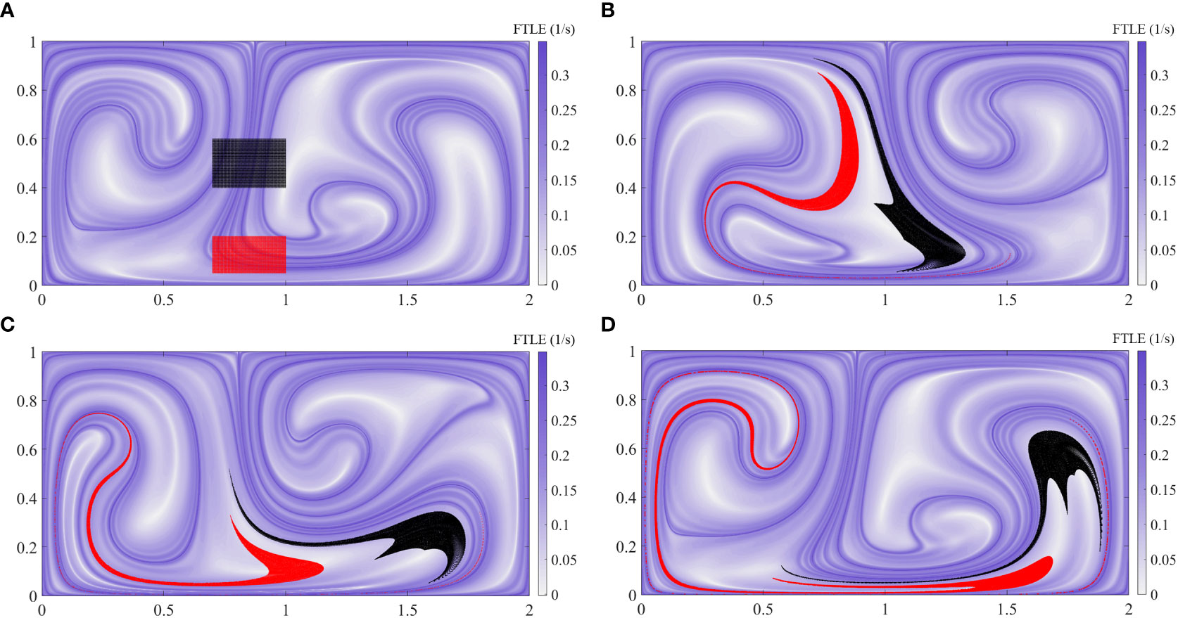
Figure 3 Plot of tracer particles injected at t = 0 s (A) and position of the particle at t = 16 s (B), 18 s (C), and 20 s (D), superimposed aLCSs at the corresponding time on the base map.

2.2.4 Idealized models

Particle tracking experiments were conducted in an ideal sea area 20 km long and 10 km wide. The model is forced by the alternating flow on the western and eastern open boundaries:

$\begin{array}{ll}\overrightarrow{v}(t)={\overrightarrow{V}}_0·\cos \left((\pi /6)t\right)& (9)\end{array}$

in which t is the time and ${\overrightarrow{V}}_0$ the amplitude of the velocity.

The model area contains a 3.5 km long and 1.75 km wide headland, and the water depth in the model is 15 m. Three experimental scenarios were set up (Figure 4), with the velocity magnitude V₀ being 0.1, 0.3, and 0.5 m/s, respectively. Particles were released during flood time after the model spin-up. On the southern and northern boundaries, reflection boundary conditions are adopted.

FIGURE 4

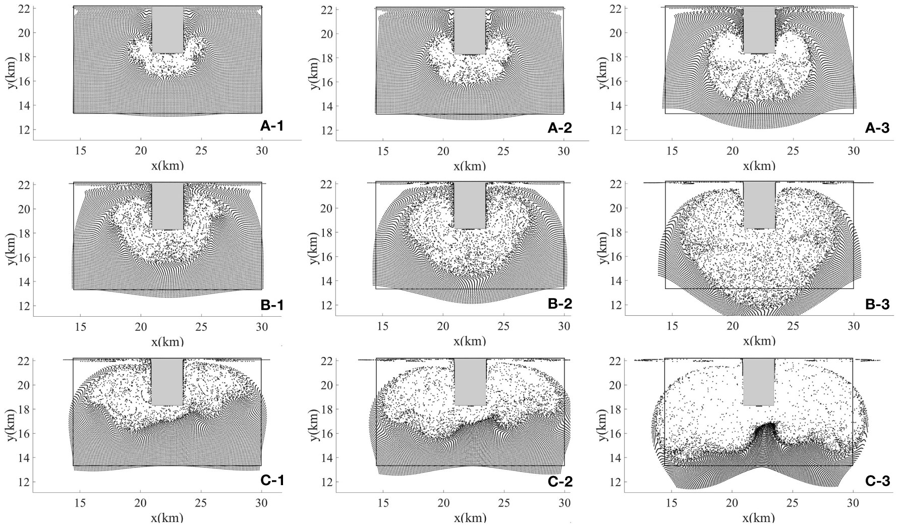
Figure 4 Particle distribution after t = 60 h (A-1, B-1, C-1), 120 h (A-2, B-2, C-2), 360 h (A-3, B-3, C-3) Under the action of three different flow velocities V0 = 0.1 m/s (A), 0.3 m/s (B), and 0.5 m/s (C),. The box with black lines is the initial release area of the particles.

3 Results

3.1 Material transport for the idealized models

The particle distribution patterns in tests A, B, and C are similar. The particles are advected by the flow around the headland, and an expansion zone with a low particle density area appears and forms a particle distribution front. After the same period, the increase in velocity causes test B to have a stronger mixing or diffusion area than test A. When the current velocity increases to 0.5 m/s (test C), the particle distribution pattern obviously changes, and the strong scattering zone extends mainly on the western and eastern sides of the headland for a longer distance and a larger area. However, particles accumulated in front of the headland, and the distance between the headland and the underlying front became shorter. When t = 360 h (Figure 4C-3), a zone of particle accumulation formed in front of the headland.

3.2 Lagrangian particles tracking

Virtual particles representing floating trash, fish eggs, larvae, phytoplankton, etc. are uniformly released in the study area. The orbits of individual particles are affected by the released time, but over several tidal periods, the effect will be weakened. Figure 5 shows the particle distribution after 300 h. Particles released at low tide and high tide showed similar results after 300 h.

FIGURE 5

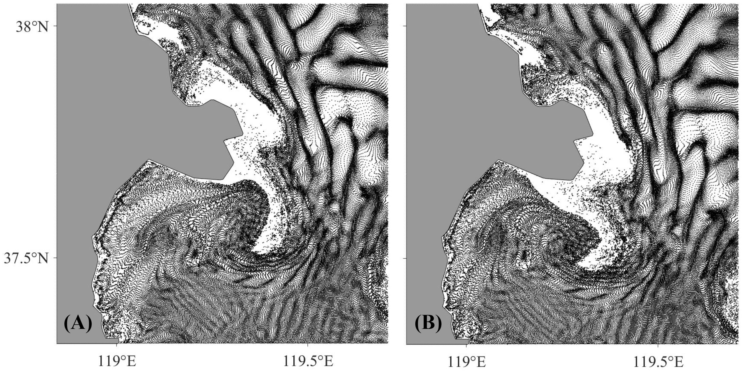
Figure 5 Particles released at low tide (A) and high tide (B), respectively, and particle distribution after 300 h.

Due to the influence of the headland and the freshwater of YR, a strong turbulent mixing or material diffusion zone (the area with few particles) appears in front of the headland, the boundary of which is about 10 km from the coast. Compared to the idealized model in Section 3.1 (see Figure 4), the material distribution structure is more similar to test C, i.e., the edge of the strong material diffusion area in front of the headland widens towards the coast. The material diffusion zone southeast of the headland is deformed into a narrow band. The boundary of the strong turbulent mixing or material diffusing zone leads to a material accumulation zone, which can be considered the front of a headland. The particle trajectory analysis method for material distribution in instantaneous time is very intuitive, but it is difficult and complex to analyze the transport process through the particle orbit.

3.3 LRC in the Yellow River Estuary

In this article, LRC is calculated by the numerical method-based Equation (3). When the particles are released at high tide, there is a clockwise LRC vortex to the south of the headland (red arrows in Figure 6B). This is consistent with the conclusion of Wang et al. (2015). If the particles are released at low tide, there is a tongue-like LRC (red box in Figure 6A).

FIGURE 6

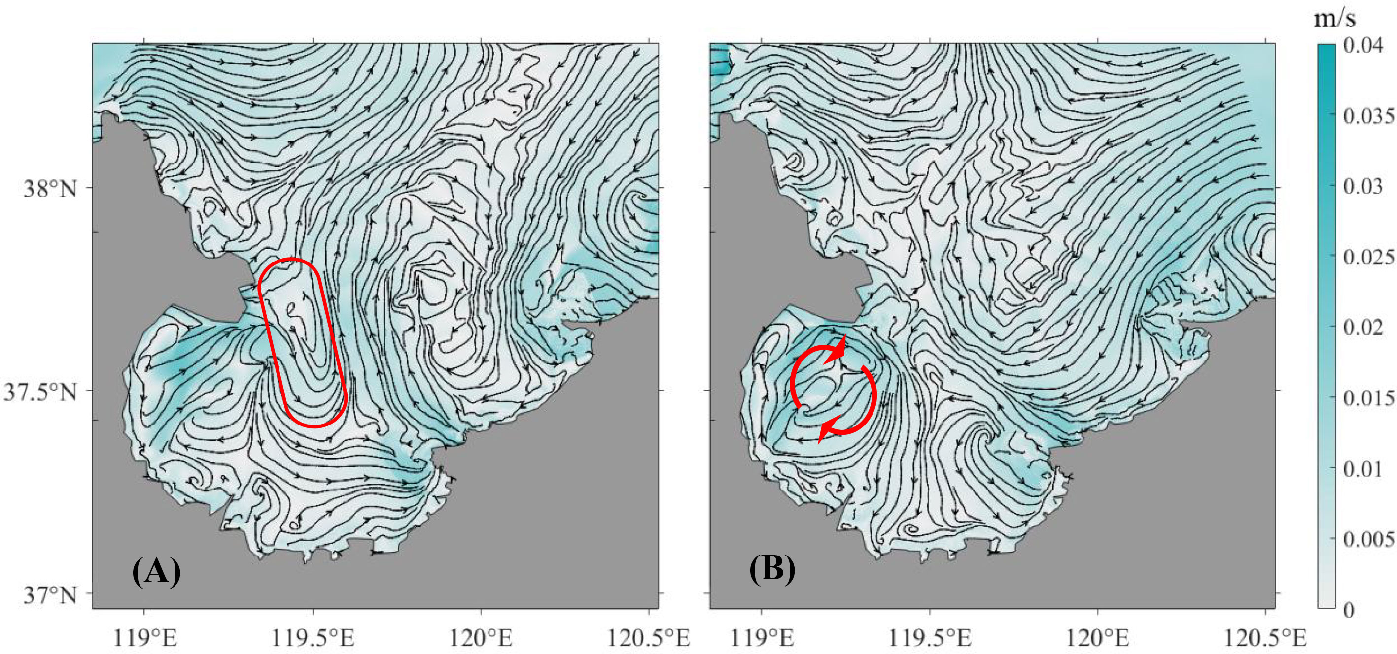
Figure 6 Lagrangian residual current velocity with respect to time t = 300 h at low tide (A) and high tide (B) in the LZB.

In general, under the influence of the headland shape drag, the turbulent eddy appears in the lee of the headland or near the headland (Figure 6). The LRC becomes a more regular coastal flow about 10 km from the headland. This indicates that there is a strong turbulent mixing zone or a material diffusion zone around the headland. This is consistent with the particle tracking results.

The structure of the LRC around the headland influences the transport of materials and reveals the pathways and accumulation zones of pollutants in Laizhou Bay (LZB). This is very useful for understanding the pollution mechanism and formulating reasonable water pollution control measures in the LZB.

3.4 LCSs in the Yellow River Estuary

The LCSs can be obtained by extracting the FTLE edge based on Formula (2), which is easily identified from the FTLE field by intuitive observation without complex LCS extraction techniques. Figure 7 shows the backward FTLE field over a 200-hour time interval, in which (A) corresponds to particles released at low tide and (B) corresponds to particles released at high tide. The two FTLE distributions are nearly consistent, suggesting that the FTLE is a more stable Lagrangian variable than either the single particle trajectory or the LRC.

FIGURE 7

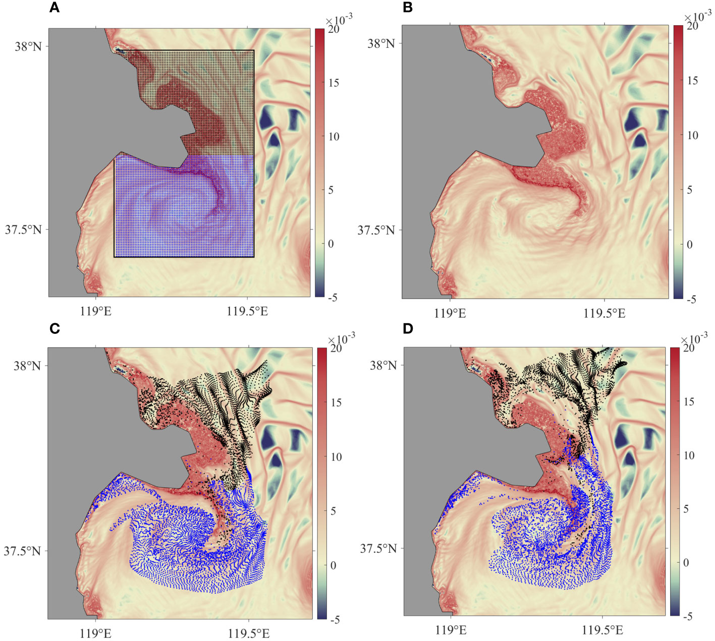
Figure 7 Particles were released at low tide and high tide in the study area, respectively, in the backward FTLE field (A) and (B) over a 200-hour time interval. Points with different colors in the box in (A) are the initial positions of the particles released on the north and south sides of the LCS. Particle distribution after 300 h (C) and 500 h (D) of release.

The ridge of the back FTLE fields (Figures 7A, B) is considered aLCSs. They are considered transport barriers and prevent material exchange between the two sides. To the southeast of the headland, there is a banded aLCS that extends eastward. This causes the material from the YR to be blocked here and then transported to the east of the bay. These structures together form the tidally induced headland front in the YRE.

To further describe the transport and distribution structure of surface materials in the YRE, particles are released into the adjacent sea area of the YRE at low tide. Particles to the north and south of the banded LCSs are marked with different colors (Figure 7A). The distribution of particles after 300 h and 500 h is shown in Figures 7C, D. It can be seen that most of the black particles, after being advected by the flow, move to the northeast and then accumulate along the aLCS. Due to the existence of aLCs and the vortex, the blue particles to the south are controlled and captured by the aLCS. Notably, as in the ideal test C, in front of the headland, the aLCS extends toward the headland, and particles are captured and accumulated there.

4 Discussion

The material transport structure near the YRE is mainly affected by the estuary shoreline and the periodically alternating flow field. Eddies are easily formed around the headland (Tang and Chen, 2012), which will capture the material such as suspended sediment and plankton to form a front or patch distribution. In this paper, an experiment has been carried out to test the effect of the headland on the circulation and transport of material in the YRE. In this experiment, the coastline in the YRE has been modified to follow a straight line, and the other parameters remain unchanged. Take the LRC at high tide as an example: without considering the headland, the clockwise circulation in the west of the LZB will disappear, but instead, a clockwise circulation will appear in the north of the LZB (Figure 8A). Due to the changed circulation structure, materials are easy to accumulate in the northwest of the LZB (Figure 8B). The LCSs results also indicate that the local barrier and pathway in the estuary will disappear without considering the headland.

FIGURE 8

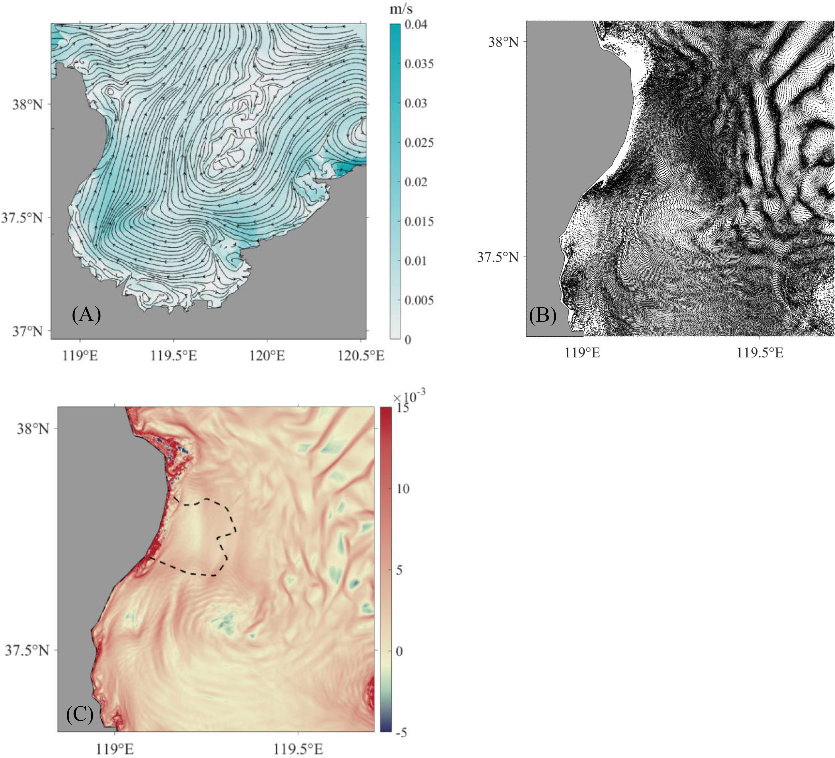
Figure 8 The Lagrangian residual current (A), particle distribution after 300 h (B), and backward FTLE field for 200 h (C) obtained from the model after adjusting the coastline at the time are consistent with the high tide in Figures 5–7.

The material transport path and accumulation area proposed in our study are consistent with existing research. Research by Huang and Su (2002) also confirms this hypothesis and shows that the transport pattern of prawn eggs and larvae has fundamentally changed after the modification of the delta shoreline. Prawn eggs and larvae outside the bay cannot enter the bay. In contrast, those to the northwest are caught in an eddy at the tip of the YRE and cannot reach the nearshore area. The research of Wang et al. (2017) on phytoplankton community structure in the YRE also supports this conclusion by providing evidence that depth-weighted phytoplankton abundance and phytoplankton biodiversity indices are high south of the YRE front. Ge et al. (2019) found that the area with high values of the zooplankton Shannon–Weaner Index (which indicates the percentage of community abundance) appeared at the front of the YRE headland. The distribution of eggs and larvae in the spring and summer horizontal features obtained by Bian et al. (2010) also showed a similar pattern.

5 Conclusions

In this article, three Lagrangian approaches are applied to describe the material transport and diffusion characteristics in the YRE. The study results indicate that LCS calculated by the ridge of the FTLE fields is a more robust description, compared to LRC and particle trajectories. But we suggest it is essential to combine these Lagrangian approaches in terms of material transport and its dynamic mechanism.

The headland is shown to play a vital role in the transport and mixing of the materials in the YRE. On the left and right sides of the headland (facing the sea), there exist a pair of clockwise or counterclockwise circulation vortices, which is the dynamical mechanism of the material transport. Due to the effect of the headland, surface materials in the YRE are distributed in patches, and an accumulation zone has formed southeast of the headland.

The pattern revealed by the Lagrangian approach is helpful for understanding the process of material transport and distribution, which has important ecological and economic implications. For example, it can be applied to predict the impact of a pollution accident. It can also provide a reference for the selection of key monitoring areas and sampling stations for water quality monitoring. In addition, it can provide guidance for the management of the marine protected area.

Data availability statement

The original contributions presented in the study are included in the articles. Further inquiries can be directed to the corresponding authors.

Author contributions

XZ proposed the idea and designed the outline of this paper, and revised the paper for meeting scientific standard. QL ran the hydrodynamic model, analyzed the data using LCS method, and wrote the paper. XX constructed the idealized models and helped to write some sentences in Section 3.1. ZC gave some useful advice that improved the quality of the paper. ZL gave some useful advice for revising the paper. All authors contributed to the article and approved the submitted version.

Funding

This work is supported by the National Natural Science Foundation of China (No. 41974085) and the National Key R&D Program of China (No. 2019YFC1408100).

Acknowledgments

The authors would like to express their gratitude to EditSprings (https://www.editsprings.cn) for the expert linguistic services provided.

Conflict of interest

The authors declare that the research was conducted in the absence of any commercial or financial relationships that could be construed as a potential conflict of interest.

Publisher’s note

All claims expressed in this article are solely those of the authors and do not necessarily represent those of their affiliated organizations, or those of the publisher, the editors and the reviewers. Any product that may be evaluated in this article, or claim that may be made by its manufacturer, is not guaranteed or endorsed by the publisher.

References

Alaee M. J., Ivey G., Pattiaratchi C. (2004). Secondary circulation induced by flow curvature and Coriolis effects around headlands and islands. Ocean Dynam. 54 (1), 27–38. doi: 10.1007/s10236-003-0058-3

CrossRef Full Text | Google Scholar

Bian X. D., Zhang X. M., Gao T. X., Wan R. J., Zhang P. D. (2010). Category composition and distributional patterns of ichthyoplankton in the yellow river estuary during spring and summer 2007. J. Fishery Sci. China 17 (4), 815–827.

Google Scholar

Chen C. S., Beardsley R., Cowles G. (2006). An unstructured grid, finite-volume coastal ocean model (FVCOM) system. Oceanography 19 (1), 78–89. doi: 10.5670/oceanog.2006.92

CrossRef Full Text | Google Scholar

Cheng R. T., Casulli V. (1982). On Lagrangian residual currents with applications in south San Francisco bay, California. Water Resour. Res. 18 (6), 1652–1662. doi: 10.1029/wr018i006p01652

CrossRef Full Text | Google Scholar

Dong C. M., McWilliams J. C. (2007). A numerical study of island wakes in the southern California bight. Continental Shelf Res. 27 (9), 1233–1248. doi: 10.1016/j.csr.2007.01.016

CrossRef Full Text | Google Scholar

Feng S. (1986). A three-dimensional weakly nonlinear dynamics on tide-induced Lagrangian residual current and mass-transport. Chin. J. Oceanol. Limnol. 4 (2), 139–158. doi: 10.1007/bf02850431

CrossRef Full Text | Google Scholar

Ge R., Liu G. X., Chen H. J., Li Z. S., Li H. R. (2019). Community characteristics of zooplankton sampled with two plankton nets in yellow river estuary in spring. Periodical ocean Univ. China 49 (4), 62–70.

Google Scholar

George D. A., Largier J. L., Storlazzi C. D., Robart M. J., Gaylord B. (2018). Currents, waves and sediment transport around the headland of pt. dume, California. Continental Shelf Res. 171 (1), 63–76. doi: 10.1016/j.csr.2018.10.011

CrossRef Full Text | Google Scholar

Ghosh A., Suara K., McCue S. W., Yu Y. Y., Soomere T., Brown R. J. (2021). Persistency of debris accumulation in tidal estuaries using Lagrangian coherent structures. Sci. Total Environ. 781, 146808. doi: 10.1016/j.scitotenv.2021.146808

CrossRef Full Text | Google Scholar

Hadjighasem A. (2016). Extraction of Dynamical Coherent Structures from Time-Varying Data Sets. McGill University, PhD Thesis. ETH Zurich. 23522. doi: 10.3929/ethz-a-010737559

CrossRef Full Text | Google Scholar

Hadjighasem A., Farazmand M., Blazevski D., Froyland G., Haller G. (2017). A critical comparison of Lagrangian methods for coherent structure detection. Chaos: An Interdisciplinary Journal of Nonlinear Science 27 (5), 053104. doi: 10.1063/1.4982720

CrossRef Full Text | Google Scholar

Haller G. (2001a). Lagrangian Structures and the rate of strain in a partition of two-dimensional turbulence. Phys. Fluids 13 (11), 3365–3385. doi: 10.1063/1.1403336

CrossRef Full Text | Google Scholar

Haller G. (2001b). Distinguished material surfaces and coherent structures in three-dimensional fluid flows. Physica. D Nonlinear Phenomena 149 (4), 248–277. doi: 10.1016/S0167-2789(00)00199-8

CrossRef Full Text | Google Scholar

Haller G. (2002). Lagrangian Coherent structures from approximate velocity data. Phys. fluids 14 (6), 1851–1861. doi: 10.1063/1.1477449

CrossRef Full Text | Google Scholar

Haller G., Yuan G. (2000). Lagrangian Coherent structures and mixing in two-dimensional turbulence. Physica. D: Nonlinear Phenomena 147 (3-4), 352–370. doi: 10.1016/S0167-2789(00)00142-1

CrossRef Full Text | Google Scholar

Havens H., Luther M. E., Meyers S. D., Heil C. A. (2010). Lagrangian Particle tracking of a toxic dinoflagellate bloom within the Tampa bay estuary. Mar. pollut. Bull. 60 (12), 2233–2241. doi: 10.1016/j.marpolbul.2010.08.013

PubMed Abstract | CrossRef Full Text | Google Scholar

Huang D. J., Su J. L. (2002). The effects of the huanghe river delta on the circulation and transportation of larvae. Acta Oceanol. Sin. 24, 104–111.

Google Scholar

Jakobsson J. (2012). Investigation of Lagrangian coherent structures-to understand and identify turbulence (Gothenburg, Sweden: Chalmers University of Technology).

Google Scholar

Lou Q., Li Z. Y., Zhang Y. W., Feng Y. L., Zhang X. Q. (2022). Impact of typhoon lekima, (2019) on material transport in laizhou bay using Lagrangian coherent structures. J. Oceanol. Limnol. 40, 922–933. doi: 10.1007/s00343-021-0384-7

CrossRef Full Text | Google Scholar

Magaldi M., Russo R., Bevilacqua L., Pierno S., Carlo V. S., Corvino F., et al. (2008). A GRID Approach to Providing Multimodal Context-Sensitive Social Service to Mobile Users. OTM Confederated International Conferences “On the Move to Meaningful Internet Systems”. (Berlin, Heidelberg: Springer). 2008, 528–537. doi: 10.1007/978-3-540-88875-8_76

CrossRef Full Text | Google Scholar

Milliman J. D., Meade R. H. (1983). World-wide delivery of river sediment to the oceans. J. Geol. 91 (1), 1–21. doi: 10.1086/628741

CrossRef Full Text | Google Scholar

Ministry of Water Resources of the People’s Republic of China (2022). 2021 China river sediment bulletin. (Beijing, China: China Water & Power Press). 20–21.

Google Scholar

Muller H., Blanke B., Dumas F., Lekien F., Mariette V. (2009). Estimating the Lagrangian residual circulation in the iroise Sea. J. Mar. Syst. 78 (1), 17–36. doi: 10.1016/j.jmarsys.2009.01.008

CrossRef Full Text | Google Scholar

Mutlu O., Salman H. E., Yalcin H. C., Olcay A. B. (2021). Fluid flow characteristics of healthy and calcified aortic valves using three-dimensional Lagrangian coherent structures analysis. Fluids 6 (203), 1–18. doi: 10.3390/fluids6060203

CrossRef Full Text | Google Scholar

Nolan P., McClelland H., Woolsey C., Ross S. (2019). A method for detecting atmospheric Lagrangian coherent structures using a single fixed-wing unmanned aircraft system. Sensors 19 (7), 1607. doi: 10.3390/s19071607

CrossRef Full Text | Google Scholar

O’Byrne M. J., Griffiths R. W., Hughes G. O. (2007). Wake Flows in Coastal Oceans: An Experimental Study of Topographic Effects. 16th Australasian Fluid Mechanics Conference, Gold Coast, Queensland, Australia, 3–7 December, 2007.

Google Scholar

Peacock T., Haller G. (2013). Lagrangian Coherent structures: The hidden skeleton of fluid flows. Phys. Today 66 (2), 41–47. doi: 10.1063/PT.3.1886

CrossRef Full Text | Google Scholar

Saito Y., Wei H. L., Zhou Y. Q., Nishimura A., Sato Y., Yokota S. (2000). Delta progradation and chenier formation in the huanghe (Yellow river) delta, China. J. Asian Earth Sci. 18 (4), 0–497. doi: 10.1016/s1367-9120(99)00080-2

CrossRef Full Text | Google Scholar

Shadden S. C., Lekien F., Marsden J. E. (2005). Definition and properties of Lagrangian coherent structures from finite-time lyapunov exponents in two-dimensional aperiodic flows. Physica. D: Nonlinear Phenomena 212 (3-4), 271–304. doi: 10.1016/j.physd.2005.10.007

CrossRef Full Text | Google Scholar

Suara K., Khanarmuei M., Ghosh A., Yu Y. Y., Zhang H., Soomere T., et al. (2020). Material and debris transport patterns in moreton bay, Australia: The influence of Lagrangian coherent structures. Sci. Total Environ. 721, 137715. doi: 10.1016/j.scitotenv.2020.137715

PubMed Abstract | CrossRef Full Text | Google Scholar

Tang F. E., Chen D. Y. (2012). Tidal flow patterns near a coastal headland. Int. J. Civ. Environ. 6, 684–92. doi: 10.5281/zenodo.1057519

CrossRef Full Text | Google Scholar

Tatematsu S., Usui S., Kanai T., Tanaka Y., Hyakunari W., Kaneko.

Google Scholar

Wang H. J., Bi N. S., Saito Y., Wang Y., Sun X. X., Zhangm J., et al. (2010). Recent changes in sediment delivery by the huanghe (Yellow river) to the sea: Causes and environmental implications in its estuary. J. Hydrol. 391 (3-4), 302–313. doi: 10.1016/j.jhydrol.2010.07.030

CrossRef Full Text | Google Scholar

Wang N., Liu G. X., Liu X. T., Wang W. M., Chen H. J. (2017). Phytoplankton community structure in the yellow river estuary and its adjacent waters in late summer 2010. Mar. Environ. Sci. 2017 (01), 48–55.

Google Scholar

Wang N., Li G. X., Xu J. S., Qiao L. L., Dada O. A., Zhou C. Y. (2015). The marine dynamics and changing trend off the modern yellow river mouth. J. Ocean Univ. China 14 (3), 433–445. doi: 10.1007/s11802-015-2764-0

CrossRef Full Text | Google Scholar

Zhou L. Y., Liu J., Saito Y., Zhang Z. X., Chu H. X., Hu G. (2014). Coastal erosion as a major sediment supplier to continental shelves: example from the abandoned old huanghe (Yellow river) delta. Continental Shelf Res. 82, 43–59. doi: 10.1016/j.csr.2014.03.015

CrossRef Full Text | Google Scholar