
95% of researchers rate our articles as excellent or good
Learn more about the work of our research integrity team to safeguard the quality of each article we publish.
Find out more
ORIGINAL RESEARCH article
Front. Mar. Sci. , 26 January 2023
Sec. Ocean Observation
Volume 9 - 2022 | https://doi.org/10.3389/fmars.2022.998970
 Marilaure Grégoire1*
 Aida Alvera-Azcaráte2
 Luminita Buga3
 Arthur Capet1
 Sorin Constantin4
 Fabrizio D’ortenzio5
 David Doxaran5
 Yannis Faugeras6
 Aina Garcia-Espriu7
 Mariana Golumbeanu3
 Cristina González-Haro7
 Verónica González-Gambau7Jean-Paul Kasprzyk8
 Evgeny Ivanov1
 Evan Mason1,9
 Razvan Mateescu3Catherine Meulders1
 Estrella Olmedo7Leonard Pons5
 Marie-Isabelle Pujol6
 George Sarbu3
 Antonio Turiel7
 Luc Vandenbulcke1
 Marie-Hélène Rio10
In this paper, satellite products developed during the Earth Observation for Science and Innovation in the Black Sea (EO4SIBS) ESA project are presented. Ocean colour, sea level anomaly and sea surface salinity datasets are produced for the last decade and validated with regional in-situ observations. New data processing is tested to appropriately tackle the Black Sea’s particular configuration and geophysical characteristics. For altimetry, the full rate (20Hz) altimeter measurements from Cryosat-2 and Sentinel-3A are processed to deliver a 5Hz along-track product. This product is combined with existing 1Hz product to produce gridded datasets for the sea level anomaly, mean dynamic topography, geostrophic currents. This new set of altimetry gridded products offers a better definition of the main Black Sea current, a more accurate reconstruction and characterization of eddies structure, in particular, in coastal areas, and improves the observable wavelength by a factor of 1.6. The EO4SIBS sea surface salinity from SMOS is the first satellite product for salinity in the Black Sea. Specific data treatments are applied to remedy the issue of land-sea and radio frequency interference contamination and to adapt the dielectric constant model to the low salinity and cold waters of the Black Sea. The quality of the SMOS products is assessed and shows a significant improvement from Level-2 to Level -3 and Level-4 products. Level-4 products accuracy is 0.4-0.6 psu, a comparable value to that in the Mediterranean Sea. On average SMOS sea surface salinity is lower than salinity measured by Argo floats, with a larger error in the eastern basin. The adequacy of SMOS SSS to reproduce the spatial characteristics of the Black Sea surface salinity and, in particular, plume patterns is analyzed. For ocean colour, chlorophyll-a, turbidity and suspended particulate materials are proposed using regional calibrated algorithms and satellite data provided by OLCI sensor onboard Sentinel-3 mission. The seasonal cycle of ocean colour products is described and a water classification scheme is proposed. The development of these three types of products has suffered from important in-situ data gaps that hinder a sound calibration of the algorithms and a proper assessment of the datasets quality. We propose recommendations for improving the in-situ observing system that will support the development of satellite products.
The Black Sea is a miniaturized version of the global ocean where the coastal and shelf zones interact with a permanent anaerobic marine zone extending from ~100 m till the bottom (~2200m) (Murray, 1991). The opening of the Bosporus Strait at the end of the Last Glacial Maximum has allowed the intrusion of the saline Mediterranean waters transforming the Black Sea from an enclosed freshwater lake to a permanently stratified basin (Degens and Ross, 1972). The Black Sea vertical salinity profile shows the presence of a permanent halocline located between 50-150 m that significantly reduces the vertical circulation and ventilation mechanisms. Only the upper layer is seasonally oxygenated by winter cooling and mixing that transport cold well-oxygenated waters to the depth of the main pycnocline. This forms a cold-water layer, the so-called Cold Intermediate Layer (CIL). The Black Sea CIL is located between 50-100m and is characterized by a temperature below 8°C (e.g., Stanev et al., 2003). Waters below ~100-150m are essentially stagnant and have a residence time of several hundreds of years (Buesseler et al., 1991).
The Black Sea is a dilution basin with a net freshwater flux associated with precipitation and river discharges exceeding that of evaporation. Its surface layer has a salinity ranging from less than 16 psu in Regions Of River Influence (ROFI) up to 18.6-18.8 psu in the open sea. The water and salt budgets are equilibrated at the Bosporus by a net water outflow flowing at the surface and an inflow of saline Mediterranean waters flowing at depth. The main feature of the Black Sea general circulation is characterized by the presence of a basin scale cyclonic current, the Rim current, that flows along the coast with a width between 40-60 km and a speed of 0.3-0.5 ms-1 (e.g., Stanev, 1990; Oguz et al., 1992) (Figure 1). The Rim current separates circulation patterns of different length scales: the central part is occupied by a number of cyclonic gyres of a few 10-100 kms while semi-permanent small scales eddies are present on the periphery between the coast and the Rim current. The mean baroclinic Rossby radius in the basin is around 20 km, and up to 5 times lower in the shelf area on the north and eastern part of the basin (Kurkin et al., 2020). Several papers have investigated the mesoscale dynamics in the Black Sea (e.g. Staneva et al., 2001; Kubryakov and Stanichny, 2015; Bouzaiene et al., 2021).
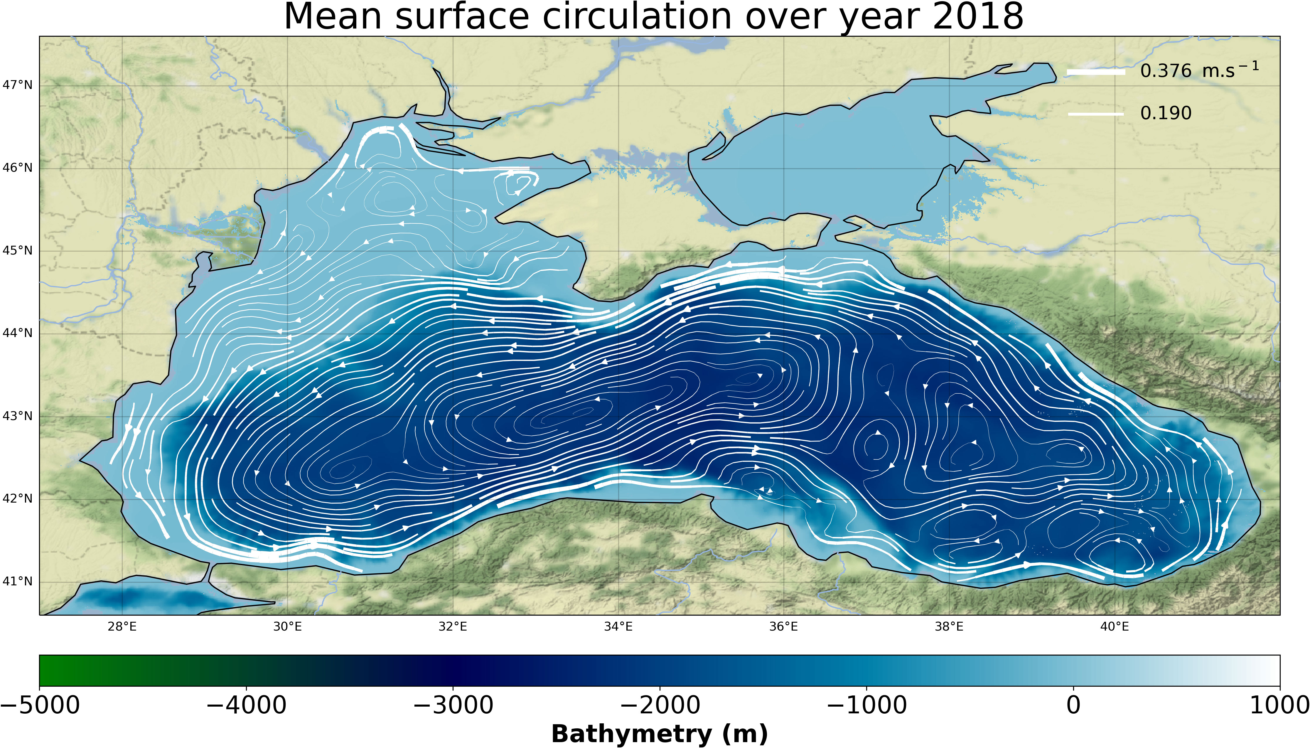
Figure 1 The Black Sea annual averaged circulation (for 2018) obtained with EO4SIBS altimetry products.
Due to its reduced size and limited lateral connections, the Black Sea is particularly sensitive to changes in its forcings (rivers, atmosphere exchanges) and is then an excellent laboratory to detect climate change and environmental impact (e.g., Grégoire and Lacroix, 2001; Oguz et al., 2006). During these last decades, signals of warming and deoxygenation have been evidenced (e.g., Konovalov and Murray, 2001; Oguz et al., 2006; Capet et al., 2016; Miladinova et al., 2017; Stanev et al., 2019; Capet et al., 2020). The formation of the CIL is becoming intermittent with years without CIL formation resulting in its progressive disappearance (e.g., Capet et al., 2014; Akpinar et al., 2017; Miladinova et al., 2017; Stanev et al., 2019; Capet et al., 2020). The reduction in CIL formation combined with intense eutrophication in the 1980s resulted in a rise of the oxycline and a significant reduction of the oxygen content of the deep sea (Konovalov and Murray, 2001; Capet et al., 2016).
The Black Sea configuration and environmental characteristics challenge the development of earth observation products from space and require the development of specific data treatments. Its moderate size and almost enclosed character make that a large fraction of the basin influenced by the coast. From the satellite data processing point of view the measurements can be strongly degraded by land-sea contamination that may induce strong biases close to the coast and affect the quality of signal corrections (Oguz and Ediger, 2006; Olmedo et al., 2021; Pujol et al., 2022). Black Sea waters are optically complex, merging large amounts of Colour Dissolved Organic Matter (CDOM) (Organelli et al., 2017) and other optically active organic and mineral Suspended Particulate Matter (SPM) delivered by its large rivers. Several regional algorithms have been developed for Chl-a (e.g., Kopelevich et al., 2002; Volpe et al., 2007; Kajiyama et al., 2018) while for SPM and Turbidity (TURB), only products obtained with global algorithms are available in operational mode. Previous endeavours related to calibration of a regional turbidity algorithm in the Danube Delta coastal area (Constantin et al., 2016) focused on MODIS imagery. As concerns Sea Surface Salinity (SSS), so far, there is no dedicated satellite-sea surface salinity (SSS) product in the Black Sea. In this paper, we present new algorithms and products developed in the frame of the 2-year ESA project EO4SIBS (Earth Observation for Science and Innovation in the Black Sea). During EO4SIBS, Ocean Colour (OC), altimetry and SSS products are produced by improving and developing algorithms and data processing to appropriately tackle the Black Sea’s particular configuration and geophysical characteristics. These products are developed for the last decade and are validated with regional datasets. They are developed aiming at better characterizing the Black Sea mesoscale and coastal processes, basin scale productivity and SSS.
The paper is organized as follows. The technical developments in terms of data processing and validation procedures are presented in Sect. 2. The products are described, and their quality assessed in Sect. 3. The complementarity and adequacy of developed products to assess the Black Sea state and variability are presented in Sect. 4. The main outcomes are summarized in Sect. 5 and recommendations for an integrated observing system combining satellite and in-situ platforms are proposed.
EO4SIBS products are summarized in Table 1 and are available from a web interface (http://www.eo4sibs.uliege.be/, Supplementary S1) and at Zenodo (Grégoire et al., 2022) under data doi: 10.5281/zenodo.6397223 with a full documentation that includes Products User Manuals (PUM) and Algorithm Theoretical Basis Document (ATBD). All these products are distributed in netCDF files.
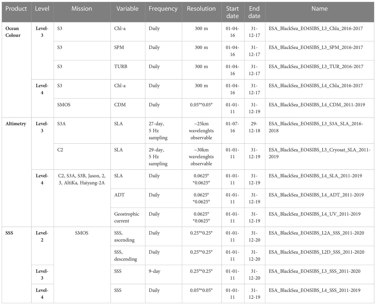
Table 1 List of products and their characteristics presented in this paper.
In this section, we overview the algorithms used to retrieve the satellite products, including the new developments and the calibration/validation procedures.
The processing used for Level-3 altimeter products is derived from the DUACS (Data Unification and Altimeter Combination System) processing currently used in the Copernicus Marine Service processing chain for the production of the Level-3 product over the Black Sea and described in Pujol et al. (2016, 2022). Here, in order to better resolve the smaller scale signal, we process the full rate Level-2 (20Hz) altimeter measurements from the Cryosat-2 (C2) and Sentinel-3A (S3A) altimeter missions to deliver a Level-3 altimeter product defined with a nearly 1 km sampling (instead of ~7 km with a conventional low resolution 1Hz measurements). This is made possible by recent advances in the altimeter technology and processing. The SAR technology available on C2 and S3A missions, as well as innovative retracking methodologies (e.g., Moreau et al., 2021) contribute to significantly reducing the measurement errors at short wavelengths. Details on the altimeter standards, applied corrections, measurements selection, cross-calibration, noise reduction and filtering are provided in Supplementary S2).
Level-4 products are produced from the 5Hz along-track altimeter products described above and from 1Hz Level-3 products from contemporaneous missions (Jason-2, Jason-3, SARAL-AltiKa, HaiYang-2A) made available in the Copernicus Marine Service (DT-2018 standards, Taburet et al., 2019). The processing applied is derived from the conventional DUACS optimal interpolation processing (e.g., Le Traon et al., 1998; Pujol et al., 2016; Taburet et al., 2019) with optimization of specific parameters to better estimate the mesoscale and coastal signal. The correlation scale function used in optimal interpolation processing is modified in order to include a bathymetry constraint (e.g., Davis, 1998; Dussurget et al., 2011; Escudier et al., 2013) and thus to better align the topographic structures with the bathymetric gradients. Additionally, eddies propagation velocities, deduced from the Copernicus Marine Forecasting Center for the Black Sea physics (Ciliberti et al., 2021) are also taken into account in the correlation scale definition (Supplementary S2). Finally, the SLA signal is interpolated on a regular Cartesian grid with a 0.0625°*0.0625° spatial resolution and a daily sampling. Absolute Dynamic Topography (ADT) and geostrophic currents are also estimated adding to the SLA, the regional Black Sea Mean Dynamic Topography (MDT) available on the Copernicus Marine Service Sea Level Thematic Assembly Center SEALEVEL_BLK_PHY_MDT_L4_STATIC_008_067 product (Mulet et al., 2021).
Over the last decades, numerous algorithms for atmospheric corrections were proposed, validated and implemented in operational procedures (e.g., Goyens et al., 2013; Novoa et al., 2017; Renosh et al., 2020). In order to select the most suitable solution for the retrieval of remote sensing reflectance (Rrs), algorithms adapted to clear and optically complex waters are tested. The widely used POLYMER (i.e., POLYnomial based algorithm applied to MERIS) algorithm (Steinmetz et al., 2011), BAC (i.e., Baseline Atmospheric Correction) that is used by EUMETSAT for processing the standard Level-2 OLCI products (Antoine and Morel, 1999; Moore et al., 2017), and C2RCC (i.e., Case 2 Regional CoastColour) based on neural network and designed to improve radiometric parameters estimation in complex waters (Doerffer and Schiller, 2007) are compared. The quality of these algorithms is assessed by comparing the spectral reflectance (Rrs) retrieved from S3 OLCI using different atmospheric corrections with that measured in the field by the two Black Sea Aeronet-OC stations i.e., Gloria (25/01/2011-07/03/2018) and Galata (12/04/2014-31/10/2018). All available match-ups from 2017 are taken into consideration. These two stations are located in the western part of the basin relatively close to the coastline (app. 22-23 km) and are representative of different optical conditions (e.g., Gloria is sometimes exposed to the Danube River plume).
Another important aspect concerning data processing refers to the flagging scheme used. As suggested by the latest EUMETSAT report on S3 OLCI L2 collection 3 (EUMETSAT, 2021), the ANNOT flags are not considered. ANNOT_DROUT, which detects anomalously bright waters, tends to remove valid pixels in case-2 (complex) waters or if coccolithophore blooms are present. Since coccolithophores blooms are common in the Black Sea (e.g., Kubryakov et al., 2019; Kubryakova et al., 2021), it was decided not to remove these areas from subsequent analysis.
Black Sea waters are regionalized based on their optical properties. A combination of the classification methods proposed by Morel and Bélanger (2006) and Dogliotti et al. (2015) is used to distinguish 3 classes of water masses differentiated by the nature of the dominant active optical constituents. The so-called case-1 waters are dominated by optically active components that are correlated to Chl-a and hence the absorption and scattering coefficients of case-1 are empirically (non-linearly) linked with Chl-a. Case-2 waters is a mixture of Chl-a, CDOM, mineral sediments (typical of coastal waters). The transition from case-1 to case-2 waters is based on the method developed by Morel and Bélanger (2006), which compares the Chl-a concentration with remote sensing reflectance values at 560 nm. Case-3 waters, introduced as a supplementary class for the Black Sea scenario, differ essentially from case-1 and case-2 by the presence of additional particles, mainly of mineral nature, and hereafter collectively called sediments (e.g., mud, sand, silt, carbonate). This is similar to the case-2S water type mentioned by Morel and Bélanger (2006). Even if they are weakly coloured and absorb the light, these particles enhance the reflectance over the whole spectrum through increased scattering. Here, case-3 waters are defined where Rrs at 665 nm is above a specific threshold (i.e., 0.0125 sr-1) empirically determined by inspection of multiple images to properly characterize the limit of the very turbid waters (especially the river plumes).
Each OC product is estimated using an approach that merges two distinct algorithms adapted to low and high values of the retrieved variable. The final product is then obtained by combining these two products according to specific thresholds and using an interpolation scheme over an overlapping range. This combination is expected to offer a more accurate retrieval over broader ranges of concentrations. For the three biogeochemical variables of interest (i.e., Chl-a, SPM and TURB), the algorithms are calibrated regionally using in-situ data when available. For Chl-a, in-situ measurements are available only for the low-end part of the concentration spectrum. Thus, for the low Chl-a regions, a blue-to-green ratio approach is adapted regionally (n=31, R=0.91, Root Mean Square Difference (RMSD)=0.17 and median absolute percentage difference (MAPD)=20.33%). A fourth-order polynomial relationship (OC4-type) between Chl-a and the maximum band ratios of reflectance at 490 nm and 510 nm with that at 560 nm is developed. For the high Chl-a regions (i.e. Chl-a > 2 mg m-3), the development of a regional algorithm is not possible due to the limited number of available in-situ datasets for its calibration and validation during the period of Sentinel data acquisition. We then use the neural network algorithm (C2RCC) including during coccolithophores blooms. C2RCC computes the absorption by phytoplankton pigments (apig) at 442.5 nm, based on the water-leaving reflectance and then links apig to Chl-a using predefined scaling factors (EUMETSAT, 2021). A merging scheme combines then results from OC4-type and C2RCC algorithms.
TURB and SPM products are retrieved using the regional adapted equations of the algorithms described in Nechad et al. (2009, 2010). These algorithms estimate TURB/SPM in relatively clear and moderate turbid waters using the water leaving reflectance in the red part of the electromagnetic spectrum (λ = 665 nm) while for turbid regions the near infrared (NIR) spectral region is used (λ = 865 nm). For the transition zone, the switch between red and NIR based algorithms is performed through linear interpolation, similar to the approach used by Dogliotti et al. (2015). This regional re-parametrization of existing approaches allows more accurate retrieval of the biogeochemical parameters. It should be noted that the application of the C2RCC algorithm for SPM estimation product, distributed together with the standard Level 2 OLCI products significantly overestimates the SPM concentrations (i.e. mean ratio between predicted and observed SPM of 2.7).
All in-situ samples available during Sentinel data acquisition are used to calibrate the OC algorithms. However, the scarcity of in-situ measurements does not allow an independent validation exercise.
Level-4 (gap-free) Chl-a products are obtained using DINEOF (Data Interpolating Empirical Orthogonal Functions, Beckers and Rixen, 2003; Alvera-Azcárate et al., 2005). DINEOF infers the missing information (e.g., due to the presence of clouds, dust or smoke in the atmosphere) thanks to a spatio-temporal analysis of the available data using an Empirical Orthogonal Functions (EOFs) basis extracted from the data themselves. Given the large size of the datasets, a separate analysis for 2016 and 2017 is realized. A first DINEOF run is performed on each of these datasets and the EOFs retained are used to detect and remove outliers, following Alvera-Azcárate et al. (2012). The final DINEOF reconstruction is done using 4 and 5 EOFs for respectively 2016 and 2017 respectively. DINEOF provides a cross-validation error estimate of the reconstruction, by masking ~3% of the initially available data in the form of clouds (see Beckers et al., 2006). The reconstruction cross-validation error is 1.35 mg m-3 for 2016 and 1.3 mg m-3 for 2017.
Level-2, Level-3 and Level-4 SMOS SSS datasets are generated starting from the brightness temperature derived from the SMOS Level-0 data. The complete description of the algorithms as well as the quality assessment of the resulting Level 3 SMOS SSS products are provided in Olmedo et al. (2022). Here, we briefly summarize the main improvements introduced from the data processing point of view for taking into account the Black Sea’s particular geographic and geophysical conditions and we refer to Olmedo et al. (2022) for further details.
Nodal sampling technique is used to reduce artefacts in brightness temperatures due mainly to Radio Frequency Interference (RFI) sources (Oliva et al., 2016) contaminations. The nodal sampling has been demonstrated to be an effective method for mitigating ripples and tails caused by RFI sources and other strong brightness temperature transitions (González-Gambau et al., 2016). This technique consists in sampling the brightness temperature at nodal points, defined as points where the contamination vanishes and the geophysical signal presents its minimum distortion. This algorithm has been enhanced by including a sea-land mask with the aim at mitigating a residual contamination that persisted in the first ~75 km close to the coast (Olmedo et al., 2022).
SSS is retrieved from measured brightness temperature and SST by using a dielectric constant model. However, the sensitivity of the brightness temperature to salinity variation decreases in cold and fresh waters leading to a significant decrease in the accuracy of the retrieved salinity. Also, the dielectric constant model performs very well in retrieving the SSS values typical of the open ocean, namely 32-38 psu, while over 15-20 psu the parameterization is not adapted, resulting in poor model accuracy. The Black Sea and, in particular, its northwestern shelf, combines low salinity (i.e., < 15 psu in the ROFI regions) and, in winter, low temperature (i.e., < 5°C with, in some regions, the presence of sea ice) waters which requires the adaptation of the dielectric constant model. Here, we use the dielectric constant model presented in González-Gambau et al. (2022). This model is proposed for the satellite salinity retrieval in the Baltic Sea that presents very low SSS and SST values. The model consists of a linear extrapolation of the algorithm presented in Meissner and Wentz (2004) for salinity values lower than 20 psu. The proposed linear extrapolation is as a function of salinity while the non-linear dependency on SST is kept unchanged.
Systematic and random errors affect the retrieval of satellite SSS. The systematic errors are separated between those errors that depend on the acquisition conditions but not on time, and those that depend on time but not on the acquisition conditions. The first ones are mainly due to land-sea contamination (Martín-Neira et al., 2016) and permanent sources of RFIs. We use the debiased non-Bayesian (dnB) approach described in Olmedo et al. (2017) to mitigate systematic biases in Level-2, Level-3 and Level-4 SSS products. The original dnB method has been developed for the global ocean and consists in estimating the biases for constant acquisition conditions (i.e., latitude, longitude, across-track distance, incidence angle, satellite overpass direction). The application of the dnB method to the Black Sea highlights spatial and temporal signals, attributed to changes in the RFI contamination and the SST values, that need to be removed. As described in González-Gambau et al. (2022), the original dnB method is extended to consider a dependency on the SST when estimating the systematic bias. Besides, since the contamination by RFI sources in 2011-2015 is different from that in 2016-2020, the systematic biases in these two periods are characterized and corrected separately.
Time dependent bias is corrected by imposing that the global ocean averaged SSS retrieved with the current algorithm does not change in time (see Olmedo et al., 2021 for the assessment of this hypothesis).
In order to mitigate the RFI contamination over the brightness temperatures, we use multifractal fusion algorithm (Umbert et al., 2014) applied to the brightness temperature data. This is the first time that multifractal fusion is applied to brightness temperatures. In previous SMOS SSS products as in Olmedo et al. (2018, 2021), multifractal fusion was applied to the Level-3 SSS leading to a new Level-4 SSS product with enhanced accuracy and resolution (Olmedo et al., 2016). In the case of the Black Sea, we need to apply the method to the brightness temperatures for obtaining Level-3 products of enough quality. Doing this, we improve the accuracy of the retrieved salinity (Olmedo et al., 2022).
We apply multifractal fusion algorithms (Umbert et al., 2014) to generate the Level-4 product as done in Olmedo et al. (2021).
The quality of the SMOS SSS products is estimated by using the correlated triple collocation method developed by González-Gambau et al. (2020). The method compares three datasets that resolve similar spatial scales, with two of them affected by correlated errors. Here, the two error correlated data sets are the different Level SSS products while the uncorrelated one is the Black Sea physical reanalysis system (version E3R1) freely distributed by the Copernicus Marine Service with the identifier BLKSEA_MULTIYEAR_PHY_007_004 and doi https://doi.org/10.25423/CMCC/BLKSEA_MULTIYEAR_PHY_007_004.
A flagging is defined for the SSS products (Level-2, -3 and -4) based on the range and variability of the products as described in Olmedo et al. (2022).
The quality of EO4SIBS satellite products is assessed and compared with in-situ data and reference products (e.g., other satellite products, model results).
The number of valid measurements and the variance of the signal increase when using the EO4SIBS 5Hz Level-3 product compared to the 1Hz product delivered by CMEMS (Figure 2 and Supplementary S2). Over the basin and, in particular, in regions close to the coast (i.e., up to 50 km away from the coast), the number of valid measurements is globally higher when considering the 5Hz altimeter product rather than the 1Hz product. It is nearly twice at ~15km from the coast and when getting closer to the coast, it drastically decreases at 1Hz while at 5Hz, even if a reduction is observed, the availability rate still remains significant up to ~5 km to the coast.
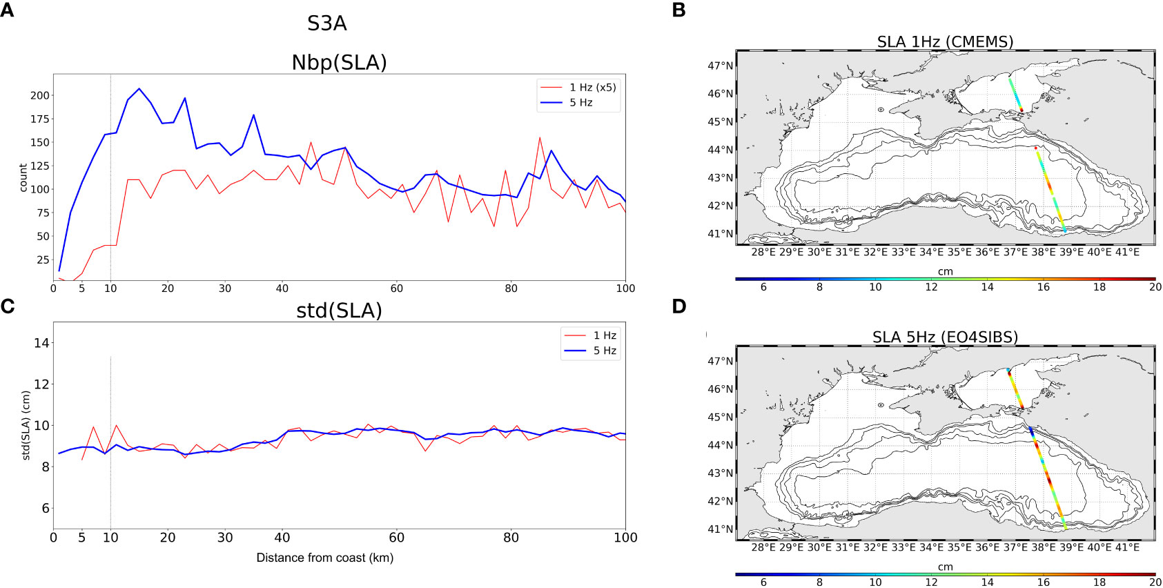
Figure 2 Left: Number of valid measurements (A) and mean SLA variance (C) as a function of the distance to the coast. Statistics computed on S3A measurements from 1Hz (red line) and 5Hz (blue line) products. Only measurement points with a minimal sampling rate of 80% compared to the maximal number of expected cycles are considered. The number of valid 5Hz measurements is divided by a factor 5 before comparison with the 1Hz product. Statistics computed over the Black Sea. Right: Example of SLA along a S3A track (date 2017/07/03) for 1Hz CMEMS product (B) and EO4SIBS 5Hz product (D).
The 5Hz measurement globally contributes increasing the spatial and temporal variance of the SLA signal by 10 to 20% (Supplementary S2). The temporal variability of the signal remains consistent between the 5Hz and 1Hz products up to ~15km (Figure 2). Closer to the coast, the variability observed with the 1Hz product shows two peaks that can be interpreted as errors in the altimeter measurement. At the opposite, the variability observed with the 5Hz product is homogeneous and consistent up to ~1km from the coast, underlining the pertinence of the additional observations brought by this product in the coastal area. This is not surprising since the 5Hz product better samples the sea surface and is specifically processed to better resolve the small wavelengths. An example of the SLA along a track is given on Figures 2B, D. It shows the improved sampling of the surface and the higher intensity of the topographic structures observed with the 5Hz product. In the eastern part of the basin, the gain of measurements with the 5Hz product is higher (Supplementary S2) mainly due to the increased availability of short segments near the coast, not present in the 1Hz product. These differences explain the high gain in SLA variance (~+40%) observed both for C2 and S3A (Supplementary S2).
The Level-4 gridded EO4SIBS product is compared to the contemporaneous Copernicus Marine Service product (regional Europe in DT-2018 version, Taburet et al., 2019). The main differences are observed in Eddy Kinetic Energy (EKE). The EKE differences (Figure 3) underscore both the coastal areas, and the continental slope with higher EKE observed in the 5Hz product. Main part of this additional energy is explained by the bathymetric constraint processing. It leads to a better definition of the Rim current characterizing the circulation in the Black Sea basin, and a more accurate reconstruction of the eddies structures in coastal areas where it contributes to close eddies contours as illustrated in Figure S2.4 in the Supplementary S2. Near the coast, the improved data availability, and thus signal observability, offered with 5Hz along-track product (S3A and C2), also contributes to this result.
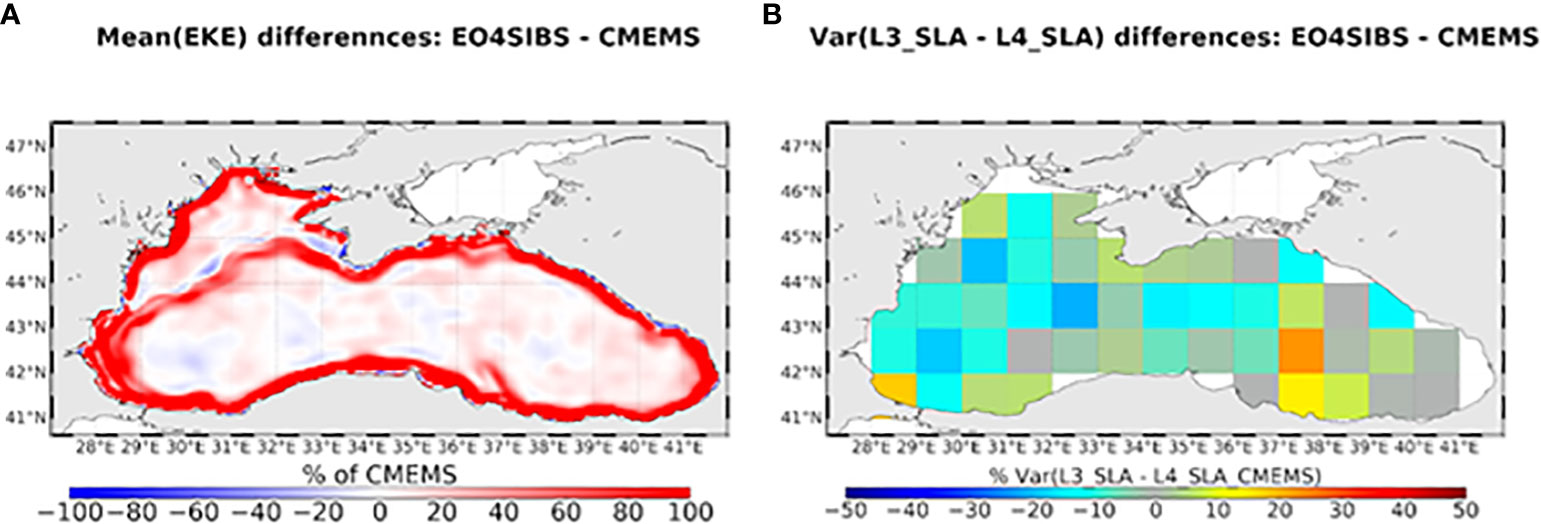
Figure 3 (A) EKE differences between EO4SIBS and CMEMS gridded products; unit: percent of the EKE from CMEMS product. (B) Difference of the variance of the gridded SLA minus along-track SLA, using successively EO4SIBS and CMEMS (DT-2018) SLA gridded products. Negative values mean that the variance of the SLA differences are reduced when considering EO4SIBS regional gridded products. The results are presented in percent of the variance of the differences between CMEMS gridded and SARAL/AltiKa along-track SLA products (white regions mean no data).
The gridded altimeter product is validated by comparison with independent measurements. Two specific map series are constructed keeping measurement from one satellite (here SARAL/AltiKa with 1Hz resolution from the Copernicus Marine Service) apart for validation purposes. They correspond to the regional product presented in this paper, and conventional regional product available from the Copernicus Marine Service. The independent measurements are here considered as a reference for mesoscale validation assuming that this signal is better observed on raw along-track measurement than on the gridded product. The latter indeed induces a smoothing of the signal. The map series that maximizes the reduction of the variance of the SLA difference between the gridded product and independent along-track is thus considered as the best map series for mesoscale observation. Figure 3B shows the results obtained over year 2017. It underscores a net reduction of the variance of the differences between gridded SLA and SARAL/AltiKa along-track SLA products when EO4SIBS grids are considered. The reduction reaches between 10 to 20% in the main part of the basin, except in the Eastern part where the Copernicus Marine products have better performances. The results also suggest a light degradation along the Crimean and southern coasts.
The comparison of the spectral water-leaving reflectance estimated from S3 OLCI using the BAC, Polymer and C2RCC algorithms for atmospheric corrections with that measured in-situ at Aeronet-OC stations shows that Polymer and BAC give better agreement than C2RCC (Supplementary S3). Overall, the error statistics (e.g., bias, RMSD, correlation) associated with Polymer and BAC are similar. Polymer performs slightly better than BAC for the blue wavelengths, but exhibits a tendency to underestimate water-leaving reflectance in the other spectral bands. The BAC algorithm for atmospheric correction, i.e. the standard Level-2 product delivered by EUMETSAT as operational and which showed satisfactory results in turbid coastal waters (Renosh et al., 2020), is selected here for further analyses. The comparison with in-situ data of the S3 OLCI retrieved SPM and TURB shows that the use of a regional algorithm improves the quality of the products with respect to a generic one (see Figure 4 for SPM). The use of two spectral bands (i.e., λ = 665 nm and λ = 865 nm) and the calibration of the algorithm’s parameters with regional data improve the quality of the product compared to an approach that uses a single spectral band (λ = 665 nm). The RMSD is reduced from 7.26 to 1.93 g m-3 while the MAPD is reduced from 35.15 to 15.89% when using a regionally fitted algorithm. The improvement is particularly visible for high SPM values. This is due to the better performance of the NIR band for these high SPM concentrations, for which the red band tends to saturate and gives false estimations. The merging scheme used in all the regional algorithms assured smooth transitions, without the presence of artificial steep gradients.
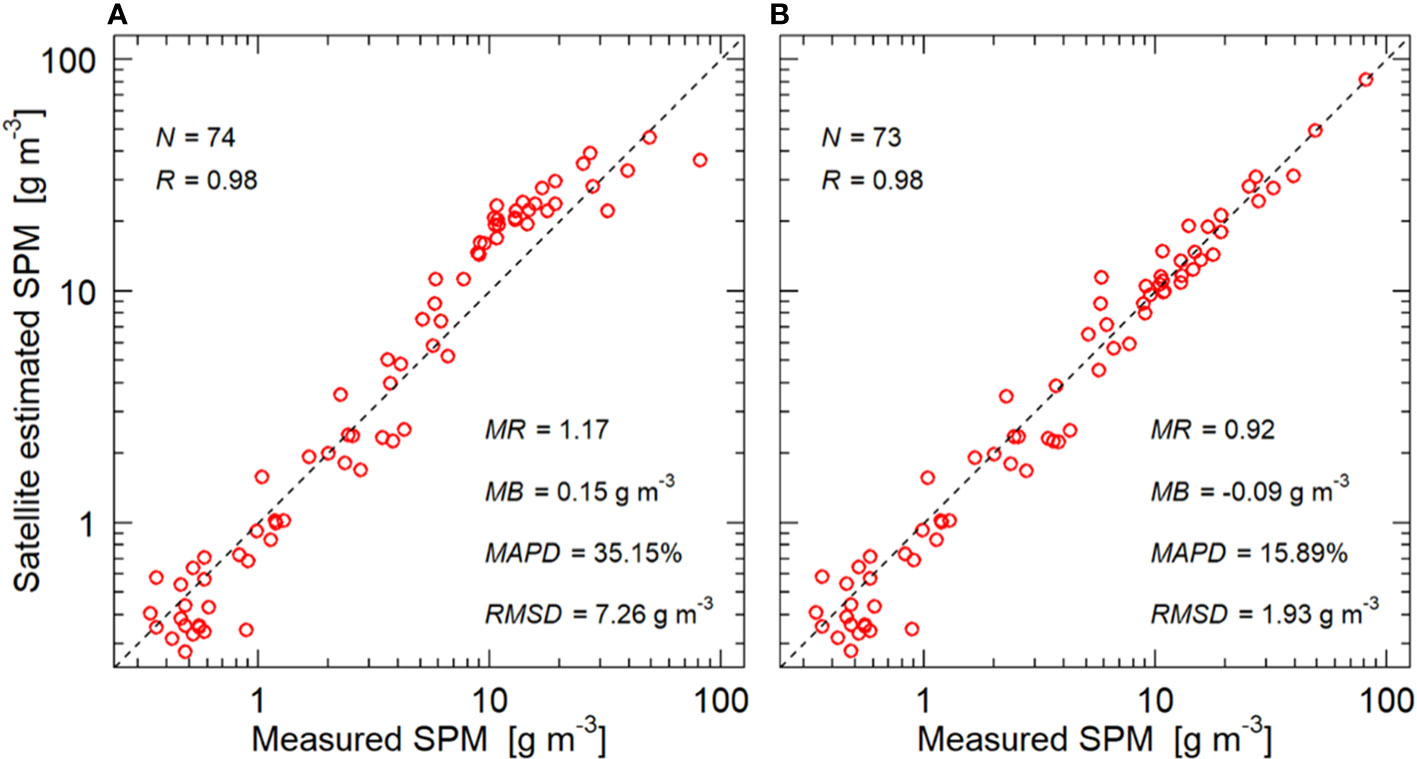
Figure 4 Scatter plot between measured and satellite-derived SPM concentrations; (A) based on the default Nechad et al. (2010) approach, using one single spectral band (λ = 665 nm); (B) based on regional adapted algorithm, which implies the usage of two spectral bands (λ = 665 nm and λ = 865 nm); N is the number of match-ups, R - the correlation coefficient, MR - median ratio between observed and predicted, MB - median bias, MAPD - median absolute percentage difference and RMSD - root mean square difference.
The comparison of the satellite-derived in-situ or modeled SSS is challenged by the fact that these estimations are obtained at different depths within the first 10 m of the water column. The topmost in-situ measured or modeled SSS, referred to as bulk SSS, is at depths larger than 1 m and mostly between 2-10 m while the satellite retrieved SSS represents the salinity in a thin layer (~1-2 cm), the skin salinity, over which the microwave radiation is penetrating. The skin SSS can be affected by evaporation-precipitation with opposite effects: precipitation dilutes the skin surface while evaporation causes skin salinification. In ROFI regions, the presence of a halocline at shallow depth (i.e. <= 10 m), decouples the skin surface from waters below the pycnocline and prevents a straightforward comparison between the satellite and in-situ SSS. In addition, sampling error (or representation error) can also be significant especially in coastal areas where this error may amount 0.4-0.7 psu (e.g., Vinogradova et al., 2019). Nevertheless, the SMOS retrieved SSS is compared with that provided in-situ Then, the estimated error statistics include the error associated to the satellite product and that associated to different sampling time and depth. Besides the comparison with in-situ, the uncertainty of SMOS SSS is also estimated by using correlated triple collocation with models and other satellite products (SMAP).
The quality of Level-2 dataset corresponding to descending satellite overpass (i.e., L2D) is generally poor and its estimated error is approximately twice that corresponding to ascending orbits (i.e., L2A) due to a more severe RFI contamination of descending orbits. L2D SSS products are then inappropriate for scientific studies. The error of L2A products amounts to 1.5-1.85 psu, is strongly heterogeneous and dependent on the coverage of the basin by the satellite overpasses. When the satellite overpass completely covers the basin, the quality is much better than when the satellite partially crosses the Black Sea (Supplementary S4 and Figure S4_1).
The global comparison with Argo and historical data confirms a reduction of the error in terms of bias and standard deviation of the difference between satellite and in situ measurement from Level-2 to Level-3 and Level-4 products (Table S4.1 and Supplementary 4). The reduction of standard deviation by a factor of 3 is particularly striking. It results from the fact that after mitigating the biases, the uncorrelated error of the satellite measurements decreases as the number of averaged measurements increases. The Level-2 products are daily products provided by single satellite overpasses, while Level-3 maps include the measurements taken over 9 days. Over 2011-2020 and whole basin, the averaged bias is negative (i.e. -0.11 -0.13 psu) pointing to a general underestimation of the SMOS SSS with respect to Argo. The yearly statistics shown in Table S4.2 (Supplementary 4) shows better accuracy over the period 2016-2020 compared to 2011-2015. The degradation of the accuracy over 2011-2015 is explained by a stronger RFI contamination during that period (Oliva et al., 2016). The spatial distribution of the bias and its standard deviation (see top plot in Figure S4.2 in Supplementary S4) display the highest values along the coast and in the eastern basin. The SMOS SSS is lower than Argo along the coast while in the central eastern basin, positive and negative bias can be found. Although this coastal-offshore gradient in the bias is not confirmed when comparing with ship and mooring data (bottom plot in Figure S4.2), it could suggest an underestimation of SSS in the lower salinity coastal region.
The results from the correlated triple collocation analysis between the satellite and the model salinity fields show that the error is significantly reduced in Level-3 and Level-4 products, with an error usually lower than 0.7 psu (Figure 5). L2A, L3 and L4 SMOS products present larger errors in coastal areas, in ROFIs and along the Rim current than in the open ocean regions. This could be explained by some residual land-sea contamination still present in the satellite products. The error is significantly reduced in Level-3 and Level-4 products but still in the eastern part of the sea the error amounts 0.6-0.7 psu. The eastern part of the sea is the most affected region by RFI that results in a decreased accuracy. Moreover, we should note that the coastal region and, in particular, the eastern basin are regions of intense mesoscale activity with generation of cyclonic and anticyclonic eddies that, if not well placed in the model, can induce large differences when compared to the SMOS SSS due to a misplacement of the structures (sampling error).
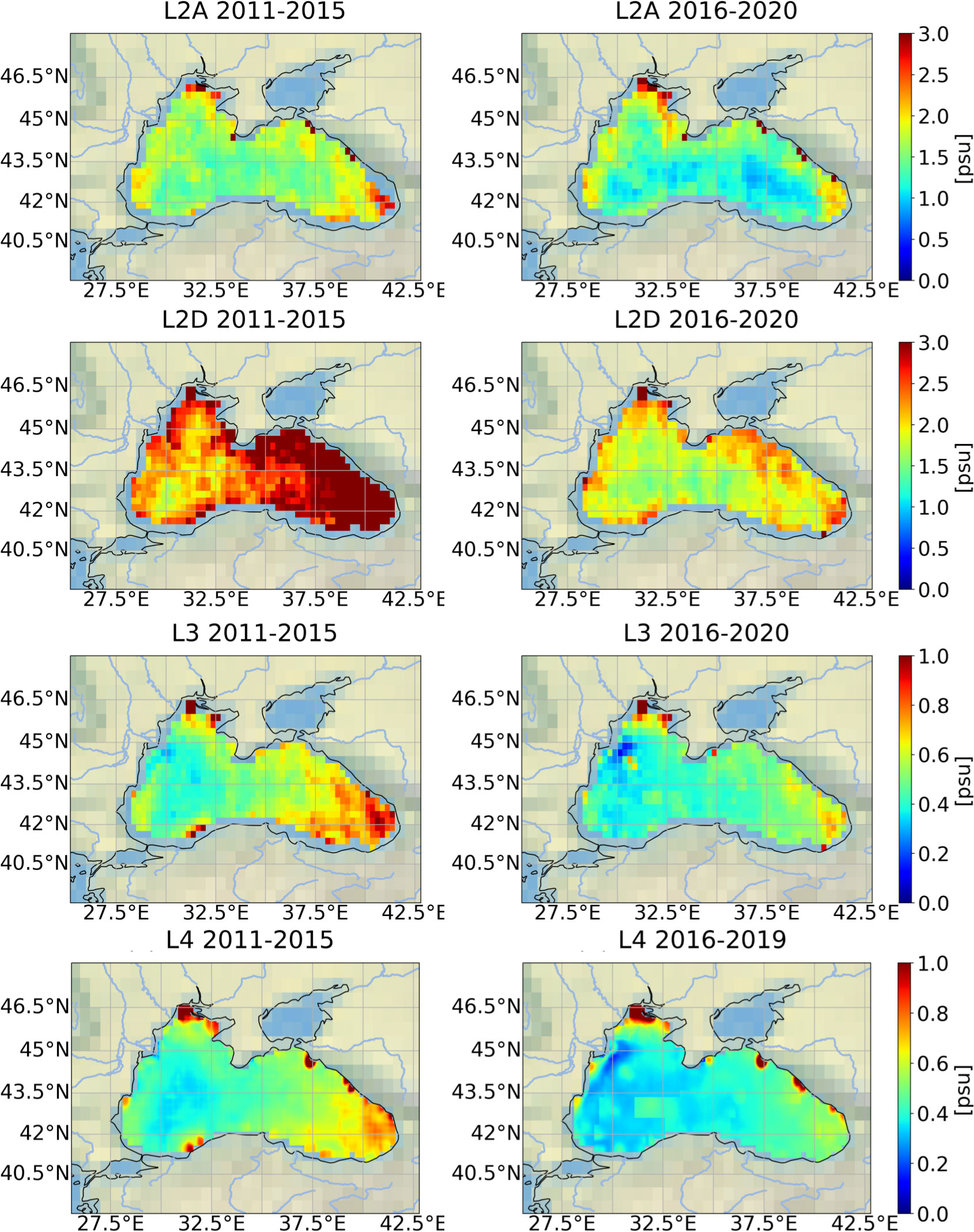
Figure 5 Spatial distribution of the uncertainty associated with the SSS product with respect to model simulations using the correlated triple collocation procedure for L2A (first row), L2B (second row), L3 (third row) and L4 (bottom) over 2011-2015 (left column) and 2016-2020 (right column).
The altimeter observing capability is defined by analyzing the SLA Power Spectral Density (PSD). It allows to define the minimum wavelength associated with the dynamical structures that the altimeter would statistically be able to observe with a signal-to-noise ratio (SNR) greater than 1 (i.e. the observable wavelength). The methodology applied is derived from Dufau et al. (2016) and consists in finding the wavelength for which the SNR is equal to 1, the signal being defined by the mesoscale spectral slope and the noise by a constant value fitted on the spectral plateau (or quite flat slope) visible at the shortest wavelengths. The determination of the spectral slope and noise is done by least square fitting a two-line sum model to the signal PSD. This analysis is done for both the 20Hz (i.e. upstream products for 5Hz product generation) and 1Hz altimeter raw (i.e. not low pass filtered) measurements provided by the Copernicus Marine Service for S3A and C2 missions. This analysis shows that the observing capability of the full rate measurement ranges between 25 (S3A) and 32 (C2) kms and is increased by a factor ~1.6 with respect to that of the 1Hz measurements that ranges between 40 (S3A) and 53 (C2) kms (Figure 6).
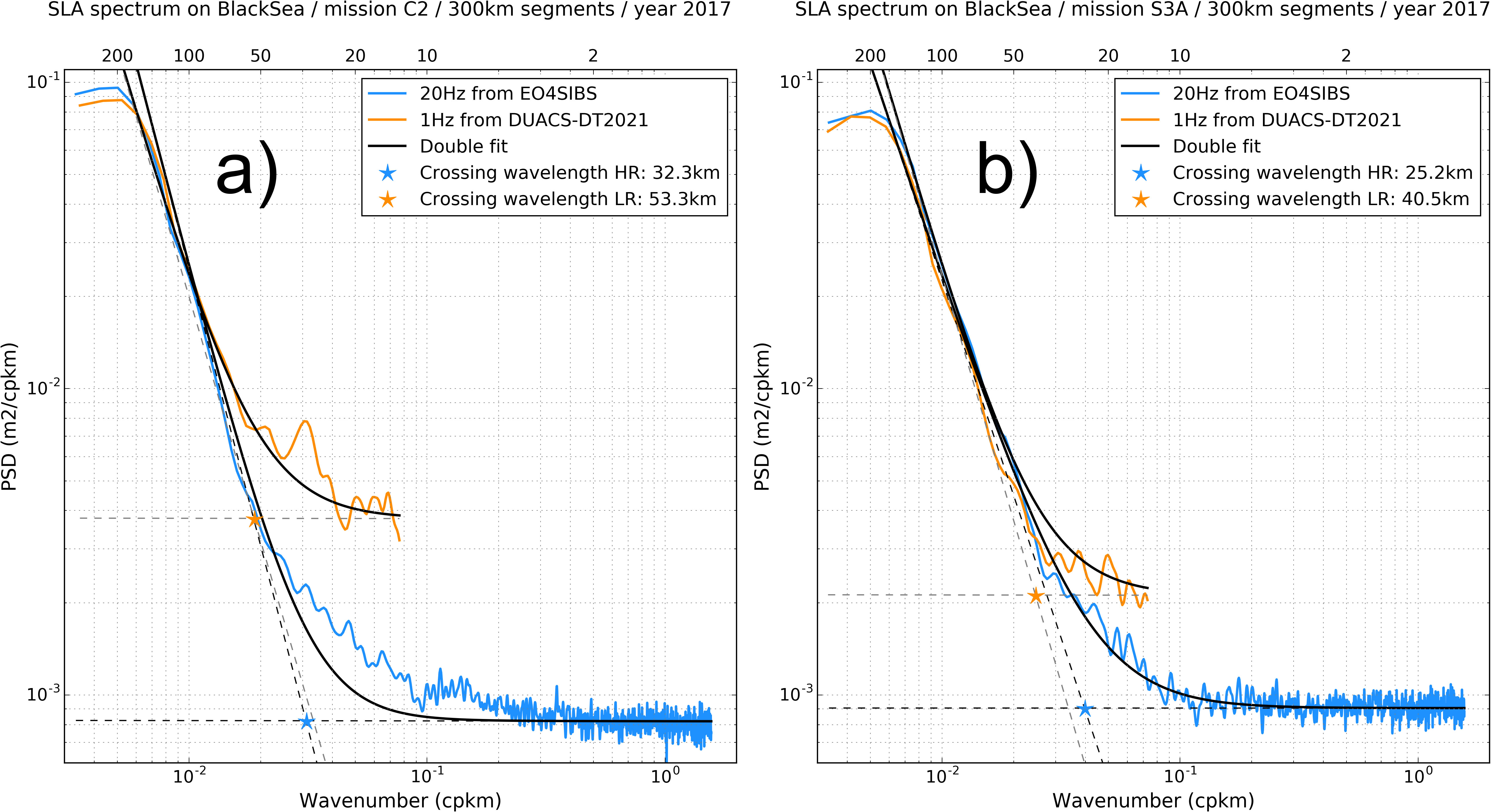
Figure 6 Mean SLA PSD over the Black Sea region, deduced from Cryosat-2 (A) and Sentinel-3A (B) measurements. The PSD obtained from 20Hz (resp. 1Hz) measurements is presented in blue (resp. orange). The spectral slope and noise level deduced from the PSD analysis are presented in dotted black lines, while theoretical spectrum, defined as the sum of the spectral slope and noise, are presented in thick black lines. The intersection between the spectral slope and noise level is symbolized by a blue (yellow) star for 20Hz (1Hz) measurements. It is representative of the SNR equal unity.
In Capet et al. (2022), the application of eddy detection and tracking algorithms to the EO4SIBS and Copernicus Marine Service gridded products confirms the enhanced capacity of the EO4SIBS products to describe mesoscale dynamics and eddy characterization: areas of formation dominant pathways, retrieved eddies properties and distinction between cyclones and anticyclones. In addition, the refined eddy mapping obtained with EO4SIBS Level-4 altimetry product allows a better characterization of subsurface anomalies of oxygen and temperature as evidenced by colocation of eddies with ARGO data.
The comparison of the seasonal cycle of SMOS SSS with that simulated by the Copernicus Marine Service physical model shows that SMOS SSS represents the main characteristics of the seasonal variability of the SSS spatial pattern in agreement with model simulations. The presence along the year of a freshwater plume (i.e. SSS <17 psu) formed by the discharges from mainly the Danube but also the Dniester and Dnieper over the northwestern shelf and advected along the coast by the Rim current is well represented (Figure 7). The extension of the plume from winter to summer along the basin is quite well visible even if SMOS SSS displays a band of low SSS values along the northeastern coast which is not clearly present in the model. Several spots of low SSS are present along this coast in association with the discharge from the Rioni and near the Kerch Strait connecting the Black Sea with the Azov Sea. Others seem to be due to local bathymetric features and/or river discharges. SMOS SSS underestimates the seasonal variability of the river plume dynamics over the shelf with a larger extension in winter and a lower extension in summer. We note however that an extension of river water over the shelf from winter to summer is visible in SMOS. SMOS is able to represent a salinification of the open sea from summer to winter in response to an enhanced mixing by turbulence and convection from October to March combined with an intensification of the Rim current that shallows the main pycnocline. However, the SMOS SSS above 19 psu in fall is too high compared to model results and Argo profiles (~6000 profiles) collected over the last 14 years that show surface salinity values between 17.5-18.7 psu (Stanev et al., 2019). This points to an overestimation of the SSS in the deep sea as already mentioned in Sect. 3. Yu (2010) shows that skin salinification can cause an increase of 0.05-0.15 in regions with high evaporation or/and low wind intensity. The summer-fall period is characterized by an excess of evaporation with respect to precipitation over most of the basin (Supplementary S5). This excess combined with an intensification of mixing explain the increase of SSS in fall but the SMOS values seem too high. This very large SMOS SSS is only present in 2017 and does not seem to be associated with any meteorological event. We have also exploited the capability of SMOS SSS product to track the freshwater plume to study the connection between SSS and Coloured Detrital Matter (CDM) with the final objective of retrieving a SMOS derived CDM product. One of the main advantages of this product is that, despite the coarse spatial resolution, it is an all-weather variable. This has a potential significant added value, especially in a basin that has a 40-50% of average cloud coverage (González-Haro et al., 2021).
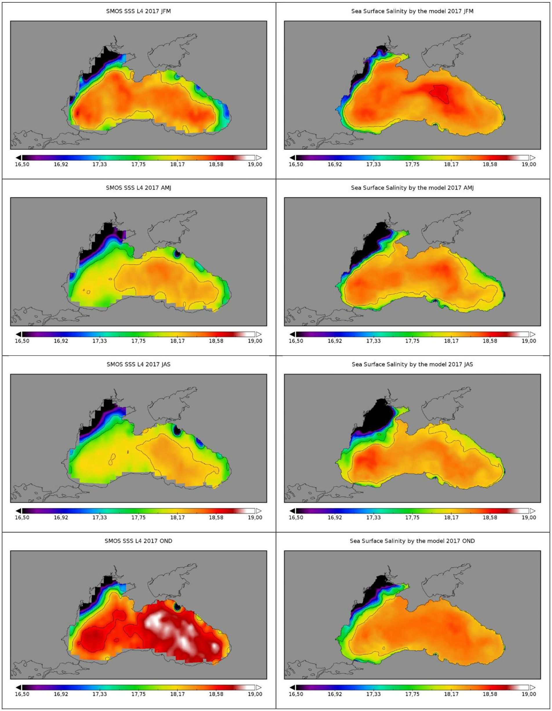
Figure 7 Seasonal evolution of the SSS from SMOS (left) and modelling (right) over 2017. First row: winter (January-February-March), second row: spring (April-May-June), third row: summer (July, August, September), Last row: fall (October, November, December).
Throughout the year, the highest concentrations of SPM are along the coast, more particularly, at the mouth of the main rivers (Danube, Dnieper, Rioni) and at the exit of the Kerch strait (Figure 8). In offshore and deep-sea regions, the SPM dynamics exhibits important variability with high values at basin scale in winter and during the massive surface development of coccolithophores as in early summer 2017. Lower values are observed in spring and fall. At the Danube’s mouths, the behaviour of the plume is consistent with the long-term dynamics (Constantin et al., 2017), with higher extension at the end of spring as for the SSS. Because SPM lumps all optically active near-surface suspended particles including both living (phytoplankton, zooplankton, bacteria), non-living organic (detritus) and mineral (sediments, coccolithophorid plates) materials, the understanding of its dynamics integrates physical and biogeochemical processes including flocculation/aggregation, deposition, resuspension, transport, bloom dynamics and river discharges. The dynamics of the biogenic SPM is predominantly governed by phytoplankton bloom and can be inferred from satellite Chl-a while that of mineral SPM is determined by the balance of river inputs and deposition-resuspension processes. Resuspension is expected to be the largest in winter due to enhanced wind waves while river inputs reach their peak in May. Model simulations by Stanev and Kandilarov (2012) found that the heavy SPM (i.e., coarse sediment) settles close to the river mouth and is trapped near the mouths of the rivers and in the southwestern coastal zone. On the other hand, fine sediment particles are transported away from river mouths via several deposition and resuspension events mainly driven by wind-waves. These events are responsible for the spatial extension over the shelf and coast of the riverine SPM and for their transfer to the deep sea. The grain size distribution of bottom sediment reflects this feature with the largest size (i.e., 20-63 µm) south of the Danube’s mouth where the shear stress is the highest (e.g. Wijsman et al., 1999), 6.3-63 µm along the slope area and <2 μm in the abyssal plain (Müller and Stoffers, 1974). In winter, high SPM values are observed at basin scale in response to the winter phytoplankton bloom and to the intense resuspension along the coast (e.g., western coast). The distribution is not uniform but exhibits mesoscale variability in the form of mushroom structures and elongated tongues associated with eddies and filaments (Figure 8). Then, in spring, the SPM sharply decreases in the central basin and over the north-western shelf as a result of the decrease of both bloom and wind intensity. The largest values of SPM are observed in June 2017 due to a massive coccolithophore algal bloom quite common during this period (Kubryakov et al., 2019; Kubryakova et al., 2021). This bloom was particularly intense in 2017 with satellite-derived SPM and Chl-a concentration (Figures 8, 9) two or even three times higher than during the same period in 2016. The algorithm simulates high Chl-a value in connection with the summer coccolithophores bloom (Figure 9). However, these high Chl-a values cannot be confirmed in-situ due to the lack of data. Previous finding indicates that Chl-a is generally low when coccolithophores blooms are detected, especially for winter blooms (Kubryakova et al., 2021). For early summer blooms, however, the relationship low Chl-a - high-coccolithophore abundances appears less significant. Indeed, during this period, favorable conditions for diatoms growth appear (Kubryakov et al., 2019). Diatoms and coccolithophores population could then co-exist during this transition phase, and this could partially explain the high values of Chl-a. In-situ data on coccolithophore abundances and Chl-a concentrations are needed at basin scale to validate this assumption. During this bloom, the composition of the SPM differs in the central basin where it is mainly made of Chl-a and on the north-western shelf where the mineral part dominates (Figure 10).
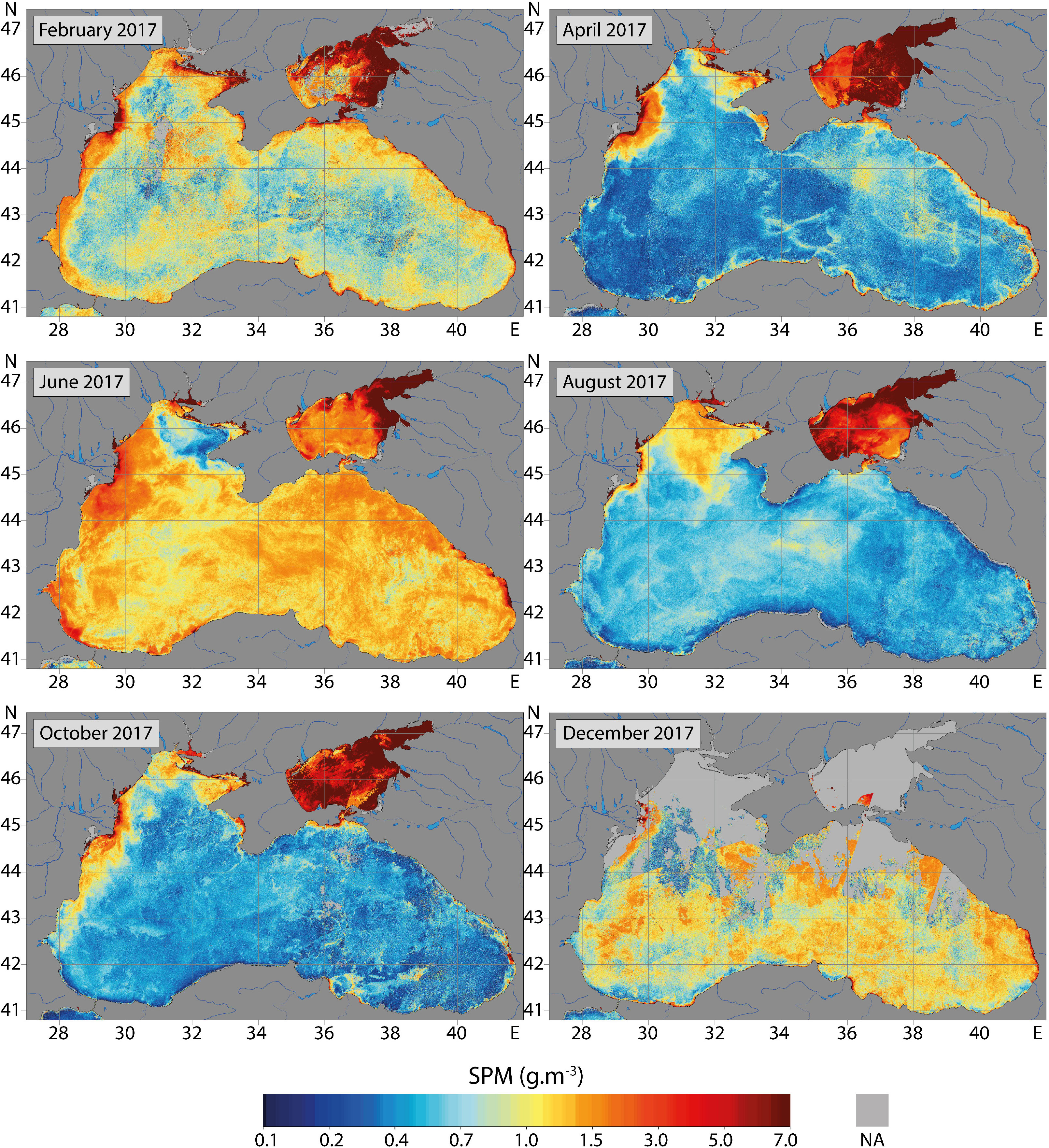
Figure 8 EO4SIBS SPM concentration maps (monthly composites) during selected months of 2017.
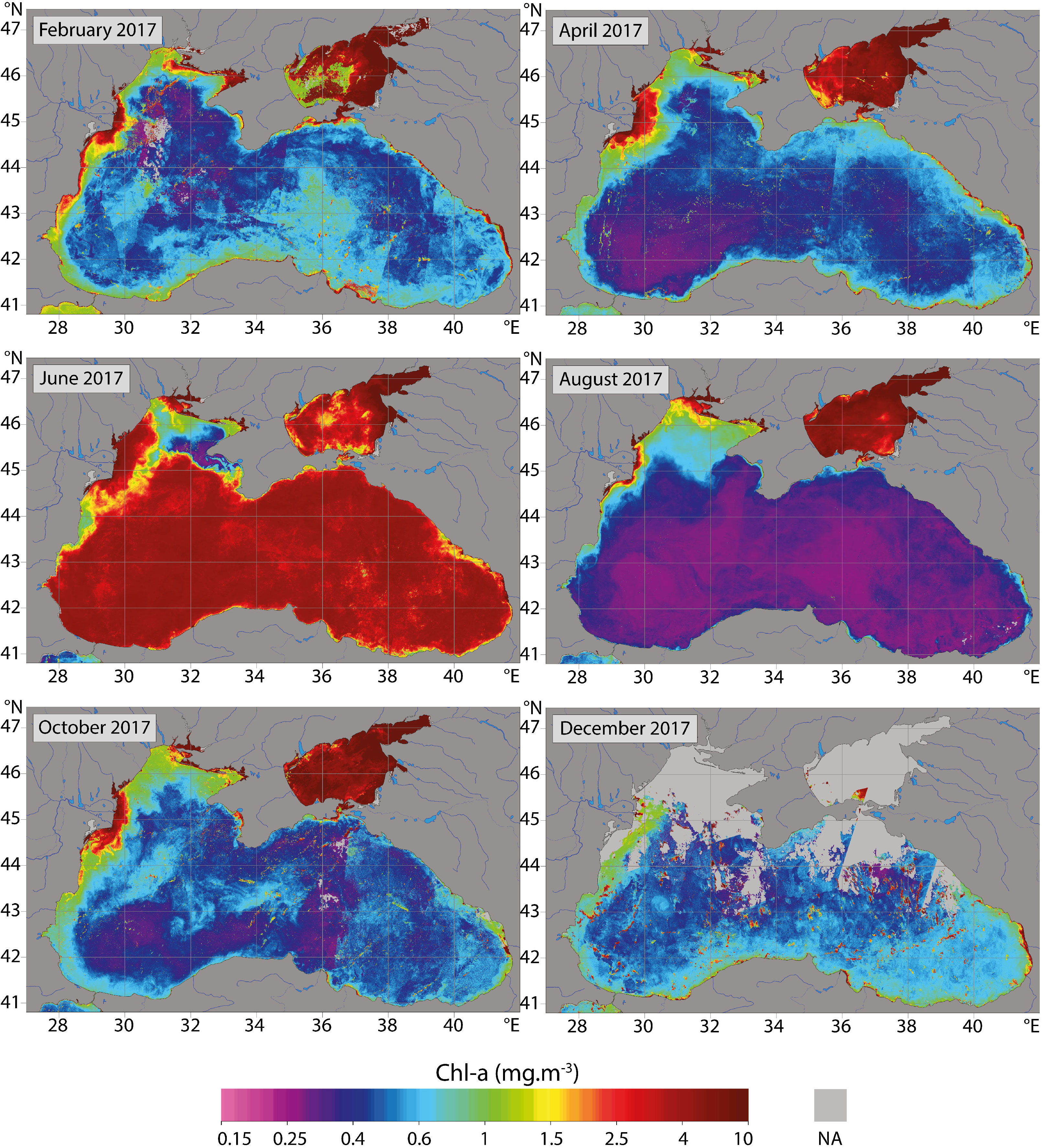
Figure 9 EO4SIBS Chl-a concentration maps (monthly composites) during selected months of 2017.
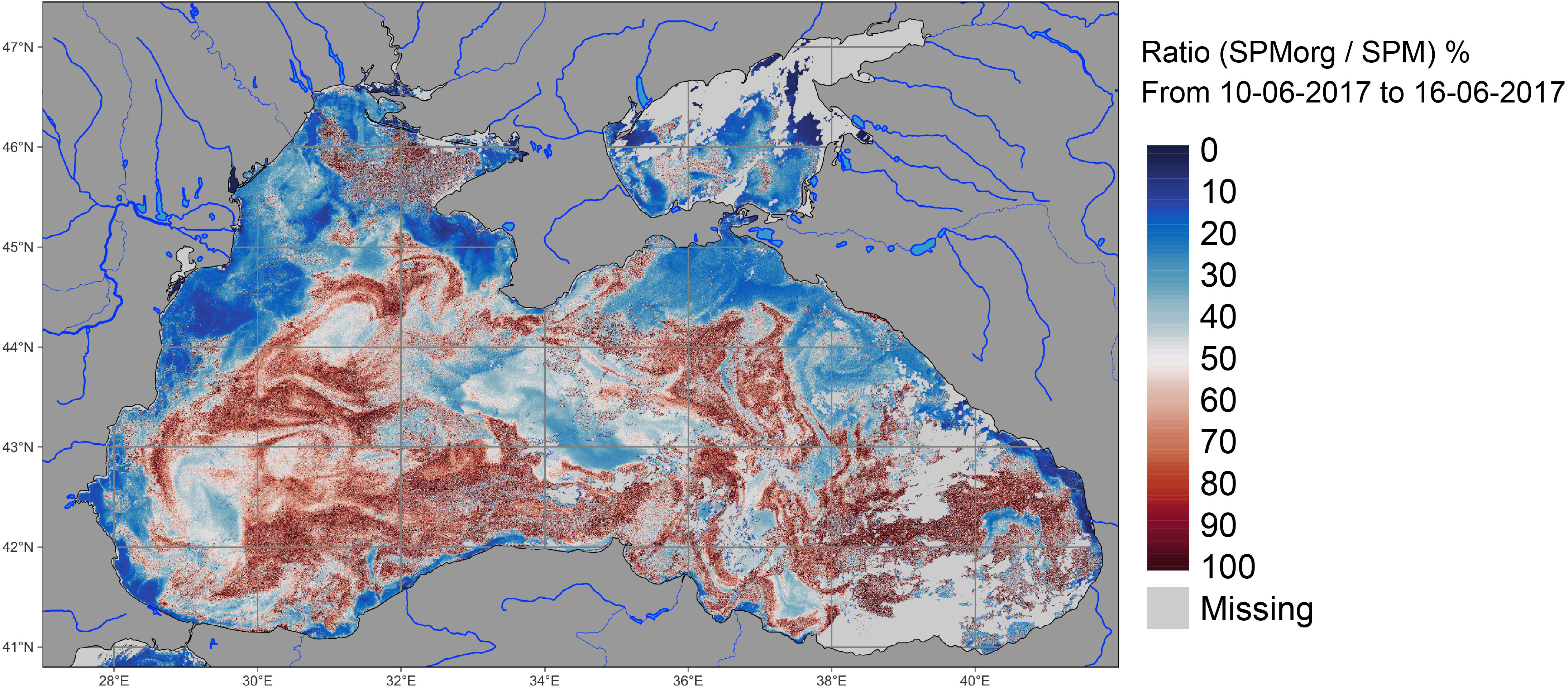
Figure 10 Map of the organic fraction (in %) of the SPM estimated during the coccolithophorid in June 2017 (weekly composite: 10-16 June 2017). This fraction has been computed using the approach described in Babin et al. (2003) (see their equations 1 and 2) using the estimated Chl-a as a proxy of the organic part.
In August, an anticyclonic gyre forms over the Black Sea northwestern shelf and transports northward riverine waters. The shelf is occupied by waters with high SPM and Chl-a values that penetrate towards the deep sea via filaments ejected at the shelf break (Figures 8, 9). It is during this period that bottom hypoxia may occur (e.g., Mee et al., 2005; Capet et al., 2013). In the deep sea, surface SPM and Chl-a are very low because the bloom occurs deeper and results in a deep chlorophyll maximum (e.g., Yunev et al., 2005; Ricour et al., 2021). In October, the extension of the bloom over the shelf is reduced due to the decrease of the river discharges and intensification of northern wind (Grégoire and Beckers, 2004; Grégoire et al., 2004).
The Black Sea is mostly occupied by case-1 water throughout the year, except during the coccolithophores bloom in June when a significant part of the sea becomes case-2, the exception of the northern part of the northwestern shelf (Figure 11). Case-2 waters are also found in August in the eastern part of the shelf. Case-3 waters are very localized, mainly at the mouth of the main rivers. Nevertheless, the distribution of water optical classes, as defined by the current approach, can be very dynamic in shorter periods of time. This comes to reinforce the necessity for class-specific algorithms definition and for the collection of adequate data for their validation.
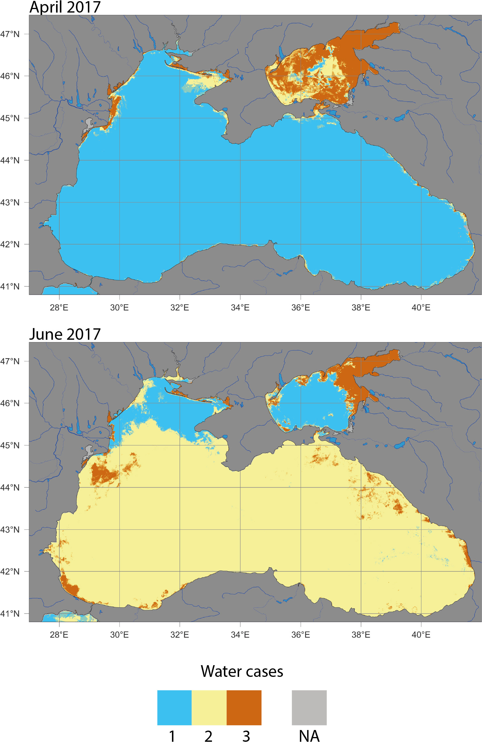
Figure 11 Water classification as Case 1, 2 or 3 (see the text for definitions) as monthly composites in April 2017 (top) and June 2017 (bottom).
The monitoring of the long-term evolution of the Mean Sea Level (MSL) for climate applications and the analysis of Ocean/Climate indicators (e.g., MSL trends) require a homogeneous and stable sea level record. Such a dataset is produced within the Copernicus Climate Service (C3S, Legeais and Meyssignac, 2021), which is considered as the reference product for MSL change detection. Trend in the MSL estimated from C3S is compared with that estimated with products from the Copernicus Marine Service and EO4SIBS (Figure 12). These last two products are more designed for mesoscale activities. The MSL trend is analyzed over the 10-year period common to the 3 products considered. Although a 10-year period is too short to give an accurate estimation of the MSL climate trend over the Black Sea, it allows to qualify the consistency of the different gridded products. The 10-year trend in the MSL obtained from these 3 gridded products show important differences with -0.11 ± 0.35 mm yr-1 for EO4SIBS, 0.07 ± 0.36 mm yr-1 for C3S and 1.17 ± 0.35 mm yr-1 for Copernicus Marine Service. The EO4SIBS MSL trend presents large (-0.178 mm yr-1) and very large (-1.28 mm yr-1) differences with trends obtained from C3S and Copernicus Marine Service regional reference products, respectively. Analyses suggest that a good part of these differences arises from the choice of the Mean Sea Surface (MSS) solution used in the processing. While C3S use the same gridded MSS reference for the processing of all the altimeter measurement used for this product, Copernicus Marine Service production rather considers Mean Profile (i.e., a MSS estimated along the track of the altimeter) for repetitive altimeter measurements (e.g., Jason-3 and Sentinel-3A over the period considered). The long wavelength pattern difference between these two MSS solutions can affect the stability of the MSL trend over regional areas such as the Black Sea as discussed in the C3S product quality document. Additionally, possible residual biases between SAR and LRM mode acquisition areas for C2 may also contribute to the MSL trend differences. Further analyses are however required to quantify this effect. Nevertheless, the better consistency of the MSL trend deduced from EO4SIBS products and reference two-satellite C3S products suggests an improvement compared to the CMEMS production. The use of higher frequency upstream data may have enhanced cross-calibration correction in the EO4SIBS multi-satellite processing.
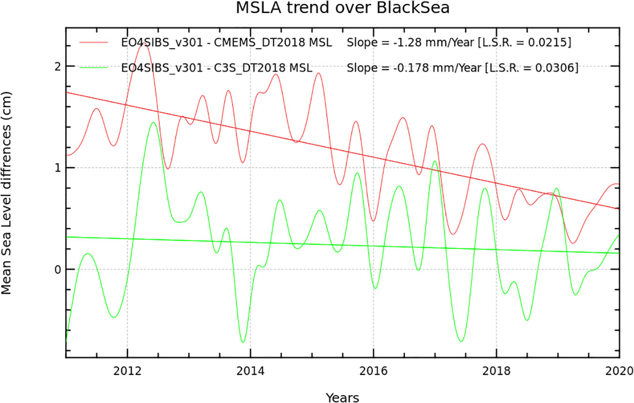
Figure 12 Difference of the Black Sea MSL trend estimation from EO4SIBS and Copernicus Marine Service (DT-2018 version) gridded products (red line) and from EO4SIBS and C3S (DT-2018 version) gridded products (green line).
These trends can be compared with that of 7.6 ± 0.3 mm yr-1 found over 1992-2005 by Kubryakov and Stanichnyi (2013) from along track Topex Poseidon and Jason 1 altimetry data and that of 27 ± 2.5 mm yr-1 obtained over 1993-1998 by Cazenave et al. (2002) using Topex Poseidon and ERS-1/2. However, this last estimate was obtained over 6 years and was ~15 times larger than the interdecadal trend derived from tide gauges (TG) which are of 1.8 ± 2.2 mm yr-1. The authors concluded that the larger altimetry derived sea level rise reflects more the multiyear fluctuations rather than the climatic signal that is possibly evidenced by TG measurements. The differences between these estimates of MSL rise can be explained by the use of different data, data treatments and period of computations. They also underlined the need for an improvement of coastal altimetry products validated by quality-controlled TG data over several decades.
In this paper, new algorithms and earth observation products related to OC, SSS and altimetry are described and their potentials analyzed for understanding the Black Sea dynamics. The products are developed at basin scale with specific treatments to improve their quality in the coastal areas.
The SMOS SSS Level-2, -3 and -4 products presented here are the first and cover 10 years from 2011-2020. This has required dedicated efforts for improving L-band data processing algorithms, especially focused on the mitigation of the RFI, but also to deal with the land-sea contamination and the challenge of the SSS retrieval in low temperature and low salinity water regimes. The comparison of SMOS SSS with in-situ and model data estimates the accuracy of the final EO4SIBS SMOS SSS products at 0.4-0.7 psu (Olmedo et al., 2022). This is a success taking into account that since the beginning of the SMOS mission it is evident that the environmental conditions of the Black Sea basin hamper the SSS retrieval. In comparison, the seasonal variability of the Black Sea SSS in the open sea in response to dilution, evaporation, mixing and river water intrusion amounts to a few tenths of psu (~0.1-0.5 psu).
For OC, Chl-a, SPM and TURB datasets are produced using regional calibrated algorithms. The application of a water classification algorithm highlights the heterogeneity of the Black Sea from optical point of view (e.g. mostly case-1 in open sea areas, with periods of class-2 and very localized case 3 waters). These regional products need to be further validated using datasets independent from the calibration ones, representative of the entire Black Sea and of all possible environmental conditions, including during coccolithophores blooms.
Here below we summarize the main novelties of this study and propose further developments for different Black Sea’s applications.
We deliver a 5Hz altimetry along-track product obtained by processing the full rate (20Hz) altimeter measurements from C2 and S3A. This 5Hz product is combined with existing 1Hz product and interpolated to produce gridded datasets for the SLA, mean dynamic topography, geostrophic currents. We show that these EO4SIBS altimetry products offer, compared to a 1Hz one, a better definition of the main Black Sea current, a more accurate reconstructions of eddies structure in coastal areas and improve the observable wavelength by a factor 1.6. It also allows a better characterization of the mesoscale circulation with, in particular, an improved identification and characterization of eddies.
For SSS, we show that the SMOS product tracks the basic characteristics of the Danube’s plume dynamics with an increased extension at the plume at the end of spring when the discharge is maximum. However, SMOS SSS underestimates the variability of the plume dynamics. An increased resolution of Level-2 products for coastal applications can be achieved by combining the SMOS retrieved brightness temperature with SST from S2 and S3, using non-linear fusion schemes. A consideration of the day-night temperature cycle is also expected to improve the resolution of the Level-2 product.
For OC, the combination of different datasets from S2 and S3 using appropriate fusions techniques is promising for the delivery of very high-resolution products for coastal applications. For instance, fusion between S2-MSI and S3-OLCI data can bring benefits in areas where a detailed inspection of the spatial patterns combined with improved spectral information is needed (Alvera-Azcárate et al., 2021). The comparison of cloud-free S2-MSI and S3-OLCI satellite images obtained over three coastal optically complex areas (i.e., ROFIs regions, one of them being close to a port) shows consistency between S2-MSI and S3-OLC for the green and red bands but this consistency tends to decrease for other spectral regions requiring specific treatments.
The MSL trend estimation and associated error budget in the Black Sea region may still be improved. Estimates of MSL rise range from -0.11 to 27 mm yr-1. These uncertainties arise from the use of different data types, treatments and periods of estimation. For the future, an improvement of the quality of Level-3 and Level-4 altimetry products is proposed along four main directions in order to better constrain the MSL rise estimation and, in particular, to improve the quality of the product in the coastal ocean. 1) Extend the full rate altimeter processing to additional altimeter nadir measurement, and continue to improve the processing. 2) Progress in the understanding of the altimeter capabilities and limitations, especially with new altimeter technologies. 3) A better characterization for the Black Sea of the pertinence and quality of geophysical and environmental corrections classically used in altimeter processing. 4) Improve mapping methodologies. The merging with in-situ measurements (e.g. drifters, TG) may also contribute to improve the signal reconstruction near the coast. It is critical to maintain a TG network able to monitor the long-term variability of the sea level with a consistent processing.
The assessment of climate impact on SSS is still not clear. Alterations of the thermohaline Black Sea state has been recently evidenced from the analysis of Argo data (Stanev et al., 2019). These alterations are associated to changes in the vertical diapycnal mixing at the depth of the main pycnocline due to CIL erosion that cause an increase of the salinity in the surface layer. Miladinova et al. (2017) modeled a small increase of 0.02 of the SSS. The small amplitude of the signal to capture puts significant constraints on the SMOS SSS. The analysis of the accuracy of the SMOS SSS in comparison with ARGOs over the last decade does not show drift in the quality of the product but rather incoherent noise which is encouraging (Supplementary S6).
Satellite products are more and more used for assessing climate change and the near-real time monitoring of ocean health (e.g., Morrow et al., 2018; Groom et al., 2019; Vinogradova et al., 2019). Yet, their use in understanding marine deoxygenation is still limited although coastal hypoxia is a worldwide phenomenon (e.g. Breitburg et al., 2018; Fennel and Testa, 2019; Grégoire et al., 2019; Pitcher et al., 2021).
The combination of OC, SSS and altimetry products can be used to identify potential critical regions for the generation of hypoxia by monitoring the plume dynamics, regions of enhanced productivity and stratification duration. The combination of these satellite products with in-situ real time monitoring (e.g., mooring, profilers) and model forecasting will constitute an ideal system for alerting on hypoxia.
In the open sea, the formation of the CIL constitutes one of the main processes of ventilation of the subsurface layer. Because the amplitude of the seasonal thermal buoyancy flux exceeds that of the haline buoyancy flux by an order of magnitude, density variability in the upper 50m is mainly governed by temperature variability. Due to that and to the lack of SSS at basin scale, the role of salinity in the CIL dynamics has been less investigated than that of temperature with some noticeable exceptions (e.g., Stanev et al., 2019). The potential of SST and SSS products to map areas that meet the two necessary conditions for having formation of cold intermediate waters (i.e., SST < 8°C and density larger than 14.5, Stanev et al., 2003) can be investigated thanks to SMOS SSS.
Capet et al. (2022) evidence that the EO4SIBS Level-4 altimetry dataset better characterize subsurface anomalies of oxygen and salinity within cyclonic and anticyclonic eddies. The imprint of mesoscale structure on the oxygen distribution inside eddies is not limited to a vertical displacement. Other changes potentially induced by within-eddy biogeochemical processes are suggested. This finding is in agreement with that of Karstensen et al. (2015) who show that eddies are local sites of enhanced production and degradation of organic matter.
The combination of SST, SSS and altimetry satellite products with increased resolution and quality in connection with models and in-situ platforms offer information to progress in the understanding of the role of mesoscale and SSS in the formation of the CIL and evolution of Black Sea’s thermohaline state.
The development of OC, altimetry and SSS products for the period 2010-2020 has suffered from the lack of fit for purpose in-situ data for the calibration and validation of the algorithms. Table 2 summarizes the requirements for in-situ observations and gaps that are identified for developing the products listed in Table 1. In general, except for Argo, most in-situ data available in public databases (e.g., EMODnet, CMEMS, WOD) are collected in the frame of local campaigns, are very coastal and mostly cover the western basin (e.g., Palazov et al., 2019). The quality is sometimes not optimal and would benefit from best practices documentation and inter-calibration exercises across regions and basins.
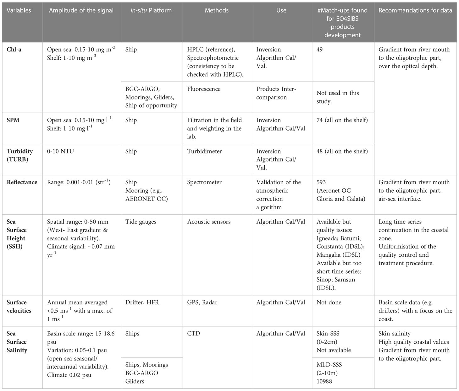
Table 2 Requirements for an observing system to support the development of EO products related to OC, SSS, altimetry.
For OC, the available in-situ data over the S3 and S2 periods are very limited and do not allow a validation of the products over the full spectrum of contrasted optical conditions present in the Black Sea. For Chl-a, high quality data, determined ideally by High Performance Liquid Chromatography (HPLC), is usually recommended. Yet, such data are very rarely available. For turbidity, SPM and CDOM, very few (no) data are available in the open sea. For SSS, most of the in-situ data used are collected from 1-10m (the shallowest). In the past, the Black Sea MSL has been quite well monitored by TG with data series longer than 100 years along the north-eastern coast (Figure 13, Table S2.2 and Supplementary S2). However, presently, the number of active TG significantly decreases and is mainly limited to the southern coast where two radars have been recently installed. In addition, the disparity in temporal series (e.g. gaps in time series), sampling and anomalies detected on the data series (e.g., no clear quality flagging) challenge to obtain significant results.
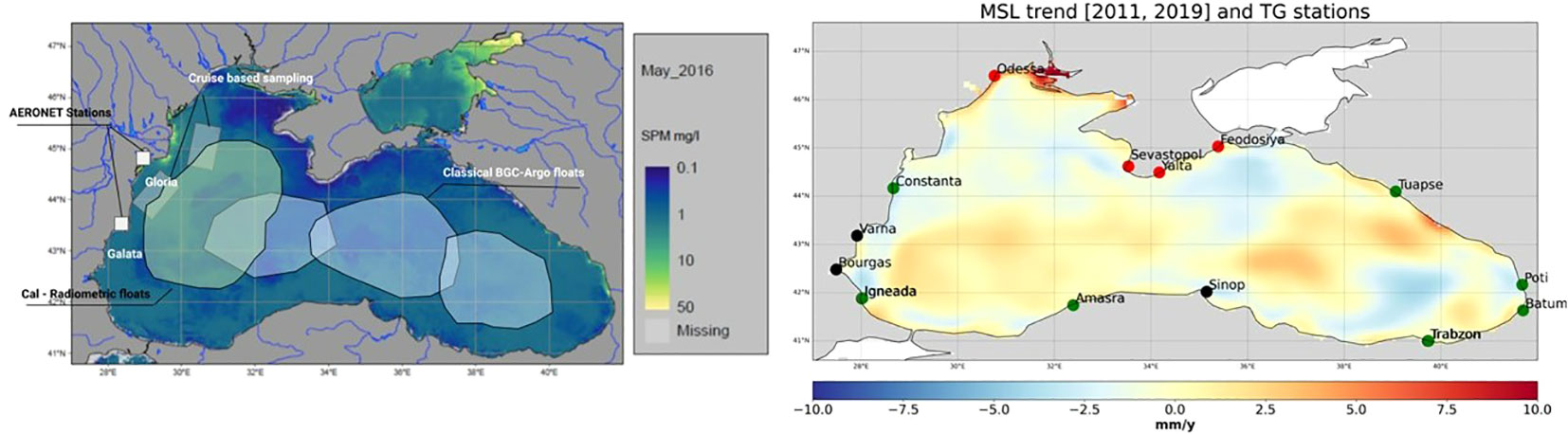
Figure 13 Mapping of the approximate positions of the different components of a Black Sea in-situ observing system to support (left) the development of OC products with SPMs superimposed, (right) the validation of altimetry products and estimation of the MSL. For OC, position of current Aeronet OC and suggestion for ship cruises and areas of deployment of BGC Argo are shown. For altimetry, position and names of tide gauge (TG) are indicated with different colour corresponding to the length of the dataset and its extension over recent years. In green, TG datasets are available to validate the MSL trend derived from altimetry (selection criteria: duration of the dataset > 10 years with datasets delivered recently i.e. >2015). In red, Russian TG datasets extend at least over 1992-2005. In black, TG datasets that cannot be used for the validation of the MSL trend (i.e., less than 10 years in common with the altimetry era).
Then, our recommendations for the evolution of the in-situ Black Sea observing system to support the development of high-quality satellite products on OC, SSS and altimetry are:
1. To reinforce and sustain the existing AERONET-OC network, which could inform and assess the quality of atmospheric correction algorithms. So far, two stations are present, and both are located along the western coast.
2. To deploy and permanently maintain 3 BGC-Argo floats, equipped with CDOM, Chl-a, backscatter and irradiance sensors in the eastern, central and western parts of the open sea (Figure 13).
3. To deploy at least 1 BGC-Argo float specifically equipped with hyperspectral radiance and irradiance instruments to provide high quality spectrally resolved radiometric data (e.g., spectral reflectance and irradiance, backscattering coefficients) (i.e., PROVAL, Leymarie et al., 2018; Xing et al., 2020).
4. To organize regular (i.e. two times/year) ship expeditions to collect along a coastal-offshore transect and ROFI regions an exhaustive high quality in-situ data set (i.e., radiometric, biogeochemical, skin salinity) for algorithms calibration and validation.
5. To continue the monitoring of sea level at historical stations where long data series are already available (e.g., Constantza, Batumi, Poti, Tuapse, Trabzon) and improve the processing, quality check, flagging and analysis of existing TG data at different scales (high frequency, monthly, yearly, …). Assure a monitoring covering the different coastal regions (currently, TG data are only available at three stations along the southern coast) (Figure 13).
6. To deploy drifters and high frequency radar radial measurement to validate the altimeter products.
7. To coordinate Observing System Experiments (OSEs) and Observing System Simulation Experiments (OSSEs) across regions to assess the benefit of satellite products on the quality of forecasting and reanalysis systems and to provide recommendations for missions development and observing network deployment.
The datasets generated for this study can be found on the web interface (http://www.eo4sibs.uliege.be/) and on Zenodo under data doi: 10.5281/zenodo.6397223 with a full documentation that include Products User Manuals (PUM) and Algorithm Theoretical Basis Document (ATBD). All these products are distributed in netCDF files Grégoire et al. (2022). SMOS SSS and CDM products are also available at https://bec.icm.csic.es/bec-ftp-service/.
MGr writes the manuscript with contributions from all the authors. All the authors discussed and reviewed the manuscript. MG is the project coordinator and M-HR is the ESA project officer. Altimetry products have been delivered by Collecte Localisation Satellites (CLS), Ocean Colour products by Terrasigna and Sorbonne University, Sea Surface Salinity products by Barcelona Expert Center (BEC) and Institute of Marine Sciences (ICM), CSIC. All authors contributed to the article and approved the submitted version.
This work has been carried out as part of the European Space Agency contract Earth Observation data For Science and Innovations in the Black Sea (EO4SIBS, ESA contract n° 4000127237/19/I-EF). MG received fundings from the Copernicus Marine Service (CMEMS), the European Union’s Horizon 2020 BRIDGE-BS project under grant agreement No. 101000240 and by the Project CE2COAST funded by ANR(FR), BELSPO (BE), FCT (PT), IZM (LV), MI (IE), MIUR (IT), Rannis (IS), and RCN (NO) through the 2019 “Joint Transnational Call on Next Generation Climate Science in Europe for Oceans” initiated by JPI Climate and JPI Oceans. The research on SMOS SSS has been also supported in part by the Spanish R&D project INTERACT (PID2020-114623RB-C31), which is funded by MCIN/AEI/10.13039/501100011033, funding from the Spanish government through the “Severo Ochoa Centre of Excellence” accreditation (CEX2019-000928-S) and the CSIC Thematic Interdisciplinary Platform Teledetect.
The authors thank the two reviewers who provided very helpful comments. .
The authors declare that the research was conducted in the absence of any commercial or financial relationships that could be construed as a potential conflict of interest.
All claims expressed in this article are solely those of the authors and do not necessarily represent those of their affiliated organizations, or those of the publisher, the editors and the reviewers. Any product that may be evaluated in this article, or claim that may be made by its manufacturer, is not guaranteed or endorsed by the publisher.
The Supplementary Material for this article can be found online at: https://www.frontiersin.org/articles/10.3389/fmars.2022.998970/full#supplementary-material
Akpinar A., Fach B. A., Oguz T. (2017). Observing the subsurface thermal signature of the black Sea cold intermediate layer with argo profiling floats. Deep Sea Res. Part I: Oceanographic Res. Papers 124, 140–152. doi: 10.1016/j.dsr.2017.04.002
Alvera-Azcárate A., Barth A., Rixen M., Beckers J.-M. (2005). Reconstruction of incomplete oceanographic data sets using empirical orthogonal functions: application to the Adriatic Sea surface temperature. Ocean Model. 9, 325–346. doi: 10.1016/j.ocemod.2004.08.001
Alvera-Azcárate A., Sirjacobs D., Barth A., Beckers J.-M. (2012). Outlier detection in satellite data using spatial coherence. Remote Sens. Environ. 119, 84–91. doi: 10.1016/j.rse.2011.12.009
Alvera-Azcárate A., Barth A., Troupin C., Beckers J.-M., Van der Zande D. (2021). Creation of high resolution suspended particulate matter data in the North Sea from Sentinel-2 and Sentinel-3 data. In 2021 IGARSS: IEEE International Geoscience & Remote Sensing Symposium. Proceedings. Brussels (Belgium). doi: 10.1109/IGARSS47720.2021.9554197
Antoine D., Morel A. (1999). A multiple scattering algorithm for atmospheric correction of remotely sensed ocean colour (MERIS instrument): principle and implementation for atmospheres carrying various aerosols including absorbing ones. Int. J. Remote Sens. 20, 1875–1916. doi: 10.1080/014311699212533
Babin M., Morel A., Fournier-Sicre V., Fell F., Stramski D. (2003). Light scattering properties of marine particles in coastal and open ocean waters as related to the particle mass concentration. Limnol. Oceanogr. 48 (2), 843–859. doi: 10.4319/lo.2003.48.2.0843
Beckers J.-M., Barth A., Alvera-Azcárate A. (2006). DINEOF reconstruction of clouded images including error maps – application to the Sea-surface temperature around Corsican island. Ocean Sci. 2, 183–199. doi: 10.5194/os-2-183-2006
Beckers J.-M., Rixen M. (2003). EOF calculations and data filling from incomplete oceanographic datasets. J. Atmos. Ocean. Tech. 20, 1839–1856. doi: 10.1175/1520-0426(2003)020<1839:ECADFF>2.0.CO;2
Bouzaiene M., Menna M., Elhmaidi D., Dilmahamod A. F., Poulain P.-M. (2021). Spreading of Lagrangian particles in the black Sea: A comparison between drifters and a high-resolution ocean model. Remote Sens 13 (13), 2603. doi: 10.3390/rs13132603
Breitburg D., Levin L. A., Oschlies A., Grégoire M., Chavez F. P., Conley D. J., et al. (2018). Declining oxygen in the global ocean and coastal waters. Science 359:1–11. doi: 10.1126/science.aam7240
Buesseler K., Livingston H., Ivanov L., Romanov A. (1991). Stability of the oxic–anoxic interface in the black Sea. Deep Sea Res. 41, 283–296. doi: 10.1016/0967-0637(94)90004-3
Capet A., Beckers J.-M., Grégoire M. (2013). Drivers, mechanisms and long-term variability of seasonal hypoxia on the black Sea northwestern shelf – is there any recovery after eutrophication? Biogeosciences 10, 3943–3962. doi: 10.5194/bg-10-3943-2013
Capet A., Troupin C., Cartensen J., Grégoire M., Beckers J.-M. (2014). Untangling spatial and temporal trends in the variability of the Black Sea Cold Intermediate Layer and mixed Layer Depth using the DIVA detrending procedure. Ocean Dynamics 64 (3), 315–324. doi: 10.1007/s10236-013-0683-4
Capet A., Stanev E. V., Beckers J.-M., Murray J. W., Grégoire M. (2016). Decline of the black Sea oxygen inventory. Biogeosciences 13, 1287–1297. doi: 10.5194/bg-13-1287-2016
Capet A., Taburet G., Mason E., Pujol M. I., Grégoire M., Rio M. H. (2022). Using argo floats to characterize altimetry products: a study of eddy-induced subsurface oxygen anomalies in the black Sea. Front. Mar. Sci 9, 875653. doi: 10.3389/fmars.2022.875653
Capet A., Vandenbulcke L., Grégoire M. (2020). A new intermittent regime of convective ventilation threatens the black Sea oxygenation status. Biogeosciences 17, 6507–6525. doi: 10.5194/bg-17-6507-2020
Cazenave A., Bonnefond P., Mercier F., Dominh K., Toumazou V. (2002). Sea Level variations in the Mediterranean Sea and black Sea from satellite altimetry and tide gauges. Global Planet. Change 34, 59–86. doi: 10.1016/S0921-8181(02)00106-6
Ciliberti S. A., Grégoire M., Staneva J., Palazov A., Coppini G., Lecci R., et al. (2021). Monitoring and forecasting the ocean state and biogeochemical processes in the black Sea: Recent developments in the Copernicus marine service. J. Mar. Sci. Eng. 9, 1146. doi: 10.3390/jmse9101146
Constantin S., Constantinescu Ș., Doxaran D. (2017). Long-term analysis of turbidity patterns in Danube delta coastal area based on MODIS satellite data. J. Mar. Syst. 170, 10–21. doi: 10.1016/j.jmarsys.2017.01.016
Constantin S., Doxaran D., Constantinescu Ș. (2016). Estimation of water turbidity and analysis of its spatio-temporal variability in the Danube river plume (Black Sea) using MODIS satellite data. Cont. Shelf Res. 112, 14–30. doi: 10.1016/j.csr.2015.11.009
Davis R. E. (1998). Preliminary results from directly measuring mid-depth circulation in the tropical and south pacific. J. Geophys. Res.-Oceans 103, 24619–24639. doi: 10.1029/98JC01913
Degens E. T., Ross D. A. (1972). Chronology of the black Sea over the last 25,000 years. Chem. Geol. 10, 1–16. doi: 10.1016/0009-2541(72)90073-3
Doerffer R., Schiller H. (2007). The MERIS case 2 water algorithm. Int. J. Remote Sens. 28, 517–535. doi: 10.1080/01431160600821127
Dogliotti A. I., Ruddick K., Nechad B., Doxaran D., Knaeps E. (2015). A single algorithm to retrieve turbidity from remotely-sensed data in all coastal and estuarine waters. Remote Sens. Environ. 156, 157–168. doi: 10.1016/j.rse.2014.09.020
Dufau C., Orsztynowicz M., Dibarboure G., Morrow R., Le Traon P.-Y. (2016). Mesoscale resolution capability of altimetry: Present and future. J. Geophys. Res.-Oceans 121, 4910–4927. doi: 10.1002/2015JC010904
Dussurget R., Birol F., Morrow R., Mey P. D. (2011). Fine resolution altimetry data for a regional application in the bay of Biscay. Mar. Geod. 34, 447–476. doi: 10.1080/01490419.2011.584835
Escudier R., Bouffard J., Pascual A., Poulain P.-M., Pujol M.-I. (2013). Improvement of coastal and mesoscale observation from space: Application to the northwestern Mediterranean Sea. Geophys. Res. Lett. 40, 2148–2153. doi: 10.1002/grl.503242
EUMETSAT (2021) Sentinel-3 OLCI L2 report for baseline collection OL_L2M_003. doc. no. EUM/RSP/REP/21/1211386. Available at: https://www.eumetsat.int/media/47794.
Fennel K., Testa J. M. (2019). Biogeochemical controls on coastal hypoxia. Annu. Rev. Mar. Sci. 11, 105–130. doi: 10.1146/annurev-marine-010318-095138
González-Gambau V., Olmedo E., Turiel A., González-Haro C., García- Espriu A., Martínez J., et al. (2022). First SMOS Sea surface salinity dedicated products over the Baltic Sea. Earth Syst. Sci. Data Discussions 14 (5), 2343–2368. doi: 10.5194/essd-2021-461
González-Gambau V., Olmedo E., Turiel A., Martínez J., Ballabrera-Poy J., Portabella M., et al. (2016). Enhancing SMOS brightness temperatures over the ocean using the nodal sampling image reconstruction technique. Remote Sens. Environ. 180, 205–220. doi: 10.1016/j.rse.2015.12.032
González-Gambau V., Turiel A., González-Haro C., Martínez J., Olmedo E., Oliva R., et al. (2020). Triple collocation analysis for two error-correlated datasets: Application to l-band brightness temperatures over land. Remote Sens-Basel 12, 3381. doi: 10.3390/rs12203381
González-Haro C., Olmedo E., González-Gambau V., García-Espriu A., Turiel A. (2021). “EO4SIBS experimental SMOS Colored Detrital Matter (CDM) L4 (V.1.0) [Dataset]”; DIGITAL.CSIC. doi: 10.20350/digitalCSIC/14000. Available at: http://hdl.handle.net/10261/252461.
Goyens C., Jamet C., Schroeder T. (2013). Evaluation of four atmospheric correction algorithms for MODIS-aqua images over contrasted coastal waters. Remote Sens. Environ. 131, 63–75. doi: 10.1016/j.rse.2012.12.006
Grégoire M., Alvera-Azcarate A., Buga L., Capet A., Constantin S., D’ortenzio F., et al. (2022) EO4SIBS products, ESA, dataset (Zenodo). doi: 10.5281/zenodo.6397224
Grégoire M., Beckers J.-M. (2004). Modeling the nitrogen fluxes in the black Sea using a 3D coupled hydrodynamical-biogeochemical model: transport versus biogeochemical processes, exchanges across the shelf break and comparison of the shelf and deep sea ecodynamics. Biogeosciences 1, 33–61. doi: 10.5194/bg-1-33-2004
Grégoire M., Gilbert D., Oschlies A., Rose K. (2019). What is ocean deoxygenation? In Laffoley D., Baxter J. M. (eds.) (2019) Ocean deoxygenation: Everyone’s problem - Causes, impacts, consequences and solutions, (Gland, Switzerland: IUCN) xxii+562pp. doi: 10.2305/IUCN.CH.2019.13.en
Grégoire M., Lacroix G. (2001). Study of the oxygen budget of the black Sea waters using a 3D coupled hydrodynamical-biogeochemical model. J. Mar. Syst. 31, 175–202. doi: 10.1016/S0924-7963(01)00052-5
Grégoire M., Soetaert K., Nezlin N. P., Kostianoy A. G. (2004). Modeling the nitrogen cycling and plankton productivity in the black Sea using a three-dimensional interdisciplinary model. J. Geophys. Res.-Oceans 109 (C5), C05007. doi: 10.1029/2001JC001014
Groom S., Sathyendranath S., Ban Y., Bernard S., Brewin R., Brotas V., et al. (2019). Satellite ocean colour: current status and future perspective. Front. Mar. Sci. 6, 485. doi: 10.3389/fmars.2019.00485
Kajiyama T., D’Alimonte D., Zibordi G. (2018). Algorithms merging for the determination of chlorophyll-a concentration in the black sea. IEEE Geosci. Remote S. 16, 677–681. doi: 10.1109/LGRS.2018.2883539
Karstensen J., Fiedler B., Schütte F., Brandt P., Körtzinger A., Fischer G., et al. (2015). Open ocean dead zones in the tropical north Atlantic ocean. Biogeosciences 12, 2597–2605. doi: 10.5194/bg-12-2597-2015
Konovalov S., Murray J. (2001). Variations in the chemistry of the black Sea on a time scale of decades, (1960 – 1995). J. Mar. Syst., 31 (1-3), 217–243. doi: 10.1016/S0924-7963(01)00054-9
Kopelevich O., Sheberstov S., Yunev O., Basturk O., Finenko Z., Nikonov S., et al. (2002). Surface chlorophyll in the black Sea over 1978–1986 derived from satellite and in situ data. J. Mar. Syst. 36, 145–160. doi: 10.1016/S0924-7963(02)00184-7
Kubryakova E., Kubryakov A., Mikaelyan A. (2021). Winter coccolithophore blooms in the black Sea: Interannual variability and driving factors. J. Mar. Syst., 213, 103461. doi: 10.1016/j.jmarsys.2020.103461
Kubryakova E., Kubryakov A., Mikaelyan A (2019). Summer and winter coccolithophore blooms in the black Sea and their impact on production of dissolved organic matter from bio-argo data. J. Mar. Syst. 199, 103220. doi: 10.1016/j.jmarsys.2019.103220
Kubryakov A. A., Stanichny S. V. (2015). Seasonal and interannual variability of the black Sea eddies and its dependence on characteristics of the large-scale circulation. Deep Sea Res. Part I: Oceanographic Res. Papers 97, 80–91. doi: 10.1016/j.dsr.2014.12.002
Kubryakov A., Stanichnyi S. (2013). The black Sea level trends from tide gages and satellite altimetry. Russian Meteorology Hydrology 38, 329–333. doi: 10.3103/S1068373913050051
Kurkin A., Kurkina O., Rybin A., Talipova T. (2020). Comparative analysis of the first baroclinic rossby radius in the Baltic, black, Okhotsk, and Mediterranean seas. Russian J. Earth Sci. 20, ES4008. doi: 10.2205/2020ES000737
Legeais J.-F., Meyssignac B. (2021). C3S, Sea level product quality assessment report. D2.SL.2-v2.0_PQAR_of_v2DT2021_SeaLevel_products_v1.0 (Copernicus Climate Change Service & ECMWF). Available at: https://datastore.copernicus-climate.eu/documents/satellite-sea-level/vDT2021/D2.SL.2-v2.0_PQAR_of_v2DT2021_SeaLevel_products_v1.0_APPROVED_Ver1.pdf.
Le Traon P., Nadal F., Ducet N. (1998). An improved mapping method of multisatellite altimeter data. J. Atmos. Ocean. Tech. 15, 522–534. doi: 10.1175/1520-0426(1998)015<0522:AIMMOM>2.0.CO;2
Leymarie E., Penkerc’h C., Vellucci V., Lerebourg C., Antoine D., Boss E., et al. (2018). ProVal: A new autonomous profiling float for high quality radiometric measurements. Front. Mar. Sci. 5, 437. doi: 10.3389/fmars.2018.00437
Martín-Neira M., Oliva R., Corbella I., Torres F., Duffo N., Durán I., et al. (2016). SMOS instrument performance and calibration after six years in orbit. Remote Sens. Environ. 180, 19–39. doi: 10.1016/j.rse.2016.02.036
Mee L. D., Friedrich J., Gomoiu M. T. (2005). Restoring the black Sea in times of uncertainty. Oceanography 18 (2), 32–43. doi: 10.5670/oceanog.2005.45
Meissner T., Wentz F. J. (2004). The complex dielectric constant of pure and sea water from microwave satellite observations. IEEE T. Geosci. Remote 42, 1836–1849. doi: 10.1109/TGRS.2004.831888
Miladinova S., Stips A., Garcia-Gorriz E., Macias Moy D. (2017). Black Sea thermohaline properties: Long-term trends and variations. J. Geophys. Res.-Oceans 122, 5624–5644. doi: 10.1002/2016JC012644
Moore G., Mazeran C., Huot J.-P. (2017) Case II. s bright pixel atmospheric correction. MERIS ATBD 2.6, issue 5.3. (mesotrophic to high turbidity). Available at: https://www.eumetsat.int/website/home/Data/CopernicusServices/Sentinel3Services/OceanColour/index.html.
Moreau T., Cadier E., Boy F., Aublanc J., Rieu P., Raynal M., et al. (2021). High-performance altimeter Doppler processing for measuring sea level height under varying sea state conditions. Adv. Space Res. 67, 1870–1886. doi: 10.1016/j.asr.2020.12.038
Morel A., Bélanger S. (2006). Improved detection of turbid waters from ocean color sensors information. Remote Sens. Environ. 102, 237–249. doi: 10.1016/j.rse.2006.01.022
Morrow R., Fu L-L, Farrar T., Seo H., Le Traon P-Y. (2018). Ocean eddies and mesoscale variability. In “Satellite altimetry and its use for earth observation”, in ‘Earth Observation of Global Changes’, in ed. CRC Press.
Mulet S., Rio M.-H., Etienne H., Artana C., Cancet M., Dibarboure G., et al. (2021). The new CNES-CLS18 global mean dynamic topography. Ocean Sci. 17, 789–808. doi: 10.5194/os-17-789-2021
Müller G., Stoffers P. (1974). Mineralogy and petrology of black Sea basin sediments. The Black Sea—Geology, Chemistry, and BiologyDegens E. T., Ross D. A.. doi: 10.1306/M20377C22
Murray J. (1991). Black Sea knorr expedition: Black sea oceanography: results from the 1988 black Sea expedition. Deep Sea Res. II 38 (Supplementary Issue No. 2A), 1266–S1266.
Nechad B., Ruddick K., Neukermans G. (2009). Calibration and validation of a generic multisensory algorithm for mapping of turbidity in coastal waters. Remote Sens. Ocean Sea Ice Large Water Regions 2009 7473, 161–171. doi: 10.1117/12.830700
Nechad B., Ruddick K. G., Park Y. (2010). Calibration and validation of a generic multisensor algorithm for mapping of total suspended matter in turbid waters. Remote Sens. Environ. 114, 854–866. doi: 10.1016/j.rse.2009.11.022
Novoa S., Doxaran D., Ody A., Vanhellemont Q., Lafon V., Lubac B., et al. (2017). Atmospheric corrections and multi-conditional algorithm for multi-sensor remote sensing of suspended particulate matter in low-to-high turbidity levels coastal waters. Remote Sens-Basel 9, 61. doi: 10.3390/rs9010061
Oguz T., Dippner J. W., Kaymaz Z. (2006). Climatic regulation of the black Sea hydro-meteorological and ecological properties at interannual-to-decadal time scales. J. Mar. Syst. 60, 235–254. doi: 10.1016/j.jmarsys.2005.11.011
Oguz T., Ediger D. (2006). Comparision of in situ and satellite-derived chlorophyll pigment concentrations, and impact of phytoplankton bloom on the suboxic layer structure in the western black Sea during may–June 2001. Deep Sea Res. Part II: Topical Stud. Oceanography 53, 17–19. doi: 10.1016/j.dsr2.2006.07.001
Oguz T., La Violette P. E., Unluata U. (1992). The upper layer circulation of the black Sea: Its variability as inferred from hydrographic and satellite observations. J. Geophys. Res.-Oceans 97, 12569–12584. doi: 10.1029/92JC00812
Oliva R., Daganzo E., Richaume P., Kerr Y., Cabot F., Soldo Y., et al. (2016). Status of radio frequency interference (RFI) in the 1400 – 1427 MHz passive band based on six years of SMOS mission. Remote Sens. Environ. 180, 64–75. doi: 10.1016/j.rse.2016.01.013
Olmedo E., González-Gambau V., Turiel A., González-Haro C., García- Espriu A., Grégoire M., et al. (2022). New SMOS SSS maps in the framework of the Earth Observation data For Science and Innovation in the Black Sea. Remote Sens. Environ. doi: 10.5194/essd-2021-364
Olmedo E., González-Haro C., Hoareau N., Umbert M., González- Gambau V., Martínez J., et al. (2021). Nine years of SMOS sea surface salinity global maps at the Barcelona expert center. Earth Syst. Sci. Data discussion 13, 857–888. doi: 10.5194/essd-13-857-2021
Olmedo E., Martínez J., Turiel A., Ballabrera-Poy J., Portabella M. (2017). Debiased non-Bayesian retrieval: A novel approach to SMOS Sea surface salinity. Remote Sens. Environ. 193, 103–126. doi: 10.1016/j.rse.2017.02.023
Olmedo E., Martínez J., Umbert M., Hoareau N., Portabella M., Ballabrera-Poy J., et al. (2016). Improving time and space resolution of SMOS salinity maps using multifractal fusion. Remote Sens. Environ. 180, 246–263. doi: 10.1016/j.rse.2016.02.038
Olmedo E., Taupier-Letage I., Turiel A., Alvera-Azcárate A. (2018). Improving SMOS sea surface salinity in the western Mediterranean Sea through multivariate and multifractal analysis. Remote Sens-Basel 10, 485. doi: 10.3390/rs10030485
Organelli E., Barbieux M., Claustre H., Schmechtig C., Poteau A., Bricaud A., et al. (2017). Two databases derived from BGC-argo float measurements for marine biogeochemical and bio-optical applications. Earth Syst. Sci. Data 9, 861–880. doi: 10.5194/essd-9-861-2017
Palazov A., Ciliberti S., Peneva E., Gregoire M., Staneva J., Lemieux-Dudon B., et al. (2019). Black Sea observing system. Front. Mar. Sci. 6. doi: 10.3389/fmars.2019.00315
Pitcher G. C., Aguirre-Velarde A., Breitburg D., Cardich J., Carstensen J., Conley D. J., et al. (2021). System controls of coastal and open ocean oxygen depletion. Prog. Oceanogr. 197, 102613. doi: 10.1016/j.pocean.2021.102613
Pujol M.-I., Dupuy S., Vergara O., Sánchez-Román A., Faugere Y., Prandi P., et al. (2022). Refining the resolution of DUACS along track (level 3) Sea level products. Earth System Sci. Data Discussion. doi: 10.5194/essd-2022-292
Pujol M.-I., Faugère Y., Taburet G., Dupuy S., Pelloquin C., Ablain M., et al. (2016). DUACS DT2014: the new multi-mission altimeter data set reprocessed over 20 years. Ocean Sci. 12, 1067–1090. doi: 10.5194/os-12-1067-2016
Renosh P. R., Doxaran D., Keukelaere L. D., Gossn J. I. (2020). Evaluation of atmospheric correction algorithms for sentinel-2-MSI and sentinel-3-OLCI in highly turbid estuarine waters. Remote Sens-Basel 12, 1285. doi: 10.3390/rs12081285
Ricour F., Capet A., d’Ortenzio F., Delille B., Grégoire M. (2021). Dynamics of the deep chlorophyll maximum in the black Sea as depicted by BGC-argo floats. Biogeosciences 18, 755–774. doi: 10.5194/bg-18-755-2021
Stanev E. V. (1990). On the mechanisms of the black Sea circulation. Earth-Sci. Rev. 28, 285–319. doi: 10.1016/0012-8252(90)90052-W
Staneva J. V., Dietrich D. E., Stanev E. V., Bowman M. J. (2001). Rim current and coastal eddy mechanisms in an eddy-resolving black Sea general circulation model. J.Mar.Syst 31, 137–157. doi: 10.1016/S0924-7963(01)00050-1
Stanev E. V., Bowman M. J., Peneva E. L., Staneva J. V. (2003). Control of black Sea intermediate water mass formation by dynamics and topography: Comparison of numerical simulations, surveys and satellite data. J. Mar. Res. 61, 59–99. doi: 10.1357/002224003321586417
Stanev E. V., Kandilarov R. (2012). Sediment dynamics in the black Sea: numerical modelling and remote sensing observations. Ocean Dynam. 62, 533–553. doi: 10.1007/s10236-012-0520-1
Stanev E. V., Peneva E., Chtirkova B. (2019). Climate change and regional ocean water mass disappearance: case of the black Sea. J. Geophys. Res.-Oceans 124, 4803–4819. doi: 10.1029/2019JC015076
Steinmetz F., Deschamps P.-Y., Ramon D. (2011). Atmospheric correction in presence of sun glint: application to MERIS. Opt. Express 19, 9783–9800. doi: 10.1364/OE.19.009783
Taburet G., Sanchez-Roman A., Ballarotta M., Pujol M.-I., Legeais J.-F., Fournier F., et al. (2019). DUACS DT2018: 25 years of reprocessed sea level altimetry products. Ocean Sci. 15, 1207–1224. doi: 10.5194/os-15-1207-2019
Umbert M., Hoareau N., Turiel A., Ballabrera-Poy J. (2014). New blending algorithm to synergize ocean variables: The case of SMOS sea surface salinity maps. Remote Sens. Environ. 146, 172–187. doi: 10.1016/j.rse.2013.09.018
Vinogradova N., Lee T., Boutin J., Drushka K., Fournier S., Sabia R., et al. (2019). Satellite salinity observing system: Recent discoveries and the way forward. Front. Mar. Sci. 6. doi: 10.3389/fmars.2019.00243
Volpe G., Santoleri R., Vellucci V., d’Alcalà M. R., Marullo S., d’Ortenzio F. (2007). The colour of the Mediterranean Sea: Global versus regional bio-optical algorithms evaluation and implication for satellite chlorophyll estimates. Remote Sens. Environ. 107 (4), 625–638. doi: 10.1016/j.rse.2006.10.017
Wijsman J. W., Herman P. M., Gomoiu M.-T. (1999). Spatial distribution in sediment characteristics and benthic activity on the northwestern black Sea shelf. Mar. Ecol. Prog. Ser. 181, 25–39. doi: 10.3354/meps181025
Xing X., Boss E., Zhang J., Chai F. (2020). Evaluation of ocean color remote sensing algorithms for diffuse attenuation coefficients and optical depths with data collected on BGC-argo floats. Remote Sens-Basel 12, 2367. doi: 10.3390/rs12152367
Yu L. (2010). On sea surface salinity skin effect induced by evaporation and implications for remote sensing of ocean salinity. J. Phys. Oceanogr. 40, 85–102. doi: 10.1175/2009JPO4168.1
Keywords: satellite, ocean colour, altimetry, salinity, Black Sea, environment monitoring, observing system
Citation: Grégoire M, Alvera-Azcaráte A, Buga L, Capet A, Constantin S, D’ortenzio F, Doxaran D, Faugeras Y, Garcia-Espriu A, Golumbeanu M, González-Haro C, González-Gambau V, Kasprzyk J-P, Ivanov E, Mason E, Mateescu R, Meulders C, Olmedo E, Pons L, Pujol M-I, Sarbu G, Turiel A, Vandenbulcke L and Rio M-H (2023) Monitoring Black Sea environmental changes from space: New products for altimetry, ocean colour and salinity. Potentialities and requirements for a dedicated in-situ observing system. Front. Mar. Sci. 9:998970. doi: 10.3389/fmars.2022.998970
Received: 20 July 2022; Accepted: 29 December 2022;
Published: 26 January 2023.
Edited by:
Sabrina Speich, École Normale Supérieure, FranceReviewed by:
Milena Menna, National Institute of Oceanography and Experimental Geophysics, ItalyCopyright © 2023 Grégoire, Alvera-Azcaráte, Buga, Capet, Constantin, D’ortenzio, Doxaran, Faugeras, Garcia-Espriu, Golumbeanu, González-Haro, González-Gambau, Kasprzyk, Ivanov, Mason, Mateescu, Meulders, Olmedo, Pons, Pujol, Sarbu, Turiel, Vandenbulcke and Rio. This is an open-access article distributed under the terms of the Creative Commons Attribution License (CC BY). The use, distribution or reproduction in other forums is permitted, provided the original author(s) and the copyright owner(s) are credited and that the original publication in this journal is cited, in accordance with accepted academic practice. No use, distribution or reproduction is permitted which does not comply with these terms.
*Correspondence: Marilaure Grégoire, bWdyZWdvaXJlQHVsaWVnZS5iZQ==
Disclaimer: All claims expressed in this article are solely those of the authors and do not necessarily represent those of their affiliated organizations, or those of the publisher, the editors and the reviewers. Any product that may be evaluated in this article or claim that may be made by its manufacturer is not guaranteed or endorsed by the publisher.
Research integrity at Frontiers
Learn more about the work of our research integrity team to safeguard the quality of each article we publish.