Diapycnal mixing variations induced by subthermocline eddies observed in the north Pacific western boundary region

Recent observations prove that subthermocline eddies (SEs) are energetic in the north Pacific western boundary region, where interhemispheric waters meet. Our previous study showed that the SEs play an important role in isopycnal mixing of interhemispheric intermediate waters. Whether the SEs can induce diapycnal mixing in the western boundary region is unknown although it has been found true in the interior region. In this study, based on in-situ observations and fine-scale parameterization method, we show spatial structure and variability of diapycnal mixing induced by the SEs in the north Pacific western boundary region. The SEs are located between 200 and 750 m with a maximum swirl speed reaching 0.5 m s^-1 and exhibit significant intra-seasonal variability with the period ranging between 50 and 100 days. Compared with shears induced by tides and near-inertial oscillation, sub-inertial shears induced by the SEs are dominant in the subthermocline layer. Consequently, diapycnal diffusivity is elevated up to O(10^-4) m² s^-1 about one order higher than the background value when the SEs were passing by. The integrated diapycnal diffusivity between 200 and 750 m is increased by 210%. Modulated by the SEs, diapycnal mixing in the subthermocline has significant intra-seasonal variations. With more and more SEs being observed around the global oceans, we suggest that SE-induced mixing may not be trivial in closing the global ocean energy budget.

Introduction

Diapycnal mixing plays an important role in modifying water masses, maintaining ocean stratification, and modulating the ocean circulation, etc. (Munk, 1966; Thorpe, 2005). Winds and tides are two primary external energy sources for generating diapycnal mixing (Munk and Wunsch, 1998; Wunsch and Ferrari, 2004). An outstanding question in physical oceanography is that how much diapycnal mixing is needed to maintain the observed stratification, to drive the meridional overturning circulation, or to close the global energy budget. In the seminal works (Munk, 1966; Munk and Wunsch, 1998), it has been argued that an average diapycnal diffusivity (κ_ρ) of O(10^-4) m² s^-1 is required in the ocean interior. However, observed diapycnal diffusivities in most of the ocean interior are often lower by one order of magnitude, giving rise to the impression that we were ‘missing’ mixing (Gregg, 1987; Ledwell et al., 1993; Waterhouse et al., 2014). It is an opening question and has not been sufficiently addressed. The diapycnal mixing effects must be parameterized in the ocean climate models. Better understanding of the diapycnal mixing processes is necessary to improve model’s parameterizations (Zhu and Zhang, 2018). Since diapycnal mixing remains grossly under-sampled in vast region of the global ocean, the spatial distribution and intensity of diapycnal mixing is an important issue in physical oceanography (Liang et al., 2018).

The western boundary region (WBR) of the tropical Pacific features complicated currents, abundant eddies, and multi-source water masses (Figure 1) and plays a vital role in the global ocean circulation and climate (Hu et al., 2015; Qiu et al., 2015; Schönau and Rudnick, 2017). As sketched in Figure 1B, in the wind-driven ventilated thermolcline (<26.5 σ_θ), the westward North Equatorial Current (NEC) bifurcates into the southward Mindanao Current (MC) and the northward Kuroshio Current (KC) along the Philippine coast. Most of the southward MC and northward New Guinea Coastal Current (NGCC) form the eastward North Equatorial Counter Current (NECC). The remaining of the MC provides the source water for the Indonesian Throughflow (ITF) (Qiu et al., 2015). Embedding in the main currents, there are energetic mesoscale eddies, such as the commonly known cyclonic Mindanao Eddy (ME) and anticylconic Halmahera Eddy (HE) (Kashino et al., 2013; Chen et al., 2015). In the subthermocline (>26.5 σ_θ), there seems a mirrored pattern of the thermocline circulation with North Equatorial Undercurrent (NEUC) flowing eastward beneath the NEC, a poleward Mindanao Undercurrent (MUC) underlying the MC, and an equatorward Luzon Undercurrent (LUC) below the KC (Wang et al., 2014; Qiu et al., 2015; Schönau and Rudnick, 2017; Zhang et al., 2017). Note the NEUC comprises several eastward jets (Qiu et al., 2015). Transferred by the complicated currents, interhemispheric water masses converge in the study region (Figure 1C). In the thermocline and below the mixed layer (~23 σ_θ), the South Pacific tropical water (SPTW) and the North Pacific tropical water (NPTW) are characterized by salinity maxima (Nan et al., 2015). There exist two subsurface salinity minima in the subthermocline. The southern one called the Antarctic Intermediate Water (AAIW) is saltier than the northern one named the North Pacific Intermediate Water (NPIW). Complex interactions among the currents and eddies play important roles in distribution and transformation of interhemispheric water masses through both isopycnal and diapycnal mixings (Fine et al., 1994; Grenier et al., 2011; Nan et al., 2019).

FIGURE 1

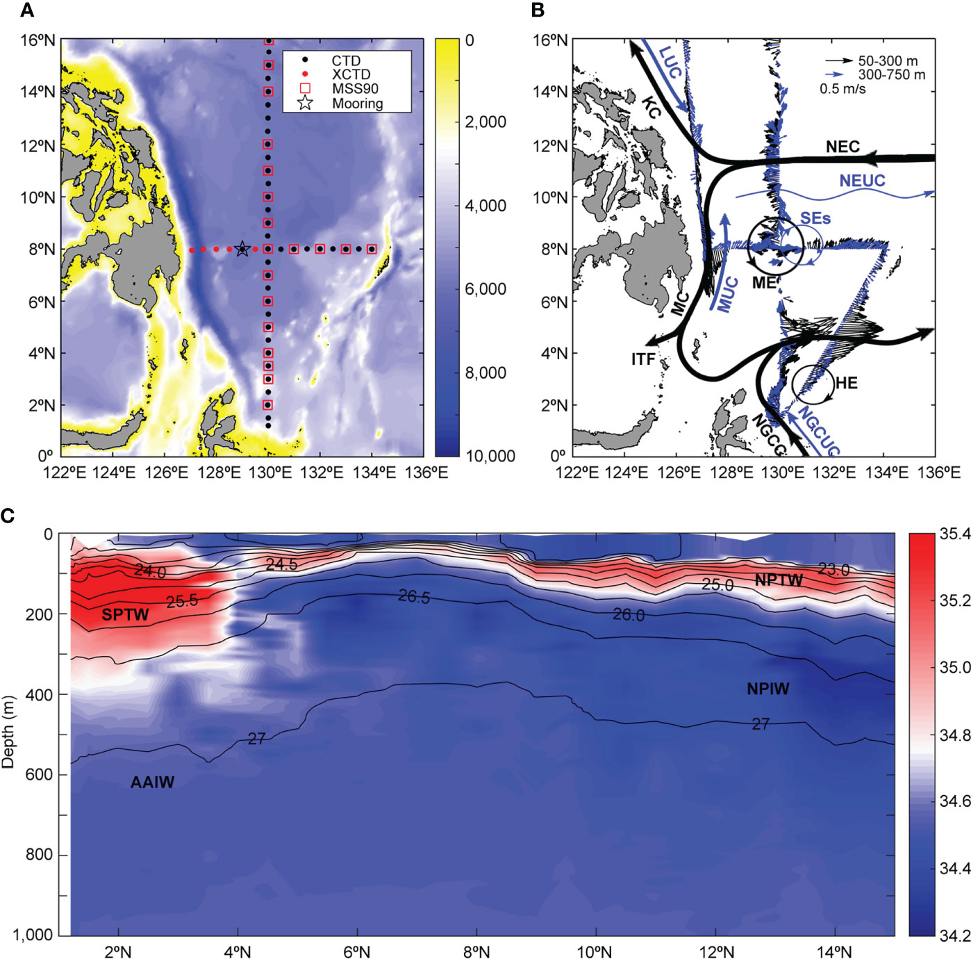
Figure 1 Observational sites, background currents, and water masses in the northwestern tropical Pacific Ocean. (A) Bathymetry and in situ observational assets. (B) Observed currents by SADCP. Major currents and eddies in the thermocline (black) and subthermocline (blue) are indicated. (C) Observed salinity (psu) along 130°E showing different water masses. The overlaying potential density σ_θ(kg m^-3) contours illustrate the distribution of stratification.

Diapycnal mixing is of crucial importance to the dynamics and thermodynamics in the WBR (Liu et al., 2017). Biases are substantial in ocean climate models due to insufficient parameterization of background diffusivity in the tropical Pacific Ocean (Zhu and Zhang, 2018). Measurement of turbulent dissipation rate was conducted recently (Liu et al., 2017). It was found that in addition to patches of enhanced mixing at eddy’s edge, mixing in the thermocline (under the mixed layer and above the main thermocline) is weak. Generally, diapycnal mixing in the ocean interior is generated by the breaking of internal gravity waves or/and shear instability of horizontal currents (Thorpe, 2005; Liu et al., 2017; Zhang et al., 2018; Zhang et al., 2019). Recent observations prove that there exist energetic subthermocline eddies (SEs) with dominant intra-seasonal variations in the WBR (Firing et al., 2005; Wang et al., 2014). Based on mooring and buoy data, our previous study showed that the SEs in the WBR play an important role in the isopycnal mixing of interhemispheric intermediate waters (Nan et al., 2019). The complex interactions among currents and SEs can provide strong shear for turbulence generation. Zhang et al. (2019) found that diapycnal mixing can be significantly elevated by a SE in the equatorial western Pacific through shear instability. In the subthermocline of the WBR, SE is energetic and stratification is relatively weak facilitating turbulence generation though shear instabilities.

To test whether diapycnal mixing can be elevated by SEs in the subthermocline of the WBR, hydrographic and microstructure observations were conducted along two perpendicular transects (Figure 1A). More than 16 months of mooring data were also obtained to investigate variabilities of SEs and associated shear changes. Based on observational data and fine-scale parameterization method, we show spatial pattern and eddy-induced variability of diapycnal mixing. The rest of the paper is organized as follows. Section 2 describes the data and methods. Section 3 presents the results on SE-induced mixing in the WBR. Section 4 discusses the importance of SE-induced mixing and summarizes the main findings.

Data and methods

Hydrographic observations

Two perpendicular transects designed to observe characteristics of currents and eddies in the WBR were carried out on board of the R/V Kexue during the period of Jan. 14^th-28^th, 2016 (Figure 1A). A total of 50 stations was sampled at ~0.5°intervals along the zonal section at 8°N and the meridional section at 130°E. Temperature and salinity profiles with 1 m vertical resolution were measured using a 911 plus conductivity-temperature-depth (CTD) manufactured by Sea-Bird Electronics Inc. and expendable CTD (XCTD) manufactured by the Tsurumi Seiki Co. Current velocities along the ship track from surface to 750 m depth are obtained using a 38 kHz SADCP with bin size of 32 m manufactured by Teledyne RD Instruments (Figure 1B). The temperature, salinity, and current data were linearly interpolated to 32-m intervals vertically between 10 m and 750 m depth. The squared buoyancy frequency representative of stratification is defined as $N^2=-\frac{g}{\rho }\frac{\partial \rho }{\partial z}$ (g is the acceleration of gravity and ρ is the potential density). The Richardson number was calculated from Ri=N²/S², where S²=(∂u/∂z)²+(∂v/∂z)² is the squared vertical shear of horizontal velocity.

Mooring data and analysis

To investigate variabilities of currents and diapycnal mixing, a subsurface mooring system (M8) was deployed in the frontal region of interhemispheric water masses at 129° E, 8° N (Figure 1A) from Jan. 14^th 2016 to Jun. 2^nd 2017. Two (one upward looking and one downward looking) 75 kHz ADCPs manufactured by Teledyne RD Instruments were mounted at ~400 m depth to measure zonal (u) and meridional (v) velocity in the upper 750 m. Quality control was performed by removing data where the percentage of good values was mostly less than 90% and in depths less than 50 m. The ADCPs were configured to measure hourly current velocity with a standard bin size of 8 m (Nan et al., 2019). The kinetic energy (KE) was calculated using KE=(u²+v²)/2. Squared shear (S²) was calculated using the vertical shear of horizontal velocity measured at the M8 mooring. Following Zhang et al. (2018), monthly temperature and salinity data, obtained from the Grid Point Value of the Monthly Objective Analysis (MOAA GPV) based on Argo profiling floats, are used to calculate stratification (N²). The MOAA GPV data is a global 1°×1° grid dataset of monthly temperature and salinity fields from January 2001 to the present (Hosoda et al., 2008). The above temperature, salinity and velocity data were all linearly interpolated to 32-m intervals vertically.

Microstructure measurement

To study mixing characteristics in the WBR, 20 sites (repeated at 130°E, 8°N) of turbulence microstructure measurements were conducted along the 8°N and 130°E sections (Figure 1A). Microstructure data were obtained using free-falling microstructure profile MSS90 manufactured by Sea and Sun Technology Instruments. The MSS 90 is a multiparameter probe for measuring turbulent velocity shear and stratification with falling velocities ranging in 0.5~0.7 m s^-1 (Lappe and Umlauf, 2016). Two shear probes sampling at 512 Hz were installed. Measured velocity shear by two shear probes are almost identical at all sites, and the mean of the dissipation estimates from the two probes was used in this analysis.

The TKE dissipation rate (ϵ_OB) was determined using the isotropic formula as in equation (1) below (Sheen et al., 2014; Bluteau et al., 2016; Liang et al., 2018),

$\begin{array}{ll}{ϵ}_{OB}=7.5\nu \overline{{\left(\frac{\partial \text{u}}{\partial z}\right)}^2}=7.5\nu \underset{0}{\overset{k_{max}}{\int }}\psi \left(k\right)dk& (1)\end{array}$

where ν is the kinematic molecular viscosity taken constant at 10^-6 m² s^-1. The overbar indicates a spatial average of the shear, u is the horizontal components of velocity, and the shear variance was calculated by integrating the spectrum of the shear signal ψ(k), where k is the vertical wavenumber (Polzin et al., 1995). The upper limit of integration k_max is the highest wavenumber not contaminated by vibration noise (Bluteau et al., 2016; Liang et al., 2018).

Dissipation rate parameterization

The maximum depth of the observed dissipation rate by the MSS90 varied and was limited to the top 400 m due to different oceanographic and weather conditions. A fine-scale parameterization method was used to estimate the dissipation rate above 750 m. There are two well-known fine-scale parameterization methods, i.e., Gregg-Henyey-Polzin (GHP) parameterization (Polzin et al., 1995; Gregg et al., 2003) and MacKinnon-Gregg (MG) parameterization (MacKinnon and Gregg, 2003 and MacKinnon and Gregg, 2005). The GHP parameterization based on internal wave-wave interaction theory has been used in the northwestern Pacific Ocean (Jing et al., 2011; Yang et al., 2014). However, it failed to predict the turbulence over rough topography (Liang et al., 2018) and overestimated diapycnal mixing in the WBR (Liu et al., 2017). The MG parameterization is found to be successful in reproducing the observed full-depth dissipation rates in the northwestern tropical Pacific (Liang et al., 2018). Thus, in this study the MG parameterization was employed. The MG dissipation rate (ϵ_MG) is expressed in terms of fine-scale shear and stratification as

$\begin{array}{ll}{\text{ϵ}}_{\text{MG}}={\text{ϵ}}_0\left(\frac{\text{N}}{{\text{ N}}_0}\right)\left(\frac{\text{S}}{{\text{ S}}_0}\right)& (2)\end{array}$

where S₀=N₀ = 0.0052 s^-1 and ϵ₀ is an constant which is set to 7.6 ×10^-9 W kg^-1 in this study to fit the parameterized dissipations best to the observed dissipations. ϵ_MGwas estimated using the 32-m resolution shear (S) and buoyancy frequency (N). Note that only ϵ_MG below the mixed layer was calculated, since in addition to eddy/current effects shears caused by wind and inertial oscillation etc. also play a vital role in the mixed layer. To evaluate the parameterization method, scatterplot of observed dissipation rate (ϵ_OB) and MG parameterized dissipation rate (ϵ_MG) were shown in Figure 2. It can be seen that the ϵ_MG pattern is close to that of the ϵ_OB. The agreement between ϵ_OB and ϵ_MG are within the same order of magnitude and about 80% of predicted ϵ_MG are within a factor of 2 of ϵ_OB, suggesting the fidelity of the MG parameterization results.

FIGURE 2

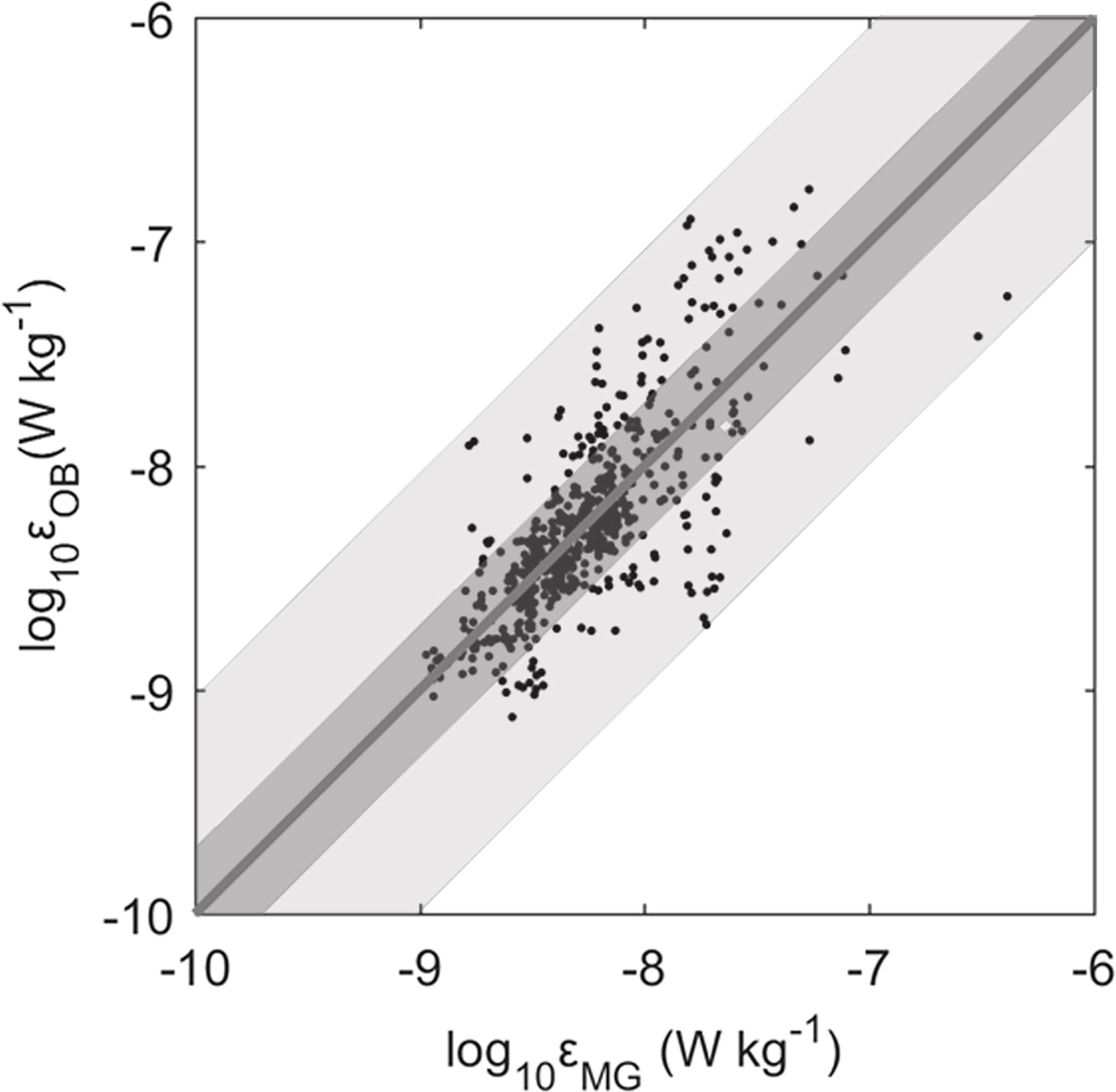
Figure 2 Comparison of observed (ϵ_OB) and parameterized (ϵ_MG) TKE dissipation rates from 20 microstructure profiles. Solid line indicates the one-to-one relations. Gray bands indicate agreement within factors of 2 and 10.

Diapycnal diffusivity representative of turbulent mixing rate is commonly estimated using the relationship κ_ρ=Γϵ/N² (Osborn, 1980), whereΓ is the mixing efficiency set to be 0.2. Note that it may be problematic using constant mixing efficiency in the mixed and bottom boundary layers (Lappe and Umlauf, 2016; Salehipour et al., 2016; Wakata, 2018; Monismith et al., 2018). However, this study focuses on the ocean interior (below the mixed layer and far away from the bottom boundary layer). Thus, constant mixing efficiency was reserved.

Results

Observations of SEs

The main currents and eddies are captured in the WBR by the ship-mounted Acoustic Doppler Current Profilers (SADCP) in the winter of 2016 (Figure 1B and Figure 3). It can be seen that the NEC flows westward between 7°N and 16°N with a maximum speed larger than 0.5 m s^-1. Most part of the NEC is above the main thermocline. However, there are small branches can reach 750 m. The NECC flows eastward between 2°N and 6°N with maximum speed larger than 1 m s^-1. Westward NEC and eastward NECC cause divergence between 5°N and 9°N which uplifts the thermocline by ~100 m (Figure 1C). The MC flows southward along the east Philippine coast (west of 129 °E) with maximum speed larger than 1 m/s. The southward MUC located below the MC were not totally captured limited by observational depth.

FIGURE 3

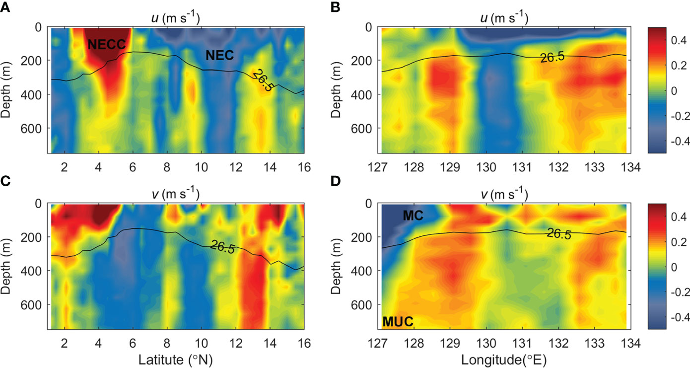
Figure 3 (A, C), Zonal (u) and meridional (v) velocities along the 130°E section measured by the SADCP. (B, D), Similar to (A, C) but for the 8°N section. Contours of 26.5 kg m^-3 are shown to indicate the main thermocline depth.

The most striking feature of Figure 3 is that in addition to the main currents, there are also subtermocline currents and SEs. For example, there is an anticylonic SE between 128°E and 131°E at the 8°N section (Figure 3B). It has subsurface-intensified core located at 200~750 m depth with maximum swirl speed of 0.4 m s^-1. To observe variations of the SEs, a subsurface mooring system (M8) was deployed for 16.5 months in the frontal region of interhemispheric water masses at 129° E, 8° N (Figure 1A). Hourly zonal (u) and meridional (v) velocities were obtained in the 50-750 m layer (Figure 4). As shown before, the main thermocline (~26.5 σ_θ) depth is shallower and located at about 200 m depth at the M8 mooring site. It can be seen that the SEs are located between 200 and 750 m (Figure 5A) with a maximum swirl speed reaching 0.5 m s^-1. The power spectrum for KE averaged between 200 and 750 m shows that the SEs in this region exhibit intra-seasonal variability with the period ranging between 50 and 100 days (Figure 6). The power is greatest at 90 days. There are both cyclonic and anticyclonic SEs, whose vertical structures have been shown in Figure 2C of Nan et al. (2019). Several SEs passed by the mooring during the observation period (Figure 5A). The formation of SEs, which has been attributed to both barotropic and baroclinic instabilities (Chiang and Qu, 2013; Chiang et al., 2015), is not studied here due to limited observational data. However, the strong velocity shear forms due to interactions among currents and eddies, which tends to contribute to turbulence generation.

FIGURE 4

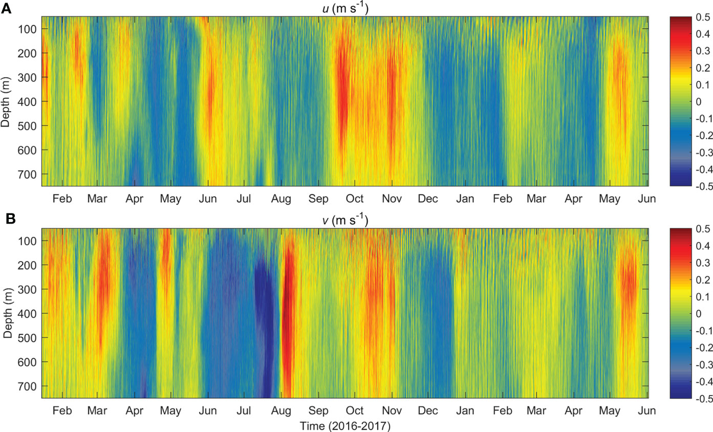
Figure 4 Hourly (A) zonal (u) and (B) meridional (v) velocity measured at the M8 mooring from Jan. 14^th, 2016 to Jun. 2^nd, 2017.

FIGURE 5

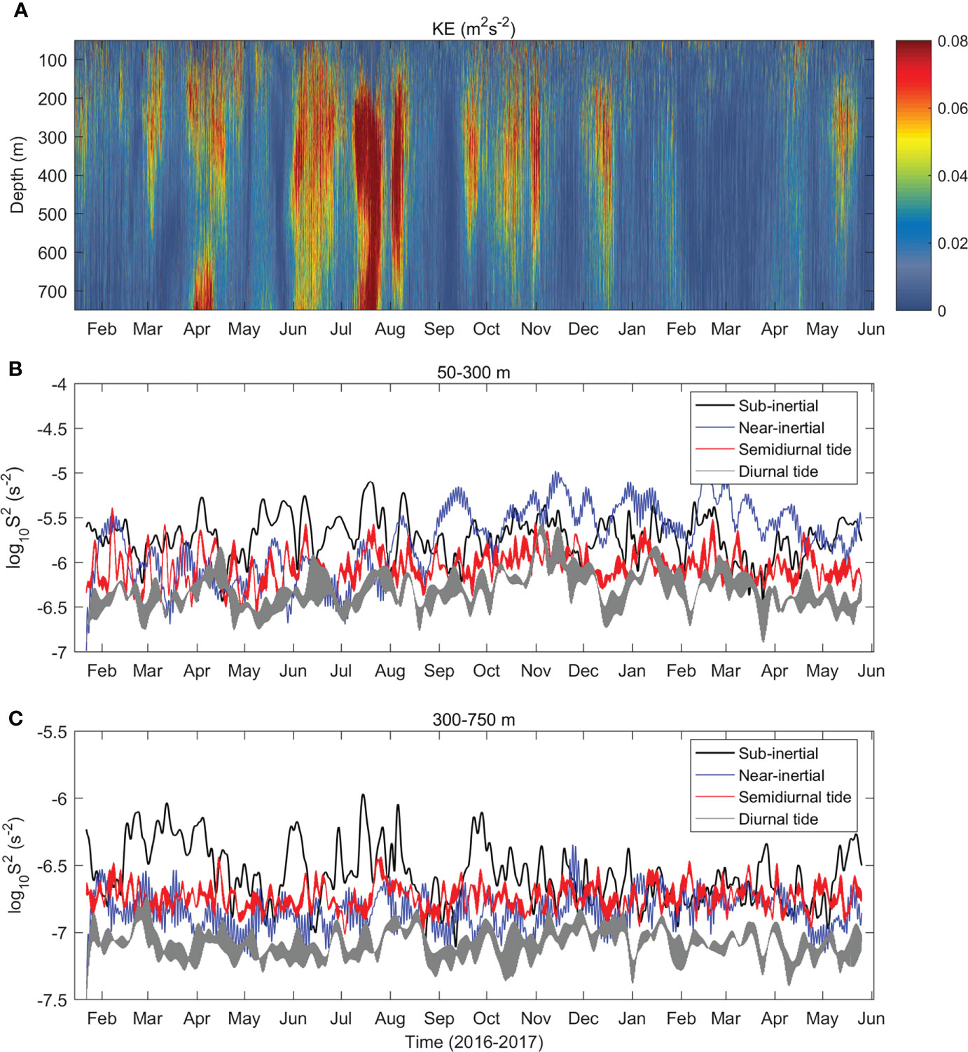
Figure 5 (A) Hourly profiles of measured KE at the M8 mooring. (B, C), Time series of squared shear (S²) divided into semidiunal tide, diurnal tide, near-inertial, and sub-inertial frequency bands and averaged for 50-200 m and 200-750 m, respectively.

FIGURE 6

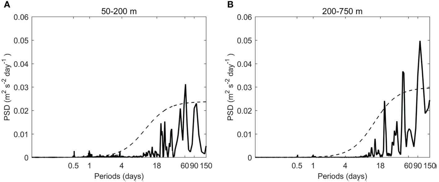
Figure 6 PSD of hourly KE averaged for 50-200 m (A) and 200-750 m (B) at the M8 mooring, respectively. The dashed lines denote the 95% significance level.

Spatial structure of diapycnal mixing

To characterize the diapycnal mixing in the WBR, microstructure data were obtained at 20 sites along the 8°N and 130°E sections (Figure 1A) in the winter of 2016. The depths at these sites exceed 2000 m, and the microstructure measurements in the upper 400 m are far away from direct influences of the bottom. The turbulent kinetic energy (TKE) dissipation rate (ϵ_OB) was calculated (see Methods) along the two sections (Figures 7A, B). It can be seen that the TKE dissipation rate ranges from 10^-10 W kg^-1 to 10^-6 W kg^-1 exhibiting nonuniform distributions either horizontally or vertically. Generally, the TKE dissipation rate decreases with depth. It is the largest in the mixed layer with a mean dissipation rate of 4.6× 10^-7 W kg^-1. Consistent with the TKE dissipation rate, the velocity shear is the largest in the mixed layer and decreases with depth. Correspondingly, the diapycnal diffusivity (κ_ρ) representative of mixing rate is almost always larger than 10^-4 m² s^-1 in the mixed layer (Figures 7C, D). Not surprisingly, mixing is the strongest in the mixed layer, which is induced by wind stirring, wave breaking, inertial oscillations, and/or positive buoyancy fluxes as in many other regions (Munk, 1966; Thorpe, 2005; Liu et al., 2017).

FIGURE 7

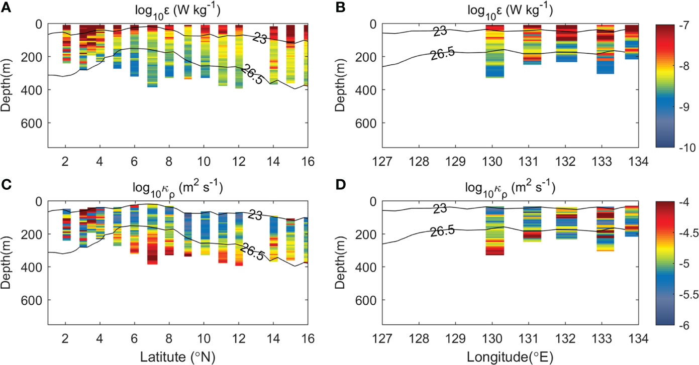
Figure 7 (A, C), Observed dissipation rate and diapycnal diffusivity (κ_ρ) along the 130°E section, respectively. (B, D), Similar to (A, C) but for the 8°N section. Contours of σ_θ = 23 and 26.5 kg m^-3 are shown to indicate the mixed layer depth and the main thermocline depth, respectively.

In the thermocline and subthermocline layers there are patches of enhanced TKE dissipation rates (Figures 7C, D). These enhanced patches are consistent with the patchy shears induced by currents or eddies (Figure 4). Different from the decreasing of TKE dissipation rates with depth, the diapycnal diffusivity (κ_ρ) increased with depth due to weak stratification. In the thermocline, although there are patches of large diapycnal diffusivity, such as at the south edge of the NECC between 2°N and 4°N, the diapycnal diffusivities (κ_ρ) are on the order of 10^-6~10^-5 m² s^-1, i.e., at the background values in the open ocean (Waterhouse et al., 2014; Liu et al., 2017). Previous observations in the summer of 2014 also show that excluding the eddy enhanced patches, diapycnal mixing in the thermocline is generally weak with diapycnal diffusivity κ_ρ~Ο(10^-6) m² s^-1 (Liu et al., 2017). It is known that eddies can enhance diapycnal diffusivity at its edges due to geostrophic shear (Fine et al., 1994; Liu et al., 2017; Yang et al., 2017). Based on the MG parameterization (Figure 8), diapycnal diffusivity in the subthermocline was calculated at the 20 observational sites. Strikingly, the diapycnal diffusivity increased up to 2.66×10^-4 m² s^-1 at 750 m (Figure 9). The mean diapycnal diffusivity κ_ρis 0.75×10^-4 m² s^-1 in the subthermocline larger than that in the thermocline by a factor of four. The standard deviation of κ_ρ is 0.60×10^-4 m² s^-1 comparable with the mean value, indicating that eddy-induced variation of mixing is significant. Limited by observational data, the increase of diapycnal diffusivity below 750 m due to SEs was not fully captured.

FIGURE 8

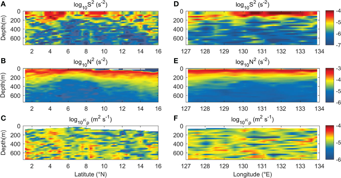
Figure 8 (A–C), Squared shear (S²), squared buoyancy frequency (N²), and diapycnal diffusivity (κ_ρ) derived from parameterized (ϵ_MG) TKE dissipation rates along the 130°E section. (D–F), Similar to (A–C) but for the 8°N section.

FIGURE 9

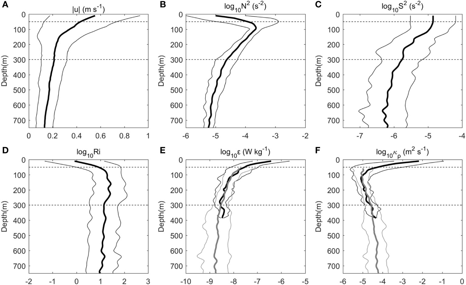
Figure 9 Vertical distributions (thick lines) of the averaged current speed (A), squared buoyancy frequency (N²) (B), squared shear (S²) (C), Richardson number (Ri) (D), dissipation rate (ϵ) (E), diapycnal diffusivity (κ_ρ) (F), and its standard deviations (thin lines) at 20 microstructure profiles. Dotted lines at 50 m and 300 m indicate the mixed layer and the main thermocline depths, respectively. Gray lines in (E, F) represent results of MG parameterization.

It is argued that the weak thermocline mixing in the WBR is caused by reduced breaking of internal waves (Gregg et al., 2003; Liu et al., 2017). From Figures 8A, D, shear in the thermocline is larger than that in the subthermocline. However, the stratification is strongest in the thermocline indicated by the squared buoyancy frequency (N²) (Figures 8B and 9E). In the subthermocline, direct influences of the surface or bottom boundaries are insignificant. Relatively weak stratification favors turbulence generation whenever the shear is present (e.g., in cases of energetic SEs, Figures 8A, B) to facilitate instabilities. The most striking feature of spatial structure of diapycnal mixing in the study region is that it has a sandwich-like structure above 750 m with weak mixing in the thermocline and strong mixing in the mixed layer and subthermocline.

SE-induced variability of diapycnal mixing

Case studies show that eddies can enhance diapycnal mixing at its edges (Liu et al., 2017; Yang et al., 2017; Fine et al., 2018; Zhang et al., 2019; Cao et al., 2022). However, temporal variability of diapycnal mixing induced by SEs remains unclear. At the M8 mooring site, the main thermocline is uplifted to ~200 m depth due to divergence caused by westward NEC and eastward NECC (Figure 3). Thus, 200 m was selected to separate the thermocline layer and the subthermocline layer at the mooring site. Power spectra for hourly KE show that there are significant contributions from semi-diurnal tide currents, diurnal tide currents, and sub-inertial currents both in the thermocline (50-200 m) and in the subthermocline (200-750 m) (Figure 6). Among them, sub-inertial currents representative of eddy activities dominate with periods between 18 and 120 days. In the thermocline, there is also near-inertial current with period close to the local inertial period (T_i) of 3.58 days. Note that large current velocity does not mean that the associated shear is large. To obtain frequency-dependent components of S², measured velocity are decomposed into different frequency bands using the third-order Butterworth filter. Specifically, the velocities within the semi-diurnal, diurnal, and near-inertial bands were band-pass filtered with cutoff periods at 10-14 h, 20-27 h, and (0.80-1.18)T_i, respectively (Zhang et al., 2018). T_i (3.58 days) represents the local inertial period at 8°N. For the sub-inertial velocity, it was obtained via low-pass filtering with cutoff periods of 18 days following the previous study (Zhang et al., 2018). Time series of squared shear (S²) in the semi-diurnal tide, diurnal tide, near-inertial, and sub-inertial frequency bands averaged for 50-200 m and 200-750 m are showed in Figure 5B and Figure 5C, respectively. It can be seen that shears induced by near-inertial and sub-inertial currents are dominant in the thermocline. In the subthermocline, shear induced by near-inertial currents is weak, while shear induced by sub-inertial currents remains dominant. Compared with shear induced by near-inertial and sub-inertial currents, shear induced by tidal currents is smaller.

Several SEs passed by the mooring site during our observational period (Figure 10A). If identified by velocity contours larger than 0.1 m s^-1, the SE occurrence at the mooring site can reach 79%. The shear variations exhibit a significant correlation with sub-inertial KE. The correlation coefficient between sub-inertial KE and diapycnal diffusivity is 0.62 exceeding 99% significance level, when sub-inertial KE lags diapycnal diffusivity by ~5 days (Figure 10). Peak-to-peak comparisons also show that variation of diapycnal diffusivity leads that of sub-inertial KE. This is because that SEs enhance shear at the edges but not the positions of maximum velocity/KE (Liu et al., 2017; Yang et al., 2017). Based on modeling results, it has been shown that most SEs east of the Philippines propagate westward (Chiang and Qu, 2013). The 5-day lag reflects that the maximum shear formed when the SEs approach the mooring and before the maximum KE appears. It can be seen that the shear was elevated by up to two orders of magnitude when the SEs passed the mooring (Figure 10B).

FIGURE 10

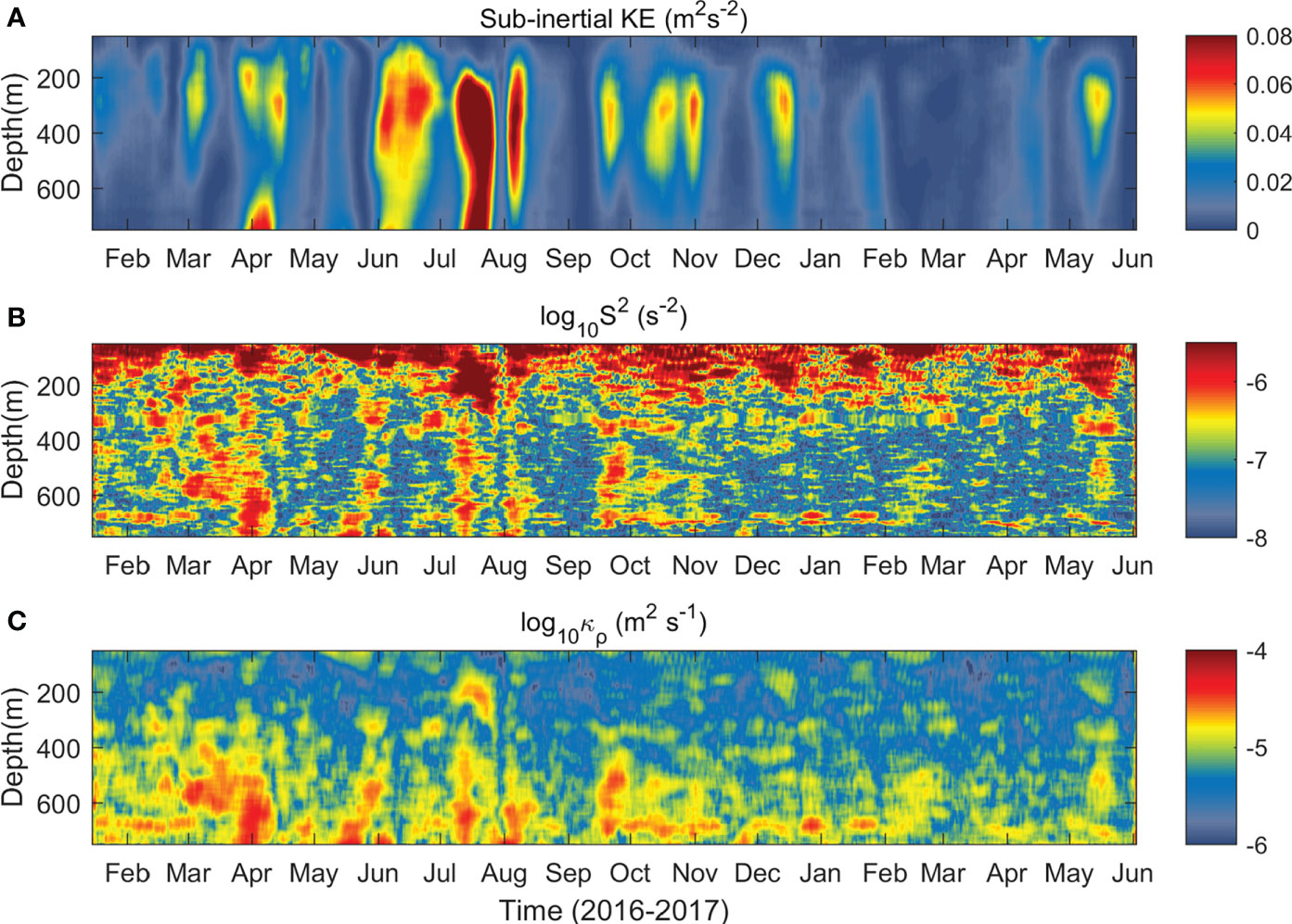
Figure 10 Variabilities of measured sub-inertial KE (A), associated squared shear (S²) (B), and estimated diapycnal diffusivity (κ_ρ) (C) based on MG parameterization at the M8 mooring.

Based on the shear induced by the SEs, variabilities of diapycnal diffusivity (κ_ρ) was estimated using the MG parameterization (Figure 10C). Diapycnal diffusivity increases with depth ranging from 10^-6 m² s^-1 to 10^-4 m² s^-1, which is consistent with the result shown in Figures 8C and 8F. Although there exists strong shear in the thermocline (Figure 10B), diapycnal mixing is mostly weak, suppressed by strong stratification (Figure 11A). In the subthermocline, diapycnal diffusivity is elevated by one order, up to 10^-4 m² s^-1 when the SEs pass by the mooring site (Figure 10C). The integrated diapycnal diffusivity between 200 and 750 m is increased by 210% (Figure 12). Note that stratification is derived from the monthly Argo data. Thus, the value (210%) of diapycnal diffusivity increased by the SEs maybe underestimated. Elevated diapycnal diffusivities correlate well with that of low Ri (Figure 11B). The correlation coefficient between diapycnal diffusivity and shear is 0.98 exceeding 99% significance level (Figure 12C). It is not surprising that the shear modulated by the SEs exhibits intra-seasonal variabilities with periods ranging from 18 to 120 days (Figure 13A). Thus, given the strong correlation, the diapycnal mixing in the subthermocline at the mooring site also has significant intra-seasonal variations (Figure 13B).

FIGURE 11

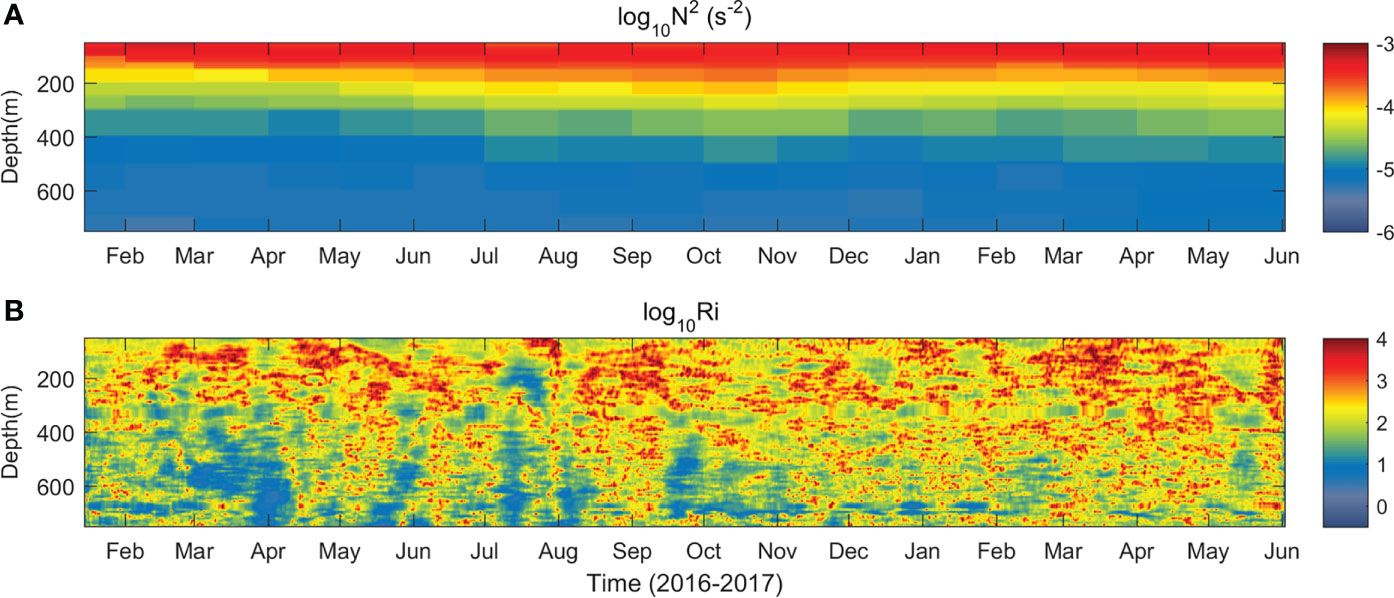
Figure 11 Time series of (A) squared buoyancy frequency (N²) from monthly Argo data, and (B) Richardson number (Ri) at the M8 mooring.

FIGURE 12

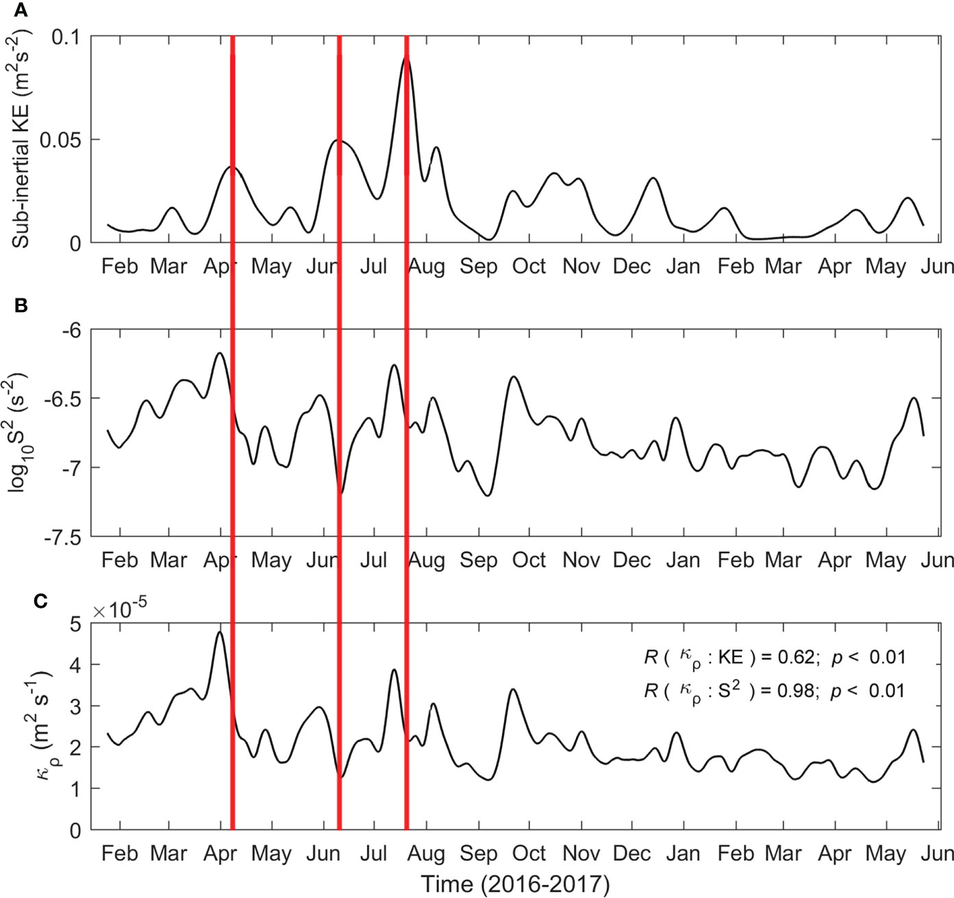
Figure 12 Variabilities of measured sub-inertial KE (A), associated squared shear (S²) (B), and estimated diapycnal diffusivity (κ_ρ) (C) based on MG parameterization averaged for 200~750 m at the M8 mooring. The red solid lines shows central position of three strong SEs.

FIGURE 13

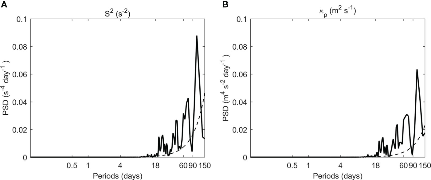
Figure 13 PSD of hourly squared shear (S²) (A) and diapycnal diffusivity (κ_ρ) (B) averaged for 200-750 m at the M8 mooring site, respectively. The dashed lines denote the 95% significance level.

Summary and discussion

In summary, this study presents the observational evidences of the SE-induced spatial structure and variability of diapycnal mixing in the WBR. The SEs are located between 200 and 750 m with a maximum swirl speed reaching 0.5 m s^-1 and exhibit intra-seasonal variability with the period ranging between 50 and 100 days. Compared with shears induced by tides and near-inertial oscillation, SE-induced sub-inertial shears are dominant in the subthermocline layer. Consequently, diapycnal mixing is elevated by up to one order of magnitude compared to the background value due to relatively weak stratification and incresed shear induced by SEs. Because of the successive arrival of SEs, diapycnal mixing in the subthermocline has significant intreaseasonal variations.

Diapycnal mixing has a strong impact on the transformation of interhemispheric water masses in the WBR and hence on the tropical overturning circulation (Fine et al., 1994; Furue and Endoh, 2005; Zhu and Zhang, 2018). The SEs play an important role on the variation of diapycnal mixing in the subthermocline layer. It has been argued that an average diapycnal diffusivity κ_ρ~O(10^-4) m² s^-1 is required to maintain the stratification and drive the meridional overturning circulation (Munk, 1966; Munk and Wunsch, 1998). However, diapycnal diffusivity cannot reach 10^-4 m² s^-1 in the interior of the most world’s open ocean. With more and more subthermocline eddies being observed around the global ocean (Pelland et al., 2013; Zhang et al., 2015; Dilmahamod et al., 2018), diapycnal mixing in the subthermocline layer may supply part of the “missing” mixing in the ocean interior. We speculate that a similar picture may apply to other regions where SEs are active. It is worth noting that our observations are limited to above the 750 m depth. More observations targeted on SE-induced mixing are called for.

In a previous study, we investigated the SE effect on isopycnal mixing of interhemispheric water masses in the WBR (Nan et al., 2019). It was found that the horizontal eddy diffusivity has subthermocline maxima induced by SEs off the Philippine coast. Thus, SEs play an important role in both isopycnal and diapycnal mixings of water masses in the study region. Diapycnal mixing effects cannot be resolved by ocean climate models, and instead have to be parameterized. Constant diffusivity value is often used in numerical ocean models (Furue and Endoh, 2005; Koch-Larrouy et al., 2007; Cole et al., 2015), and as a result, biases are substantial in ocean climate models in the tropical Pacific Ocean (Zhu et al., 2018). Our findings in this study suggest that the vertically varying diapycnal diffusivity should be used to improve parameterization of diapycnal mixing in the tropical northwestern Pacific in ocean climate models.

Data availability statement

The datasets presented in this study can be found in online repositories. The names of the repository/repositories and accession number(s) can be found below: http://www.jamstec.go.jp/ARGO/argo_web/argo/?lang=en The observational data supporting the findings of this study are available from the corresponding author upon request (yuf@qdio.ac.cn).

Author contributions

FN, HX and FY conceived the research. QR designed the mooring at 129°E, 8°N and processed the mooring data. JW processed the microstructure data. FN conducted data analysis and wrote the first draft of the paper with all the authors’ contribution to the revisions. All authors contributed to the article and approved the submitted version.

Acknowledgments

The authors would like to thank the crew and technicians on the R/V Kexue of Institute of Oceanology, Chinese Academy of Sciences, for their valuable assistance with mooring deployment and retrieval. This work was jointly supported by the National Natural Science Foundation of China (41676005), MEL Visiting Fellowship (MELRS2217), Youth Innovation Promotion Association of CAS and the Global Climate Changes and Air-sea Interaction Program (GASI-02-PAC-ST-Wwin).

Conflict of interest

The authors declare that the research was conducted in the absence of any commercial or financial relationships that could be construed as a potential conflict of interest.

Publisher’s Note

All claims expressed in this article are solely those of the authors and do not necessarily represent those of their affiliated organizations, or those of the publisher, the editors and the reviewers. Any product that may be evaluated in this article, or claim that may be made by its manufacturer, is not guaranteed or endorsed by the publisher.

References

Bluteau C. E., Jones N. L., Ivey G. N. (2016). Estimating turbulent dissipation from microstructure shear measurements using maximum likelihood spectral fitting over the inertial and viscous subranges. J. Atmos. Oceanic Technol. 33, 713–722. doi: 10.1175/JTECH-D-15-0218.1

CrossRef Full Text | Google Scholar

Cao A. Z., Liu C., Chen J., Li P. L., Song J. B. (2022). Enhanced turbulent mixing in mesoscale eddies near the critical latitude of the M2 internal tides. Deep–Sea Res. I. 185, 103801. doi: 10.1016/j.dsr.2022.103801

CrossRef Full Text | Google Scholar

Chen L., Jia Y., Liu Q. (2015). Mesoscale eddies in the Mindanao dome region. J. oceanography 71 (1), 133–140. doi: 10.1007/s10872-014-0255-3

CrossRef Full Text | Google Scholar

Chiang T. L., Qu T. (2013). Subthermocline eddies in the western equatorial pacific as shown by an eddy-resolving OGCM. J. Phys. Oceanography 43 (7), 1241–1253. doi: 10.1175/JPO-D-12-0187.1

CrossRef Full Text | Google Scholar

Chiang T.-L., Wu C.-R., Qu T., Hsin Y.-C. (2015). Activities of 50-80 day subthermocline eddies near the Philippine coast. J. Geophys. Res. Oceans 120, 3606–3623. doi: 10.1002/2013JC009626

CrossRef Full Text | Google Scholar

Cole S. T., Wortham C., Kunze E., Owens W. B. (2015). Eddy stirring and horizontal diffusivity from argo float observations: Geographic and depth variability. Geophys. Res. Lett. 42, 3989–3997. doi: 10.1002/2015GL063827

CrossRef Full Text | Google Scholar

Dilmahamod A., Aguiar-González B., Penven P., Reason C. J. C., De Ruijter W. P. M., Malan N., et al. (2018). SIDDIES corridor: A major East-West pathway of long-lived surface and subsurface eddies crossing the subtropical south Indian ocean. J. Geophysical Research: Oceans 123 (2), 5406–5425. doi: 10.1029/2018JC013828

CrossRef Full Text | Google Scholar

Fine R. A., Lukas R., Bingham F. M., Warner M. J., Gammon R. H. (1994). The western equatorial pacific: A water mass crossroads. J. Geophysical Res. Oceans 99 (12), 25063–25080. doi: 10.1029/94JC02277

CrossRef Full Text | Google Scholar

Fine E. C., MacKinnon J. A., Alford M. H., Mickett J. B. (2018). Microstructure observations of turbulent heat fluxes in a warm-core Canada basin eddy. J. Phys. Oceanogr. 48, 2397–2418. doi: 10.1175/JPO-D-18-0028.1

CrossRef Full Text | Google Scholar

Firing E., Kashino Y., Hacker P. (2005). Energetic subthermocline currents observed east of Mindanao. Deep Sea Res. Part II 52 (3-4), 605–613. doi: 10.1016/j.dsr2.2004.12.007

CrossRef Full Text | Google Scholar

Furue R., Endoh M. (2005). Effects of the pacific diapycnal mixing and wind stress on the global and pacific meridional overturning circulation. J. Phys. Oceanogr. 35, 1876–1890. doi: 10.1175/JPO2792.1

CrossRef Full Text | Google Scholar

Gregg M. (1987). Diapycnal mixing in the thermocline. J. Geophys. Res. 92 (5), 5249–5286. doi: 10.1029/JC092iC05p05249

CrossRef Full Text | Google Scholar

Gregg M. C., Sanford T. B., Winkel D. P. (2003). Reduced mixing from the breaking of internal waves in equatorial waters. Nature 422, 513–515. doi: 10.1038/nature01507

PubMed Abstract | CrossRef Full Text | Google Scholar

Grenier M., Cravatte S., Blanke B., Menkes C., Koch-Larrouy A., Durand F., et al. (2011). From the western boundary currents to the pacific equatorial undercurrent: Modeled pathways and water mass evolutions. J. Geophysical Res. 116, C12044. doi: 10.1029/2011JC007477

CrossRef Full Text | Google Scholar

Hosoda S., Ohira T., Nakamura T. (2008). A monthly mean dataset of global oceanic temperature and salinity derived from argo float observations. JAMSTEC Rep. Res. Dev. 8, 47–59. doi: 10.5918/jamstecr.8.47

CrossRef Full Text | Google Scholar

Hu D. X., Wu L. X., Cai W. J., Sen Gupta A., Ganachaud A., Qiu B., et al. (2015). Pacific western boundary currents and their roles in climate. Nature 522, 299–308. doi: 10.1038/nature14504

PubMed Abstract | CrossRef Full Text | Google Scholar

Jing Z., Wu L., Li L., Liu C., Liang X., Chen Z., et al. (2011). Turbulent diapycnal mixing in the subtropical northwestern pacific: Spatial-seasonal variations and role of eddies. J. Geophys Res-Oceans 116, C10028. doi: 10.1029/2011JC007142

CrossRef Full Text | Google Scholar

Kashino Y., Atmadipoera A., Kuroda Y. (2013). Observed features of the halmahera and Mindanao eddies. J. Geophys. Res. Oceans 118, 6543–6560. doi: 10.1002/2013JC009207

CrossRef Full Text | Google Scholar

Koch-Larrouy A., Madec G., Bouruet-Aubertot P., Gerkema T., Bessières L., Molcard R. (2007). On the transformation of pacific water into Indonesian throughflow water by internal tidal mixing. Geophys. Res. Lett. 34, L04604. doi: 10.1029/2006GL028405

CrossRef Full Text | Google Scholar

Lappe C., Umlauf L. (2016). Efficient boundary mixing due to near-inertial waves in a nontidal basin: Observations from the Baltic Sea. J. Geophys. Res. Oceans 121, 8287–8304. doi: 10.1002/2016JC011985

CrossRef Full Text | Google Scholar

Ledwell J., Watson A., Law C. (1993). Evidence for slow mixing across the pycnocline from an open-ocean tracer-release experiment. Nature 364, 701–703. doi: 10.1038/364701a0

CrossRef Full Text | Google Scholar

Liang C., Shang X., Qi Y., Chen G., Yu L. (2018). Assessment of fine-scale parameterizations at low latitudes of the north pacific. Sci. Rep. 8, 10281. doi: 10.1038/s41598-018-28554-z

PubMed Abstract | CrossRef Full Text | Google Scholar

Liu Z., Lian Q., Zhang F., Wang L., Li M., Bai X., et al. (2017). Weak thermocline mixing in the north pacific low-latitude western boundary current system. Geophysical Res. Lett. 44, 10,530–10,539. doi: 10.1002/2017GL075210

CrossRef Full Text | Google Scholar

MacKinnon J. A., Gregg M. C. (2003). Mixing on the late-summer new England shelf–solibores, shear, and stratification. J. Phys. Oceanogr. 33 (7), 1476–1492. doi: 10.1175/1520-0485(2003)033<1476:MOTLNE>2.0.CO;2

CrossRef Full Text | Google Scholar

MacKinnon J. A., Gregg M. C. (2005). Near-inertial waves on the new England shelf: The role of evolving stratification, turbulent dissipation, and bottom drag. J. Phys. Oceanogr. 35, 2408–2424. doi: 10.1175/JPO2822.1

CrossRef Full Text | Google Scholar

Monismith S. G., Koseff J. R., White B. L. (2018). Mixing efficiency in the presence of stratification: when is it constant? Geophysical Res. Lett. 45 (11), 5627–5634. doi: 10.1029/2018GL077229

CrossRef Full Text | Google Scholar

Munk W. H. (1966). Abyssal recipes. Deep-Sea Res. 13, 707–730. doi: 10.1016/0011-7471(66)90602-4

CrossRef Full Text | Google Scholar

Munk W., Wunsch C. (1998). Abyssal recipes II: Energetics of tidal and wind mixing. Deep-Sea Res. Part I 45, 1977–2010. doi: 10.1016/S0967-0637(98)00070-3

CrossRef Full Text | Google Scholar

Nan F., Yu F., Ren Q., Wei C., Liu Y., Sun S. (2019). Isopycnal mixing of interhemispheric intermediate waters by subthermocline eddies east of the Philippines. Sci. Rep. 9, 2957. doi: 10.1038/s41598-019-39596-2

PubMed Abstract | CrossRef Full Text | Google Scholar

Nan F., Yu F., Xue H., Wang R., Si G. (2015). Ocean salinity changes in the northwest pacific subtropical gyre: the quasi-decadal oscillation and the freshening trend. J. Geophys. Res. Oceans 120, 2179–2192. doi: 10.1002/2014JC010536

CrossRef Full Text | Google Scholar

Osborn T. (1980). Estimates of the local rate of vertical diffusion from dissipation measurements. J. Phys. Oceanography 10 (1), 83–89. doi: 10.1175/1520-0485(1980)010<0083:EOTLRO>2.0.CO;2

CrossRef Full Text | Google Scholar

Pelland N., Eriksen C., Lee C. (2013). Subthermocline eddies over the Washington continental slope as observed by seagliders 2003-09. J. Phys. Oceanogr. 43, 2025–2053. doi: 10.1175/JPO-D-12-086.1

CrossRef Full Text | Google Scholar

Polzin K. L., Toole J. M., Schmitt R. W. (1995). Finescale parameterizations of turbulent dissipation. J. Phys. Oceanogr. 25, 306–328. doi: 10.1175/1520-0485(1995)025<0306:FPOTD>2.0.CO;2

CrossRef Full Text | Google Scholar

Qiu B., Chen S., Rudnick D. L., Kashino Y. (2015). A new paradigm for the north pacific subthermocline low-latitude western boundary current system. J. Phys. Oceanography 45 (9), 2407–2423. doi: 10.1175/JPO-D-15-0035.1

CrossRef Full Text | Google Scholar

Salehipour H., Peltier W. R., Whalen C. B., MacKinnon J. A. (2016). A new characterization of the turbulent diapycnal diffusivities of mass and momentum in the ocean. Geophys. Res. Lett. 43, 3370–3379. doi: 10.1002/2016GL068184

CrossRef Full Text | Google Scholar

Schönau M. C., Rudnick D. L. (2017). Mindanao Current and undercurrent: Thermohaline structure and transport from repeat glider observations. J. Phys. Oceanography 47 (8), 2055–2075. doi: 10.1175/JPO-D-16-0274.1

CrossRef Full Text | Google Scholar

Sheen K. L., Garabato A. N., Brearley J. A., Meredith M. P., Polzin K. L., Smeed D. A., et al. (2014). M. eddy-induced variability in southern ocean abyssal mixing on climatic timescales. Nat. Geosci. 7 (8), 577. doi: 10.1038/ngeo2200

CrossRef Full Text | Google Scholar

Thorpe S. A. (2005). The turbulent ocean (Cambridge: Cambridge University Press), 345–357.

Google Scholar

Wakata Y. (2018). LES study of vertical eddy diffusivity estimation in bottom boundary layers. J. Phys. Oceanogr. 48, 1903–1920. doi: 10.1175/JPO-D-17-0165.1

CrossRef Full Text | Google Scholar

Wang Q., Zhai F., Wang F., Hu D. (2014). Intraseasonal variability of the subthermocline current east of Mindanao. J. Geophysical Research: Oceans 119 (12), 8552–8566. doi: 10.1002/2014JC010343

CrossRef Full Text | Google Scholar

Waterhouse A. F., MacKinnon J. A., Nash J. D., Alford M. H., Kunze E., Simmons H. L., et al. (2014). Global patterns of diapycnal mixing from measurements of the turbulent dissipation rate. J. Phys. Oceanography 44 (7), 1854–1872. doi: 10.1175/JPO-D-13-0104.1

CrossRef Full Text | Google Scholar

Wunsch C., Ferrari R. (2004). Vertical mixing, energy, and the general circulation of the oceans. Annu. Rev. Fluid Mech. 36, 281–314. doi: 10.1146/annurev.fluid.36.050802.122121

CrossRef Full Text | Google Scholar

Yang Q., Zhao W., Liang X., Dong J., Tian J. (2017). Elevated mixing in the periphery of mesoscale eddies in the south China Sea. J. Phys. Oceanogr. 47, 895–907. doi: 10.1175/JPO-D-16-0256.1

CrossRef Full Text | Google Scholar

Yang Q., Zhao W., Li M., Tian J. (2014). Spatial structure of turbulent mixing in the northwestern pacific ocean. J. Phys. Oceanography 44 (8), 2235–2247. doi: 10.1175/JPO-D-13-0148.1

CrossRef Full Text | Google Scholar

Zhang Z., Liu Z., Richards K., Shang G., Zhao W., Tian J., et al. (2019). Elevated diapycnal mixing by a subthermocline eddy in the western equatorial pacific. Geophysical Res. Lett. 46, 2628–2636. doi: 10.1029/2018GL081512

CrossRef Full Text | Google Scholar

Zhang Z., Li C., Zhao W., Tian J., Qu T. (2015). Subthermocline eddies observed by rapid-sampling argo floats in the subtropical northwestern pacific ocean in spring 2014. Geophys. Res. Lett. 42, 6438–6445. doi: 10.1002/2015GL064601

CrossRef Full Text | Google Scholar

Zhang Z., Qiu B., Tian J., Zhao W., Huang X. (2018). Latitude-dependent finescale turbulent shear generations in the pacific tropical-extratropical upper ocean. Nat. Commun. 9 (1), 4086. doi: 10.1038/s41467-018-06260-8

PubMed Abstract | CrossRef Full Text | Google Scholar

Zhang L., Wang F. J., Wang Q., Hu S., Wang F., Hu D. (2017). Structure and variability of the north equatorial Current/Undercurrent from mooring measurements at 130° e in the Western pacific. Sci. Rep. 7, 46310. doi: 10.1038/srep46310

PubMed Abstract | CrossRef Full Text | Google Scholar

Zhu Y., Zhang R.-H. (2018). An argo-derived background diffusivity parameterization for improved ocean simulations in the tropical pacific. Geophysical Res. Lett. 45, 1509–1517. doi: 10.1002/2017GL076269

CrossRef Full Text | Google Scholar