Measurement principle and technology of miniaturized strapdown inertial wave sensor

This paper presents the design and implementation of a low-cost directional inertial wave sensor, DWS19-2, which is suitable for installation on ocean air-sea coupling buoys, offshore environmental monitoring buoys and surface drifting buoys. DWS19-2 integrates an STM32F446 embedded controller with a 9-axis MEMS inertial module QZ901 to measure buoy pitch, roll, heading and accelerations. These parameters are further used to calculate wave parameters and estimate directional and non-directional wave spectra. These wave parameters and spectral information are then reported to the buoy data logger for real-time transmission to shore-based data centers. Details of the electrical design and onboard wave processing algorithm (coordinate projection, numerical integration in the frequency domain, time-based wave parameters, frequency-based wave parameters, directional wave spectrum), in addition to turntable tests, filed marine comparison with DWR-MKIII wave buoy and related ocean observation applications enabled by this device, are described in this paper.

Introduction

In the field of ocean wave observations, inertial wave measurements have been a major method for observing ocean waves ever since their invention. Its advantages over pressure gauges, acoustic sensors, and laser remote sensors are made possible by not being affected by water depth and field mounting environment (Doong et al., 2011; Qi et al., 2019). Wave sensors have gradually developed toward miniaturization, low power consumption, and low-cost to meet the increasing requirements of mobile and portable observations (Datawell; TRIAXYSy). The South China Sea Institute of Oceanology (SCSIO), Chinese Academy of Sciences (CAS), has developed the DWS19-2 miniature strap-down inertial wave sensor, whose hardware components and onboard data processing, such as coordinate projection (digital stabilization platform), numerical integration in the frequency domain, wave parameter calculation (time based, frequency based), and directional wave spectrum estimation, as well as the observations and applications of the DWS19-2–boarded buoy platform, are introduced in this paper. The digital stabilization platform enables wave sensors to fully eliminate their reliance on external mechanical/electrical stabilization platforms, thus allowing them to be installed independently and to make precise observations in the dynamic wave environment. DWS19-2, with its small size and low power consumption, has been subjected to the laboratory turntable test and used in many marine observation experiments. Because of its high-precision measurement and stable and reliable performance, DWS19-2 is suitable for mass deployment in the marine environment observation network. Because DWS19 uses mathematical processing methods such as coordinate projection and numerical integration to replace hardware to realize the functions of stable platform and hardware integration circuit, the cost is reduced and the hardware component cost of DWS19 is less than 1000 US dollars.

Details of DWS19-2

DWS19-2 (Figure 1) is a miniature strap-down inertial wave sensor with a power supply voltage of 5–20 VDC and power consumption of less than 20 mA@5 VDC. It can output wave parameters via RS232, including H_max, H_avr, H_1/3, T_avr, H_m0, T_p, D_mean, D_main, Spr(f), DSpr(f, d). These wave parameters are defined in Table 1. Additionally, DWS19-2 contains an integrated inertial navigation module (IINM), namely, QZ901(Figure 2). QZ901, with its low power consumption (10 mA5VDC), contains a 3-axis accelerometer, a 3-axis gyroscope, and a 3-axis magnetometer. The attitude angle (roll, pitch, heading were calculated by the on-board Kalman filter algorithm) and acceleration signals are directly output through a serial peripheral interface (SPI). The acceleration measurement ranges from -8g to +8g, and the sampling frequency reaches 200 Hz. According to the Longuet-Higgins (1985) method in, most stable waves seldom produce an acceleration of greater than +0.30g at the wave trough and an acceleration of less than -0.39g at the wave peak, so all these parameters are within QZ901’s measurement ranges.

FIGURE 1

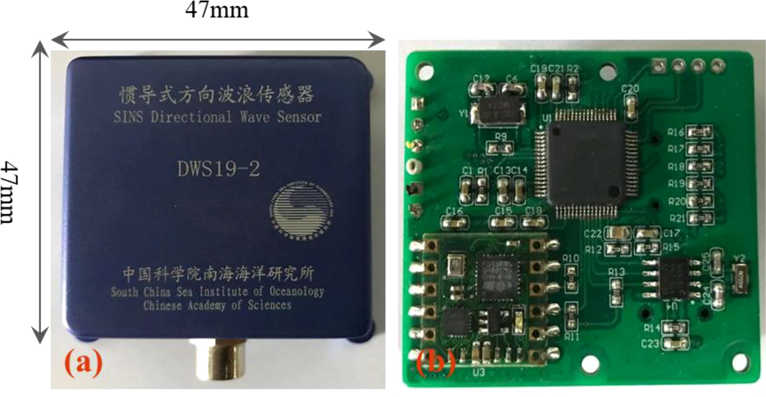
Figure 1 DWS19-2 directional wave sensor: (A) physical picture; (B) signal processing board.

TABLE 1

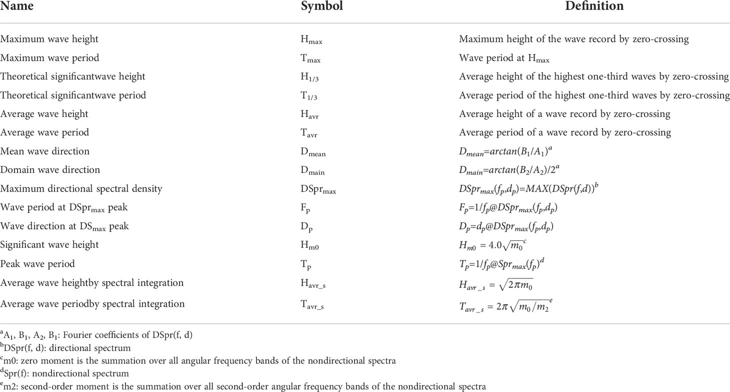
Table 1 Definition of the wave parameters.

FIGURE 2

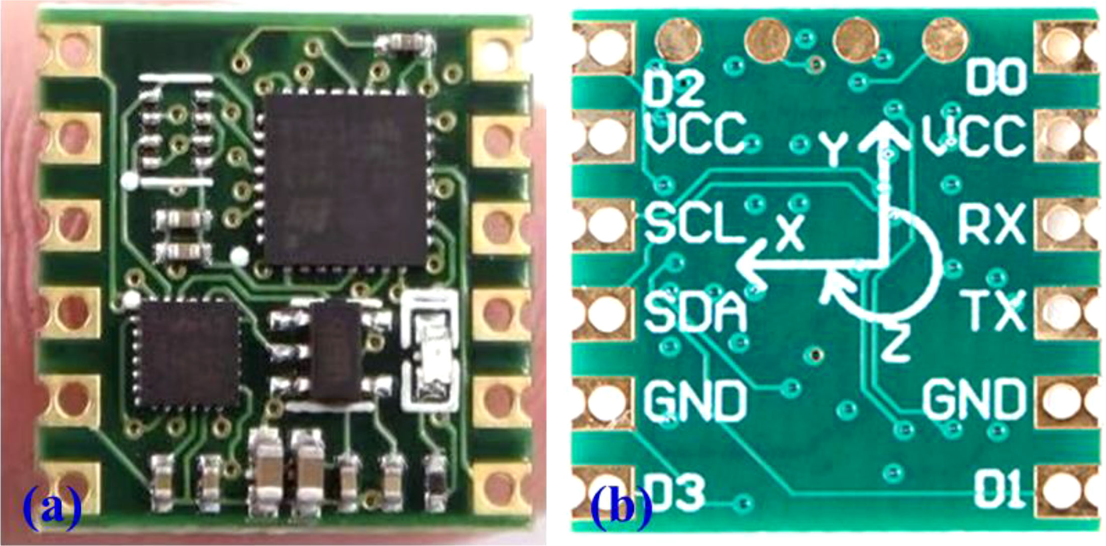
Figure 2 QZ901 IINM: (A) front side; (B) back side.

The high-performance embedded processing chip, namely, STM32F446, was adopted to meet the stringent requirements of the calculations on real-time coordinate projection and fast Fourier transform (FFT), among others. The chip has a 4-channel USART interface, a 3-channel SPI interface, a 2-channel inter integrated circuit (IIC) interface, and two secure digital input/output (SDIO) interfaces. Functions from the official digital signal processing (DSP) library can be invoked to rapidly finish the FFT calculation during wave signal processing. Conducting FFT for 2,048 sets of acceleration data takes no more than 10 ms, a speed that satisfies the demands of real-time wave calculation. The circuit schematic diagram of DWS19-2 wave sensor is shown in Figure 3. The algorithm process of a DWS19-2 measurement consists of the following steps shown as Figure 4. First, the software and hardware are initialized after the sensor had been powered on, and then 2 s later, the 9-axis data are sampled at a frequency of 4 Hz; moreover, the coordinate projection is conducted in every 9-axis data sample. When the sample number reaches 2048, in succession, the wave calculation procedure starts to conduct the frequency-domain numerical integration, the time-based wave parameter statistical analysis, the frequency-based parameter calculation, and the estimation of directional wave spectra. Each sample’s raw data, such as the acceleration of the body coordinate system (BCS), the attitude information (pitch, roll, heading), and the acceleration of the geographic coordinate system (GCS), are recorded in the SD card. It takes approximately 8 min and 50 s to output the wave parameters through the RS232 interface after the sensor is powered up. The reported wave parameters is as follows:

FIGURE 3

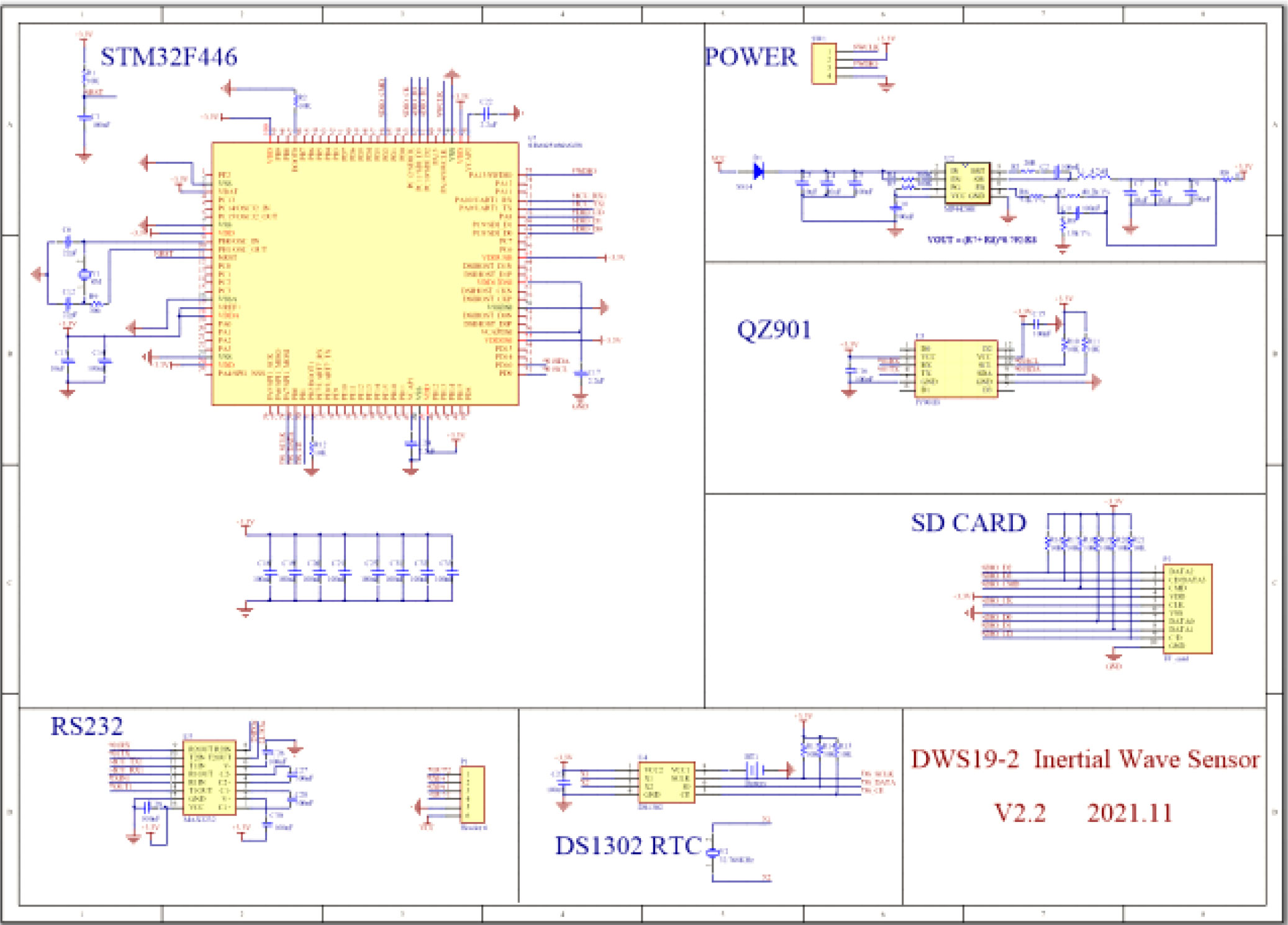
Figure 3 Circuit schematic diagram of DWS19-2 wave sensor.

FIGURE 4

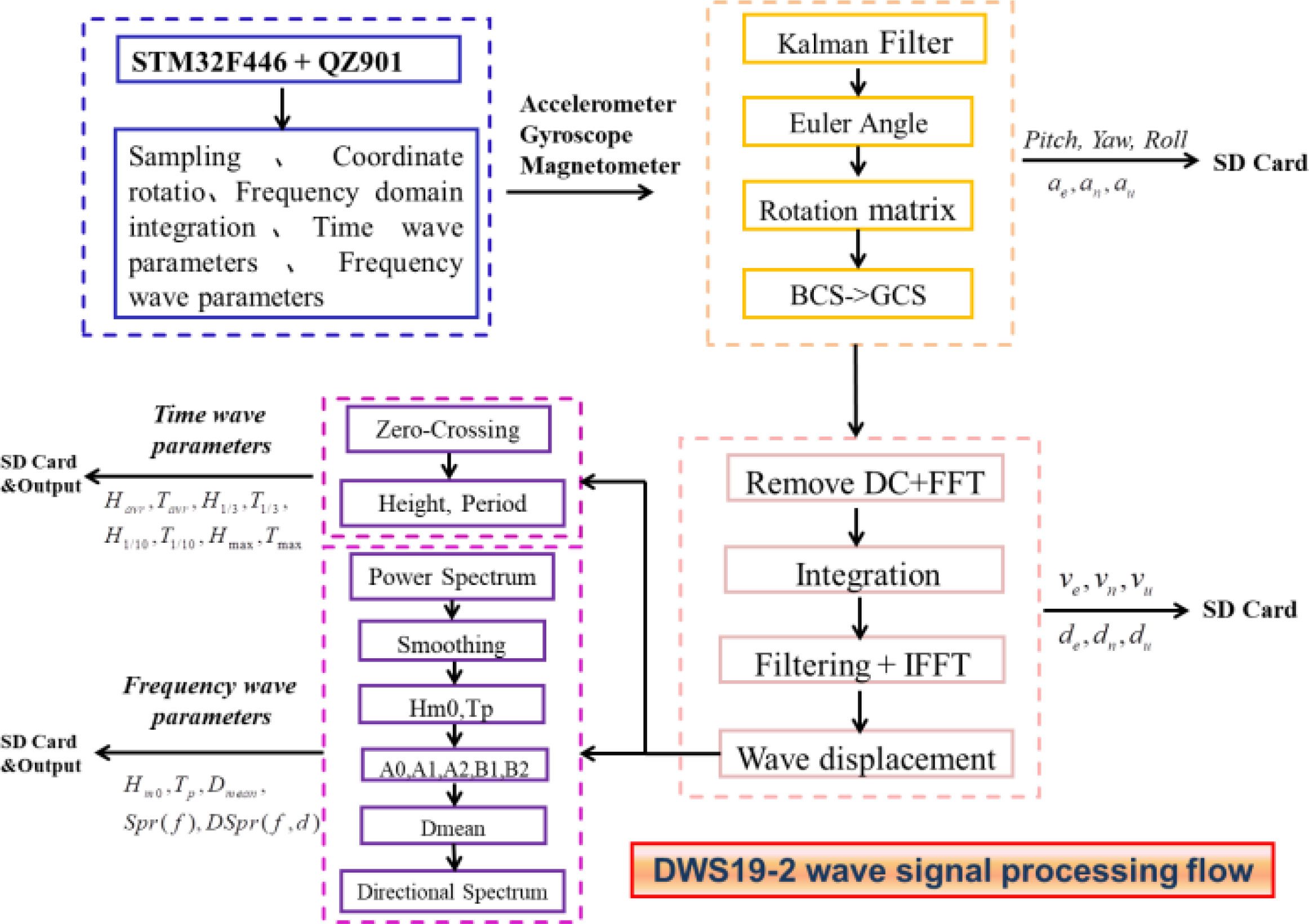
Figure 4 DWS19-2 wave signal processing flow.

$wave, yyyymmddhhmmss,<H_max> <T_max> <H_1/3> <T_1/3> <H_avr> <T_avr> <D_mean> <D_main> <DSpr_max> <F_p> <D_p> <H_{avr_s}> <T_{avr_s}> <cr> <if>

The definitions of each wave parameter are given in Table 1.

On board signal processing

Coordinate projection

Because buoys fluctuate and swing with waves, whether the inertial sensing components of the sensor can remain horizontally stable in a dynamic wave environment directly affects the precision of the wave measurement (Fong et al., 2008; Marin-Perianu et al., 2008). The vertical accelerometer is used to calculate the wave height of the sensor. Because the wave sensor floats continuously changing attitude, coordinate projection is a necessary step to compute the real vertical acceleration relative to the Earth plane. In DWS19-2, the 3-axis accelerations of the BCS can be projected to the GCS by the coordinate projection matrix, the coordinate projection matrix realizing the function of the “digital stabilization platform”.

The coordinate rotation matrix $(C_b^n)$ is calculated by the 3-axis attitude angle,

$$\begin{array}{l}{C}_b^n=C(\psi )C(\theta )C(\varphi )\\ =\left[\begin{array}{lll}\cos (\psi )\hfill & \sin (\psi )\hfill & 0\hfill \\ -\sin (\psi )\hfill & \cos (\psi )\hfill & 0\hfill \\ 0\hfill & 0\hfill & 1\hfill \end{array}\right]\left[\begin{array}{lll}\cos (\theta )\hfill & 0\hfill & \sin (\theta )\hfill \\ 0\hfill & 1\hfill & 0\hfill \\ -\sin (\theta )\hfill & 0\hfill & \cos (\theta )\hfill \end{array}\right]\left[\begin{array}{lll}1\hfill & 0\hfill & 0\hfill \\ 0\hfill & \cos (\varphi )\hfill & -\sin (\varphi )\hfill \\ 0\hfill & \sin (\varphi )\hfill & \cos (\theta )\hfill \end{array}\right]\end{array}$$

where ψ, Φ, and θ stand for the roll, pitch, and heading, respectively. The 3-axis accelerations of the BCS are projected to the GCS via the formula $a_n=a_b{C}_b^n$.

In Figure 3, the Z-axis acceleration is sampled by DWS19-2 in a 0.9 m diameter circular buoy in the offshore sea area of Jiangmen City, Guangdong province. The sampling number is 2048 and the sampling frequency is 4Hz, and the Z-axis acceleration (A_Z) between the BCS and the GCS is compared. The Z-axis acceleration and the calculated displacement (D_Z) after the coordinate projection differ prominently from the BCS values, where the average displacement error reaches 15% (Figure 5).

FIGURE 5

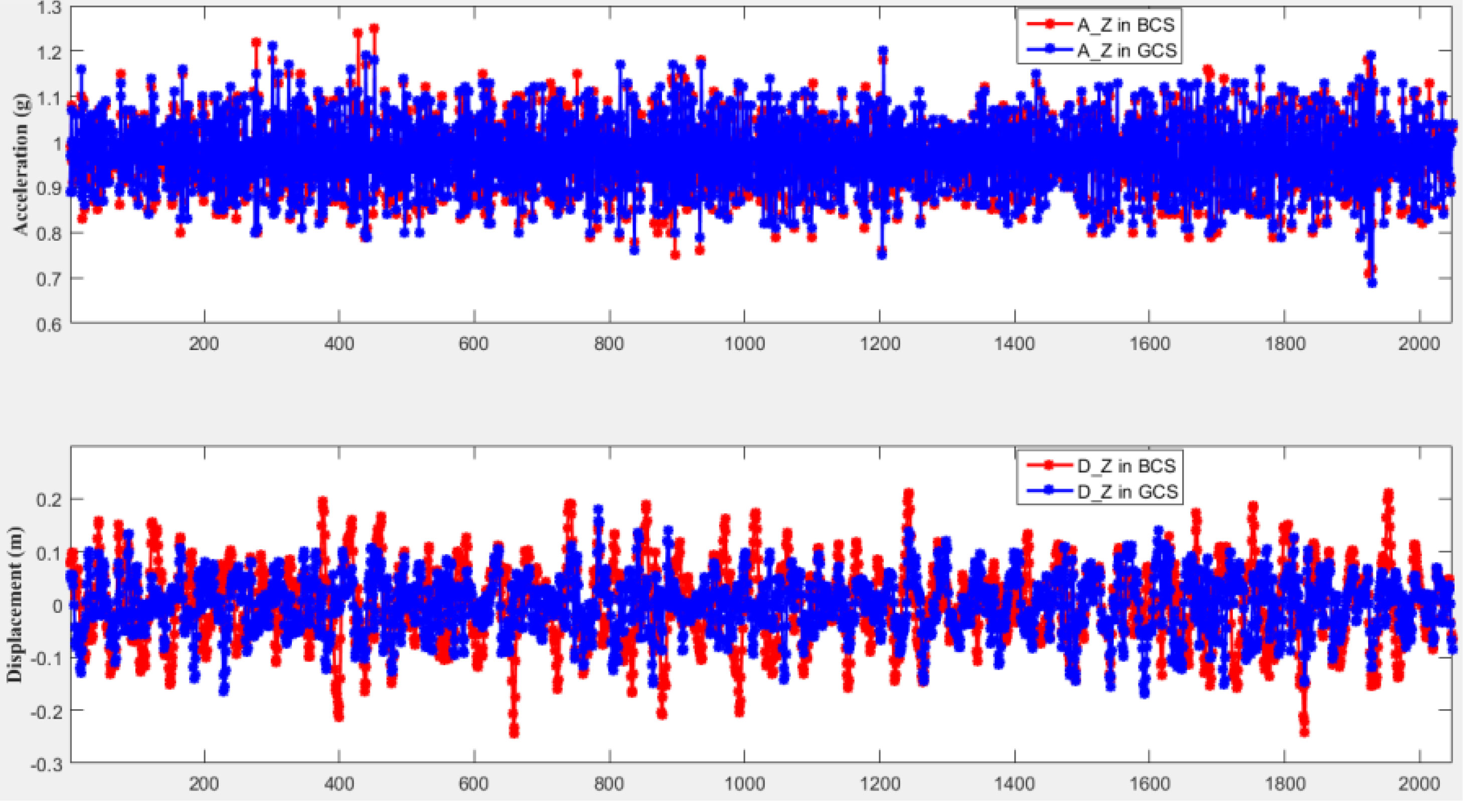
Figure 5 Comparison of accelerations and displacements before and after coordinate projection.

Numerical integration of acceleration

The goal of this part is to develop a reliable process from which the wave displacement signal can be derived from the measured acceleration data via a double integration process. Integration errors must be minimized so that the calculated displacement is very close to the actual displacement.

To date, three integration techniques have been used to determine displacement by measured acceleration: analog integration, time-domain numerical integration, and frequency-domain numerical integration (Lee and Lee, 1996; Pang and Liu, 2001). In principle, the process of double integration can be done electronically with an RC amplification circuit (Ribeiro et al., 1999). Because the circuit components are set at the very beginning of the design, the filter performance of the integration circuit is fixed. For the random wave that occurred in the ocean, the hardware integration does not have filter self-adaptability. Therefore, the analog double integrator is reliable only to measure sinusoidal steady-state displacements. In addition, an unbounded displacement drift can arise after two integrations in the time domain caused by a small DC bias in the acceleration signals. Consequently, an empirical digital filter should be designed to extract the real displacement signal (Rong et al., 2000). By filtering after integration, drift errors are eliminated.

Frequency-domain integration applies the FFT to acceleration first, converting the time-domain acceleration signal to the frequency domain. The inverse FFT (IFFT) is conducted to change the integrated results to time-domain displacement signals. In contrast to the time-domain numerical integration, the frequency-domain integration can effectively restrict the cumulative amplification effect of the low-frequency DC error signals after two integrations, thereby obtaining a more precise and reliable displacement result. As the calculation ability of the high-performance ARM/DSP chip is greatly improved, FFT and IFFT calculations in an embedded chip are feasible. DWS19-2 adopts the frequency-domain numerical integration method, and the calculation process is shown below. In accordance with Formula (1), the FFT is carried out on projected Z-axis accelerations a_n to achieve the real and imaginary components.

$\begin{array}{ll}A(k)={\displaystyle \sum _{n=0}^{N-1}{a}_n{e}^{-j2\pi k\frac{n}{N}}},k=0,\mathrm{1,...,}N-1& (1)\end{array}$

According to the integral transformation properties of the FFT, the displacements are calculated by Formula (2), followed by bandpass filtering of 0.04-0.67 Hz to the displacement signals. Finally, the time-domain displacement signals are achieved through IFFT.

$\begin{array}{ll}S(n)={\displaystyle \sum _{k=0}^{N-1}\frac{1}{-{(2\pi k\Delta f)}^2}}H(k)a_n{e}^{-j2\pi k\frac{n}{N}}& (2)\end{array}$

where $H(k)=\{1,f_d\le kf\le f_{u}0$; Δf stands for the frequency resolution; and f_u and f_d represent the upper and lower cutoff frequencies of the bandpass filter, respectively, which are set as 0.67 (corresponding to 1.5 s) and 0.04 (corresponding to 25 s), respectively, in this paper.

From Figure 6, a series of projected Z-axis accelerations are integrated by two methods in the time domain and frequency domain to obtain the two displacement series. The displacement result of the time-domain displacement displays notable drifting, and an empirical signal filter processing method is needed later to extract the real displacement signals. Although there is phase shift in the FDI, the obvious drift error does not exist in the results of the frequency-domain integration. This phase shift only affects the real-time wave displacement series by FDI, but has no effect on the time wave parameters statistics by the zero-crossing method and the frequency wave parameters by spectral integration method.

FIGURE 6

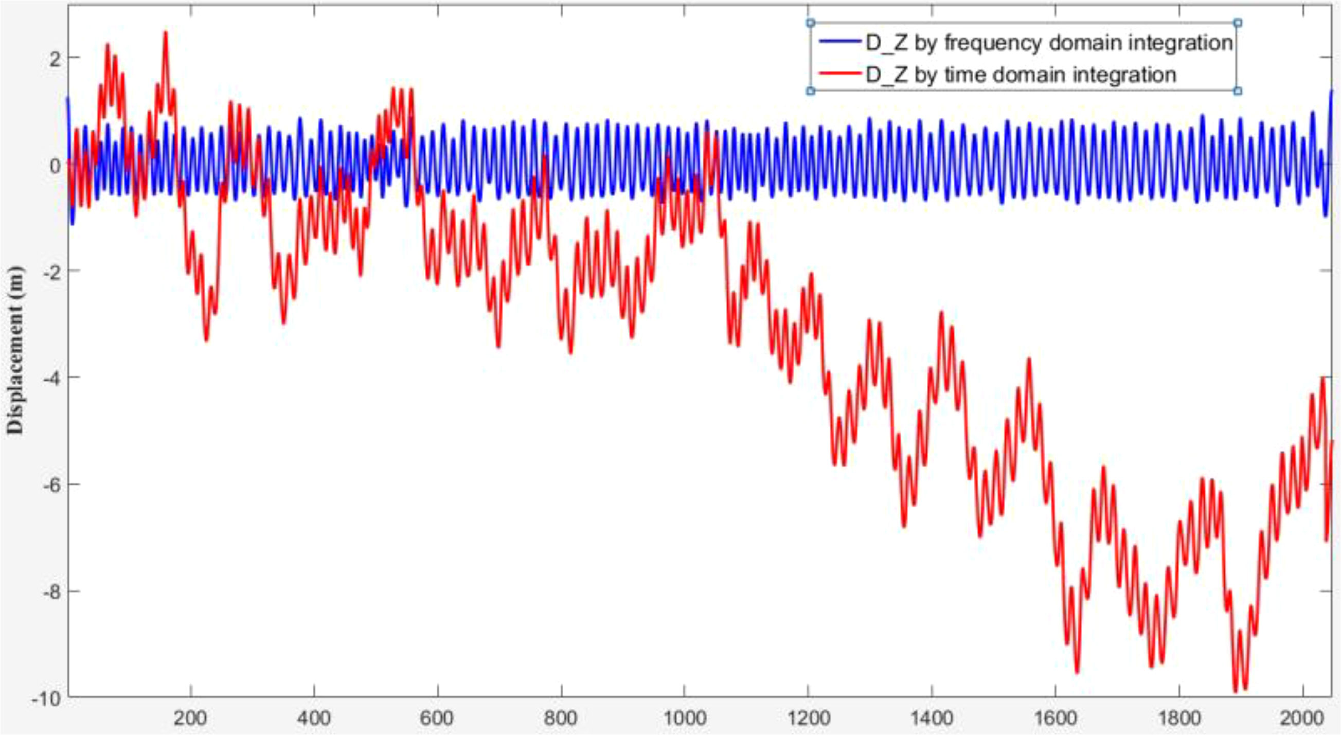
Figure 6 Comparison of displacement obtained by time and frequency domain integration.

Time wave parameters

The DWS19-2 wave sensor’s onboard program contains two methods for calculating wave parameters, the zero-crossing method (Figure 7) and the energy spectrum method, and the corresponding calculation results are time wave parameters and frequency wave parameters, respectively.

FIGURE 7

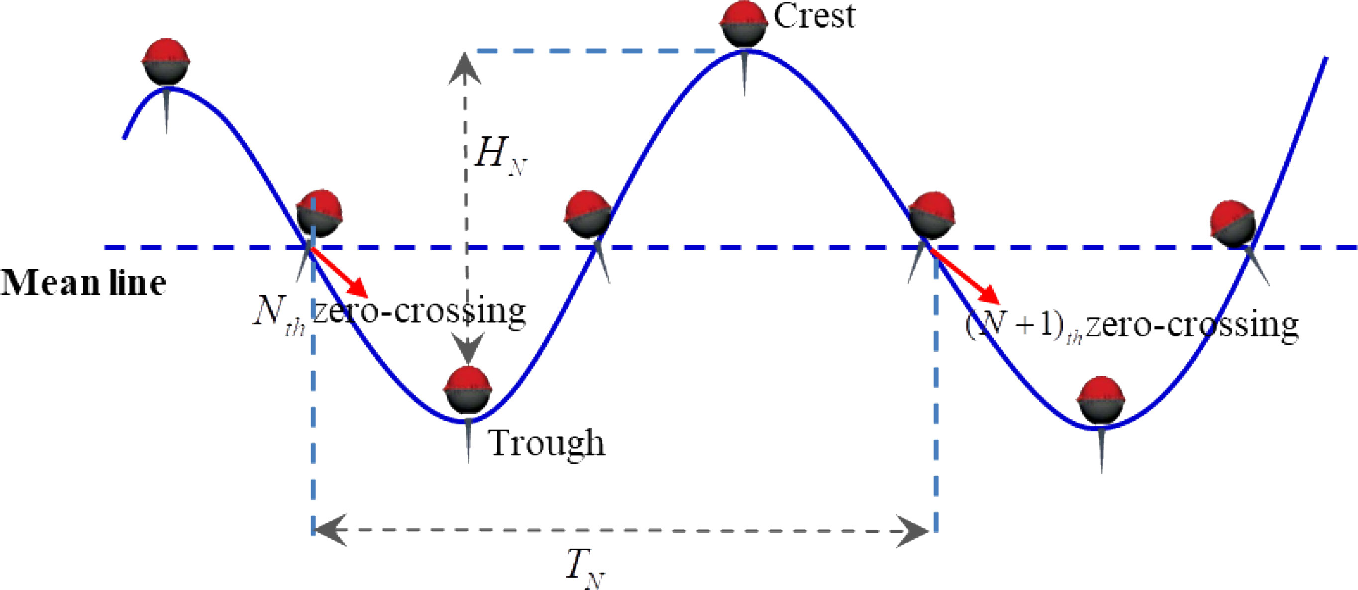
Figure 7 Downward zero-crossing method.

For a wave displacement series, the zero-crossing method can be used to conduct wave characteristic statistics. The first step is to determine the average value for the reference zero line and take the first intersection between the downward movement position of the buoy and the zero line as a zero-crossing starting point. Then, the next crossing point is searched as the second zero-crossing end point. The time difference and the vertical displacement difference between the two downward zero-crossing points are the observed wave period and wave height, respectively. Subsequently, all the observed wave heights and wave periods are ranked in descending order to obtain statistical wave parameters, including H_max, T_max, H_1/3, T_1/3, H_1/10, T_1/10, H_avr, and T_avr.

Frequency wave parameters

The power spectrum method can be used to obtain the frequency wave parameters. The non-directional power spectrum can be calculated as follows:

$\begin{array}{ll}Spr(w_k)=\frac{\Delta t}{2\pi N}|A_k{|}^2,w_k=k\Delta w,k=0,1,\mathrm{2,...}N/2& (3)\end{array}$

where A_k is the FFT of the displacement time series S(n). The power spectrum is further smoothed according to the following equation:

$\begin{array}{ll}\overline{Spr(w_k)}=\frac{1}{4}Spr(w_{k-1})+\frac{1}{2}Spr(w_k)+\frac{1}{4}Spr(w_{k+1})& (4)\end{array}$

Then, the wave spectral momentums are calculated. The calculation equations for the zero-order momentum m₀ and the second-order momentum m₂ are as follows:

$\begin{array}{ll}{m}_0=\left[\frac{1}{2}Spr(w_0)+{\displaystyle \sum _{k=1}^{N/2-1}Spr(w_k)+\frac{1}{2}Spr(w_{N/2})}\right]\Delta w& (5)\end{array}$

$\begin{array}{ll}{m}_2=\left[\frac{1}{2}Spr(w_0)w_0^2+{\displaystyle \sum _{k=1}^{N/2-1}Spr(w_k)w_K^2+\frac{1}{2}Spr(w_{N/2})w_{N/2}^2}\right]\Delta w& (6)\end{array}$

Then, the frequency wave parameters, including H_{avr_s}, T_{avr_s}, H_m0, and Tp, are calculated according to the equations defined in Table 1.

A four-day observed wave height time series from a mooring buoy in the Indian Ocean in 2021 is shown in Figure 8. The time parameters (H_avr, H_1/3) obtained by the zero-crossing method are highly consistent with the frequency wave parameters (H_{avr_s}, H_m0) obtained by the power spectra method. The average error between H_avr and H_{avr_s} is 0.02 m. The H_m0 is approximately 8% higher than H_1/3. Reasons for the deviation between the time and frequency parameters were explained by Longuet-Higgins (1952). An assumption for approximating significant wave height by H_m0 is that wave spectra are narrow banded. In Longuet-Higgins (1980), the finite spectral width is the likely explanation for the differences between H_1/3 and H_m0, with H_m0 values typically being approximately 5 to 10 percent greater than H_1/3 values, which is consistent with the studies in this paper.

FIGURE 8

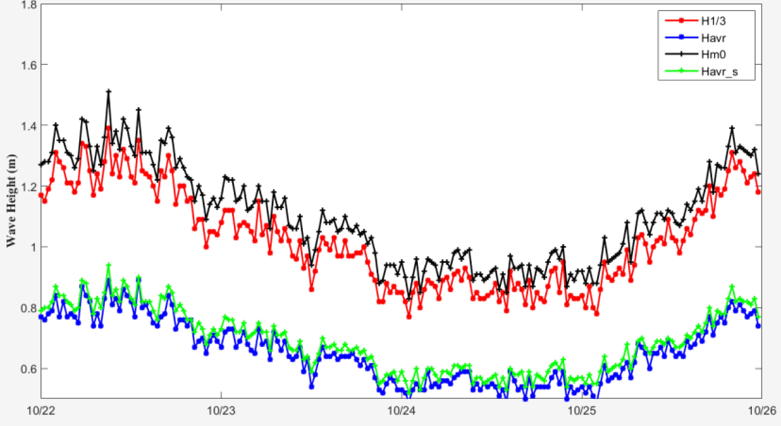
Figure 8 Comparison of time and frequency wave height.

Directional wave spectrum

The directional wave spectrum DSpr(f, θ) is the energy spectrum reflecting the internal directional structure of the wave and represents the energy distribution of wave components in different directions with respect to the frequency.

Directional wave spectra provide the distribution of wave elevation variance as a function of both wave frequency (f) and wave direction (θ). A directional wave spectrum can be written as

$\begin{array}{ll}DSpr(f,\theta )=\frac{A_0}{2}+{\displaystyle \sum _{n=1}^2[A_{n}cos(n\theta )+B_n\sin (n\theta )]}& (7)\end{array}$

The first five Fourier coefficients A₀, A₁, A₂, B₁, B₂ are given by $A_0=\frac{C_{11}}{\pi },A_1\frac{Q_{12}}{k\pi },B_1=\frac{Q_{13}}{k\pi },A_2=\frac{C_{22}-C_{33}}{k^2\pi },B_2=\frac{2C_{23}}{k^2\pi }$

D_mean and D_main are calculated by

$\begin{array}{ll}{D}_{mean}=\arctan \left(\frac{B_1}{A_1}\right),D_{main}=\frac{1}{2}\arctan \left(\frac{B_2}{A_2}\right)& (8)\end{array}$

DWS19-2 measures buoy heave, pitch, roll, and heading, and the subscripts of Q_xy and C_xy are defined as follows:

1 = displacement along the Z-axis, which corresponds to buoy heave after coordinate projection, which can be obtained by integrating the acceleration twice in the frequency domain.

2 = wave slope along east–west, which corresponds to buoy tilt in this direction.

3 = wave slope along south-north, which corresponds to buoy tilt in this direction

For each measured data point by DWS19-2, heading is used to convert pitch and roll to wave slopes along the east–west and south–north directions, respectively.

Here, C_xy is the cospectrum, and Q_xy is the quadrature spectrum, which can be given by

$\begin{array}{ll}{C}_{xy}=(Re[X]*Re[Y]+Im[X]*Im[Y])/N& (9)\end{array}$

$\begin{array}{ll}{Q}_{xy}=(\mathrm{Im}[X]*Re[Y]-Im[X]*Im[Y])/N& (10)\end{array}$

where X and Y are frequency domain representations of the time series x and y, respectively.

DWS19-2 can report power spectra by query command “?MNMD<\r>“ after every wave measurement (2048 data4Hz). The output format of directional spectrum is

$TSPMA, yyyymmddhhmmss,<FreNum>,<FreStart>,<df>,<FreEnd>

<Fre_1>,<1*5>,<DirSpec>

…

<Fre_1>,<72*5>,<DirSpec>

<Fre_2>,<1*5>,<DirSpec>

…

<Fre_2>,<72*5>,<DirSpec>

…

<Fre_100>,<1*5>,<DirSpec>

…

<Fre_100>,<72*5>,<DirSpec>

DWS19-2 outputs 7,200 directional spectrum values, which are obtained by 100 frequency intervals multiplied by 72 direction intervals. FreNum is defined as 100, FreStart is the starting frequency defined as 0.041 Hz, df refers to the frequency interval of 0.006 Hz, and FreEnd represents the cutoff frequency of 0.627 Hz.

Laboratory and filed testing

Laboratory turntable testing

A buoy floating in a wave is generally assumed to motion in a circular orbit, in which the buoy itself maintains an approximately upright position in the sea without rotating (Dean and Dalrymple, 1991; Boccotti, 2000). To evaluate the measurement validity of wave sensors from different manufacturers, a mechanical wave motion simulation laboratory was established in the National Center of Ocean Standards and Metrology (NCOSM). A circular motion turntable with an adjustable period and height is the key simulation device, which is very similar to the ferris wheel in an amusement park. The turntable wave simulator (TWS) is shown in Figure 9. From April 21–23, 2021, three wave height simulation tests were conducted on DWS19-2 at 1 m, 3 m and 6 m on the TWS. With each simulated wave height, seven different periods of measurement were carried out. The average wave height (H_avr) and wave period (T_avr) output by DWS19-2 obtained by zero-crossing were compared with the standard height and periods, respectively.

FIGURE 9

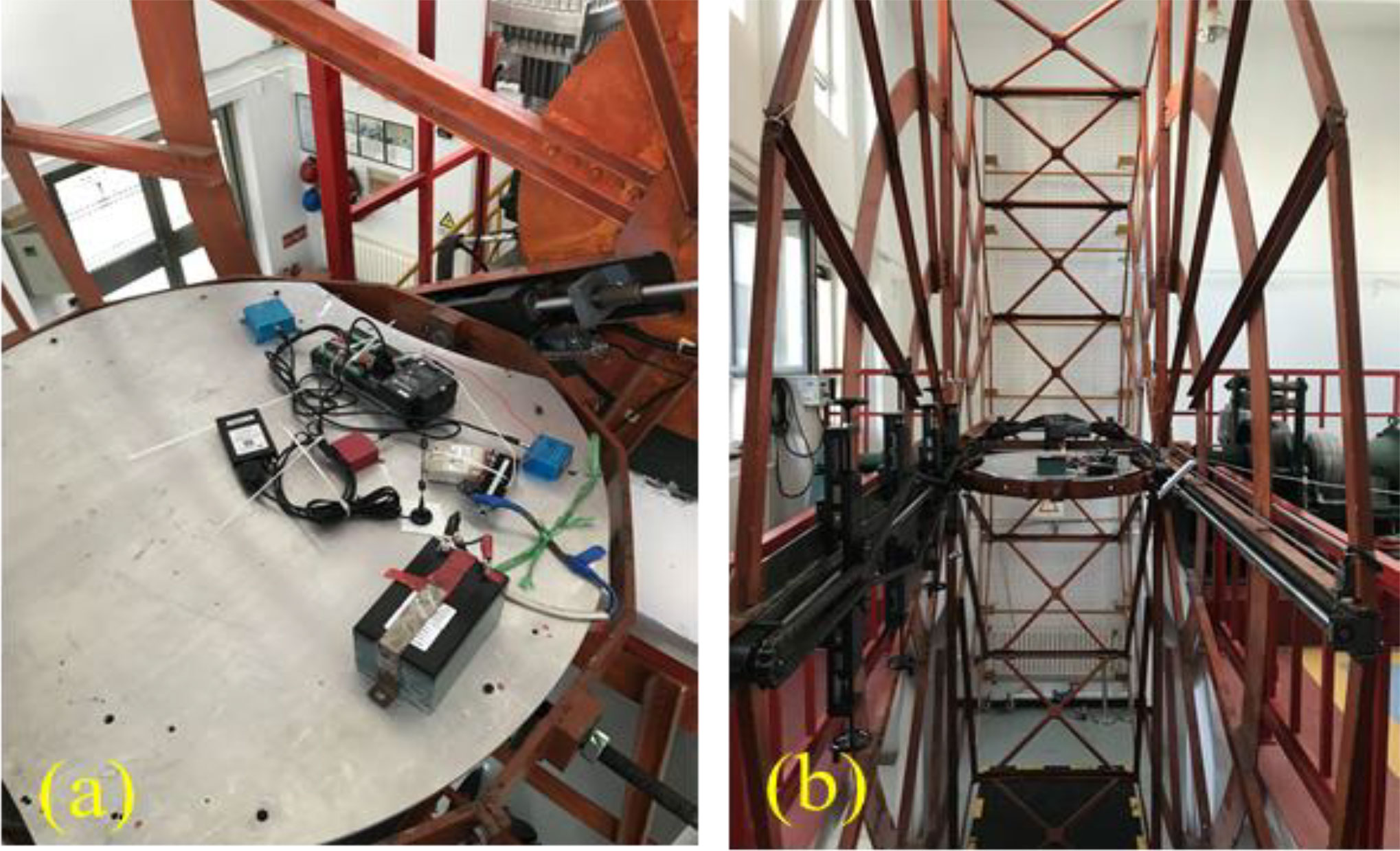
Figure 9 Wave simulation turnable: (A) Installation of DWS19-2 and data acquisition system (B) Turntable simulator device.

At a height of 1 m, simulation measurements were conducted in seven periods of 25.0 s, 17.6 s, 10.3 s, 8.3 s, 6.4 s, 4.7 s, and 3.7 s. At a height of 3 m, simulation measurements were conducted in seven periods of 14.2 s, 9.9 s, 7.6 s, 6.2 s, 5.2 s, and 4.5 s. At a height of 6 m, simulation measurements were conducted in seven periods of 25.0 s, 16.8 s, 12.7 s, 10.2 s, 8.5 s, 7.3 s, and 6.4 s. The test results are listed in Tables 2–4.

TABLE 2

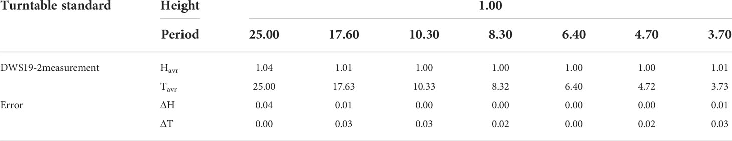
Table 2 Measurement at a height of 1 m (height unit: m; period unit: s).

TABLE 3

Table 3 Measurement at a height of 3 m (height unit: m; period unit: s).

TABLE 4

Table 4 Measurement at a height of 6 m (height unit: m; period unit: s).

Overall, for DWS19-2, at a height of 1 m, the errors in height measurement were within 1% (except for the measurement at 25.00 s), and those for period measurement were within 0.05 s. At heights of 3 m and 6 m, the errors in height measurement were within ±2%. Those in the period measurement were basically within 0.06 s (except for 14.2 s at 3 m and 16.8 s at 6 m).

Field comparison

For the purpose of filed comparison, a DWS19-2 was mounted on a spherical wave buoy deployed in Haimen Bay (22.93° N, 116.52°E) in the Northern South China Sea, hereinafter referred to as DWS19 Wave Buoy. The diameter of the wave buoy was 0.9m, powered by solar energy. The collected wave data was transmitted back to shore based data center in every half hour by 4G (fourth generation) link. The water depth of the buoy site is about 15 m. There is a gravity-acceleration-type DWR-MKIII Waverider buoy was deployed by the South China Sea Branch of the State Oceanic Administration, the straight-line distance between the two buoys was about 150m (Figure 10). DWS19 Wave buoy used the same mooring system as DWR-MKIII, which was composed of a buoyancy ball, an elastic cable, a nylon rope, and a grip anchor. The control cabin had a serious leakage ten days later because of a water tightness issue, so comparison test was only carried out from 11 January to 21 January 2022 for about 10 days with a wave measurement interval of 30 min. A total of 473 simultaneous wave data were collected by two buoys. The significant wave height H_m0, the peak wave period T_p and the mean wave direction D_mean were used for the comparison purposes.

FIGURE 10

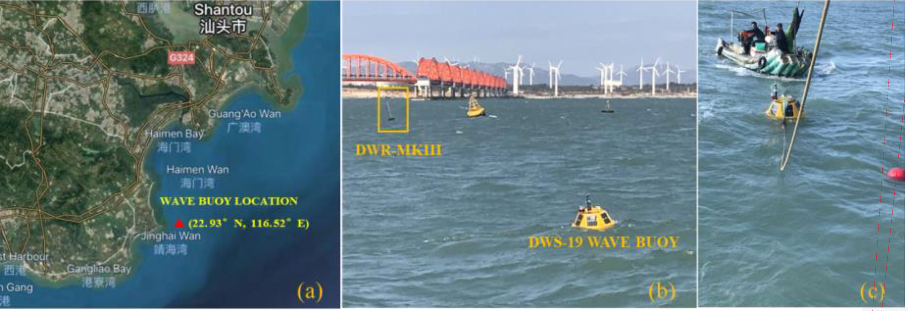
Figure 10 Filed comparison with DWR-MKIII wave buoy: (A) Filed comparison location. (B) Offshore comparison site. (C) Deployment of DWS19 Wave Buoy.

A time series and scatter plots of H_m0, T_p, D_mean were shown in Figures 11 and 12. Statistics of mean deviation and standard deviation of each parameter are shown in the Table 5. The wave height of DWR-MKIII Waverider is about 5% higher than DWS19 wave buoy, this bias may be due to that the DWR-MKIII Waverider has a better wave tracking performance iin short waves.We have analyzed the hydrodynamic response of the DWS19 buoy using ANSYS AQWA software (Version 18.2) prior to the deployment. The response amplitude operator of heave can reach 1 only when the incident wave period is greater than 3 s, which means the current designed DWS19 wave buoy is not ideal for short-wave (<3 s) measurement. The user manual of DWR-MKIII indicates that waves with a period of 1.5-30 s can be measured, so it is better than DWS19 buoy in short wave component measurement. Therefore, the wave height measurement of DWS19 may be slightly smaller than that of DWR-MKIII because the contribution of short waves is excluded. A review of the period series shows that the overall trend is almost the same as the wave height, the overall mean deviation between DWS19 buoy and DWR-MKIII is 0.07s. The wave period increases or decrease with the wave height. Therefore, we can conclude that this sea area is dominated by wind wave during the comparison period. For the direction series reveals that the overall trend of DWS19 is in overall agreement with the DWR-MKIII with a mean deviation of 2°and standard deviation of 10°, the wave is coming from the southwest. But during low wave height period, especially when the wave height is less than 1m, relatively larger direction differences are observed. We speculated that when the wave height is small, the DWS19 buoy with large mass has poor wave tracking performance, the pitch, roll and heavy of the buoy are correspondingly small. Therefore, the accuracy of wave direction calculated by these three parameters is poor during small wave height period.

FIGURE 11

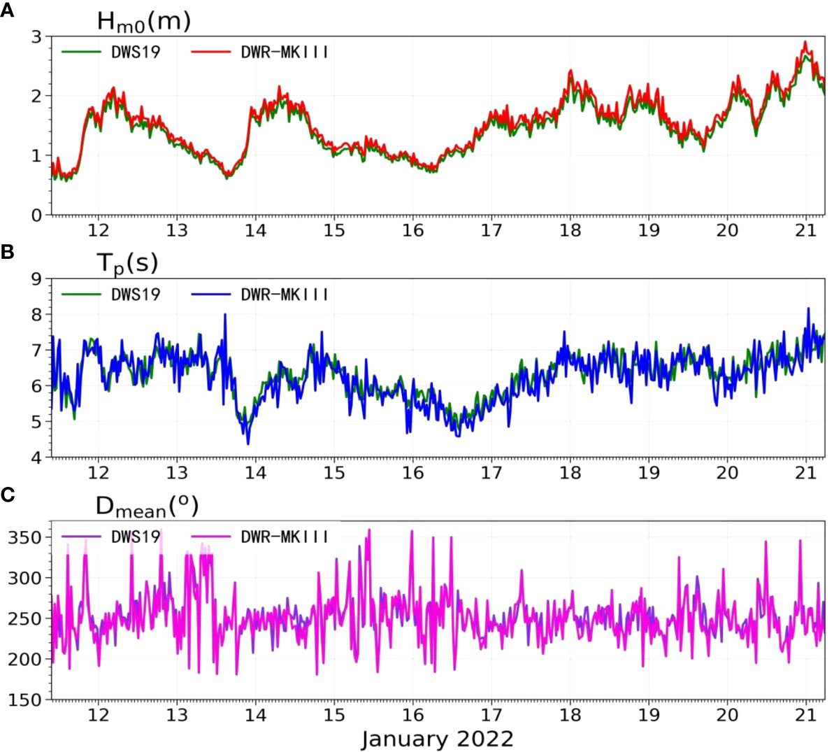
Figure 11 Time series of H_m0, T_p, D_mean observed by DWS19 buoy and DWR-MKIII.

FIGURE 12

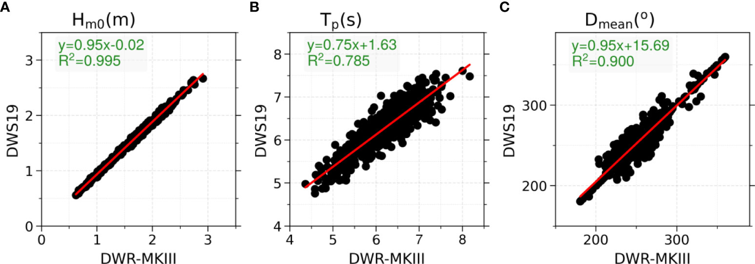
Figure 12 Scatter plots of H_m0, T_p, D_mean observed by DWS19 buoy and DWR-MKIII.

TABLE 5

Table 5 Statistics of mean deviation(MD) and standard deviation(SD).

Applications

Wave observation in the equatorial Indian Ocean

On October 16, 2020, researchers from the SCSIO deployed an air-sea coupling observation buoy (ASCOB_EIO) in the equatorial Indian Ocean (79.0°E, 2.0°N) at a depth of 4,100 m. The buoy was 3 m in diameter and equipped with a DWS19-2 wave sensor with a wave observation interval of 30 min. The real-time data were transmitted to the data center of the SCSIO with the Iridium and Bei Dou satellite communication link. By May 30, 2021, a total of 10,848 wave data sets, including wave height, period, and wave direction, had been obtained. The time series of H_1/3, H_m0, H_avr, T_1/3, T_avr, and D_mean from ASCOB_EIO are given in Figure 13.

FIGURE 13

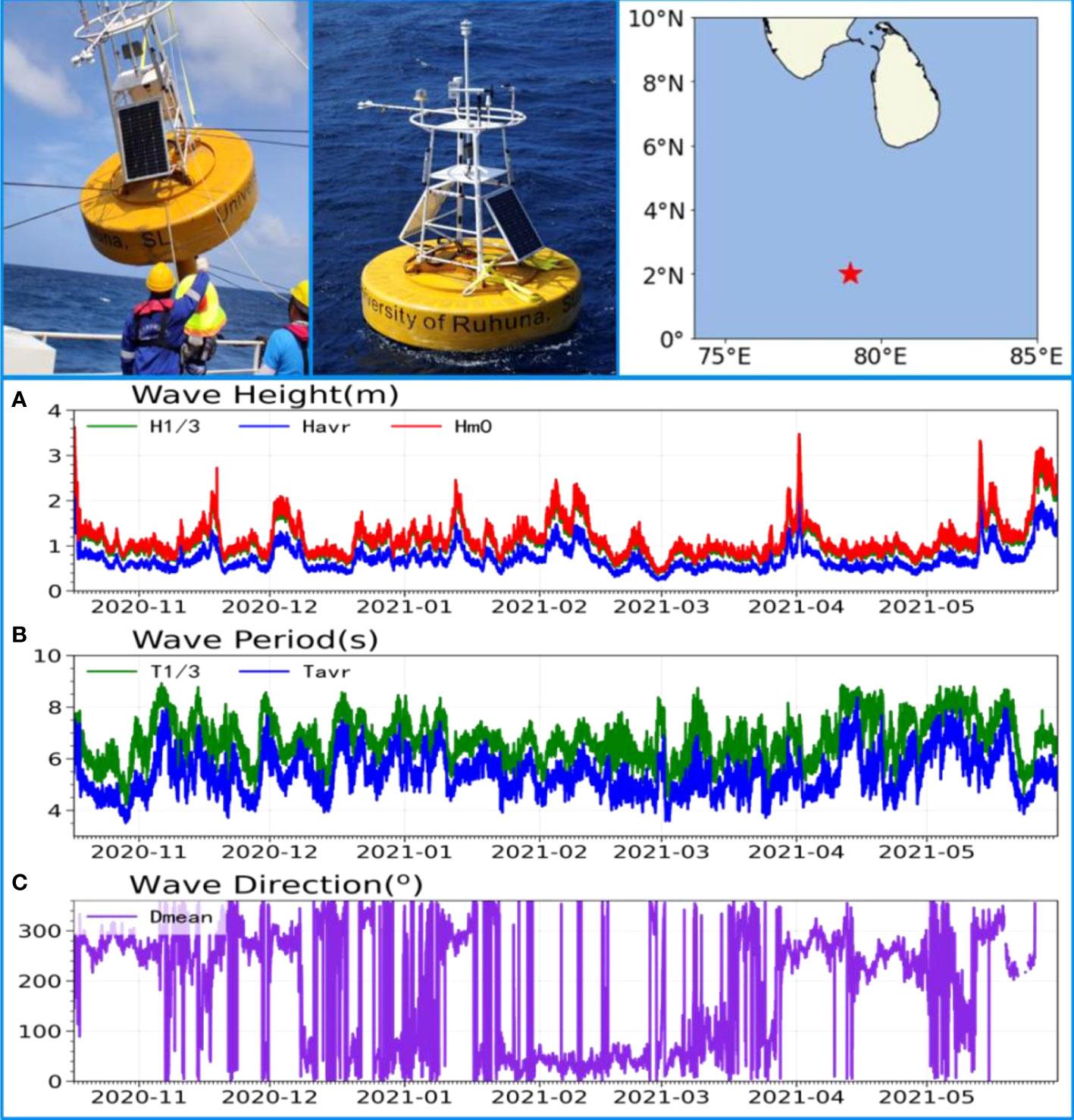
Figure 13 Wave observation in the Equatorial Indian Ocean.

Wave observation in the South China Sea

On July 6, 2021, a 3 m diameter marine environment monitoring buoy (MEMB_ZH) was deployed by researchers from Sun Yat-sen University (SYU) at a water depth of 12 m in coastal Zhuhai (113.20°E, 21.55°N). The buoy transmits real-time data back to the SYU shore-based data center by a 4G link. The buoy was equipped with DWS19-2, with a wave sampling interval of 30 min. Notably, data were missing for approximately 5 days, from August 7 to 12, because of the failure of buoy control sysytem. By October 8, 2021, 3,710 wave data sets, including wave height, period, and wave direction, had been obtained. The time series of H_1/3, H_m0, H_avr, T_1/3, T_avr, and D_mean from MEMB_ZH are given in Figure 14.

FIGURE 14

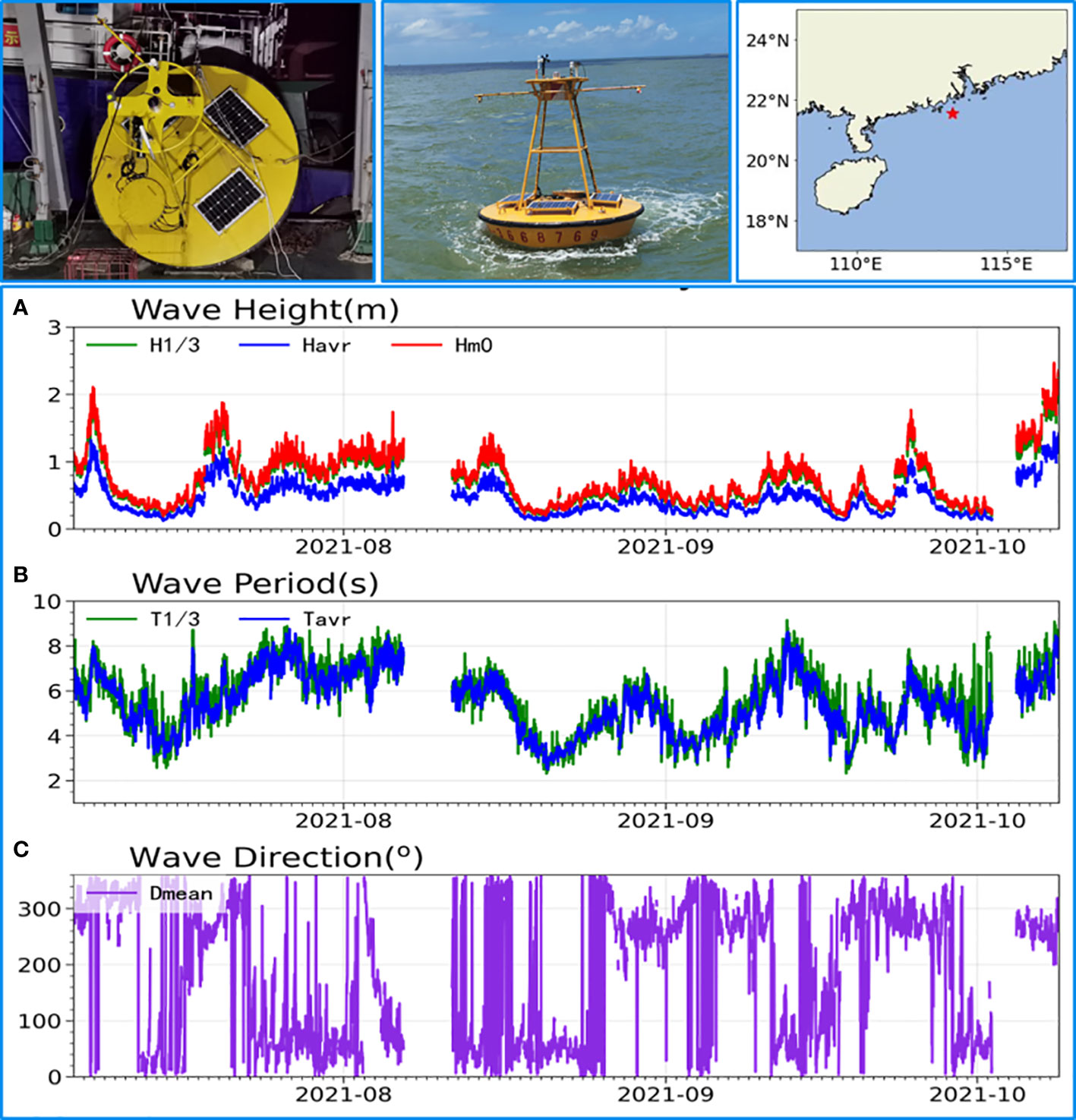
Figure 14 Wave observation in Zhuhai.

On June 23, 2021, 1.5 m diameter ocean dynamic observation buoys (ODOB_ZJ) were deployed by Guangdong Ocean University (GOU) at a depth of 10 m in coastal Zhanjiang (109.0°E, 20.0°N). The buoy was equipped with DWS19-2 and transmits real-time data to the GOU shore-based data center. The wave sampling interval was 10 min. By November 8, 2021, a total of 20,016 wave data sets, including wave height, period, and wave direction, had been obtained. The time series of H_1/3, H_m0, H_avr, T_1/3, T_avr, and D_mean from ODOB_ZJ are given in Figure 15.

FIGURE 15

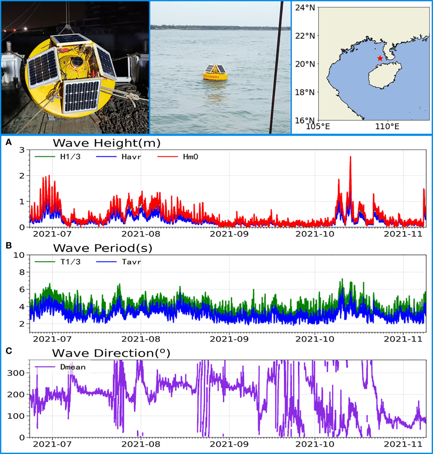
Figure 15 Wave observation in Zhanjiang.

On September 22, 2021, a 0.6 m diameter surface drifter equipped with DWS19-2 was dropped by researchers from the SCSIO at a depth of 3,700 m in the northern South China Sea (115.08°E, 17.34°N). The wave sampling interval was 1 h. The real-time data were sent back to the SCSIO data center by the Bei Dou communication link. By November 9, the buoy had drifted to coastal southern Vietnam, and a total of 925 wave data sets had been collected. The time series of H_1/3, H_m0, H_avr, T_1/3, T_avr, and D_mean are given in Figure 16. Notably, data were missing for approximately 3 days, from October 16 to 19, because of the failure of the satellite communication link. At 11:00 a.m. on October 16, the drifter was located in the influence wind circle of the Kompasu typhoon, and the 6.94 m significant wave height was measured.

FIGURE 16

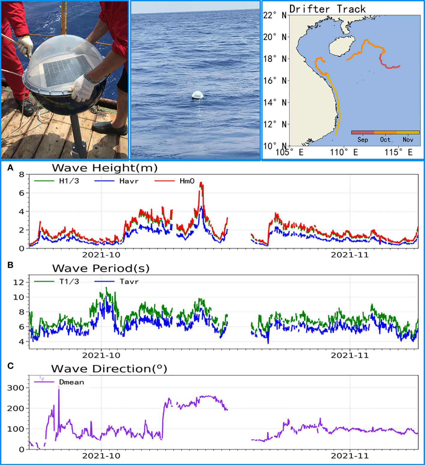
Figure 16 Wave observation by a drifter in the South China Sea.

Conclusions

DWS19-2 is a small-sized inertial wave sensor with low power consumption developed by SCSIO, CAS. The onboard data processing algorithms include coordinate projection, acceleration-displacement numerical integration, time wave parameters by the zero-crossing method, frequency wave parameters by the power spectrum method, and the estimation of the directional wave spectrum. Seven different periods of testing at heights of 1 m, 3 m, and 6 m were performed on the wave simulation turntable of NCOSM. In addition, the on-site comparison with the wave rider DWR-MKIII buoy was also completed at the beginning of 2022. Based on the results of the turntable test and filed comparison, DWS19-2 featured high measurement accuracy, a small size, low power consumption, and reliability in marine environments. It offered an innovative method for wave measurement in some mobile and portable applications. Following are the author’s conclusions:

1. Digital stabilization technology was applied for real-time coordinate projection, thus eliminating the dependence on mechanical/electrical stabilization mechanisms. DWS19-2 is small in size and easy to install, which could effectively increase the measurement accuracy in dynamic wave environments.

2. In terms of acceleration-displacement integration, compared with time-domain numerical integration, frequency-domain integration performed better in suppressing the integral drifting errors caused by DC acceleration deviation.

3. The significant wave height obtained by the power spectrum method was 5% to 8% larger than that obtained by the zero-crossing method, which is also consistent with previous research.

4. According to the wave simulation test on the standard turntable, high measurement accuracy of the wave height (< ± 2%) and wave period (< ± 0.05 s) was obtained by DWS19-2, reaching the excellent measurement index level. The results of filed comparison with DWR-MKIII wave buoy show that the mean deviation of H_m0 and T_p are -0.09m and 0.07s respectively. The mean deviation and standard deviation of wave direction is 2.08° and 10.21° respectively.

5. Wave observations from anchored buoys in the Equatorial Indian Ocean, coastal Zhuhai, coastal Zhanjiang, and drifters in the South China Sea revealed that DWS19-2 is suitable for various types of marine platforms with stable and reliable performance in harsh marine environments.

Data availability statement

All the data used in the article can be obtained by email to emhvdWZoQHNjc2lvLmFjLmNu. We will also post all the data in this paper on the data center website of SCSIO (South China Sea Institute of Oceanology, Chinese Academy of Sciences, http://data.scsio.ac.cn/).

Author contributions

Conceptualization: FZ. Methodology: FZ and SZ. Hardware design: FZ. Algorithm design and simulation: FZ and RZ. Software coding: FZ and RZ. Turntable test: SZ. Filed comparison: FZ, SZ and RZ. Writing-review and editing: FZ, SZ and RZ. Project administration: FZ. Funding acquisition: FZ. All authors have read and agreed to the published version of the manuscript. All authors contributed to the article and approved the submitted version.

Funding

This work is supported by the National Natural Science Foundation of China (42176189, 41706102), Scientific Instrument Development Project, Chinese Academy of Sciences (YJKYYQ20180063), Young S&T Talent Training Program of Guangdong Provincial Association for S&T, China (SKXRC202220), Youth Innovation Promotion Association CAS (2020341) and the development fund of South China Sea Institute of Oceanology of the Chinese Academy of Sciences (SCSI0202204).

Acknowledgments

The authors extend their appreciation to the crews of R/Vs “Shiyan 3” for assistance with buoy deployment. The electrical design, system integration and signal processing algorithm were supported by Dr. Zhanlin Liang. To make the best use of buoy wave data, researchers can apply data access under the supervision of the Natural Science Foundation of China after the priority period.

Conflict of interest

The authors declare that the research was conducted in the absence of any commercial or financial relationships that could be construed as a potential conflict of interest.

Publisher’s note

All claims expressed in this article are solely those of the authors and do not necessarily represent those of their affiliated organizations, or those of the publisher, the editors and the reviewers. Any product that may be evaluated in this article, or claim that may be made by its manufacturer, is not guaranteed or endorsed by the publisher.

References

Boccotti P. (2000). Wave mechanics for ocean engineering (Amsterdam; New York: Elsevier Science).

Google Scholar

Datawell B. V. Home of the waverider. Available at: http://www.datawell.nl/ (Accessed 29 Novermber 2021).

Google Scholar

Dean R. G., Dalrymple R. A. (1991). Water wave mechanics for engineers and scientists (Singapore: World Scientific).

Google Scholar

Doong D. J., Lee B. C., Kao C. C. (2011). Wave measurements using GPS velocity signals. Sensors. (Basel). 11, 1043–1058. doi: 10.3390/s110101043

PubMed Abstract | CrossRef Full Text | Google Scholar

Fong W. T., Ong S. K., Nee A. Y. C. (2008). Methods for in-field user calibration of an inertial measurement unit without external equipment. Meas. Sci. Technol. 19, 85202. doi: 10.1088/0957-0233/19/8/085202

CrossRef Full Text | Google Scholar

Lee S. G., Lee M. T. (1996). Integration of measured acceleration to determine the vibration characteristics of bridges. Comput. Struct. Eng. 9, 107–115.

Google Scholar

Longuet-Higgins M. S. (1952). On the statisticaldistribution of the height of sea waves. J. Mar. Res. 11, 245–266.

Google Scholar

Longuet-Higgins M. S. (1980). On the distribution of the heights of sea waves: Some effects of nonlinearity and finite band width. J. Geophys. Res. Oceans. 85, 1519–1523. doi: 10.1029/JC085iC03p01519

CrossRef Full Text | Google Scholar

Longuet-Higgins M. S. (1985). Accelerations in steep gravity waves. J. Phys. Oceanogr. 15, 1570–1579. doi: 10.1175/1520-0485(1985)015<1570:AISGW>2.0.CO;2

CrossRef Full Text | Google Scholar

Marin-Perianu M., Chatterjea S., Marin-Perianu R., Bosch S., Dulman S., Kininmonth S., et al. (2008). “Wave monitoring with wireless sensor networks,” in 2008 international conference on intelligent sensors, sensor networks and information processing (Sydney, NSW, Australia: IEEE), 611–616.

Google Scholar

Pang G., Liu H. (2001). Evaluation of a low-cost MEMS accelerometer for distance measurement. J. Intell. Robot. Syst. 30, 249–265. doi: 10.1023/A:1008113324758

CrossRef Full Text | Google Scholar

Qi Z., Li S., Li M., Dang C., Sun D., Zhang D., et al. (2019). Research on the algorithm model for measuring ocean waves based on satellite GPS signals in China. Sensors. (Basel). 19, 541. doi: 10.3390/s19030541

CrossRef Full Text | Google Scholar

Ribeiro J. G. T., Freire J. L. F., Castro J. T. P. (1999). Some comments on digital integration to measure displacements using accelerometers. Shock Vib. Dig. 32, 52.

Google Scholar

Rong T., Shen C., Yuan Z., Xu S. (2000). Principle of measureing the displacement with accelerometer and the error analysis. Huazhong. Ligong. Daxue. Xuebao/J. Huazhong. (Cent. China). 28, 58–60.

Google Scholar

TRIAXYS Directional wave buoy. Available at: https://axystech.wpengine.com/?page_id=5314/ (Accessed 22 Novermber 2021).

Google Scholar