Air-water CO2 and water-sediment O2 exchanges over a tidal flat in Tokyo Bay

Despite the potential for carbon storage in tidal flats, little is known about the details of relevant processes because of the complexity of intertidal physical and chemical environments and the uniqueness of the biota. We measured air-water carbon dioxide (CO₂) fluxes and water-sediment oxygen (O₂) fluxes over a tidal flat in Tokyo Bay by the eddy covariance method, which has the potential to facilitate long-term, broad-scale, continuous monitoring of carbon flows in tidal flats. The results indicated that throughout the tidal flat in Tokyo Bay, CO₂ was taken up from the atmosphere at a rate of 6.05 ± 7.14 (mean ± SD) mmol m⁻² hour⁻¹, and O₂ was taken up from the water into the sediment at a rate of 0.62 ± 1.14 (mean ± SD) mmol m⁻² hour⁻¹. The fact that the CO₂ uptake rate was about 18 times faster than the previously reported average uptake rate in the whole area of Tokyo Bay was attributable to physical turbulence in the water column caused by bottom friction. Statistical analysis suggested that light intensity and water temperature were the major factors responsible for variations of CO₂ and O₂ exchange, respectively. Other factors such as freshwater inputs, atmospheric stability, and wind speed also affected CO₂ and O₂ exchange. High rates of O₂ uptake from the water into the sediment surface and high rates of atmospheric CO₂ uptake into the water column occurred simultaneously (R² = 0.44 and 0.47 during day and night, respectively). The explanation could be that photosynthetic consumption of CO₂ and production of O₂ in the water column increased the downward CO₂ (air to water) and O₂ (water to sediment) fluxes by increasing the concentration gradients of those gases. Resuspension of sediment in the low-O₂ layer by physical disturbance would also increase the O₂ concentration gradient and the O₂ flux in the water.

Introduction

Coastal marine areas are important sites of carbon storage because photosynthetic rates are high, and sedimentation and burial of carbon sequesters carbon from the atmosphere for long periods of time (Mateo et al., 1997; Mcleod et al., 2011). Quantification of carbon fluxes in coastal waters is therefore critical to identifying effective strategies for mitigating the adverse effects of anthropogenic CO₂ emissions. Recent studies have compared carbon accumulation rates and have concluded that the rates in several coastal areas are ten times larger than the rates in the open ocean (e.g., Nellemann et al., 2009). However, there is a paucity of analyses of atmospheric CO₂ exchange rates in coastal areas compared with the numerous studies of carbon accumulation rates in sediments (Frankignoulle, 1988; Kayanne et al., 1995; Borges et al., 2005; Tokoro et al., 2008; Tokoro et al., 2014). Those studies have indicated that autotrophic production in coastal ecosystems results in net CO₂ absorption from the atmosphere and counteracts the tendency of those ecosystems to emit CO₂ produced by the decomposition of organic matter from land runoff. However, precise estimation of atmospheric CO₂ exchange in coastal areas is challenging because of the complexity of the spatiotemporal variations of coastal CO₂ exchange.

Carbon accumulation rates in tidal flats (10-120 g C m^-2 year^-1 × 0.13 million km², (Widdows et al., 2004; Sanders et al., 2010; Endo and Otani, 2019; Murray et al., 2019) have been estimated to be on the same order of magnitude as the rates associated with other vegetated coastal habitats like salt marshes (151 g C m^-2 year^-1 × 0.4 million km², Nellemann et al., 2009). However, despite numerous measurements, little is known about the details of carbon flows in tidal flats because of the uniqueness of the biota, the complexity of the carbon flows, the intertidal conditions, and inputs of brackish water. Because tidal flats located near human population centers are easily affected by anthropogenic impacts associated with eutrophication, pollution, and land reclamation, analysis of interactions between carbon fluxes and human activities is therefore an urgent issue.

Evaluation of the interactions between atmospheric CO₂ and carbon fluxes in tidal flats is especially difficult. The mechanism of exchange is quite different between periods of sediment submergence (air–water) and exposure (air–sediment). Furthermore, the estimation of air–water CO₂ fluxes using empirical wind-driven equations, which have been used in previous studies of other coastal areas and the ocean, is likely to be inaccurate because air–water CO₂ fluxes are likely to be greatly affected by tidal-driven effects (e.g., O'connor and Dobbins, 1958; Raymond and Cole, 2001; Borges et al., 2004). Therefore, direct measurement techniques have been used to estimate atmospheric CO₂ exchange rates over tidal flats. The chamber method is a direct measurement technique that estimates CO₂ exchanges from changes of CO₂ density inside a chamber on the surface of the water or sediment. The method can be applied to both air–water and air–sediment fluxes in tidal flats (Middelburg et al., 1996; Migné et al., 2002; Spilmont et al., 2005; Klaassen and Spilmont, 2012; Sasaki et al., 2012; Otani and Endo, 2019). However, the temporal duration and spatial range of the chamber method are limited because the measurement area is usually less than 1 m² and the hand-operation is required for each measurement. Therefore, a comprehensive analysis of atmospheric CO₂ exchange over tidal flats is still difficult with the method. The eddy covariance (EC) method is another direct measurement method and is applicable to measurements without submerged/exposed conditions. Although the measurement area depends on several conditions like the fluctuation of wind direction, the CO₂ exchange in a scale of several hundred meters to several kilometers can be measured without any hand-operation. Although use of the EC method is costly because the equipment is expensive and the correction procedure is complex, the EC method has been used in several studies to measure CO₂ fluxes over tidal flats because the fluxes are integrated over large spatiotemporal scales (Zemmelink et al., 2009; Polsenaere et al., 2012).

Water-sediment O₂ exchange is important proxy for the analysis of inorganic and organic carbon dynamics in aquatic ecosystems because O₂ exchange usually relates to CO₂ exchange in the mole ratio of near 1:1 through photosynthetic activities, respiration and organic matter decomposition. Although the measurement of atmospheric O₂ exchange has not been reduced to practice due to the difficulty in the measurement with enough sampling rate, the EC method has been applied for the measurement of water-sediment exchange (Kuwae et al., 2006; Berg et al., 2022). The EC method for O₂ exchange has an advantage of the temporal duration and spatial range as well as for CO₂ exchange. Additionally, the EC method can measure O₂ exchange directly and avoid altering the natural conditions (e.g., flow, light and metabolism) compared with other methods using incubated cores or benthic chambers.

In this study, we used the EC method to measure atmospheric CO₂ exchange over a tidal flat in Tokyo Bay. We used other EC devices to measure exchange of O₂ between the water and sediment for comparison with the CO₂ exchange and determined whether biological activities in the water and sediment were related. Our goal was to identify the factors that regulated those fluxes. Most of the tidal flats in Tokyo Bay have disappeared because of urban development and reclamation of coastal land during the last century, and measurements in the remaining tidal flats were therefore important for the prediction of how future human activities will likely affect conditions in the bay.

Materials and methods

In situ measurements were conducted over the Banzu tidal flat in Tokyo Bay during February 2011. The Banzu tidal flat is an intertidal sand flat with an area of 7.6 km² and a shallow slope of 1/1000 situated on the eastern shore of Tokyo Bay, Japan (Figure 1). The sediments are fine sand flat with a median grain size of 170-190 μm (Uchiyama, 2007). The tidal range during the measurement was 0.7-1 m and about half of the area was submerged at high tide. There are no macrophytes on the tidal flat, and microphytobenthos on the sediment (2200 mg Chl-a m^-3 and 90 mg C m^-2, Hosokawa, 1999) account for most of the primary production. The biomass of the secondary producers was larger than of the primary producers and was reported to be 1500 and 20,000-40,000 mg C m^-2 in September as of bacteria and macrobenthos (mostly bivalves), respectively (Hosokawa, 1999). Although the biomass of macrobenthos in winter was reported to be one-tenth the mass of in summer, the secondary producers in the tidal flat were considered to exceed the primary producers in the biomass through the year. The large biomass of secondary producers indicates a large organic carbon fixation from plankton or detritus inflowed from the surrounding areas like Tokyo Bay. This suggested that estimation of atmospheric CO₂ exchange without direct measurements should be difficult due to large carbon input come from outside the tidal flat. Although the tidal flat consists of an estuarine delta connected to the Obitsu River (watershed area: 273.2 km²), water exchange would be driven mainly by tidal exchange because the flow rate was far smaller than the tidal current and could not be quantified by the former observations (e.g., Uchiyama, 2007). The water of Tokyo Bay has been reported to be an atmospheric CO₂ sink because of the photosynthetic activity of phytoplankton (10-20 mg Chl-a m^-3) which is enhanced by sewage inputs from the surrounding urban area (Kubo et al., 2017; Tokoro et al., 2021).

FIGURE 1

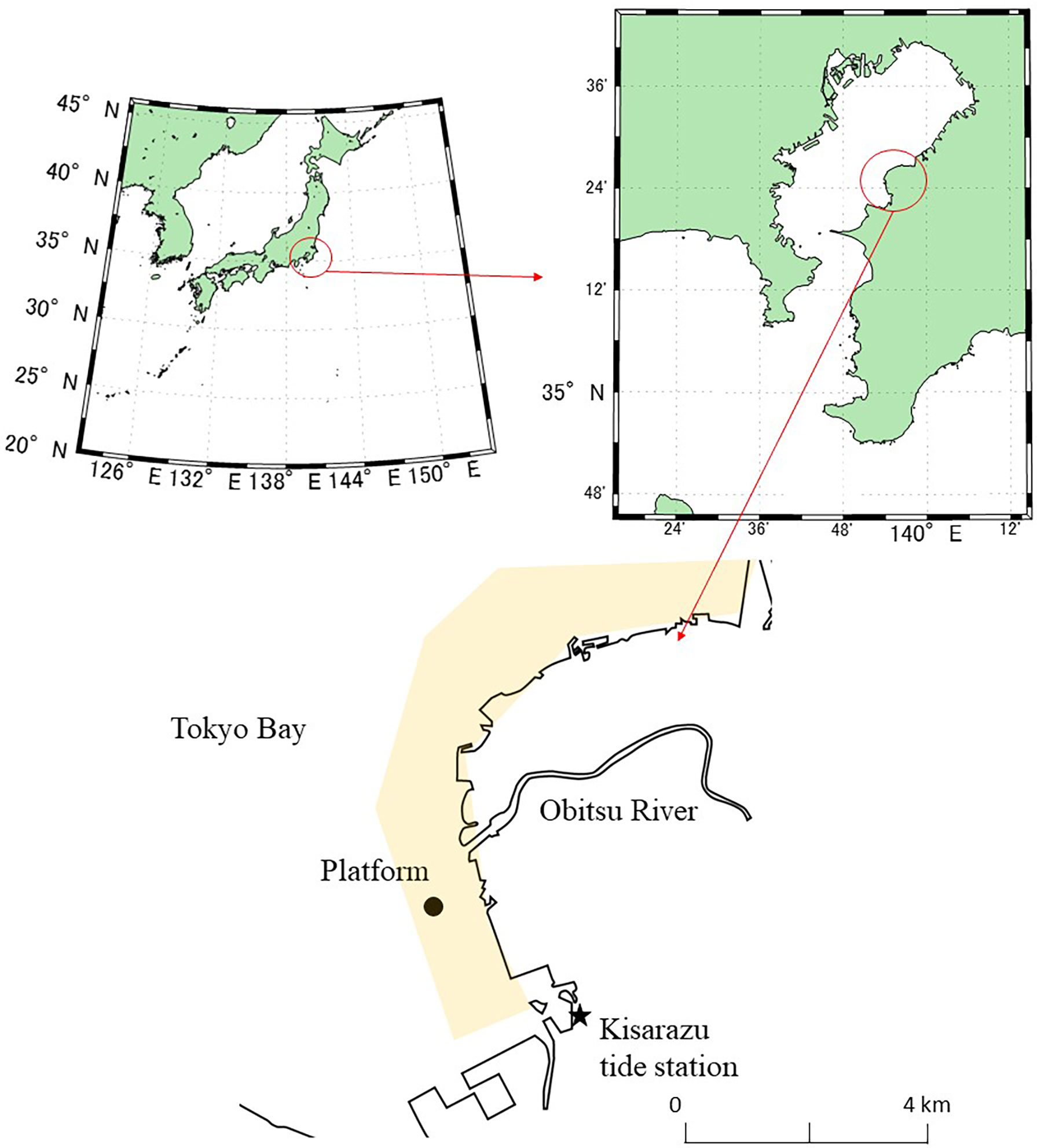
Figure 1 Location of the measurement site (Banzu tidal flat, Tokyo Bay, Japan). The yellow shading indicates the area of the tidal flat during low tide.

The EC method for measuring atmospheric CO₂ exchange determines vertical CO₂ fluxes within the atmosphere by measurements at high frequency (10–20 Hz) of eddy movement vertically and atmospheric CO₂ density. The EC method can estimate atmospheric CO₂ exchange from measurements in air at an altitude of more than several meters and is thus applicable to measurements in the intertidal zone. The EC method also enables continuous and automatic measurements to be made over broad spatiotemporal scales. Comprehensive analysis is thus easier with the EC method than with other onsite measurement methods. We used the following equation to calculate CO₂ exchange (F; positive and negative values mean atmospheric CO₂ efflux and influx from/to water or sediment, respectively) every 30 minutes:

$\begin{array}{ll}F=\overline{{\rho }_c\text{'}w\text{'}}·F_1+\mu \frac{{\rho }_c}{{\rho }_d}\overline{{\rho }_v^{\text{'}}{w}^{\prime }}·F_2+{\rho }_c(1+\mu \frac{{\rho }_v}{{\rho }_d})\frac{\overline{T_a\text{'}w\text{'}}}{T_a}·F_2& (1)\end{array}$

where F₁ and F₂ are the transfer coefficients that correct the frequency attenuation of the CO₂ exchange for the response time of the sensor, path-length averaging, sensor separation, signal processing, and the averaging time of each measurement (Massman, 2000). The first term on the right-hand side of Eq. 1 is the product of F₁ and the uncorrected CO₂ exchange calculated as the covariance of the CO₂ density ρ_c and vertical wind speed w (the bar and prime symbols indicate the mean and the deviation from the mean, respectively). The wind speed was corrected using a double rotation to make the average vertical wind speed zero during the 30-min time interval (Lee et al., 2004). The second and third terms are the product of F₂ and the Webb–Pearman–Leuning correction for the fluxes of latent heat and sensible heat, respectively (Webb et al., 1980). These terms correct for the change of air volume due to changes of moisture and temperature, respectively. The other symbols in Eq. 1 are as follows: ρ_d, dry air density; ρ_v, water vapor density; T_a, air temperature; and μ, ratio of molar weight of dry air to water vapor.

Although the EC method facilitates coastal measurements, the estimated fluxes have been associated with large uncertainties, especially for air–water CO₂ fluxes (Vesala et al., 2012; Blomquist et al., 2014; Kondo et al., 2014; Tokoro et al., 2014; Ikawa and Oechel, 2015). Several studies reported that these uncertainties were caused by the spatiotemporal heterogeneities of water temperature or turbulence conditions (Rutgersson and Smedman, 2010; Mørk et al., 2014). Although several studies have suggested methods to correct air–water CO₂ fluxes estimated by the EC method (Prytherch et al., 2010; Edson et al., 2011; Landwehr et al., 2014; Tokoro and Kuwae, 2018), we made the following simple corrections during the post-processing procedure because the measurement in this study included air–sediment CO₂ fluxes that were not covered by the above correction methods.

We used two operations to detrend measurement parameters and exclude CO₂-exchange outliers in this study. Detrending is a necessary procedure in the EC method because long-term variations that are unrelated to CO₂ eddy movement must be removed. The three main types of detrending methods involve use of mean values, linear approximation, and high-pass (recursive) filtering. The appropriate method depends on the complexity of the long-term trend. In this study, we used high-pass filtering because the temporal changes in the tidal flat were complex. High-pass filtering was carried out with an exponential moving average as follows:

$$x_i=\alpha ·x_{i-1}+\left(1-\alpha \right)·y_i (2)$$

where x_i and y_i are the filtered and original datum at time t_i. α is the time constant of the filtering and was set to 1.7×10⁻³ seconds in accord with McMillen (1988). We used the median absolute deviation (MAD) of the CO₂ exchange as a criterion for excluding outliers (Rousseeuw and Croux, 1993).

$$MAD=median\left\{\right|X_i-median(X)\left|\right\} (3)$$

where X_i is the original datum. A scaled MAD (=1.4826×MAD) was used as an alternative to the standard deviation as an outlier criterion to avoid an outlier effect on the mean and standard deviation. This criterion was suitable for the outlier exclusion of EC data because the outlier criterion was an order of magnitude larger than the average value. In this study, a CO₂ exchange rate that deviated from the median of all the CO₂ exchange data by more than three times the scaled MAD was identified as an outlier and was excluded.

The EC method for O₂ exchange between the water and sediment was basically the same as the EC method for CO₂ exchange. The O₂ exchange was determined from the covariance of O₂ and the vertical current velocity because the change of water volume with temperature and moisture could be ignored. A sampling rate somewhat more than several Hz would be enough for O₂ and current velocity measurements because the water eddy transport at a frequency of 0.3–1.4 Hz would be the main contribution to O₂ exchange according to previous studies (Kuwae et al., 2006; Berg et al., 2022). In addition, the transfer coefficients (F₁ and F₂ in Eq. 1) could be ignored because any related parameter such as the path-length averaging distance and sensor separation are far smaller for O₂ EC devices than for CO₂ EC devices. The time lag between the O₂ and current measurement should be corrected because the time response of O₂ is slower than that of other devices like the current velocimeter. The details of the time lag correction have been described by Kuwae et al. (2006). The post-processing procedure of detrending and outlier exclusion were applied using the linear approximation and the scaled MAD, respectively, because the long-term changes of O₂ were less complicated than those of atmospheric CO₂.

CO₂ EC data were recorded every 30 minutes from 17 February 2011 at 11:30 to 24 February 2011 at 22:00. The EC measurement devices for CO₂ were installed on a platform on the tidal flat (35.401°C N, 139.893°C E) where the water depth was about 0.3–1.0 m at high tide during the measurement period (Figure 2). The platform was located near the edge of the tidal flat, and the altitude of the platform was almost zero. The duration of the exposure period was about 11–13 hours during the measurement. We used an open-path CO₂ analyzer (LI-7500; LI-COR) and a 3-D sonic anemometer (CSAT-3, Campbell) for the EC measurement of atmospheric CO₂ density and atmospheric eddy diffusion, including air temperature, respectively. The devices were placed at the top of the platform (about 5 m from the bottom). All EC data were measured at a sampling rate of 20 Hz, and the atmospheric CO₂ exchange was calculated every 30 minutes. The footprint, which is an index of measurement range of the EC measurement, depends on the measurement height, wind speed, atmospheric stability, and the roughness of the measurement site (here, 0.005 m was assumed to be the roughness of the tidal flat). Footprint estimation (Kljun et al., 2004) indicated that 90% of the CO₂ exchange measurement came from< 270 m upwind.

FIGURE 2

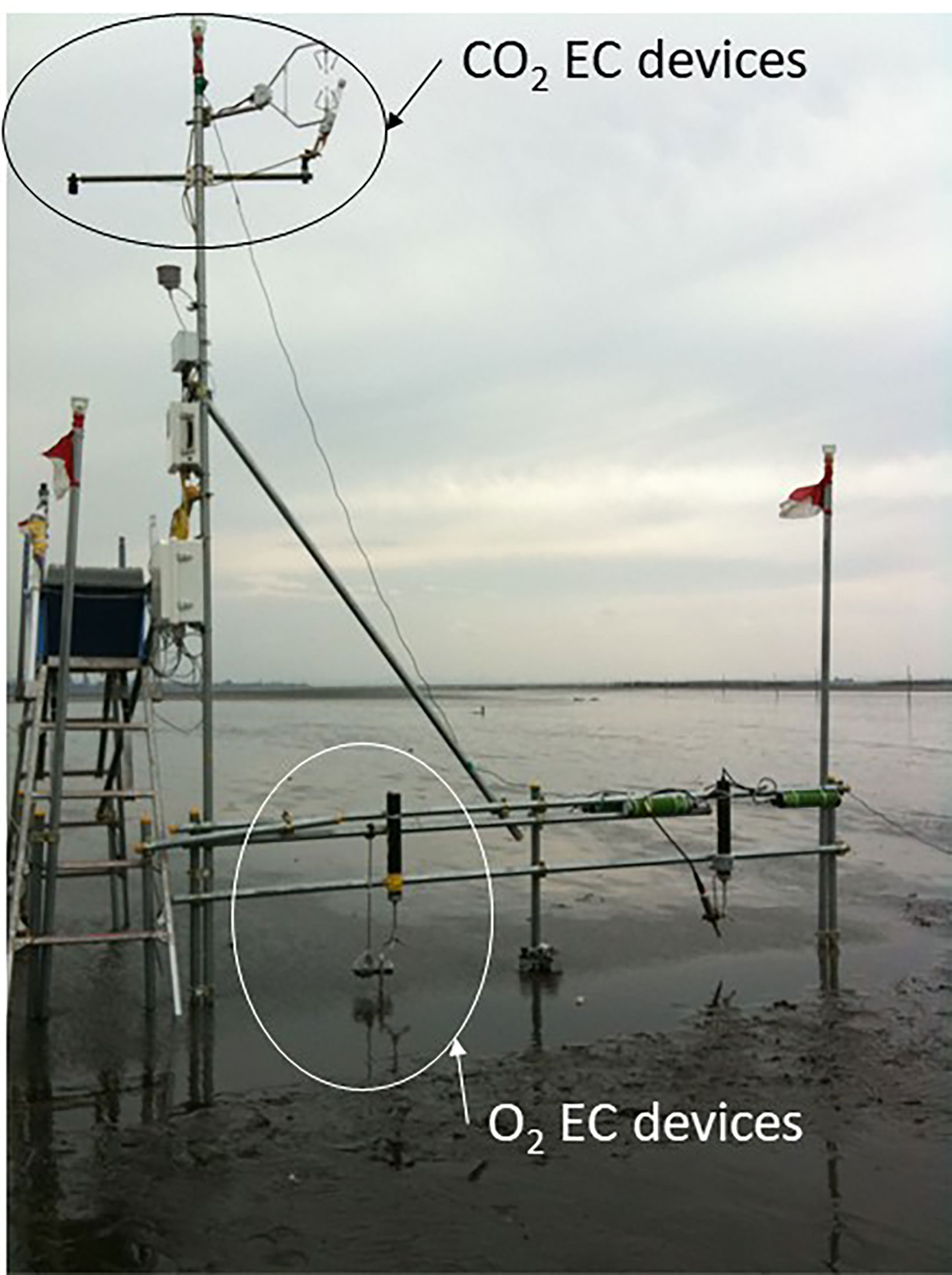
Figure 2 Platform for CO₂ EC and O₂ EC.

The EC measurements of O₂ were made only from 16:00 on 21 February to 22:30 on 24 February. The O₂ EC measurement devices were set on the platform in a direction perpendicular to the dominant direction of the tidal current to avoid artifacts during measurements (Figure 2). O₂ concentrations were measured with a Clark-type oxygen microelectrode (OX-10, Unisense). The time for a 90% response of the microelectrode to a O₂ change was less than 0.3 s. Eddy current movements were measured with an acoustic Doppler velocimeter (ADV) (Vector, Nortek). O₂ concentrations and eddy current movements were measured at a rate of 64 Hz as a precaution in the analysis of dissipation rate near sediment (not used in this study), although about 5 Hz is enough for O₂ EC measurements. The O₂ exchange was calculated every 5 minutes, and 30-minute averages were compared to CO₂ EC data. Horizontal current velocities were also measured with the ADV. Because these devices were positioned ~5 cm above the sediment surface, the measurements were invalid when the water depth was less than 5 cm.

The details of the methods used to make the other physical measurements such as water temperature, salinity, water depth, and radiation were as follows. Water temperature and salinity were measured using a thermo-salinometer (Compact-CT, JFE-Advantech) at a sampling interval of one minute. Water depth was measured using an optical O₂ sensor (Rinko, JFE-Advantech) at sampling intervals of 10 minutes; the sensor was also used to calibrate the O₂ microelectrode. Water depths were determined from the raw O₂ sensor data and one-point calibration using the tide data at Kisarazu produced by the Japan Meteorological Agency (Figure 1). Photosynthetically active radiation (PAR) was measured with a quantum sensor (LI-190, LI-COR) installed on the top of the platform (5-m height). The sampling interval for these data was one minute. The devices, except for the PAR sensor, were installed on the platform at a height of ~5 cm above the sediment surface.

The factors that determined atmospheric CO₂ exchange rates were quantified via multivariate linear analysis. Because the mechanism of CO₂ exchange on tidal flats was quite different between submerged and exposed periods, the analysis was performed separately for submerged and exposed periods. Measurements made during daytime and nighttime were analyzed separately. The effects of the variables were quantified by the partial regression coefficient of the normalized predictor variables. The predictor variables were normalized by subtracting the mean and dividing by the standard deviation of each predictor variable. The partial regression coefficient was the slope of the relationship between the normalized predictor variables (water temperature, salinity, air temperature, wind speed, PAR, water depth, current speed and O₂) and the dependent variable (CO₂ exchange). Predictor variables with larger coefficients accounted for more of the variance of the dependent variable.

Results

Twenty of the CO₂ exchange data were excluded because they were outliers based on a scaled MAD of 6.77 mmol m⁻² hour⁻¹; the remaining 338 data were used to determine atmospheric CO₂ exchange rates over the Banzu tidal flat (Figure 3). The CO₂ exchange rate (−6.05 ± 7.14 mmol m⁻² hour⁻¹, mean ± 1SD) indicates that the tidal flat was an atmospheric CO₂ sink during the measurement period. The CO₂ exchange during submerged periods (here, water depth > 0.05 m) and exposed periods were −6.51 ± 6.80 (n = 163) and −5.61 ± 7.43 mmol m⁻² hour⁻¹ (n = 175), respectively. The difference between the CO₂ exchange rates was not significant (t-test, P=0.24). The CO₂ exchange rates during daytime (here, more than 10 μmol quanta m⁻² s⁻¹ PAR) and nighttime were –8.20 ± 7.35 (n = 151) and –4.31 ± 6.48 mmol m⁻² hour⁻¹ (n = 187), respectively. The result indicates that the tidal flat absorbed atmospheric CO₂ through the day and the influx of atmospheric CO₂ was significantly greater during daytime than at night (t-test, P=4.2 × 10^-7).

FIGURE 3

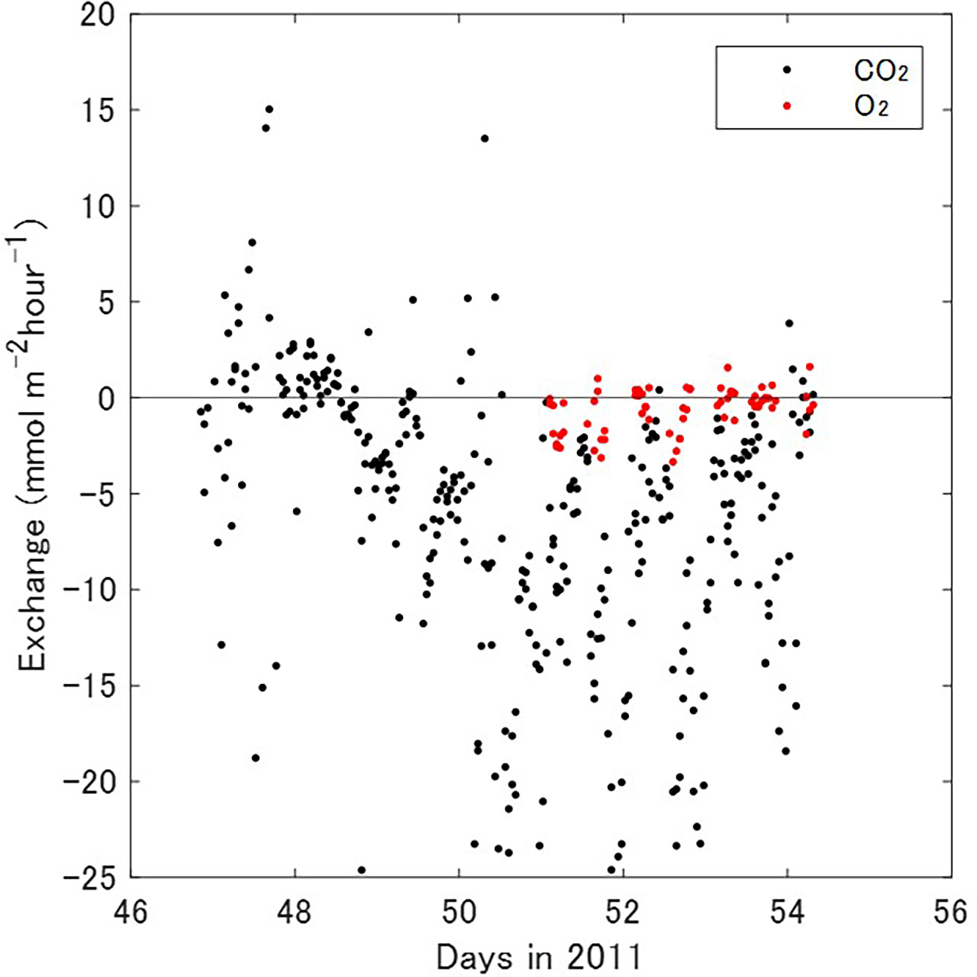
Figure 3 Temporal variations of atmospheric CO₂ (black) and O₂ (red) exchange rates measured by EC methods.

After exclusion of five outliers of the O₂ exchange data based on a scaled MAD of 1.14 mmol m⁻² hour⁻¹, the remaining 68 data were used to determine a water–sediment O₂ exchange rate of −0.62 ± 1.14 mmol m⁻² hour⁻¹. The fact that the O₂ exchange rate was negative meant that the flux of O₂ was into the sediment. The water–sediment O₂ exchange rates during daytime and nighttime were −0.63 ± 1.16 (n = 26) and −0.64 ± 1.14 mmol m⁻² hour⁻¹ (n = 42), respectively. The difference was not significant (t-test, P=0.97).

The averages and standard deviations of related predictor variables were as follows: water temperature, 9.33 ± 1.70°CC (n = 175); salinity, 28.92 ± 6.11 (n = 167); air temperature, 7.45 ± 2.39°CC (n = 279); wind speed, 5.34 ± 2.47 m s⁻¹ (n = 279); PAR, 202 ± 326 μmol quanta m⁻² s⁻¹ (n = 358); water depth, 0.19 ± 0.27 m (n = 357); current speed, 1.08 ± 0.83 cm s⁻¹ (n = 88); and dissolved O₂, 10.77 ± 0.83 mg L⁻¹ (n = 174) (Figure S1). The winds blew from the northeast during most of the measurement period (February 18–23) but blew from the south on February 17 and 24.

The estimated partial regression coefficients and adjusted coefficient of determination of each analysis are shown in Table 1 (the dependent variable is CO₂ EC exchange rate), and Table 2 shows the analogous data for O₂ EC change. Because of small number of current speed and O₂ data, these variables are not used for the CO₂ EC analysis. No multi-collinearity was detected among the predictor variables; the highest correlation coefficient between the predictor variables was 0.66 (water temperature and air temperature). The analyses were significant for CO₂ and O₂ exchange except for during the night exposed period.

TABLE 1

Table 1 Partial regression coefficients between the predictor variables and atmospheric CO2 exchange.

TABLE 2

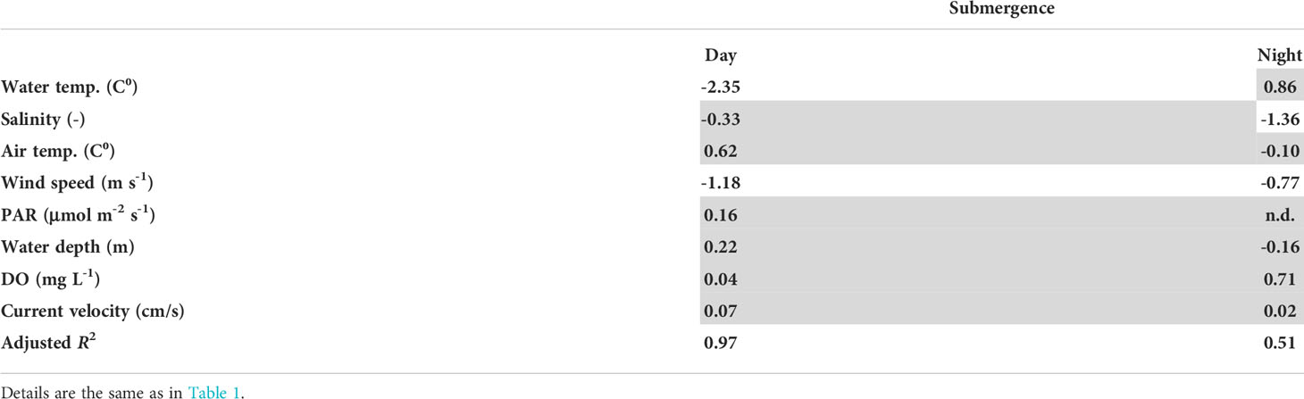
Table 2 Partial regression coefficients and coefficients of determination between the predictor variables and O2 exchange rates.

Discussion

Previous studies of CO₂ fluxes over tidal flats have reported both the absorption and release of atmospheric CO₂ (Middelburg et al., 1996; Migné et al., 2002; Spilmont et al., 2005; Klaassen and Spilmont, 2012; Sasaki et al., 2012; Otani and Endo, 2019). The causes of the differences in CO₂ exchange have been thought to include the conditions of vegetation and sediment as well as the season when the measurements were made. The influxes of atmospheric CO₂ measured in this study were consistent with the results of previous EC measurements in the Wadden Sea (Zemmelink et al., 2009), where the sediment and vegetation are similar to those at this study site. The sediments in the Wadden Sea consist of fine sand and silt, and the grain size is though to be the same or slightly smaller than at this study site. Both sites have communities of bacteria and microphytobenthos on the sediment surface. The CO₂ exchange during the submerged (high tide) and exposed (low tide) periods in the Wadden Sea were −10 and −11 mmol m⁻² hour⁻¹, respectively, during the daytime. The corresponding fluxes during the night were −0.3 and −1.0 mmol m⁻² hour⁻¹, respectively. The seawater flow from the surrounding coastal areas that generally absorbs atmospheric CO₂ is a common background of the CO₂ exchange at both sites. In addition, primary production in the water column and microbial mats on the sediment surface have been hypothesized to be the reason for atmospheric CO₂ absorption in the Wadden Sea (Zemmelink et al., 2009). Our results also indicated that the difference of atmospheric CO₂ exchange was not significant between submerged and exposed periods but was significant between daytime and nighttime. Biological activities in the water column and microbial mats might also be the main factors regulating atmospheric CO₂ exchange at our study site.

The magnitude of the rate of CO₂ uptake from the atmosphere was about 20 times larger than the magnitude of the uptake rate of 0.33 ± 0.31 mmol m⁻² hour⁻¹ in Tokyo Bay reported by Tokoro et al. (2021). The previous study by Zemmelink et al. (2009) in the Wadden Sea has likewise indicated that atmospheric CO₂ absorption measured over the tidal flat was larger than that estimated in nearby European coastal zones (< 1.4 mmol m⁻² hour⁻¹). A similarly large CO₂ exchange in near-shore areas has been observed in several coastal areas by direct measurements using floating chambers (Borges et al., 2004; Tokoro et al., 2008) and by the EC method (Rutgersson and Smedman, 2010; Tokoro et al., 2014; Ikawa and Oechel, 2015; and this study). These studies have indicated that large CO₂ exchange rates could be explained by physical turbulence near the water surface. Physical turbulence near the water surface in an area where the depth of the water exceeds the mixed layer depth is regulated only by wind speed, whereas physical turbulence in shallow areas is enhanced by factors like bottom friction and friction associated with macrophytes. Because of the absence of macrophytes and the turbulent conditions at the study site, we hypothesized that physical turbulence associated with bottom friction was the main reason for the enhancement of gas exchange in our study. Unfortunately, the quantification of the bottom friction effect was impossible in this study because the significant relationships of current speed and water depth to the CO₂ exchange were not confirmed from our measurements (Tables 1, 2). More measurements of the CO₂ exchange, depth and current speed are required for the precise analysis of atmospheric CO₂ exchange over tidal flats.

The adjusted coefficient of determination indicated that about half of the variance of the CO₂ exchange could be explained by the predictor variables. The exception was the CO₂ exchange when the sediment was exposed at night. The unexplained half of the variance might have been associated with heterogeneity inside the footprint caused by differences of tidal conditions and differences of salinity due to inputs of river water. Nonlinear relationships between the predictor variables and CO₂ exchange as well as errors in EC measurements may have accounted for the rest of the unexplained variance.

The partial regression analysis for the CO₂ EC data showed that salinity and PAR were the most significant regulating factors during submerged conditions and the daytime, respectively (Table 1). The implication was that the input of freshwater and photosynthetic uptake of CO₂ in the water and on the sediment surface regulated atmospheric CO₂ exchange over the tidal flat. The salinity decreased when the water over the tidal flat was shallow. The freshwater presumably came from the Obitsu River, which discharges from the northeast onto the tidal flat (Figure 1). The fact that the prevailing winds blew from the northeast caused part of the footprint to be easily affected by discharges from the Obitsu River. Note that the sign of the PAR coefficient differed between the periods of submergence and exposure. Because atmospheric CO₂ exchange was basically negative (influx to water or sediment), the positive coefficient was inconsistent with expectations based on photosynthetic activity. High PAR might have increased the water temperature and thereby reduced the solubility of CO₂ in the water. The result could have been a decrease of atmospheric CO₂ uptake, despite an increase of photosynthetic activity in the water during the measurement period when both water temperature and PAR were low throughout the year. Because the water temperature just below the water surface could not be measured by the thermo-salinometer, such a relationship might not be apparent from the partial regression coefficient of water temperature (−0.036 and insignificant) versus the CO₂ exchange rate during the day under submerged conditions (Table 1).

The partial regression coefficients during submergence at night were negative and positive for water temperature and air temperature, respectively. The implication is that colder water and warmer air reduced the influx of atmospheric CO₂. Because an increase of temperature with height above the water surface would stabilize the atmosphere directly over the water surface, the vertical eddy transport of CO₂ might be reduced during submergence at night on the tidal flat (Cava et al., 2004). It is possible that the same reduction of vertical eddy transport of CO₂ occurred during the period of exposure, but because the temperature near the sediment surface was not measured in this study, we can neither confirm nor reject this hypothesis.

The partial regression coefficients of O₂ fluxes estimated via EC measurements indicated that wind speed increased O₂ absorption into the sediment during both the day and night. Physical turbulence of the water therefore had more effect on atmospheric O₂ exchange than on CO₂ exchange. However, the high coefficient of determination and partial regression coefficient of water temperature during the daytime indicated that water temperature was the dominant factor that regulated O₂ exchange between the water and sediment. The implication was that photosynthetic activity on the sediment surface during the submerged period was more affected by water temperature than by other parameters like PAR. During the night, when variations of water temperature would be smaller than during the day, the effect of water temperature would be less apparent. Freshwater input would probably have decreased O₂ absorption into the sediment because a decrease of salinity might have adversely affected photosynthesis by microphytobenthos and thereby have decreased O₂ absorption. Because the variations of water temperature were smaller at night than during the day, the effects of freshwater input might be more apparent at night than during the day.

A significant correlation between air–water CO₂ fluxes and water–sediment O₂ exchange was apparent during both the day and night (Figure 4). The implication was that high rates of O₂ absorption near the sediment surface and high rates of atmospheric CO₂ absorption into the water column over the sediment occurred simultaneously. Such a relationship seems inconsistent with the biological activity of the microphytobenthos because uptake of dissolved O₂ should be accompanied by release of CO₂ into the water column and a resultant increase of the partial pressure of CO₂ in the water, and vice versa. However, the relationship seems consistent with biological activity in the water column, wherein photosynthetic activity leads to absorption of atmospheric CO₂ and release of dissolved O₂, and vice versa. The decrease of CO₂ and increase of O₂ concentrations in the water column would cause an increase of the downward CO₂ (air to water) and O₂ (water to sediment) fluxes because the concentration gradients would increase at each boundary layer. Physical turbulence could enhance that relationship. An increase of wind speed or bottom friction could enhance both air–water CO₂ fluxes and water–sediment O₂ exchange via physical turbulence. Resuspension of sediment in the low-O₂ layer by physical disturbance would also increase the O₂ concentration gradient in the water. Unfortunately, the limited number of O₂ EC measurements in this study precluded further testing of this hypothesis. Additional O₂ EC data will be required for a more detailed analysis.

FIGURE 4

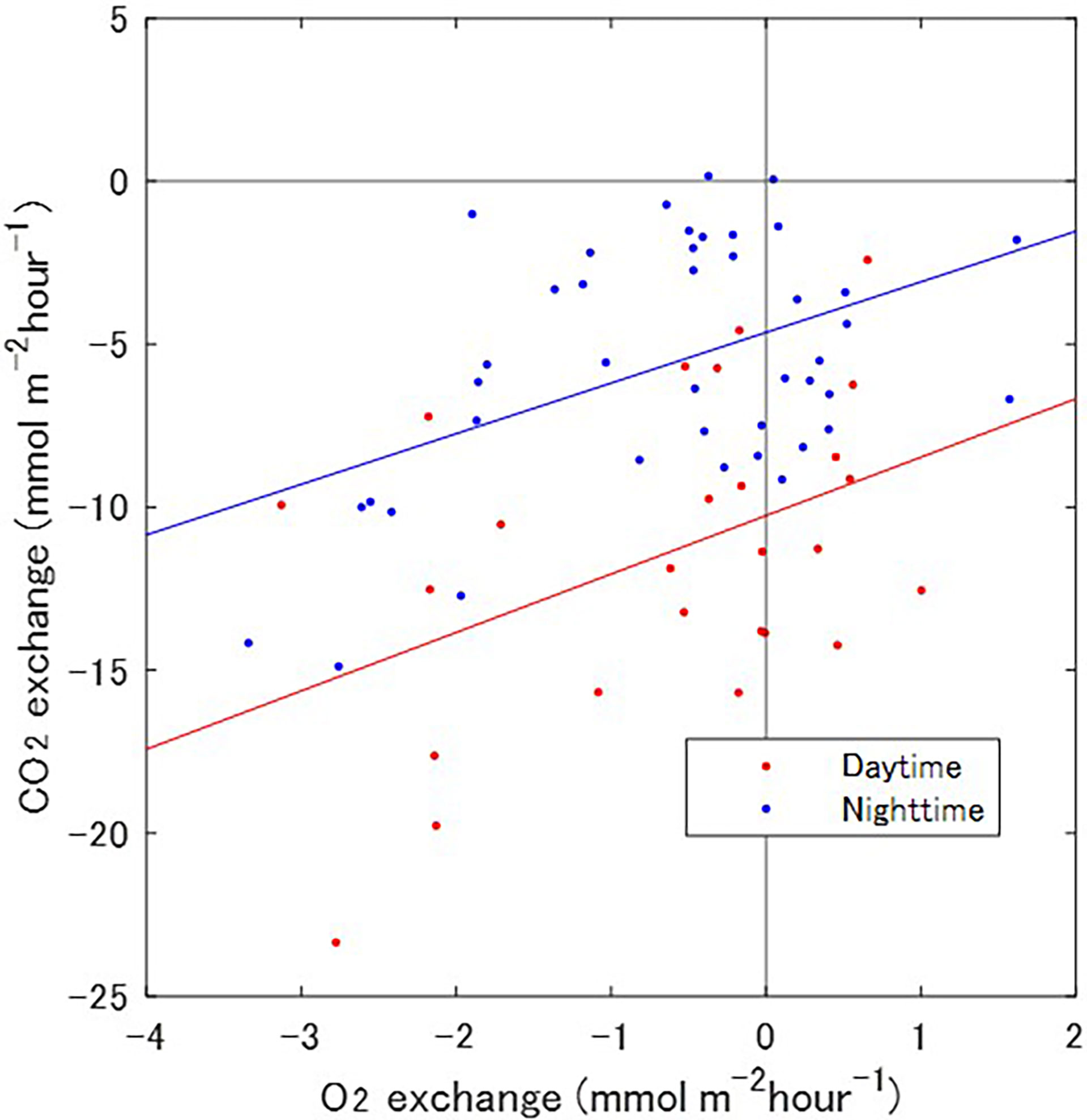
Figure 4 Comparison between atmospheric CO₂ and O₂ exchange rates. The red and blue dots indicate exchange rates during daytime and nighttime, respectively. The red and blue lines are the linear regressions between the two rates during the daytime (R² = 0.44, p = 0.03) and nighttime data (R² = 0.47, p = 0.002).

Summary

The mechanisms associated with the atmospheric CO₂ exchange on a tidal flat measured in this study could be summarized as follows. (1) The tidal flat in Tokyo Bay and the Wadden Sea are both sinks for atmospheric CO₂. In both cases, there are no macrophytes, and the sediment is composed mainly of fine sand. (2) Air–water CO₂ fluxes over the tidal flat were about 20 times the fluxes in Tokyo Bay. The likely explanation is enhancement by tide-driven factors. (3) Freshwater input and PAR were important factors that regulated CO₂ exchange during submergence and the daytime, respectively. (4) A stable atmospheric layer near the water/sediment surface might have reduced atmospheric CO₂ exchange during the night. (5) O₂ exchange was affected by physical turbulence caused by wind over the water/sediment surface. O₂ absorption into the sediment would be increased by warm water and decreased by freshwater inputs during the daytime and nighttime, respectively. (6) Photosynthetic activity in water and physical turbulence increased atmospheric CO₂ absorption and the supply of O₂ to the sediment surface. This study was limited to several days in the winter, and annual measurements by EC methods are expected to provide more understanding of the carbon flow over tidal flats surrounding urbanized areas like Tokyo Bay.

Data availability statement

The original contributions presented in the study are included in the article/Supplementary Material. Further inquiries can be directed to the corresponding author.

Author contributions

Conceived and designed: TT and TK. Performed field work: TT. Analyzed the data: TT and TK. Writing led by TT.

Funding

This study was supported by a Grant-in-Aid for Scientific Research (no. 18H04156) from the Japan Society for the Promotion of Science.

Acknowledgments

We thank S. Hosokawa and E. Miyoshi for help with the field work. We also thank K. Watanabe for help with the referential work.

Conflict of interest

The authors declare that the research was conducted in the absence of any commercial or financial relationships that could be construed as a potential conflict of interest.

Publisher’s note

All claims expressed in this article are solely those of the authors and do not necessarily represent those of their affiliated organizations, or those of the publisher, the editors and the reviewers. Any product that may be evaluated in this article, or claim that may be made by its manufacturer, is not guaranteed or endorsed by the publisher.

Supplementary material

The Supplementary Material for this article can be found online at: https://www.frontiersin.org/articles/10.3389/fmars.2022.989270/full#supplementary-material

Supplementary Figure 1 | Temporal variations of water temperature, salinity, air temperature, wind speed, water depth, PAR, current speed, and O₂ concentration during the measurement.

References

Berg P., Huettel M., Glud R. N., Reimers C. E., Attard K. M. (2022). Aquatic eddy covariance: The method and its contributions to defining oxygen and carbon fluxes in marine environments. Annu. Rev. Mar. Sci. 14, 431–455. doi: 10.1146/annurev-marine-042121-012329

CrossRef Full Text | Google Scholar

Blomquist B. W., Huebert B. J., Fairall C. W., Bariteau L., Edson J. B., Hare J. E., et al. (2014). Advances in air-Sea flux measurement by eddy correlation. Boundary-Layer Meteorol. 152 (3), 245–276. doi: 10.1007/s10546-014-9926-2

CrossRef Full Text | Google Scholar

Borges A. V., Delille B., Frankignoulle M. (2005). Budgeting sinks and sources of CO₂ in the coastal ocean: Diversity of ecosystems counts. Geophys. Res. Lett. 32 (14), L14601. doi: 10.1029/2005GL023053

CrossRef Full Text | Google Scholar

Borges A. V., Delille B., Schiettecatte L. S., Gazeau F., Abril G., Frankignoulle M. (2004). Gas transfer velocities of CO₂ in three European estuaries (Randers fjord, scheldt, and Thames). Limnol. Oceanog. 49 (5), 1630–1641. doi: 10.4319/lo.2004.49.5.1630

CrossRef Full Text | Google Scholar

Cava D., Giostra U., Siqueira M., Katul G. (2004). Organised motion and radiative perturbations in the nocturnal canopy sublayer above an even-aged pine forest. Boundary-Layer Meteorol. 112 (1), 129–157. doi: 10.1023/B:BOUN.0000020160.28184.a0

CrossRef Full Text | Google Scholar

Edson J. B., Fairall C. W., Bariteau L., Zappa C. J., Cifuentes-Lorenzen A., McGillis W. R., et al. (2011). Direct covariance measurement of CO₂ gas transfer velocity during the 2008 southern ocean gas exchange experiment: Wind speed dependency. J. Geophys. Research-Oceans 116, C00f10. doi: 10.1029/2011jc007022

CrossRef Full Text | Google Scholar

Endo T., Otani S. (2019). “Carbon storage in tidal flats,” in Blue carbon in shallow coastal ecosystems: Carbon dynamics, policy, and implementation. Eds. Kuwae T., Hori. M. (Singapore: Springer Singapore), 129–151.

Google Scholar

Frankignoulle M. (1988). Field-measurements of air Sea CO₂ exchange. Limnol. Oceanog. 33 (3), 313–322. doi: 10.4319/lo.1988.33.3.0313

CrossRef Full Text | Google Scholar

Hosokawa Y. (1999). Water purification system at coastal tidal flat and possibility of its rehabilitations and construction. Bull. Coast. Oceanog. 36 (2), 137–144. doi: 10.32142/engankaiyo.36.2_137

CrossRef Full Text | Google Scholar

Ikawa H., Oechel W. C. (2015). Temporal variations in air-sea CO₂ exchange near large kelp beds near San Diego, California. J. Geophys. Research-Oceans 120 (1), 50–63. doi: 10.1002/2014jc010229

CrossRef Full Text | Google Scholar

Kayanne H., Suzuki A., Saito H. (1995). Diurnal changes in the partial-pressure of carbon-dioxide in coral-reef water. Science 269 (5221), 214–216. doi: 10.1126/science.269.5221.214

PubMed Abstract | CrossRef Full Text | Google Scholar

Klaassen W., Spilmont N. (2012). Inter-annual variability of CO₂ exchanges between an emersed tidal flat and the atmosphere. Estuar. Coast. Shelf Sci. 100, 18–25. doi: 10.1016/j.ecss.2011.06.002

CrossRef Full Text | Google Scholar

Kljun N., Calanca P., Rotach M. W., Schmid H. P. (2004). A simple parameterisation for flux footprint predictions. Boundary-Layer Meteorol. 112 (3), 503–523. doi: 10.1023/B:Boun.0000030653.71031.96

CrossRef Full Text | Google Scholar

Kondo F., Ono K., Mano M., Miyata A., Tsukamoto O. (2014). Experimental evaluation of water vapour cross-sensitivity for accurate eddy covariance measurement of CO₂ flux using open-path CO₂/H2O gas analysers. Tellus Ser. B-Chemical Phys. Meteorol. 66, 23803. doi: 10.3402/tellusb.v66.23803

CrossRef Full Text | Google Scholar

Kubo A., Maeda Y., Kanda J. (2017). A significant net sink for CO₂ in Tokyo bay. Sci. Rep. 7, 44355. doi: 10.1038/srep44355

PubMed Abstract | CrossRef Full Text | Google Scholar

Kuwae T., Kamio K., Inoue T., Miyoshi E., Uchiyama Y. (2006). Oxygen exchange flux between sediment and water in an intertidal sandflat, measured in situ by the eddy-correlation method. Mar. Ecol. Prog. Ser. 307, 59–68. doi: 10.3354/meps307059

CrossRef Full Text | Google Scholar

Landwehr S., Miller S. D., Smith M. J., Saltzman E. S., Ward B. (2014). Analysis of the PKT correction for direct CO₂ flux measurements over the ocean. Atmos. Chem. Phys. 14 (7), 3361–3372. doi: 10.5194/acp-14-3361-2014

CrossRef Full Text | Google Scholar

Lee X., Massman W. J., Law B. (2004). Handbook of micrometeorology: A guide for surface flux measurement and analysis (Atmospheric and oceanographic sciences library (Dordrecht Netherlands: Springer Netherlands).

Google Scholar

Mørk E. T., Sorensen L. L., Jensen B., Sejr M. K. (2014). Air-Sea gas transfer velocity in a shallow estuary. Boundary-Layer Meteorol. 151 (1), 119–138. doi: 10.1007/s10546-013-9869-z

CrossRef Full Text | Google Scholar

Massman W. J. (2000). A simple method for estimating frequency response corrections for eddy covariance systems. Agric. For. Meteorol. 104 (3), 185–198. doi: 10.1016/S0168-1923(00)00164-7

CrossRef Full Text | Google Scholar

Mateo M. A., Romero J., Perez M., Littler M. M., Littler D. S. (1997). Dynamics of millenary organic deposits resulting from the growth of the Mediterranean seagrass Posidonia oceanica. Estuar. Coast. Shelf Sci. 44 (1), 103–110. doi: 10.1006/ecss.1996.0116

CrossRef Full Text | Google Scholar

Mcleod E., Chmura G. L., Bouillon S., Salm R., Björk M., Duarte C. M., et al. (2011). A blueprint for blue carbon: toward an improved understanding of the role of vegetated coastal habitats in sequestering CO₂. Front. Ecol. Environ. 9 (10), 552–560. doi: 10.1890/110004

CrossRef Full Text | Google Scholar

McMillen R. T. (1988). An eddy-correlation technique with extended applicability to non-simple terrain. Boundary-Layer Meteorol. 43 (3), 231–245. doi: 10.1007/Bf00128405

CrossRef Full Text | Google Scholar

Middelburg J. J., Klaver G., Nieuwenhuize J., Wielemaker A., deHaas W., Vlug T., et al. (1996). Organic matter mineralization in intertidal sediments along an estuarine gradient. Mar. Ecol. Prog. Ser. 132 (1-3), 157–168. doi: 10.3354/meps132157

CrossRef Full Text | Google Scholar

Migné A., Davoult D., Spilmont N., Menu D., Boucher G., Gattuso J. P., et al. (2002). A closed-chamber CO₂-flux method for estimating intertidal primary production and respiration under emersed conditions. Mar. Biol. 140 (4), 865–869. doi: 10.1007/s00227-001-0741-1

CrossRef Full Text | Google Scholar

Murray N. J., Phinn S. R., DeWitt M., Ferrari R., Johnston R., Lyons M. B., et al. (2019). The global distribution and trajectory of tidal flats. Nature 565 (7738), 222–22+. doi: 10.1038/s41586-018-0805-8

PubMed Abstract | CrossRef Full Text | Google Scholar

Nellemann C., Corcoran E., Duarte C. M., Valdrés L., De Young C., Fonseca L., et al. (2009). Blue carbon: the role of healthy oceans in binding carbon: a rapid response assessment (Arendal, Norway: GRID-Arendal for United Nations Environment Programme).

Google Scholar

O'connor D. J., Dobbins W. E. (1958). Mechanism of reaeration in natural streams. Trans. Am. Soc. Civil Eng. 123, 641–666. doi: 10.1061/TACEAT.0007609

CrossRef Full Text | Google Scholar

Otani S., Endo T. (2019). “CO2 flux in tidal flats and salt marshes,” in Blue carbon in shallow coastal ecosystems: Carbon dynamics, policy, and implementation. Eds. Kuwae T., Hori. M. (Singapore: Springer Singapore), 223–250.

Google Scholar

Polsenaere P., Lamaud E., Lafon V., Bonnefond J. M., Bretel P., Delille B., et al. (2012). Spatial and temporal CO₂ exchanges measured by eddy covariance over a temperate intertidal flat and their relationships to net ecosystem production. Biogeosciences 9 (1), 249–268. doi: 10.5194/bg-9-249-2012

CrossRef Full Text | Google Scholar

Prytherch J., Yelland M. J., Pascal R. W., Moat B. I., Skjelvan I., Neill C. C. (2010). Direct measurements of the CO₂ flux over the ocean: Development of a novel method. Geophys. Res. Lett. 37, L03607. doi: 10.1029/2009gl041482

CrossRef Full Text | Google Scholar

Raymond P. A., Cole J. J. (2001). Gas exchange in rivers and estuaries: Choosing a gas transfer velocity. Estuaries 24 (2), 312–317. doi: 10.2307/1352954

CrossRef Full Text | Google Scholar

Rousseeuw P. J., Croux C. (1993). Alternatives to the median absolute deviation. J. Am. Stat. Assoc. 88 (424), 1273–1283. doi: 10.2307/2291267

CrossRef Full Text | Google Scholar

Rutgersson A., Smedman A. (2010). Enhanced air-sea CO₂ transfer due to water-side convection. J. Mar. Syst. 80 (1-2), 125–134. doi: 10.1016/j.jmarsys.2009.11.004

CrossRef Full Text | Google Scholar

Sanders C. J., Smoak J. M., Naidu A. S., Sanders L. M., Patchineelam S. R. (2010). Organic carbon burial in a mangrove forest, margin and intertidal mud flat. Estuar. Coast. Shelf Sci. 90 (3), 168–172. doi: 10.1016/j.ecss.2010.08.013

CrossRef Full Text | Google Scholar

Sasaki A., Hagimori Y., Yuasa I., Nakatsubo T. (2012). Annual sediment respiration in estuarine sandy intertidal flats in the seto inland Sea, Japan. Landscape Ecol. Eng. 8 (1), 107–114. doi: 10.1007/s11355-011-0157-0

CrossRef Full Text | Google Scholar

Spilmont N., Migné A., Lefebvre A., Artigas L. F., Rauch M., Davoult D. (2005). Temporal variability of intertidal benthic metabolism under emersed conditions in an exposed sandy beach (Wimereux, eastern English channel, France). J. Sea Res. 53 (3), 161–167. doi: 10.1016/j.seares.2004.07.004

CrossRef Full Text | Google Scholar

Tokoro T., Hosokawa S., Miyoshi E., Tada K., Watanabe K., Montani S., et al. (2014). Net uptake of atmospheric CO₂ by coastal submerged aquatic vegetation. Global Change Biol. 20 (6), 1873–1884. doi: 10.1111/gcb.12543

CrossRef Full Text | Google Scholar

Tokoro T., Kayanne H., Watanabe A., Nadaoka K., Tamura H., Nozaki K., et al. (2008). High gas-transfer velocity in coastal regions with high energy-dissipation rates. J. Geophys. Research-Oceans 113, C11006. doi: 10.1029/2007jc004528

CrossRef Full Text | Google Scholar

Tokoro T., Kuwae T. (2018). Improved post-processing of eddy-covariance data to quantify atmosphere-aquatic ecosystem CO₂ exchanges. Front. Mar. Sci. 5. doi: 10.3389/fmars.2018.00286

CrossRef Full Text | Google Scholar

Tokoro T., Nakaoka S., Takao S., Kuwae T., Kubo A., Endo T., et al. (2021). Contribution of biological effects to carbonate-system variations and the air-water CO₂ flux in urbanized bays in Japan. J. Geophys. Research-Oceans 126, e2020JC016974. doi: 10.1029/2020JC016974

CrossRef Full Text | Google Scholar

Uchiyama Y. (2007). Hydrodynamics and associated morphological variations on an estuarine intertidal sand flat. J. Coast. Res. 23 (4), 1015–1027. doi: 10.2112/04-0336.1

CrossRef Full Text | Google Scholar

Vesala T., Eugster W., Ojala A. (2012). “Eddy covariance measurements over lakes,” in Eddy covariance: A practical guide to measurement and data analysis. Eds. Aubinet M., Vesala T., Papale D. (Dordrecht: Springer Netherlands), 365–376.

Google Scholar

Webb E. K., Pearman G. I., Leuning R. (1980). Correction of flux measurements for density effects due to heat and water-vapor transfer. Q. J. R. Meteorol. Soc. 106 (447), 85–100. doi: 10.1002/qj.49710644707

CrossRef Full Text | Google Scholar

Widdows J., Blauw A., Heip C. H. R., Herman P. M. J., Lucas C. H., Middelburg J. J., et al. (2004). Role of physical and biological processes in sediment dynamics of a tidal flat in westerschelde estuary, SW Netherlands. Mar. Ecol. Prog. Ser. 274, 41–56. doi: 10.3354/meps274041

CrossRef Full Text | Google Scholar

Zemmelink H. J., Slagter H. A., van Slooten C., Snoek J., Heusinkveld B., Elbers J., et al. (2009). Primary production and eddy correlation measurements of CO₂ exchange over an intertidal estuary. Geophys. Res. Lett. 36, L19606. doi: 10.1029/2009gl039285

CrossRef Full Text | Google Scholar