 John M. O’Brien
 Melisa C. Wong
 Ryan R.E. Stanley
- Bedford Institute of Oceanography, Fisheries and Oceans Canada, Dartmouth, NS, Canada
Baseline data on the distribution and extent of biogenic habitat-forming species at a high spatial resolution are essential to inform habitat management strategies, preserve ecosystem integrity, and achieve effective conservation objectives in the nearshore. Model-based approaches to map suitable habitat for these species are a key tool to address this need, filling in gaps where observations are otherwise unavailable and remote sensing methods are limited by turbid waters or cannot be applied at scale. We developed a high resolution (35 m) ensemble species distribution model to predict the distribution of eelgrass (Zostera marina) along the Atlantic coast of Nova Scotia, Canada where the observational coverage of eelgrass occurrence is sparse and nearshore waters are optically complex. Our ensemble model was derived as a performance-weighted average prediction of 7 different modeling methods fit to 6 physical predictors (substrate type, depth, wave exposure, slope, and two bathymetric position indices) and evaluated with a 5-fold spatially-blocked cross-validation procedure. The ensemble model showed moderate predictive performance (Area Under the Receiver-Operating Characteristic Curve (AUC) = 0.803 ± 0.061, True Skill Statistic (TSS) = 0.531 ± 0.100; mean ± SD), high sensitivity (92.0 ± 4.5), and offered some improvement over individual models. Substrate type, depth, and relative wave exposure were the most influential predictors associated with eelgrass occurrence, where the highest probabilities were associated with sandy and sandy-mud sediments, depths ranging 0 m – 4 m, and low to intermediate wave exposure. Within our study region, we predicted a total extent of suitable eelgrass habitat of 38,130 ha. We found suitable habitat was particularly extensive within the long narrow inlets and extensive shallow flats of the South Shore, Eastern Shore, and Bras d’Or Lakes. We also identified substantial overlap of eelgrass habitat with previously identified Ecologically and Biologically Significant Areas that guide regional conservation planning while also highlighting areas of greater prediction uncertainty arising from disagreement among modeling methods. By offering improved sensitivity and insights into the fine-scale regional distribution of a habitat-forming species with associated uncertainties, our ensemble-based modeling approach provides improved support to numerous nearshore applications including conservation planning and restoration, marine spatial and emergency response planning, environmental impact assessments, and fish habitat protection.
Introduction
Large marine macrophytes such as seagrasses, kelps, and mangroves provide important biogenic habitat in nearshore ecosystems (Norderhaug et al., 2012; Rodil et al., 2021) that generate substantial primary production (Cebrian, 1999) and high rates of detrital export that subsidize adjacent ecosystems (Cebrian, 1999; Krumhansl and Scheibling, 2012). However, alarming global trends of decline have been observed across major coastal biogenic habitats (Waycott et al., 2009; Krumhansl et al., 2016; Goldberg et al., 2020; Dunic et al., 2021) and projected climate-mediated range reductions driven by loss of suitable coastal habitat and warm-edge contractions outpace poleward expansion (Record et al., 2013; Chefaoui et al., 2018; Wilson and Lotze, 2019; Wilson et al., 2019b). These reductions threaten seagrass and kelp habitats and their continued provision of ecosystem services (Smale et al., 2013; Namba et al., 2018). Economic value of services provided by seagrasses, kelp beds, and mangroves, such as coastal protection, nutrient cycling, fisheries production, recreational opportunities, and carbon sequestration, range from $100s − $100,000s USD ha-1 yr-1 (Barbier et al., 2011; Dewsbury et al., 2016; Himes-Cornell et al., 2018; Eger et al., 2021). Consequently, there is strong motivation behind ambitious calls for habitat protection and restoration (van Katwijk et al., 2016; Eger et al., 2020; Buelow et al., 2022). These strong ecological and economic rationales for protection, however, are juxtaposed with a lack of fine-scale data on the distribution and extent of these important ecosystems at regional scales, which hinders the application and success of conservation planning and targeted habitat rehabilitation programs.
Optical and hydroacoustic remote sensing methods have been widely adopted for mapping shallow submerged aquatic vegetation (SAV) in the nearshore at relatively fine spatial resolutions (cm – 10s m), but limitations and trade-offs among the range of techniques preclude a universal solution for all monitoring and management applications (Rowan and Kalacska, 2021). Differences among optical remote sensing platforms impose trade-offs between resolution (spatial, temporal, and spectral), extent (spatial and temporal), and start-up costs (Cavanaugh et al., 2021). For example, while freely available Landsat imagery has been used to map regional scale distributions (Torres-Pulliza et al., 2013) and historic trends of seagrasses (Knudby et al., 2010), the larger pixel size and lower spectral resolution limits the ability of this system to discriminate species (Phinn et al., 2008), functional benthic groups (Knudby et al., 2010; Torres-Pulliza et al., 2013) or to detect sparse vegetation (Phinn et al., 2008; Torres-Pulliza et al., 2013). In contrast, hyperspectral and commercial multispectral sensors can map abundance and species composition of SAV at a high spatial resolution (m’s), although they are largely restricted to smaller spatial extents (bays or estuaries) and optically shallow water (< 2 − 3 m) (Phinn et al., 2008; Hill et al., 2014; Roelfsema et al., 2014; Vahtmäe et al., 2020). The rapid attenuation of light with depth obscures the spectral reflectance from benthic vegetation, which is exacerbated in turbid waters (Vahtmäe et al., 2020; Cavanaugh et al., 2021). Furthermore, mismatches between patch and landscape characteristics with sensor radiometric and spatial resolution can hinder the detection of sparse or patchy vegetation by even high-resolution multispectral and hyperspectral systems (Phinn et al., 2008; Barrell et al., 2015; Vahtmäe et al., 2020). Acoustic mapping methods using side scan sonar, single- or multi-beam echosounders can produce high-resolution maps of SAV distribution and abundance, and are not limited by turbidity (Komatsu et al., 2002; Gumusay et al., 2019) or some of the detection-limit issues of optical methods (Barrell et al., 2015). However, they are generally limited in the spatial extent of application (ha – 1000s ha). Therefore, the ability of remote sensing methods to produce high-resolution maps of submerged macrophytes at large regional scales may be challenged in turbid, temperate coastal waters where vegetated habitats exist in patchy mosaics and across broad depth gradients.
Advances in predictive habitat mapping and species distribution models (i.e., ecological niche or habitat suitability models) offer complementary approaches for evaluating the distribution and extent of SAV and other biogenic habitats that circumvent some of the limitations of remote sensing, while providing additional advantages. Species distribution models (SDMs) relate discontinuous species occurrence records to environmental covariates using a variety of regression or machine learning techniques, enabling continuous predictions of distributions over large spatial extents (Guisan & Zimmermann, 2000; Elith et al., 2006). This predictive power facilitates the mapping of distributions far beyond depth limits of remote sensing techniques (e.g., the deep-sea; Knudby et al., 2010) or in other environments where sampling is logistically difficult and remote sensing is challenged such as the Arctic (Jenkins et al., 2020; Goldsmit et al., 2021) or turbid coastal waters (Schubert et al., 2015). SDMs also permit hindcasts to paleoclimatic conditions (Chefaoui et al., 2017; Assis et al., 2018) or forecasts to future climate scenarios (Valle et al., 2014; Wilson and Lotze, 2019; Wilson et al., 2019b; Hu et al., 2021) to predict past distributions and projected range shifts, respectively. In addition, SDM methods provide other useful insights into species-environment relationships including identifying the environmental variables that most constrain species occurrence (Breiman, 2001), characterizing the marginal effects of these variables (Elith et al., 2005), and mapping uncertainty associated with the model predictions (e.g., Beazley et al., 2021).
Despite the potential for SDM techniques to guide management practices for SAV in the nearshore (e.g., prioritization of areas for conservation within coastal Marine Spatial Planning - MSP), a lack of consistency in predictions among modeling methods may detract from confident management decisions. Even as the range of modeling methods has proliferated rapidly (Guisan and Zimmermann, 2000; Elith et al., 2006), the overall performance (Elith et al., 2006; Dormann et al., 2008; Grenouillet et al., 2011; Guo et al., 2015) and spatial predictions (Pearson et al., 2006; Dormann et al., 2008; Ochoa-Ochoa et al., 2016) can vary widely among modeling approaches. While particular species characteristics (e.g., prevalence, geographic and environmental range, genetic variation) are known to effect model performance (Segurado and Araújo, 2004; Grenouillet et al., 2011; Guo et al., 2015; Lowen et al., 2019), there remains little practical guidance to inform model selection based on optimized performance for particular species groups (Segurado and Araújo, 2004; Elith et al., 2006), regional contexts (Elith et al., 2006), or intended model applications (Elith and Graham, 2009). In light of this variation, ensemble models that average the predictions of numerous methods have been proposed (Araújo and New, 2007). These ensemble-based modeling approaches incorporate the predication variability among different modeling methods to produce a combined SDM that in many cases offers improvement over individual models (Meller et al., 2014). This approach is particularity advantageous when applied over a wide range of environmental conditions where prediction accuracy associated with boundary conditions (e.g., environmental extremes) can be limited (Grenouillet et al., 2011). Despite these advantages and evidence for improved performance of ensemble-based approaches (Grenouillet et al., 2011; Guo et al., 2015), there has been considerably less uptake by marine SDM studies compared to terrestrial environments (Hao et al., 2019). The few examples of ensemble models for seagrasses (Chefaoui et al., 2016; Chefaoui et al., 2017; Chefaoui et al., 2018; Chefaoui et al., 2021) and kelps (Goldsmit et al., 2021) have demonstrated the potential applications of this approach for SAV and often highlight improved performance compared to individual models. These studies made use of widely available climatic predictors for ensemble construction and projections; consistent with the typical application of ensemble models (Hao et al., 2019). However, the relatively coarse spatial resolution of these predictors abstracts from the scale required for local conservation planning and habitat management. Furthermore, these studies generally modelled species with relatively restricted geographic ranges, which are known to yield higher accuracy and greater consensus among models compared to widely distributed species and habitat generalists (Segurado and Araújo, 2004; Grenouillet et al., 2011).
Among seagrass species, eelgrass (Zostera marina) occupies the largest geographic range and exhibits a broad environmental niche (Blok et al., 2018), complicating the task of regional habitat managers to identify priority areas. In eastern Canada, located centrally within its Northwest Atlantic range, eelgrass is considered an ecologically significant species (DFO, 2009), provides nursery habitat to juvenile fish (Laurel et al., 2003; Warren et al., 2010), and may enhance benthic secondary production (Wong, 2018). Because of this biogenic habitat value, eelgrass has been prioritized in regional conservation planning (DFO, 2018) and habitat protection guidelines (DFO, 2012) and benefits from additional risk mitigation with respect to fish habitat outlined in Canada’s Fisheries Act. However, effective protection measures are impeded by large regional gaps in the observed distribution and extent of eelgrass. For example, along the Atlantic coast of Nova Scotia, eelgrass occurrence records are patchy and remote sensing mapping efforts have been relatively limited in spatial extent (Vandermeulen, 2014; Wilson et al., 2019a; Wilson et al., 2020). Detection of eelgrass with satellite imagery in this region has also proved challenging due to the optical complexity of coastal waters (Wilson et al., 2019a; Wilson et al., 2020), mixed occurrences with subtidal seaweeds (O’Brien & Wong unpubl.), and the broad gradients in depth and environmental conditions occupied by eelgrass (Wong, 2018; Krumhansl et al., 2020). Under these circumstances, species distribution modeling using an ensemble approach is particularly well-suited for mapping the distribution and extent of eelgrass at a scale and resolution required by regional conservation planners.
Here, we use ensemble modeling approaches to identify suitable habitat for a widely distributed species within a subset of its known range at a high spatial resolution and evaluate the predicted distribution with respect to existing areas prioritized for conservation and management. Specifically, we develop and evaluate the performance of an ensemble species distribution model for eelgrass, Zostera marina, along the Atlantic coast of Nova Scotia Canada. Next, we use the fine-scale spatial predictions of the ensemble model (35-m nominal resolution) to evaluate coastal scale patterns in the probability of eelgrass occurrence, the distribution and extent of suitable habitat, overlap with designated Ecologically and Biologically Significant Areas (EBSAs) used for marine conservation planning, and highlight spatial variation in model uncertainty. Finally, we use other model interpretation methods (permutation importance, response plots) to distinguish relevant environmental features of suitable eelgrass habitat. In particular, we identify the most influential environmental covariates with eelgrass regional distribution and characterize the change in probability of occurrence along those key gradients. Our study highlights the capabilities of an ensemble approach to species distribution modeling for evaluating the distribution of submerged aquatic vegetation at a relatively high spatial resolution. These model predictions can be applied for conservation planning and monitoring of nearshore habitats, particularly in areas where remote sensing techniques are limited.
Methods
Study area and model domain
We developed an ensemble species distribution model for eelgrass (Zostera marina) along the Atlantic coast of Nova Scotia within a spatial domain spanning ~ 3.5° latitude from Cape Sable Island (43.4905° N, 65.6214° W) to Cape North (47.0295° N, 60.3921° W; Figure 1). This expanse of the inshore Scotian Shelf is characterized by extensive bedrock outcrops with thin sand and gravel deposits occurring throughout and infill of mud constrained mainly to deep basins and inner harbours (Bundy et al., 2014). The predominantly rocky shoreline is intersected by large bays, long and narrow inlets, salt marsh and sandy beaches (Bundy et al., 2014). Human impacts to eelgrass beds in this region are relatively low in comparison to other areas of Atlantic Canada (Murphy et al., 2019). We excluded the Bay of Fundy because environmental conditions diverge considerably in comparison to the Atlantic coast (Greenlaw et al., 2012) and eelgrass is uncommon owing to extreme tidal ranges, high sediment loads, and steep coastline topography (Murphy et al., 2021). We further constrained the model domain to the 12-m depth contour and within 5 km from shore (Figure 1). This boundary captures the regional published depth limit of eelgrass (DFO, 2009) and distinguishes the shallow nearshore from deeper subtidal areas.
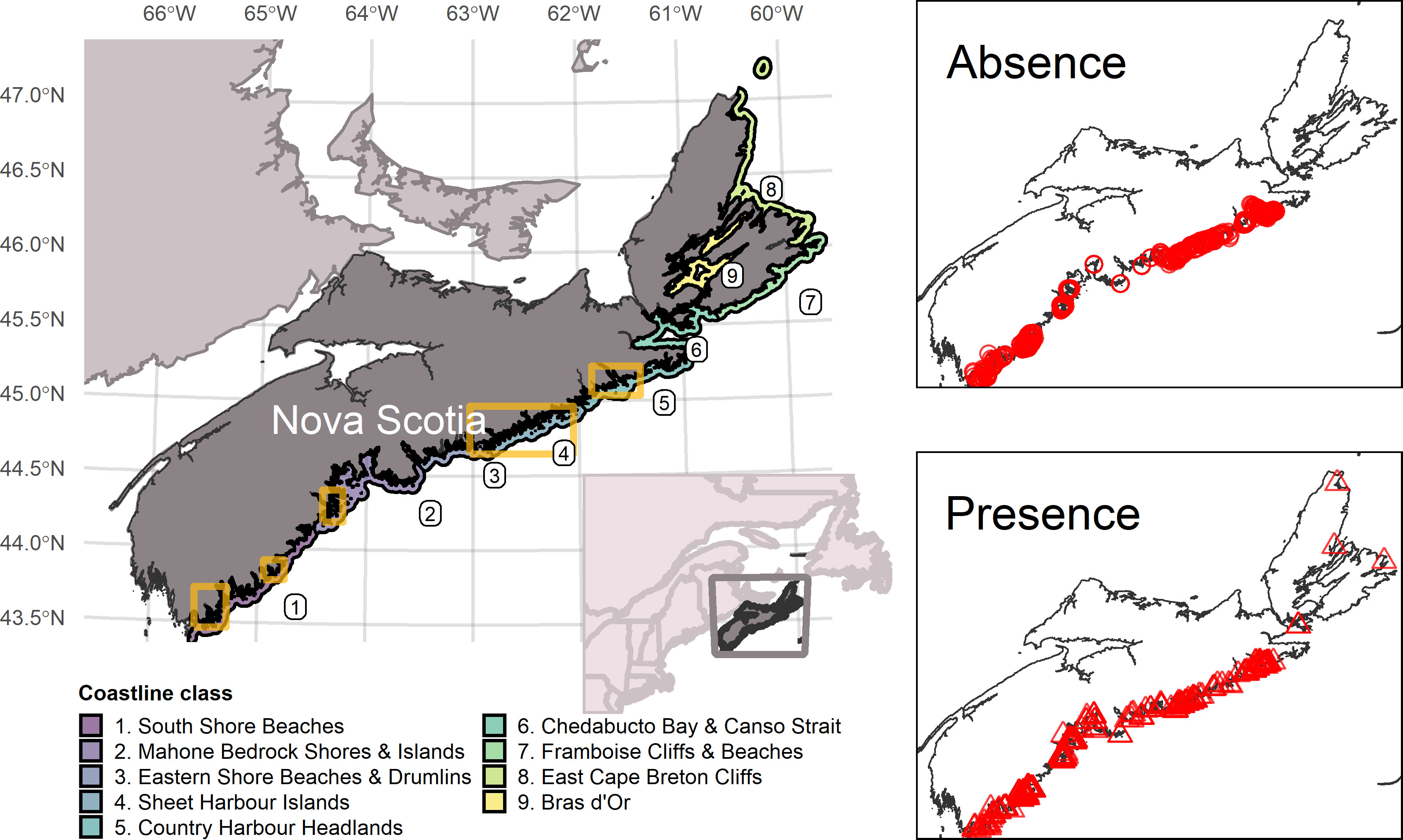
Figure 1 Study area extent along the Atlantic coast of Nova Scotia and locations of eelgrass presence−absence observations used in model calibration. Coloured polygons (left panel) are coastline classes delineating regions of differing physiographic and oceanographic nearshore conditions. Yellow boxes identify 5 areas sampled by drop camera surveys from 2019 – 2021. Red points (right panels) are the locations of eelgrass observations (circles = absent, triangles = present).
Eelgrass occurrence and environmental data
To assemble a dataset of eelgrass occurrence records across the model domain sufficiently large for model calibration and validation, we gathered direct observations of eelgrass presence−absence from prior field studies (Wong et al., 2013; Vandermeulen, 2017; Wong, 2018; Wilson et al., 2019a; Krumhansl et al., 2021), public inventories (Wilson and Lotze, 2019; Environment and Climate Change Canada, 2020), and unpublished sources (Wong unpubl.). Sampling methods and spatial precision varied among sources. We limited records to the period from 2010 to 2021 inclusive; a period of sustained annual warm temperature anomalies across the Scotian Shelf (Hebert et al., 2021). This produced an initial set of 1302 occurrence records. To address regional gaps in the spatial coverage and resolution of prior observations, we conducted additional camera-based benthic habitat surveys from 2019 to 2021. Surveys spanned a latitudinal gradient along mainland Nova Scotia and covered five focal areas defined by breaks in physiographic and oceanographic conditions (Greenlaw et al., 2012; Figure 1). We selected the focal areas to overlap with regions of conservation interest or with commercial satellite imagery tasking and to bolster observations where eelgrass occurrence records were sparse or absent.
During the 2019 to 2021 camera surveys, we characterized benthic habitat (eelgrass presence−absence, other macrophyte groups, substrate, depth) at a total of 486 drop-camera targets. To encompass a range of environmental conditions while avoiding biased sampling of explanatory variables, we selected drop-camera locations using a randomized sampling design stratified across substrate types with the number of sampling locations within a substrate category allocated in proportion to its relative extent in the surveyed areas. We also supplemented these randomized locations with target locations identified from satellite imagery with potential eelgrass occurrences. Drop camera targets sampled a range of substrate types across depth (0.5 m – 12 m) and wave exposure gradients. Eelgrass occurrence and substrate type were determined from video footage recorded over short drifts (~30 m) at 2.7k resolution with a GoPro® HERO7 camera housed in a SPOT X™ Pro Squid underwater video system. Substrate type determined from video was confirmed at a subset of locations from grain size analysis of sediment samples collected with a grab sampler (Wildco® Petite Ponar). Depth (m) was measured by the survey vessel sounder (all years) or by a handheld Castaway®-CTD (2021 only).
We selected environmental variables for model predictors based on relevance from knowledge of eelgrass biology (Koch, 2001; Krause-Jensen et al., 2011; Krumhansl et al., 2021; Murphy et al., 2021) and for those with coverage over the study area (Figure S1, Table S2) at a spatial resolution approaching the precision of the camera survey species observations (~30 m). We used bathymetric data from a digital elevation model (Greenlaw unpubl.) for determination of water depth (m) and three depth-derivatives: bottom slope (degrees) and broad-scale and fine-scale bathymetric position indices (BPI, unitless). BPI describes the elevation of a location in relation to cells within a ‘neighborhood’ of adjacent cells (fine-scale BPI: 105 m – 875 m, broad-scale BPI: 875 m – 8750 m). We derived substrate type from a coastal substrate classification (DFO, 2022) and used an index of relative exposure to wind-driven waves (REI) developed by O’Brien et al. (2022). Spatial layers for all environmental variables with the exception of substrate type were originally provided in raster format (35-m resolution). Polygons from the original substrate classification delineating the distribution of 9 substrate categories were re-classified into ‘Muddy’ (Mud, Mixed Sediment), ‘Sand & Mud’, ‘Sandy’ (Sand, Sand & Gravel), and ‘Rocky’ (Gravel, Boulders, Discontinuous Bedrock, Continuous Bedrock) categories and rasterized to the same origin, extent, and resolution as the other environmental variables. We found little evidence of collinearity among environmental variables (Generalized Variance Inflation Factor< 3, Table S2). See Table S2 for summaries of mean, minimum, and maximum values of each predictor. Other characteristics of the physical environment (e.g., temperature, light, turbidity, current velocity) have a strong influence on the productivity and resilience of eelgrass in our region (Krumhansl et al., 2021). However, due to a lack of oceanographic modeling products over the study area with appropriately high spatial and temporal resolutions to adequately represent the short-term physical processes (e.g., solar heating, tidal exchange, wind events) that influence eelgrass condition (Krumhansl et al., 2021; Wong and Dowd, 2021), we could not include these variables as predictors in the model. The exclusion of salinity in our model is likely not an issue given that large freshwater inputs and true estuaries are not characteristic of this region, and salinities typically remain well within the optimal range for Z. marina.
We aggregated georeferenced eelgrass presence−absence records to the spatial resolution of environmental raster layers (35 m) by creating a fishnet grid using the raster properties of the environmental variables as a template and spatially joining the grid with locations of eelgrass observations. Disagreement among replicate records in a given grid cell were classified as ‘presence’. Aggregation reduced the eelgrass occurrence dataset from 1856 records to 551 ‘presence’ and 577 ‘absence’ records, respectively. Values for substrate type and depth in grid cells containing occurrence records were taken from direct observations if available or the predicted values from environmental data layers otherwise.
Model fitting and evaluation
To produce an ensemble prediction of eelgrass occurrence, we selected seven different presence−absence modeling methods commonly used for ensemble SDM construction (Hao et al., 2019) that have demonstrated good predictive performance in model comparison studies (Segurado and Araújo, 2004; Elith et al., 2006; Pearson et al., 2006; Dormann et al., 2008; Hao et al., 2020). These included both regression techniques (generalized linear models – GLM, flexible discriminant analysis – FDA, multiple adaptive regression splines – MARS) and machine-learning methods (artificial neural networks – ANN, boosted regression trees – BRT, random forest – RF, classification tree analysis – CTA). We built models in R v 3.6.3 (R Core Team, 2020) using the biomod2 package (Thuiller et al., 2021) and default model tuning settings. For calibration and validation of individual models, we employed a 5-fold internal cross-validation (CV) scheme. Each fold, comprising 20% of occurrence observations, was withheld from a single CV run to serve as a validation set for the model fit with the remaining 80% of observations. To minimize the potential for models to overfit spatial dependence in occurrence and predictor data and lead to an over-optimistic evaluation of model performance, we used spatial blocking to divide the data into CV folds using the blockCV package (Valavi et al., 2019). We divided the study area into equal-sized blocks (Figure S2) with block size based on the median range of spatial autocorrelation in the predictor variables. Blocks were then randomly divided into five roughly equal data folds with a similar frequency of ‘presence’ and ‘absence’ records.
In our modeling approach, we constructed ensemble models from the predictions of individual modeling methods using a ‘weighted average’ method. For each CV run, the ensemble predicted the probability of occurrence as the mean prediction across methods weighted by their internal cross-validation performance as evaluated by the area under the receiver-operating characteristic curve (AUC), excluding models with an AUC < 0.70. We then generated a final ensemble prediction by taking the grand mean of ensemble predictions across CV runs. We evaluated predictive performance of individual and ensemble models using the AUC, the true skill statistic (TSS), sensitivity (true positive rate), specificity (true negative rate), and by means of a graphic representation of the confusion matrix. Evaluation statistics were averaged across CV runs. We interpreted evaluation statistics with respect to established thresholds of performance (Poor: AUC < 0.7, TSS < 0.2; Moderate: 0.7 < AUC < 0.9, 0.2 < TSS < 0.6; Good: AUC > 0.9, TSS > 0.6) (Landis and Koch, 1977; Swets, 1988).
Model interpretation
To evaluate the coastal scale distribution of eelgrass and estimate the extent of suitable habitat, we first projected the ensemble model across the study area. To reclassify predicted probabilities to binary predictions of presence−absence, we used the average threshold probability across CV runs that maximized the value of the TSS score. We estimated the total area of suitable eelgrass habitat (hectares) from this binary prediction after masking out areas of model extrapolation with respect to environmental predictors (see approach to model uncertainty below). We further characterized spatial variation in suitable eelgrass habitat across the coastline by comparing predicted probabilities of occurrence among polygons denoting nine physiographic coastline classes (Greenlaw et al., 2012) and examining frequency distributions of predicted presences along latitudinal and longitudinal gradients.
To evaluate overlap of suitable eelgrass habitat with areas prioritized for protection and other risk management strategies (Figure 5), we calculated the areal percentage of coastal EBSAs containing eelgrass habitat as predicted by the ensemble model. EBSAs are identified and designated based on their ecological value as requiring a higher degree of risk aversion (Doherty and Horsman, 2007). While biogenic habitats such as eelgrass were considered in the designation of EBSAs, boundaries were drawn based on expert judgment rather than detailed distributional data. Therefore, to further assess the efficacy of the EBSA selection process in capturing suitable eelgrass habitat with a high level of confidence, we compared model predictions within EBSA boundaries to a random background sample with the same number of observations drawn from the full model domain as well as an equal-sized sample from outside EBSA boundaries. Comparisons were made using 2D density plots illustrating the frequency of ensemble predictions in density contours defined by the probability of occurrence and standard deviation.
We used three approaches to highlight areas of greater uncertainty in eelgrass probability of occurrence from the ensemble model predictions. First, we explicitly mapped estimates of uncertainty (standard deviation, SD) for ensemble predictions that integrated two forms of variance. Cross-validation uncertainty, Var(CV), was calculated as the variance of ensemble predicted probabilities across CV runs. Methodological uncertainty, Var(method), was calculated as the variance of predicted probabilities across modeling methods averaged over the five CV runs. Following Nephin et al. (2020), we then combined these two variances to estimate the standard deviation of model predictions as:
To simultaneously evaluate eelgrass habitat suitability and level of confidence, we scaled the unique combinations of model uncertainty (SD) and predicted probability of occurrence to an RGB color space to display both contemporaneously. Secondly, we identified and masked out locations where environmental conditions were extrapolated outside the range of the most influential predictors (i.e., accounting for ≥ 0.95 of the cumulative relative variable importance). Finally, we examined spatial variation in classification errors throughout the study area, by evaluating the relative occurrence of errors of omission (i.e., false negatives) and errors of commission (i.e., false positives) across physiographic coastline classes (see Figure 1).
To identify the most influential predictors associated with eelgrass occurrence in the ensemble model, we calculated variable permutation importance from each CV run using 10 permutations of the data for each variable (Thuiller et al., 2021). We then summarized the mean, maximum, and minimum variable importance scores for each variable across CV runs. To characterize the relationships of the most influential predictors with the probability of eelgrass occurrence, we generated response plots for individual modeling methods and the ensemble model using the evaluation strip method (Elith et al., 2005). Response plots illustrated the marginal effects of a predictor across its range while holding the other variables at their median value. We used the same weighted averaging approach described above to generate predicted values for the ensemble model from the combined predictions of individual modeling methods in the construction of the evaluation strip.
Results
Model evaluations
Overall performance was similar among individual modeling methods, but certain methods and the ensemble consistently ranked high on the four evaluation statistics considered (Figure 2, Table S1). Evaluation statistics for most individual models fell within a range of moderate (i.e, 0.7 < AUC < 0.9, 0.2 < TSS < 0.6) to good (i.e., TSS > 0.6) predictive performance. GLM was the exception, which performed poorly with respect to the AUC (Figure 2). MARS was the best-performing individual model, although the differences between other strong-performing models (BRT, RF, ANN) were marginal. The ensemble model demonstrated the best overall performance (AUC = 0.803 ± 0.061, TSS = 0.531 ± 0.100; mean ± SD), but did not provide considerable improvement over other strong-performing individual models (Figure 2A).
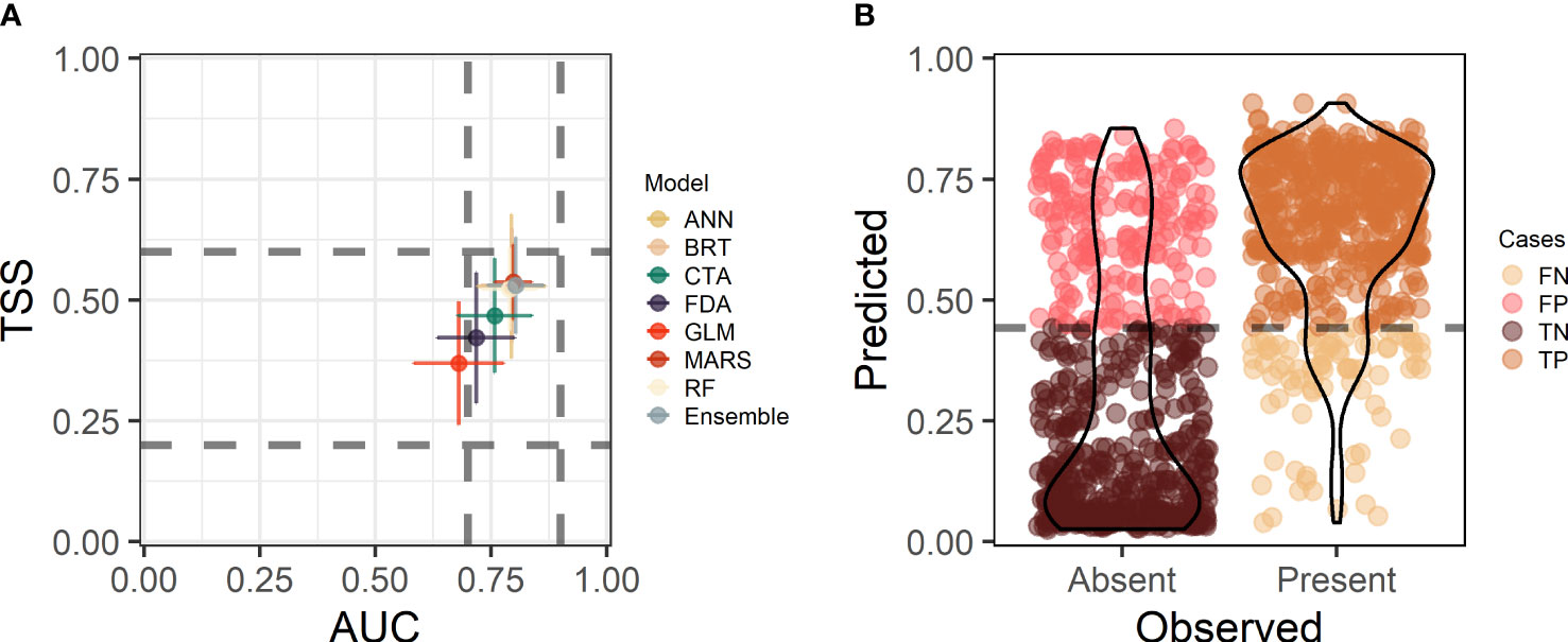
Figure 2 Eelgrass species distribution model performance evaluations: (A) Two evaluation statistics (AUC, TSS) for 7 modeling methods (ANN, BRT, CTA, FDA, GLM, MARS, RF) and the ensemble model. Points are the mean values (± SD) across 5 cross-validation runs. Dashed lines identify thresholds of model performance on each statistic. Below the first horizontal or vertical dashed lines is poor performance, between the first and second lines indicates moderate performance, and above the second horizontal or vertical lines is good performance. (B) Graphical representation of the confusion matrix for the ensemble model. Model predicted (probability) vs. observed (Absent, Present) occurrence of eelgrass. The dashed line is the threshold probability classifying predictions into presence−absence based on the average value across cross-validation runs that maximized the value of the TSS. Colours identify correctly classified (TP, true positive; TN, true negative) vs. misclassified (FP, false positive; FN, false negative) points.
The threshold probability (0.433) chosen to classify ensemble predictions into presence−absence discriminated between observations with minimal false negatives and false positives, but the ensemble model did better to discern seagrass presence than absence (Figure 2B, Table S1). This was reflected by a more pronounced tapering of the kernel density estimate of predicted probabilities above and below this threshold for ‘presence’ records compared to ‘absence’ records (Figure 2B) and a higher model sensitivity (i.e., true positive rate) than specificity (i.e., true negative rate; Table S1). Similar to the ensemble model, all individual modeling methods showed a better ability to predict eelgrass ‘presence’ than ‘absence’ (sensitivity > specificity Table S1). While FDA ranked low on overall performance according to the AUC and TSS, this model also had the highest model sensitivity of all models considered, indicating an improved ability to predict eelgrass ‘presence’. Classification errors were relatively evenly distributed throughout the study area, but errors of omission (i.e., false negatives) were more common within the Mahone Bedrock Shores & Islands and Sheet Harbour Islands coastline classes (Figure S3). Errors of commission (i.e., false positives) were more common within the South Shore Beaches and Eastern Beaches & Drumlins coastline classes (Figure S3).
Coastal-scale distribution of eelgrass and extent of suitable habitat
Model-predicted probabilities of occurrence at locations with validation data showed a bimodal distribution with maxima centered around 0.1 and 0.8 comprising absence and presence records, respectively (Figure 3A). In general, there was a wider range in model uncertainty associated with absence records compared to presence records (Figure 3A). Areas of high probability of eelgrass occurrence as predicted by the ensemble model occurred throughout the spatial domain of the model, but these areas were not evenly distributed along the southeast−northwest oriented Nova Scotia coastline (Figures 3B, 4E). In particular, the highest predicted probabilities were concentrated within the South Shore Beaches area on the southwest tip of the Atlantic coast, the Eastern Shore Beaches and Drumlins area just to the northeast Halifax, East Cape Breton Island Cliffs, and the Bras d’Or Lakes (Figures 3B, 4E). These predictions also tended to be associated with a lower degree of uncertainty as reflected by spatial variation in the standard deviation of ensemble predictions (Figure 3B). Uncertainty in model predictions was influenced mainly by methodological uncertainty (i.e. variation among modeling methods) rather than cross-validation uncertainty (Figure S4). This would suggest variation caused by disagreement among modeling methods rather than geographic non-stationary between the spatially-partitioned subsets of the occurrence data. Some of these areas also had relatively sparse (East Cape Breton, Chedabucto Bay) or no recent eelgrass occurrence records by which to evaluate the model (Bras d’Or Lakes; Figure 1). In the interpretation of the results, consideration should be given to this extrapolation in geographic space (i.e., to areas with relatively few occurrence records) even if predictors were within the range observed in other areas.
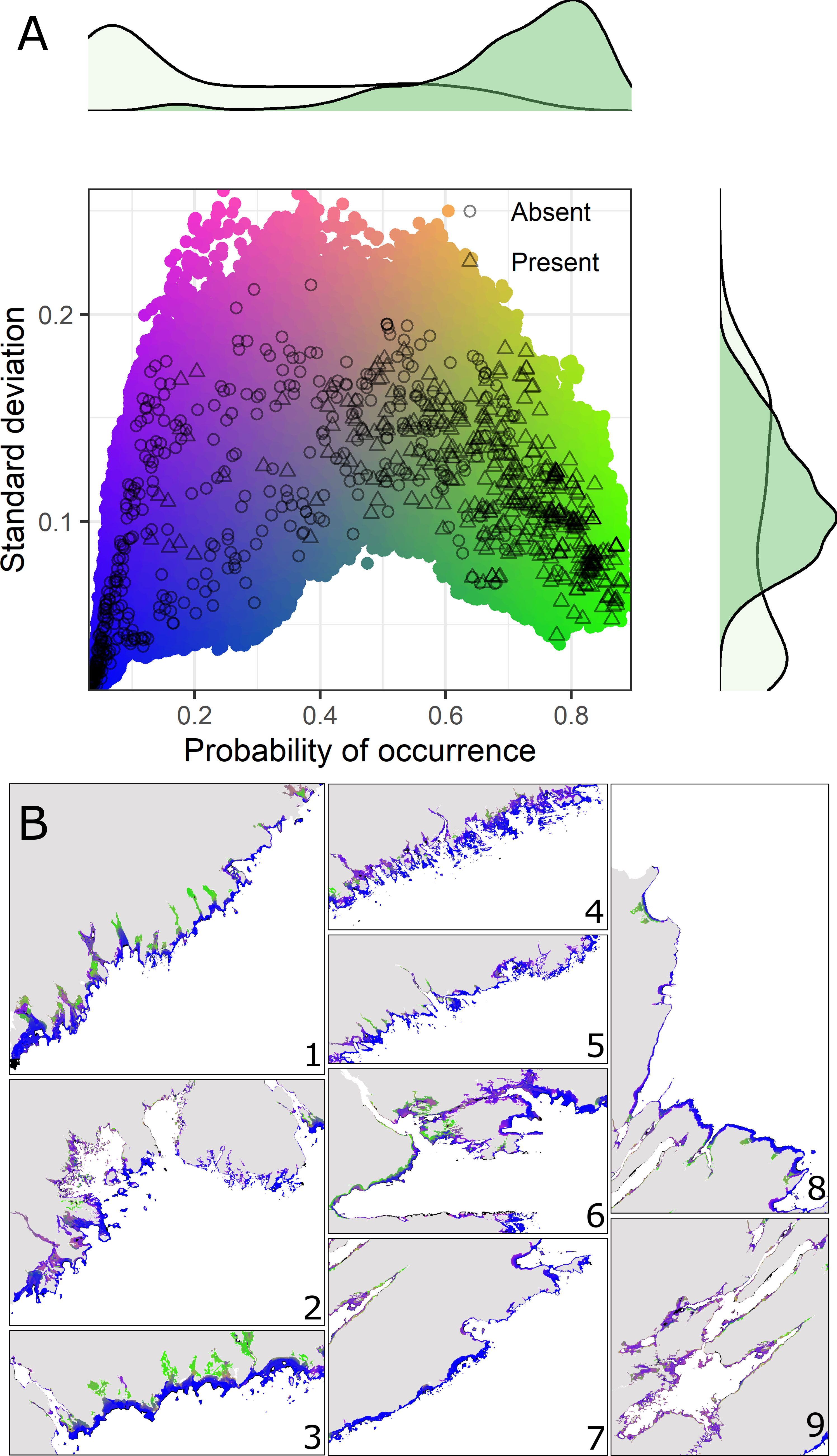
Figure 3 Contemporaneous display of predicted mean probability of occurrence and associated uncertainty (SD) from the ensemble eelgrass model across 5 cross-validation runs. (A) Combined color scale providing interpretation of pixel hue in map insets. Green hues indicate high probability, low uncertainty. Blue hues indicate low probability, low uncertainty. Coloured points identify unique combinations of uncertainty (SD) and probability of occurrence predicted by the ensemble model across the study area extent. Open black symbols indicate predicted values at the locations of eelgrass occurrence records (circle = absence, triangle = presence). Standard deviation of ensemble predictions combines cross-validation uncertainty (i.e., variation across CV runs) and methodological uncertainty (i.e., variation across modeling methods). Marginal density plots show the distribution of predicted probabilities and standard deviation at occurrence record locations (light green = absence, dark green = presence). (B) Model predictions across the study area (35-m nominal resolution) shown with higher detail within particular areas of the coastline (numbered insets) bounded by the extent of nine physiographic coastline classes (see Figure 1 for names and locations of coastline classes corresponding with numbered insets). Areas of extrapolation (i.e., predictors outside range of calibration data) are masked out on maps (black pixels).
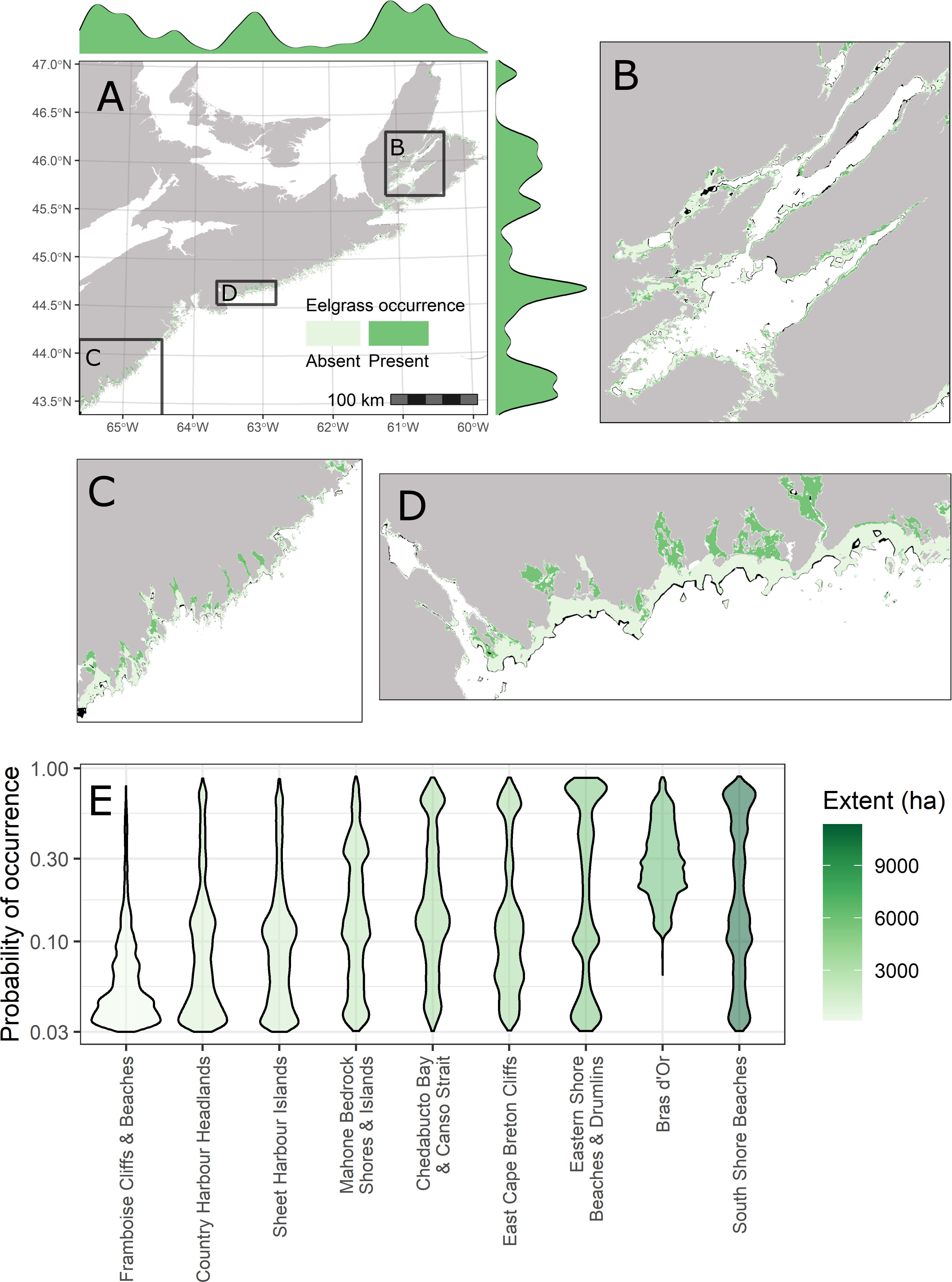
Figure 4 Coastal-scale extent of suitable eelgrass habitat and spatial variation among coastline classes. (A) Binary predictions of the ensemble eelgrass model. Pixel shade indicates the result of reclassifying mean ensemble predicted probability of occurrence based on the average threshold across cross-validation runs that maximized the value of the true skill statistic (TSS). Light green = absent, Dark green = present. Marginal density plots are the kernel density estimates for eelgrass presence predictions across longitudinal (x-axis) and latitudinal gradients (y-axis). Black polygons denote the extents of zoomed in insets shown for the Bras d’Or Lakes (B), South Shore Beaches (C) and Eastern Shore Beaches and Drumlins (D). Areas of model extrapolation are masked out on maps (black pixels). (E) Violin plots with kernel density estimates for probability of occurrence predicted by the ensemble model among physiographic and oceanographic coastline classes (see Figure 1). Deeper shades of green indicate a greater extent (ha) of suitable eelgrass habitat within a coastline class.
Spatial variation in the probability of occurrence also was reflected in the distribution in the predicted extent of suitable eelgrass habitat along the coast (Figure 4). Total extent of eelgrass habitat ranged from 150 ha in the Framboise Cliffs and Beaches area of Cape Breton Island to over 11,000 ha in the South Shores Beaches area of the southwest mainland of Nova Scotia (Figures 4C, E). Extensive eelgrass habitat also was predicted within the Bras d’Or Lakes, East Cape Breton Cliffs, and Eastern Shore Beaches and Drumlins segments of the coastline (Figures 4B, D, E). Areas of the coast with extensive eelgrass habitat tended to be characterized by numerous long and narrow inlets and embayments or large tidal flats (Figures 4A−D). On a coastal scale, the ensemble model predicted a total extent of suitable eelgrass habitat of 38,130 ha, which corresponds to a prevalence of 16.8% over the model spatial domain. We observed substantial overlap of the predicted suitable habitat with coastal EBSAs (Figure 5, Figure S5). Certain EBSAs in particular had a larger proportion of their areal extent (~ 5% − 25%) containing suitable eelgrass habitat. These included Port Joli and Area, Medway Harbour, Cole Harbour – Lawrencetown, Musquodoboit Harbour and Area, Morien Bay, Big Glace Bay, Lingan Bay, Aspy Bay, and Bras d’Or Lakes (Figure 5). Furthermore, compared to a background sample and locations outside EBSA boundaries, model predictions within EBSA boundaries had a higher frequency of predictions that were both high probability and low uncertainty (Figure S5).
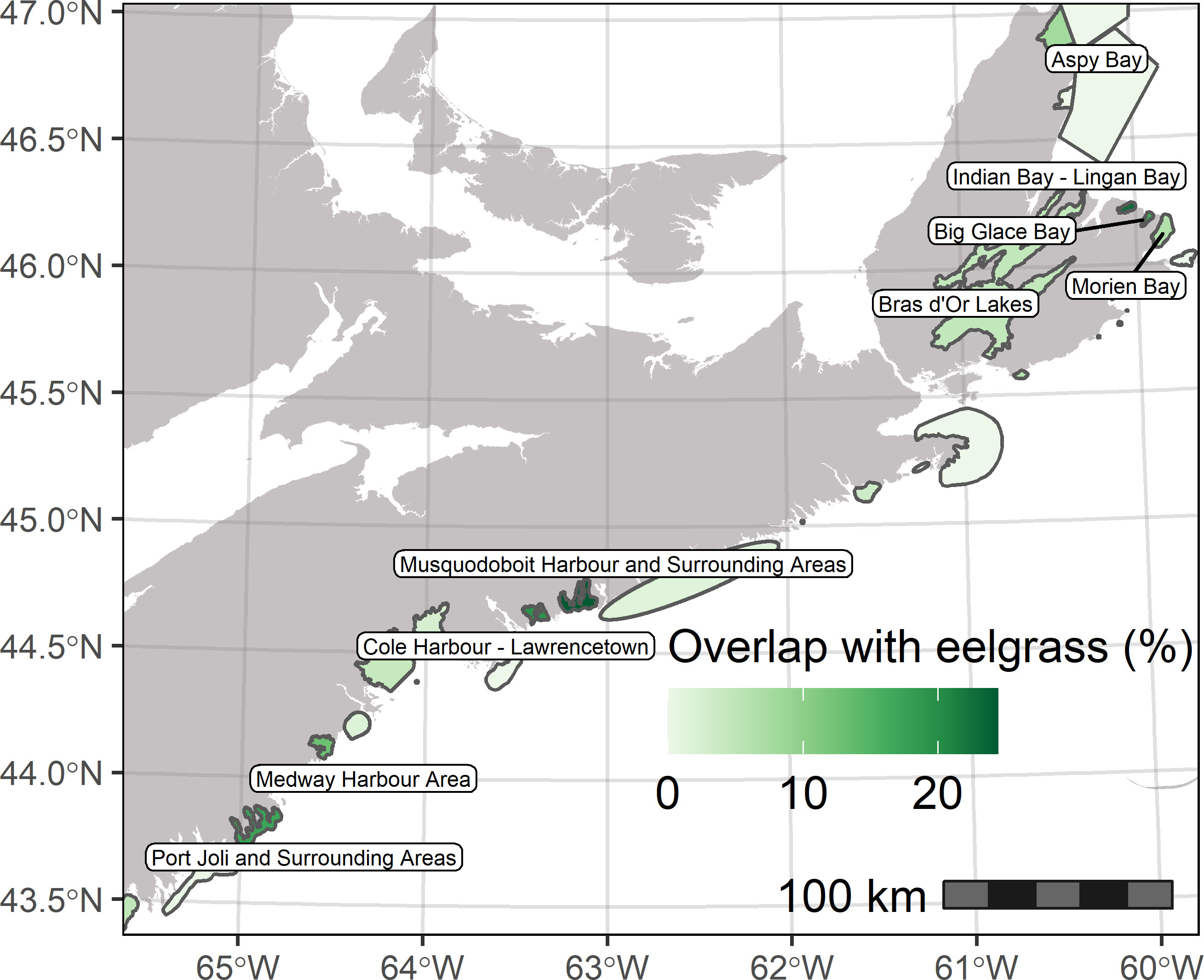
Figure 5 Overlap of predicted suitable eelgrass habitat from ensemble model with coastal Ecologically and Biologically Significant Areas (EBSAs) on the Atlantic coast of Nova Scotia. Colour shading of EBSA polygons denotes degree of overlap with deeper green shades indicating a higher percentage of the EBSA area covered by eelgrass habitat.
Influential environmental predictors
The predicted probability of eelgrass occurrence in the ensemble model was heavily affected by a small number of predictors (Figure 6). Categorical substrate type was the most influential environmental predictor (55.6%), followed by depth (17.7%), and wave exposure (REI; 9.9%) (Figure 6). The bathymetric derivatives (BPI-broad, Slope, and BPI-fine) had minimal importance (collectively 8.8%) in the ensemble model (Figure 6). Substrate type and depth also were consistently important for each individual model and REI was among the top three predictors in 5 of 7 model types (Figure S6). In contrast, slope and BPI consistently ranked low by variable importance among individual models (Figure S6).
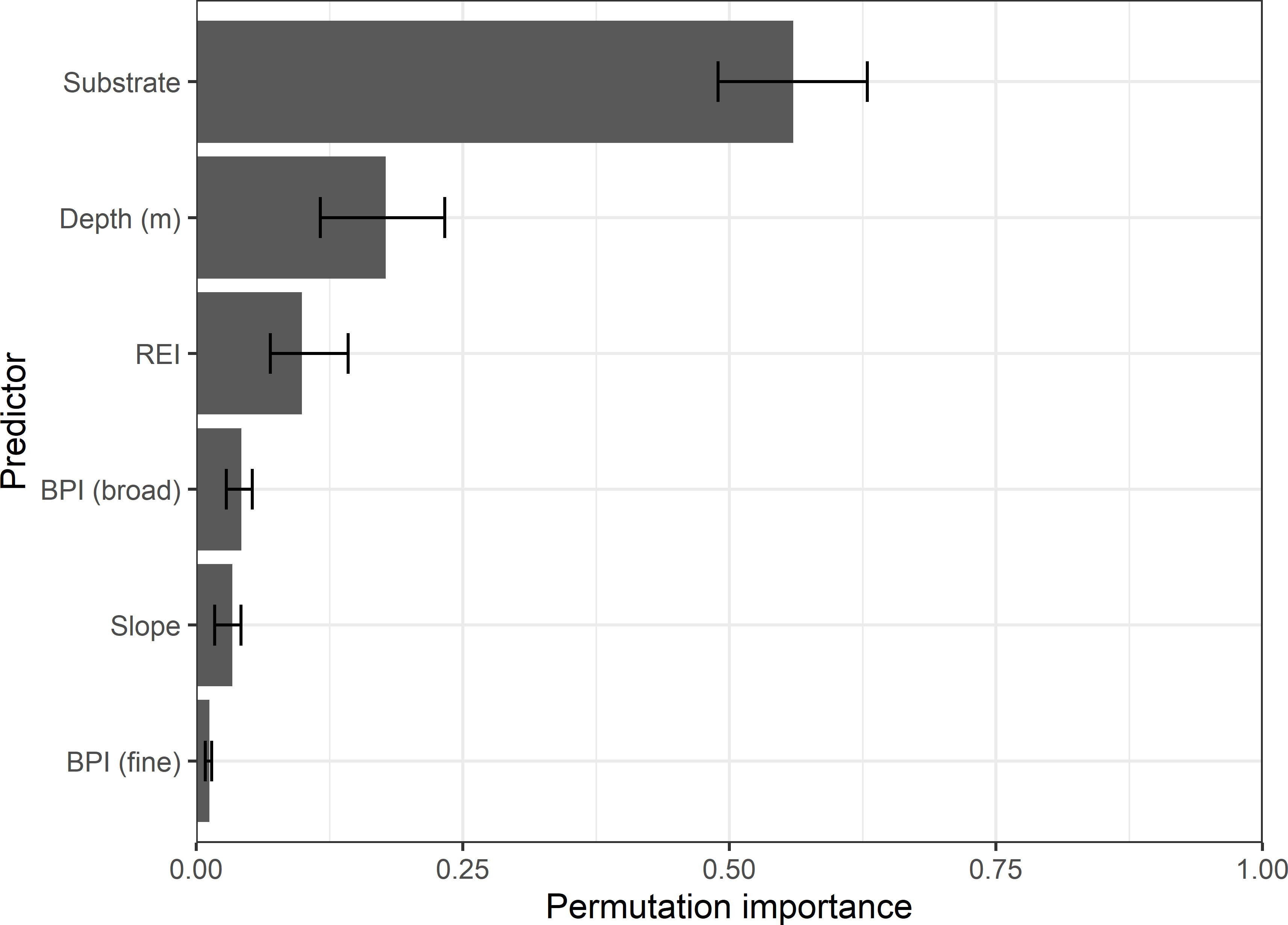
Figure 6 Relative influence of 6 environmental predictors on the probability of eelgrass occurrence predicted by the ensemble model. Bars are the mean permutation importance and errors bars the maximum and minimum importance values across 5-cross validation runs. Predictors include categorical substrate type (muddy, sand & mud, sandy, rocky), depth (m), relative exposure to wind-driven waves (REI; unitless), seabed slope (degrees) and 2 bathymetric position indices (BPI; unitless).
The shape of the response plots varied between the most influential predictors, highlighting different aspects of the ecological niche of eelgrass (Figure 7). For the ensemble model and the top four individual modeling methods (MARS, BRT, ANN, RF), probability of occurrence for eelgrass was highest for sandy substrates or a mix of sand and mud, intermediate for muddy substrates, and relatively lower for predominantly rocky substrates (Figure 7). Probability of occurrence showed a threshold-like response to REI, indicating an upper limit (~ 0.10) on exposure to wind-driven waves (Figure 7). In comparison, the response to depth was more hump-shaped, indicating a higher probability of eelgrass occurrence within the range of 0 – 4 m, and lower probabilities both at deeper depths and shallow depths exposed during low tide (Figure 7). Responses were relatively consistent among the ensemble model and the top four modeling methods (Figure 7). However, the RF model predicted a slightly lowered probability of occurrence at the low end (i.e., more protected) of the wave exposure gradient as well (Figure 7) and RF and BRT showed some indications of overfitting compared to ANN, MARS, and the ensemble.
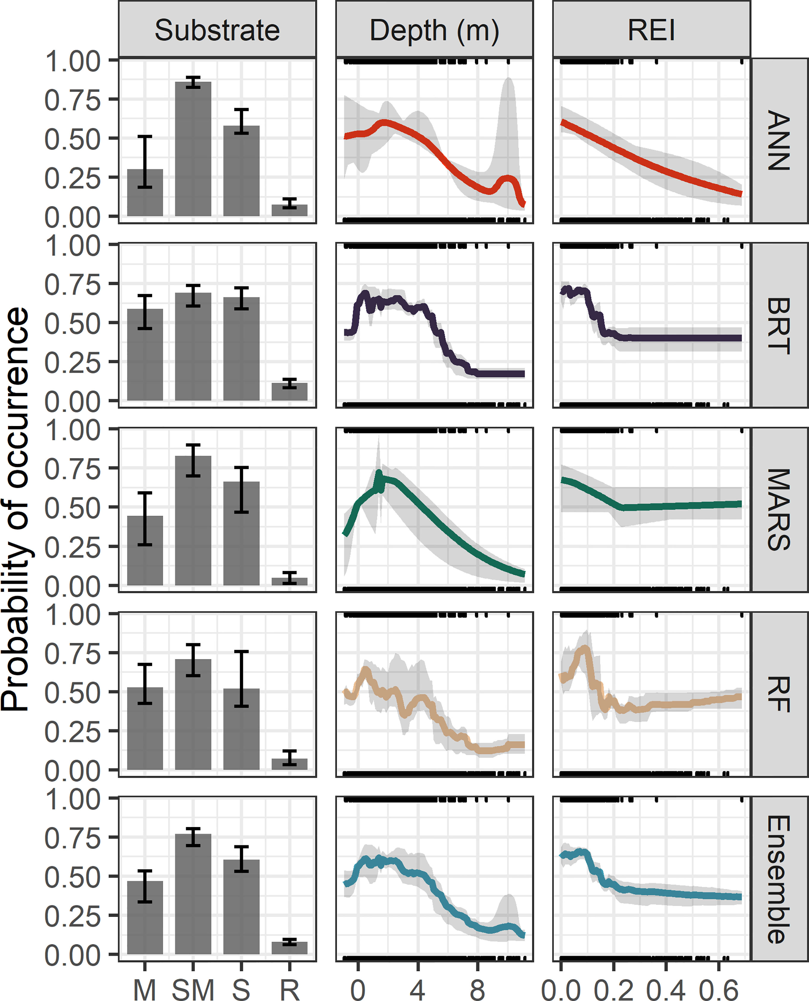
Figure 7 Response plots for the 3 most influential predictors of eelgrass occurrence in the top-performing individual species distribution modeling methods (MARS, BRT, ANN, RF) and the ensemble model. Predictors include categorical substrate type (muddy – M, sand & mud – SM, sandy – S, rocky – R), depth (m), and a relative exposure index to wind-driven waves (REI, unitless). Bars and lines show the mean probability of occurrence predicted by each model method over 5 cross-validation runs across the range of each predictor with other variables held at their median value. Error bars and shaded regions indicate the maximum and minimum value across the 5 CV runs. Rug plots show the marginal distributions of predictors in the calibration data for records of eelgrass presence (top) and absence (bottom).
Discussion
With our ensemble model, we identified almost 40,000 ha of suitable eelgrass habitat at a high spatial resolution on a coastal scale, filling substantial observational gaps in the known occurrence of eelgrass while highlighting areas of coastline with extensive habitat overlapping with areas prioritized for protection. Our ensemble model for eelgrass demonstrated high sensitivity and moderate predictive performance with respect to threshold-dependent (TSS) and threshold-independent (AUC) evaluation metrics, offering moderate improvement on AUC and sensitivity compared to the best-performing individual SDM methods. Our results are consistent with previous seagrass modeling studies that found improvement of ensemble models on various performance metrics and often higher sensitivity compared to individual models (Downie et al., 2013; Chefaoui et al., 2016; Chefaoui et al., 2017; Chefaoui et al., 2018). When modeling distributions for species prioritized for conservation, increased sensitivity and even modest improvements in overall performance are particularly beneficial given that greater value is placed on correct predictions of species presence and predictions may guide the location of protected area boundaries. Furthermore, model comparisons of SDMs for seagrasses and other vascular plants have shown ensemble models often outperform untuned individual models under external cross-validation with independent data and yield similar or superior performance to even well-tuned models (Folmer et al., 2016; Hao et al., 2020). Consequently, by reducing the contingency of model performance and transferability on the choice of model and tuning parameters, we contend that the ensemble approach is preferable for guiding conservation and local management decisions.
In our model, the averaging of predictions by the ensemble appeared to smooth out some of the known overfitting tendencies of the machine-learning algorithms (Figure 6), which may improve model transferability. While increasingly complex models often improve fit by better capturing non-linear behaviour, there is the potential risk of overfitting the data leading to poor model transfer in new areas and novel conditions (Gregr et al., 2019; Hao et al., 2020). We observed that machine-learning (BRT, RF, ANN) and regression methods (MARS) capable of fitting more complex non-linear responses yielded the most accurate predictions among individual models, consistent with previous comparisons of model performance made between SDMs developed for Z. marina in the Wadden Sea (Valle et al., 2013), other marine macrophytes (Chefaoui et al., 2016; Chefaoui et al., 2017; Chefaoui et al., 2018; Goldsmit et al., 2021), and for freshwater (Grenouillet et al., 2011; Guo et al., 2015), and terrestrial species (Elith et al., 2006). However, contrary to our expectation, with the exception of the GLM, overall performance did not vary widely among modeling methods. This may reflect the dominant influence of a small number of predictors, namely substrate type, on the species-environment response and therefore classification success for eelgrass occurrence. Although evaluation against an independent dataset would be required to fully assess the suitability of our ensemble model for extrapolation tasks (e.g., Folmer et al., 2016), convergence among model predictions should increase confidence in management decisions when extrapolating outside model training areas.
Our ensemble SDM for eelgrass fit within a subset of its biogeographic range demonstrated comparable predictive performance to previous single-technique SDMs developed in other regions within the biogeographic range of Zostera marina at a similar nominal resolution (Bekkby et al., 2008; Downie et al., 2013; Schubert et al., 2015; Bobsien et al., 2021). However, ensemble and single-model SDMs fit over the entire species biogeographic range of marine macrophytes or across a broader latitudinal gradient have typically shown higher predictive performance (AUC > 0.9, TSS > 0.7) for seagrasses (Valle et al., 2014; Chefaoui et al., 2016; Chefaoui et al., 2017; Chefaoui et al., 2018; Wilson and Lotze, 2019; Chefaoui et al., 2021; Hu et al., 2021), kelps (Assis et al., 2018; Wilson et al., 2019b; Goldsmit et al., 2021), and mangroves (Record et al., 2013). These range-wide models mainly employ climatic predictors at a coarser resolution (e.g., ~ 5 arc min), which may explain their improved fit given that marine species occupy geographic ranges close to their thermal limits (Sunday et al., 2012), potentially yielding stronger correlations with species occurrence across their temperature range at a coarse scale. Comparative studies also have shown that SDMs with high spatial resolution (< 1 km), while gaining in granularity, may sacrifice a degree of predictive accuracy (Lowen et al., 2016; Farashi and Alizadeh-Noughani, 2018), accounting for some of the discrepancy in performance between fine-scale within-range models relative to more coarsely resolved range-wide models. In addition, range-wide SDMs for seagrasses have typically been fit for species with smaller geographic ranges and narrower environmental tolerances (e.g., Posidonia oceanica, Zostera noltei, Thalassia hemprichii, Cymodocea nodosa), which tend to be more accurately modelled using SDM techniques (Segurado and Araújo, 2004; Grenouillet et al., 2011) compared to widely distributed species and habitat generalists such as Z. marina. Even still, regionally tailored models may be more appropriate for widely distributed species if local adaptation occurs among subpopulations or spatial inconsistencies in species-environment relationships exist (Osborne and Suárez-Seoane, 2002; Stockwell and Peterson, 2002; Lowen et al., 2019).
The choice of model scale (within-range vs. range-wide) should be informed to a large degree by the modeling objectives and intended applications as they are best suited for different purposes based on a trade-off between spatial resolution and extent. Whereas, models covering the entire biogeographic range calibrated with coarser grain climatic predictors may reveal tolerance limits and permit projections of past (Chefaoui et al., 2017; Assis et al., 2018) or future species distributions (Wilson and Lotze, 2019; Chefaoui et al., 2021), models fit within a species’ range can uncover more subtle niche preferences and local adaptation (Nephin et al., 2020), corresponding to more fine-scale and complex forcing that reflect habitat suitability closer to the scale of habitat patch sizes. These more nuanced relationships deteriorate at larger spatial scales (Record et al., 2013) and the relative influence of environmental predictors may change (Nyström Sandman et al., 2013), yet such fine-grain, regional distribution patterns are critical to local conservation planning and habitat management. For example, a presence-only SDM developed by Wilson and Lotze (2019) over the latitudinal range of eelgrass in the Northwest Atlantic predicted a contraction of the southern range and expansion of suitable habitat in Arctic and subarctic regions by end-century. Contrary to our results, the range-wide model, influenced heavily by sea surface temperature, predicted little differentiation in habitat suitability along the Atlantic coast of Nova Scotia. Both predictions provide useful information to conservation planners, but at fundamentally different spatial scales. Range-wide models highlight large-scale distributional changes associated with changing climatic conditions, particularly at range edges, but the lower resolution may lead to a scale mismatch that hinders local decision-making related to targeted conservation that is better informed by high resolution within-range models.
Trade-offs between resolution and extent also constrain remote sensing methods for mapping seagrass beds in turbid coastal waters. While seagrass habitats have been mapped on a regional scale using multispectral satellite imagery (e.g., Landsat, Sentinel-2), these applications have generally been limited to optically clear, often tropical waters (e.g., Torres-Pulliza et al., 2013; Traganos et al., 2018). In the optically complex coastal waters along the Atlantic coast of Nova Scotia, image-based classification of multispectral imagery has been used with mixed success to map eelgrass and SAV. In areas with high water clarity, Wilson et al. (2019a) accurately classified eelgrass, seaweeds, and bare substrate to 8 m. However, in areas with more optically active components in the water column, eelgrass could not be distinguished from other SAV with similar spectral profiles and reliable classification was reduced to depths as shallow as 2 m or was precluded entirely (Wilson et al., 2019a; Wilson et al., 2020). Classification success was also reduced for sparse or patchy vegetation and on muddy substrates relative to continuous beds on sandy substrates (Wilson et al., 2020). Our results highlight that suitable eelgrass habitat can occur on muddy substrates and below 2 m depth suggesting that satellite-based sensors could overlook significant areas of suitable eelgrass habitat in regions with optically complex nearshore waters. In particular, eelgrass beds in deeper waters are often found in cooler areas of higher wave exposure, which are generally more productive and resilient compared to beds in warm, shallow areas subject to temperature and light stress (Krumhansl et al., 2021), exhibit different life-history strategies (Vercaemer et al., 2021), and enhance benthic secondary production (Wong, 2018). While hyperspectral sensors and acoustic mapping methods have improved capability to detect eelgrass in deeper, more turbid waters, or patchy beds, these techniques are generally limited in spatial extent of application (e.g., Barrell et al., 2015; Dierssen et al., 2019). We contend that remote sensing and SDM methods offer complementarity if used in tandem given the common requirement for ground-truth data and the ability of each to resolve different aspects of distribution. Just as ensemble SDMs are designed to address methodological uncertainty, so too could predictions of remote sensing and SDM techniques be combined. Where significant data gaps exist, the predictive power of SDMs can be leveraged to identify and prioritize areas for more in-depth characterization, mapping, and monitoring using remote sensing tools.
Using the coastal-scale predictions of our ensemble model, we identified several areas of the coastline with extensive area of suitable eelgrass habitat, which can inform regional conservation priority-setting. Interestingly, many of the areas identified by the SDM are also designated as coastal EBSAs based on scientific expert opinion with consideration for the presence of eelgrass (Doherty and Horsman, 2007; Hastings et al., 2014), yet only a few of these identified areas have been extensively mapped for eelgrass distribution (Bras d’Or: Vandermeulen, 2016, Port Joli: Vandermeulen, 2017; Wilson et al., 2019a; Petpeswick Inlet & Musquodoboit Harbour: NS Department of Natural Resources unpubl.). These coastal EBSAs provide the basis for nearshore conservation network planning in the region (King et al., 2021), underscoring the value of scalable approaches such as SDMs for validating expert opinion.
Policy and management strategies informed by SDMs should explicitly consider prediction uncertainty as well, yet estimates of model uncertainty are rarely provided in marine-based SDM studies (Robinson et al., 2017). In our study, we explicitly mapped probability of eelgrass occurrence alongside associated uncertainty, which can facilitate conservation planning and other spatial habitat management strategies (e.g. MSP) while acknowledging model limitations. For example, areas of high probability and low uncertainty should be prioritized for protection and risk management, while areas of high probability and high uncertainty will benefit from further directed investigation and more detailed mapping with appropriate remote sensing methods. The high probability of eelgrass and low uncertainty predicted by our ensemble model within certain EBSA boundaries confirms expert opinion of their ecological significance based on the presence of biogenic habitat within the EBSA, while also providing a much more detailed assessment of within-EBSA distribution. This approach provides further justification for additional risk-management strategies in those areas. Consideration of spatial variation in model classification errors can also guide habitat management activities. For example, we identified broader sections of the coastline in which model errors of commission (i.e., false positives) were more common, which have been suggested by Bittner et al. (2020) as candidate regions for restoration efforts. The identification of influential environmental predictors and their marginal effects by distribution models such as ours also provides relevant information about suitable habitat features that could further guide such restoration activities. However, false positive areas will require in-depth evaluation of other aspects of the supporting environment that may affect habitat suitability (e.g., light, temperature, water quality).
We identified substrate type, water depth, and relative wave exposure as the most important variables in the ensemble SDM determining habitat suitability for eelgrass with substrate being particularly influential. The essential requirement of seagrass for soft substrate is self-evident, but our model showed the probability of eelgrass occurrence was also lower on fine-grain muddy substrates compared to more sandy sediments. Fine grain sediments are often enriched in organic matter content (Fonseca and Bell, 1998; Wicks et al., 2009; Krause-Jensen et al., 2011) with concomitant increases in hydrogen sulfide (Pérez et al., 2007; Krause-Jensen et al., 2011), a well-known phytotoxin to eelgrass and other SAV (Goodman et al., 1995; Koch, 2001; Pérez et al., 2007) that becomes problematic under hypoxic conditions linked to environmental stress or poor water quality (Koch et al., 2022). Fine sediments high in organic content are more common in quiescent areas of lower current velocities and wave exposure (Fonseca and Bell, 1998; Koch, 2001; Krumhansl et al., 2021), but SAV is also subject to diffusive boundary layer constraints in areas of lower water motion (Koch, 2001). While we found evidence of reduced probability of eelgrass occurrence at more protected locations (RF model), we observed a more pronounced threshold-like decrease in habitat suitability at the upper end of the wave exposure gradient, consistent with wave-induced disturbance leading to reduced cover and bed continuity of seagrass habitats (Fonseca and Bell, 1998). Physical forces such as wave exposure also determine the minimum depth limit of SAV, while maximum depth limits are constrained by light availability (Koch, 2001; De Boer, 2007; Krause-Jensen et al., 2011). Our ensemble model predicted a relatively unimodal probability distribution across depth (highest between 0 m – 4 m) consistent with these constraints and previously published depth limits for Z. marina in Danish waters (mean of 3.5 m; Krause-Jensen et al., 2011).
The importance of depth and wave exposure likely also reflect strong correlations with other physical gradients more proximately related to eelgrass distribution, abundance, productivity, and resilience. Wave exposure and to a lesser extent depth have been correlated with several emergent properties of eelgrass ecosystems from physiological to landscape scales, but these biological responses likely are driven mainly by direct effects of temperature and light rather than explicitly by water motion and depth (Krumhansl et al., 2021). Deeper eelgrass beds in wave exposed areas experience lower light attenuation, cooler mean temperature conditions, and reduced temperature variability and extremes relative to shallow protected beds (Krumhansl et al., 2020; Wong and Dowd, 2021), because of increased flushing and water exchange. Eelgrass shows negative short- and long-term responses to both chronic and episodic light reduction (Lefcheck et al., 2017; Wong et al., 2020; Wong et al., 2021), which can exacerbate effects of temperature stress (Lefcheck et al., 2017; Wong et al., 2020). Temperature stress has been linked to reduced seasonal growth and productivity of eelgrass (Lee et al., 2005; Wong et al., 2013), recent estuary-scale declines in abundance (Lefcheck et al., 2017), and forecasted distribution changes (Wilson and Lotze, 2019). Despite the importance of light and temperature conditions to the status of eelgrass ecosystems, and the preference to include predictors in SDMs with more direct linkages to ecological functioning, proxies such as depth and REI can actually have more predictive power compared to more proximate predictors in fine-grain within-range SDMs for nearshore species (Bekkby et al., 2008; Gregr et al., 2019; Nephin et al., 2020), perhaps related to the difficulty of modeling the complex and highly variable physical processes themselves in the nearshore at a high resolution. Environmental variability over shorter times scales (i.e., sub-seasonal processes) are key determinants of eelgrass productivity and resilience (Krumhansl et al., 2021; Wong and Dowd, 2021), but temperature layers derived from down-scaling of commonly available regional and global oceanographic models most often do not appropriately resolve such short-term physical processes that are important at local scales. Therefore, the development of regional circulation models that better capture these short-term, small spatial scale dynamics (e.g., Feng et al., 2022) will be necessary to extend our SDM to make regional climate projections at the high spatial resolution required to build climate resilience into conservation networks.
Conclusion
Achieving ambitious conservation and restoration targets for seagrasses and other habitat-forming macrophytes will require the rapid identification of suitable habitat at a spatial scale and resolution relevant for regional decision-makers and restoration projects. Aggressive protection is necessary, but is likely not sufficient to ensure global recovery of seagrass ecosystems (Buelow et al., 2022). Recovery of seagrass ecosystems will require a portfolio of target conservation and restoration work. The success of restoration projects is contingent on large-scale transplantation (van Katwijk et al., 2016), exacerbating the need to delineate large areas of suitable habitat. The long-term viability of protected areas and restored habitats will also hinge on the identification and management of local stressors in these areas of high suitability. We demonstrated how ensemble species distribution models can provide regional-scale predictions of the distribution and extent of suitable habitat for SAV at a relatively fine spatial resolution and with high sensitivity, characterize the relevant environmental features of habitat suitability, and support uncertainty estimation. This approach provides complementary tools to inform conservation planning, restoration, and other habitat management strategies in coastal environments that challenge the limits of remote sensing applications. Furthermore, the insights provided by ensemble SDMs can also facilitate marine spatial planning processes, emergency response planning, evaluation of carbon sequestration and storage by SAV, and habitat-specific assessments of anthropogenic and cumulative impacts. With the emergence of blue carbon offset crediting (Kuwae et al., 2022) and more ambitious post-2020 biodiversity agreement under the Convention on Biological Diversity (CBD Secretariat, 2021), the more balanced approach provided by ensemble modeling techniques that integrate information from numerous models in their spatial predictions, characterize species-environment relationships, and allow concurrent assessment and display of probability of occurrence and uncertainty will become increasingly pertinent to support the accelerated protection and restoration of shallow nearshore ecosystems and the pivotal functions and services they provide.
Data availability statement
The raw data supporting the conclusions of this article will be made available by the authors, without undue reservation.
Author contributions
JO’B created the sampling design, collected the data, designed and performed the analysis, and led the manuscript writing. MW conceived of the study, created the sampling design, collected the data, designed the analysis, and contributed to the manuscript text. RS conceived of the study, created the sampling design, designed the analysis, and contributed to the manuscript text. All authors contributed to the article and approved the submitted version.
Funding
This research was funded by Fisheries and Oceans Canada (MW).
Acknowledgments
We are grateful to Betty Roethlisberger, Benedikte Vercaemer, Shawn Roach, Stephanie Robertson-Kempton, and Javier Guijarro-Sabaniel for their assistance in the field with drop camera surveys. Adam Kennedy and Smaknis Maritime Safety & Security Inc. supported surveys through provision and operation of survey vessels. Stephanie Robertson-Kempton performed grain size analysis of sediment samples collected during camera surveys.
Conflict of interest
The authors declare that the research was conducted in the absence of any commercial or financial relationships that could be construed as a potential conflict of interest.
Publisher’s note
All claims expressed in this article are solely those of the authors and do not necessarily represent those of their affiliated organizations, or those of the publisher, the editors and the reviewers. Any product that may be evaluated in this article, or claim that may be made by its manufacturer, is not guaranteed or endorsed by the publisher.
Supplementary material
The Supplementary Material for this article can be found online at: https://www.frontiersin.org/articles/10.3389/fmars.2022.988858/full#supplementary-material
Supplementary Data Sheet 1 | Supplementary tables and figures.
References
Araújo M. B., New M. (2007). Ensemble forecasting of species distributions. Trends Ecol. Evol. 22, 42–47. doi: 10.1016/j.tree.2006.09.010
Assis J., Araújo M. B., Serrão E. A. (2018). Projected climate changes threaten ancient refugia of kelp forests in the north Atlantic. Glob Chang Biol. 24, e55–e66. doi: 10.1111/gcb.13818
Barbier E., Hacker S., Kennedy C., Koch E., Stier A., Silliman B. (2011). The value of estuarine and coastal ecosystem services. Ecol. Monogr. 81 (2), 169–193. doi: 10.1890/10-1510.1
Barrell J., Grant J., Hanson A., Mahoney M. (2015). Evaluating the complementarity of acoustic and satellite remote sensing for seagrass landscape mapping. Int. J. Remote Sens 36, 4069–4094. doi: 10.1080/01431161.2015.1076208
Beazley L., Kenchington E., Murillo F. J., Brickman D., Wang Z., Davies A. J., et al. (2021). Climate change winner in the deep sea? predicting the impacts of climate change on the distribution of the glass sponge Vazella pourtalesii. Mar. Ecol. Prog. Ser. 657, 1–23. doi: 10.3354/meps13566
Bekkby T., Rinde E., Erikstad L., Bakkestuen V., Longva O., Christensen O., et al. (2008). Spatial probability modelling of eelgrass (Zostera marina) distribution on the west coast of Norway. ICES J. Mar. Sci. 65, 1093–1101. doi: 10.1093/icesjms/fsn095
Bittner R. E., Roesler E. L., Barnes M. A. (2020). Using species distribution models to guide seagrass management. Estuar. Coast. Shelf Sci. 240, 106790. doi: 10.1016/j.ecss.2020.106790
Blok S. E., Olesen B., Krause-Jensen D. (2018). Life history events of eelgrass Zostera marina l. populations across gradients of latitude and temperature. Mar. Ecol. Prog. Ser. 590, 79–93. doi: 10.3354/meps12479
Bobsien I. C., Hukriede W., Schlamkow C., Friedland R., Dreier N., Schubert P. R., et al. (2021). Modeling eelgrass spatial response to nutrient abatement measures in a changing climate. Ambio 50, 400–412. doi: 10.1007/s13280-020-01364-2
Buelow C., Connolly R., Turschwell M., Adame M., Ahmadia G., Andradi-Brown D., et al. (2022). Ambitious global targets for mangrove and seagrass recovery. Curr. Biol 32, 1641–1649.e3. doi: 10.1016/j.cub.2022.02.013
Bundy A., Themelis D., Sperl J., Den Heyer N. (2014). Inshore Scotian Shelf ecosystem overview report: Status trends. DFO. Can. Sci. Advis. Sec. Res. Doc. 2014/065, xii +213.
Cavanaugh K. C., Bell T., Costa M., Eddy N. E., Gendall L., Gleason M. G., et al. (2021). A review of the opportunities and challenges for using remote sensing for management of surface-canopy forming kelps. Front. Mar. Sci. 8. doi: 10.3389/fmars.2021.753531
CBD (2022). First Draft of the Post-2020 Global Biodiversity Framework, CBD/WG2020/3/3. .([pdf] Convention on Biological Diversity). Available at: https://www.cbd.int/doc/c/abb5/591f/2e46096d3f0330b08ce87a45/wg2020-03-03-en.pdf (Accessed 6 June 2022).
Cebrian J. (1999). Patterns in the fate of production in plant communities. Am. Nat. 154, 449–468. doi: 10.1086/303244
Chefaoui R. M., Assis J., Duarte C. M., Serrão E. A. (2016). Large-Scale prediction of seagrass distribution integrating landscape metrics and environmental factors: The case of Cymodocea nodosa (Mediterranean–Atlantic). Estuaries Coasts 39, 123–137. doi: 10.1007/s12237-015-9966-y
Chefaoui R. M., Duarte C. M., Serrão E. A. (2017). Paleoclimatic conditions in the Mediterranean explain genetic diversity of Posidonia oceanica seagrass meadows. Sci. Data 7, 2732. doi: 10.1038/s41598-017-03006-2
Chefaoui R. M., Duarte C. M., Serrão E. A. (2018). Dramatic loss of seagrass habitat under projected climate change in the Mediterranean Sea. Glob Chang Biol. 24, 4919–4928. doi: 10.1111/gcb.14401
Chefaoui R. M., Duarte C. M., Tavares A. I., Frade D. G., Sidi Cheikh M. A., Abdoull Ba M., et al. (2021). Predicted regime shift in the seagrass ecosystem of the Gulf of Arguin driven by climate change. Glob Ecol. Conserv. 32, e01890. doi: 10.1016/j.gecco.2021.e01890
De Boer W. F. (2007). Seagrass-sediment interactions, positive feedbacks and critical thresholds for occurrence: A review. Hydrobiologia 591, 5–24. doi: 10.1007/s10750-007-0780-9
Dewsbury B. M., Bhat M., Fourqurean J. W. (2016). A review of seagrass economic valuations: Gaps and progress in valuation approaches. Ecosyst. Serv. 18, 68–77. doi: 10.1016/j.ecoser.2016.02.010
DFO (2009). Does eelgrass (Zostera marina) meet the criteria as an ecologically significant species? Can. Sci. Advi. Secretariat Sci. Advisory Rep. 2009/018, 1–11.
DFO (2012). Definitions of harmful alteration, disruption or destruction (HADD) of habitat provided by eelgrass (Zostera marina). Can. Sci. Advis. Secr. Sci. Advis. Rep. 2011/058, 1–21.
DFO (2018). Design strategies for a network of marine protected areas in the Scotian Shelf Bioregion. DFO Can. Sci. Advis. Sec Sci. Advis Rep. 2018/006. 1–23
DFO (2022). Data from: A substrate classification for the inshore Scotian Shelf and Bay of Fundy, Maritimes Region. Government of Canada Open Data Portal. https://open.canada.ca/data/en/dataset/f2c493e4-ceaa-11eb-be59-1860247f53e3
Dierssen H. M., Bostrom K. J., Chlus A., Hammerstrom K., Thompson D. R., Lee Z. (2019). Pushing the limits of seagrass remote sensing in the turbid waters of Elkhorn Slough, California. Remote Sens 11, 13–15. doi: 10.3390/rs11141664
Doherty P., Horsman T. (2007). Ecologically and biologically significant areas of the Scotian shelf and environs: A compilation of scientific expert opinion. Can. Tech. Rep. Fish. Aquat. Sci. 277457 + xii
Dormann C. F., Purschke O., Márquez J. R. G., Lautenbach S., Schröder B. (2008). Components of uncertainty in species distribution analysis: A case study of the great grey shrike. Ecology 89, 3371–3386. doi: 10.1890/07-1772.1
Downie A. L., Von Numers M., Boström C. (2013). Influence of model selection on the predicted distribution of the seagrass Zostera marina. Estuar. Coast. Shelf Sci. 121–122, 8–19. doi: 10.1016/j.ecss.2012.12.020
Dunic J. C., Brown C. J., Connolly R. M., Turschwell M. P., Côté I. M. (2021). Long-term declines and recovery of meadow area across the world’s seagrass bioregions. Glob Chang Biol. 27, 4096–4109. doi: 10.1111/gcb.15684
Eger A., Marzinelli E., Baes R., Blain C., Blamey L., Carnell P. (2021). The economic value of fisheries, blue carbon, and nutrient cycling in global marine forest. EcoEvoRxiv. Available at: https://ecoevorxiv.org/n7kjs/
Eger A. M., Marzinelli E., Gribben P., Johnson C. R., Layton C., Steinberg P. D., et al. (2020). Playing to the positives: Using synergies to enhance kelp forest restoration. Front. Mar. Sci. 7, 1–15. doi: 10.3389/fmars.2020.00544
Elith J., Ferrier S., Huettmann F., Leathwick J. (2005). The evaluation strip: A new and robust method for plotting predicted responses from species distribution models. Ecol. Modell 186, 280–289. doi: 10.1016/j.ecolmodel.2004.12.007
Elith J., Graham C. H. (2009). Do they? how do they? WHY do they differ? on finding reasons for differing performances of species distribution models. Ecography (Cop) 32, 66–77. doi: 10.1111/j.1600-0587.2008.05505.x
Elith J., Graham C. H., Anderson R. P., Dudík M., Ferrier S., Guisan A., et al. (2006). Novel methods improve prediction of species’ distributions from occurrence data. J Ecography 29 129–151. doi: 10.1111/j.2006.0906-7590.04596.x
Environment and Climate Change Canada (2020) Canadian Environmental sustainability indicators. In: Eelgrass in Canada. Available at: www.canada.ca/en/environment-climate-change/services/environmental-indicators/eelgrass-canada.html (Accessed 31 January 2022).
Farashi A., Alizadeh-Noughani M. (2018). Effects of models and spatial resolutions on the species distribution model performance. Model. Earth Syst. Environ. 4, 263–268. doi: 10.1007/s40808-018-0422-4
Feng T., Stanley R. R. E., Wu Y., Kenchington E., Xu J., Horne E. (2022). A high-resolution 3-d circulation model in a complex archipelago on the coastal Scotian Shelf. J. Geophys Res. Ocean 127, 1–23. doi: 10.1029/2021JC017791
Folmer E. O., van Beusekom J. E. E., Dolch T., Gräwe U., van Katwijk M. M., Kolbe K., et al. (2016). Consensus forecasting of intertidal seagrass habitat in the Wadden Sea. J. Appl. Ecol. 53, 1800–1813. doi: 10.1111/1365-2664.12681
Fonseca M. S., Bell S. S. (1998). Influence of physical setting on seagrass landscapes. Mar. Ecol. Prog. Ser. 171, 109–121. doi: 10.3354/meps171109
Goldberg L., Lagomasino D., Thomas N., Fatoyinbo T. (2020). Global declines in human-driven mangrove loss. Glob Chang Biol. 26, 5844–5855. doi: 10.1111/gcb.15275
Goldsmit J., Schlegel R. W., Filbee-Dexter K., MacGregor K. A., Johnson L. E., Mundy C. J., et al. (2021). Kelp in the Eastern Canadian Arctic: Current and future predictions of habitat suitability and cover. Front. Mar. Sci. 18, 742209. doi: 10.3389/fmars.2021.742209
Goodman J. L., Moore K. A., Dennison W. C. (1995). Photosynthetic responses of eelgrass (Zostera marina l.) to light and sediment sulfide in a shallow barrier island lagoon. Aquat Bot. 50, 37–47. doi: 10.1016/0304-3770(94)00444-Q
Greenlaw M. E., Gromack A. G., Basquill S. P., Mackinnon D. S., Lynds J. A., Taylor R. B., et al. (2012). A physiographic coastline classification of the Scotian Shelf Bioregion and environs: The Nova Scotia coastline and the New Brunswick Fundy shore. Can. Sci. Advis Secr 2012, 43.
Gregr E. J., Palacios D. M., Thompson A., Chan K. M. A. (2019). Why less complexity produces better forecasts: an independent data evaluation of kelp habitat models. Ecography (Cop) 42, 428–443. doi: 10.1111/ecog.03470
Grenouillet G., Buisson L., Casajus N., Lek S. (2011). Ensemble modelling of species distribution: The effects of geographical and environmental ranges. Ecography (Cop) 34, 9–17. doi: 10.1111/j.1600-0587.2010.06152.x
Guisan A., Zimmermann N. E. (2000). Predictive habitat distribution models in ecology. Ecol. Modell 135, 147–186. doi: 10.1016/S0304-3800(00)00354-9
Gumusay M. U., Bakirman T., Tuney Kizilkaya I., Aykut N. O. (2019). A review of seagrass detection, mapping and monitoring applications using acoustic systems. Eur. J. Remote Sens 52, 1–29. doi: 10.1080/22797254.2018.1544838
Guo C., Lek S., Ye S., Li W., Liu J., Li Z. (2015). Uncertainty in ensemble modelling of large-scale species distribution: Effects from species characteristics and model techniques. Ecol. Modell 306, 67–75. doi: 10.1016/j.ecolmodel.2014.08.002
Hao T., Elith J., Guillera-Arroita G., Lahoz-Monfort J. J. (2019). A review of evidence about use and performance of species distribution modelling ensembles like BIOMOD. Divers. Distrib 25, 839–852. doi: 10.1111/ddi.12892
Hao T., Elith J., Lahoz-Monfort J. J., Guillera-Arroita G. (2020). Testing whether ensemble modelling is advantageous for maximising predictive performance of species distribution models. Ecography (Cop) 43, 549–558. doi: 10.1111/ecog.04890
Hastings K., King M., Allard K. (2014). Ecologically and biologically significant areas in the Atlantic coastal region of Nova Scotia Canada. Can. Tech Rep. Fish Aquat Sci. 3107, xii + 174 p.
Hebert D., Layton C., Brickman D., Galbraith P. (2021). Physical oceanographic conditions on the Scotian Shelf and in the Gulf of Maine during 2019. DFO Can. Sci. Advis Sec Res. Doc. 2021, 040:iv + 58p.
Hill V. J., Zimmerman R. C., Bissett W. P., Dierssen H., Kohler D. D. R. (2014). Evaluating light availability, seagrass biomass, and productivity using hyperspectral airborne remote sensing in Saint Joseph’s Bay, Florida. Estuaries Coasts 37, 1467–1489. doi: 10.1007/s12237-013-9764-3
Himes-Cornell A., Grose S. O., Pendleton L. (2018). Mangrove ecosystem service values and methodological approaches to valuation: Where do we stand? Front. Mar. Sci. 5, 1–15. doi: 10.3389/fmars.2018.00376
Hu Z. M., Zhang Q. S., Zhang J., Kass J. M., Mammola S., Fresia P., et al. (2021). Intraspecific genetic variation matters when predicting seagrass distribution under climate change. Mol. Ecol. 30, 3840–3855. doi: 10.1111/mec.15996
Jenkins L. K., Barry T., Bosse K. R., Currie W. S., Christensen T., Longan S., et al. (2020). Satellite-based decadal change assessments of pan-Arctic environments. Ambio 49, 820–832. doi: 10.1007/s13280-019-01249-z
King M., Koropatnick T., Gerhartz Abraham A., Pardy G., Serdynska A., Will E., et al. (2021). Design strategies for the Scotian Shelf bioregional marine protected area network. DFO Can. Sci. Advis Sec Res. Doc. 2019, 067.:vi + 122 p. doi: 10.1007/s12237-022-01064-y
Knudby A., Newman C., Shaghude Y., Muhando C. (2010). Simple and effective monitoring of historic changes in nearshore environments using the free archive of landsat imagery. Int. J. Appl. Earth Obs Geoinf 12, 116–122. doi: 10.1016/j.jag.2009.09.002
Koch E. W. (2001). Beyond light: Physical, geological, and geochemical parameters as possible submersed aquatic vegetation habitat requirements. Estuaries 24, 1–17. doi: 10.2307/1352808
Koch M., Johnson C., Madden C., Pedersen O. (2022). Irradiance, water column O2, and tide drive internal O2 dynamics and meristem H2S detection in the dominant Caribbean-Tropical Atlantic seagrass, Thalassia testudinum, Estuaries and coasts. doi: 10.1007/s12237-022-01064-y
Komatsu T., Igararashi C., Tatsukawa K.-I., Nakaoka M., Hiraishi T., Taira A. (2002). Mapping of seagrass and seaweed beds using hydro-acoustic methods. Fish Sci. 68, 580–583. doi: 10.2331/fishsci.68.sup1_580
Krause-Jensen D., Carstensen J., Nielsen S. L., Dalsgaard T., Christensen P. B., Fossing H., et al. (2011). Sea Bottom characteristics affect depth limits of eelgrass Zostera marina. Mar. Ecol. Prog. Ser. 425, 91–102. doi: 10.3354/meps09026
Krumhansl K. A., Dowd M., Wong M. C. (2020). A characterization of the physical environment at eelgrass (Zostera marina) sites along the Atlantic coast of Nova Scotia. Can. Tech Rep. Fish Aquat Sci., v+213 p.
Krumhansl K. A., Dowd M., Wong M. C. (2021). Multiple metrics of temperature, light, and water motion drive gradients in eelgrass productivity and resilience. Front. Mar. Sci. 8, 1–20. doi: 10.3389/fmars.2021.597707
Krumhansl K. A., Okamoto D. K., Rassweiler A., Novak M., Bolton J. J., Cavanaugh K. C., et al. (2016). Global patterns of kelp forest change over the past half-century. Proc. Natl. Acad. Sci. U.S.A. 113, 13785–13790. doi: 10.1073/pnas.1606102113
Krumhansl K. A., Scheibling R. E. (2012). Production and fate of kelp detritus. Mar. Ecol. Prog. Ser. 467, 281–302. doi: 10.3354/meps09940
Kuwae T., Watanabe A., Yoshihara S., Suehiro F., Sugimura Y. (2022). Implementation of blue carbon offset crediting for seagrass meadows, macroalgal beds, and macroalgae farming in Japan. Mar. Policy 138, 104996. doi: 10.1016/j.marpol.2022.104996
Landis J., Koch G. (1977). The measurement of observer agreement for categorical data. Biometrics 33, 159–174. doi: 10.2307/2529310
Laurel B. J., Gregory R. S., Brown J. A. (2003). Settlement and distribution of age-0 juvenile cod, Gadus morhua and G. ogac, following a large-scale habitat manipulation. Mar. Ecol. Prog. Ser. 262, 241–252. doi: 10.3354/meps262241
Lee K.-S., Park S. R., Kim J.-B. (2005). Production dynamics of the eelgrass , Zostera marina in two bay systems on the south coast of the Korean Peninsula. Mar. Biolgoy 147, 1091–1108. doi: 10.1007/s00227-005-0011-8
Lefcheck J. S., Wilcox D. J., Murphy R. R., Marion S. R., Orth R. J. (2017). Multiple stressors threaten the imperiled coastal foundation species eelgrass (Zostera marina) in Chesapeake Bay, USA. Glob Chang Biol. 23, 3474–3483. doi: 10.1111/gcb.13623
Lowen J. B., Hart D. R., Stanley R. R. E., Lehnert S. J., Bradbury I. R., Dibacco C., et al. (2019). Assessing effects of genetic, environmental, and biotic gradients in species distribution modelling. ICES J. Mar. Sci. 76, 1762–1775. doi: 10.1093/icesjms/fsz049
Lowen J. B., McKindsey C. W., Therriault T. W., DiBacco C. (2016). Effects of spatial resolution on predicting the distribution of aquatic invasive species in nearshore marine environments. Mar. Ecol. Prog. Ser. 556, 17–30. doi: 10.3354/meps11765
Meller L., Cabeza M., Pironon S., Barbet-Massin M., Maiorano L., Georges D., et al. (2014). Ensemble distribution models in conservation prioritization: From consensus predictions to consensus reserve networks. Divers. Distrib 20, 309–321. doi: 10.1111/ddi.12162
Murphy G. E. P., Dunic J. C., Adamczyk E. M., Bittick S. J., Côté I. M., Cristiani J., et al. (2021). From coast to coast to coast: Ecology and management of seagrass ecosystems across Canada. Facets 6, 139–179. doi: 10.1139/facets-2020-0020
Murphy G. E. P., Wong M. C., Lotze H. K. (2019). A human impact metric for coastal ecosystems with application to seagrass beds in Atlantic Canada. Facets 4, 210–237. doi: 10.1139/facets-2018-0044
Namba M., Lotze H. K., Schmidt A. L. (2018). Large-Scale differences in community structure and ecosystem services of eelgrass (Zostera marina) beds across three regions in Eastern Canada. Estuaries Coasts 41, 177–192. doi: 10.1007/s12237-017-0271-9
Nephin J., Gregr E. J., St. Germain C., Field C., Finney J. L. (2020). Development of a species distribution modelling framework and its application to twelve species on Canada’s Pacific coast. DFO Can. Sci. Advis Sec Sci. Advis Rep. 2020/004, xii + 107 p.
Norderhaug K. M., Christie H., Andersen G. S., Bekkby T. (2012). Does the diversity of kelp forest macrofauna increase with wave exposure? J. Sea Res. 69, 36–42. doi: 10.1016/j.seares.2012.01.004
Nyström Sandman A., Wikström S. A., Blomqvist M., Kautsky H., Isaeus M. (2013). Scale-dependent influence of environmental variables on species distribution: A case study on five coastal benthic species in the Baltic Sea. Ecography (Cop) 36, 354–363. doi: 10.1111/j.1600-0587.2012.07053.x
O’Brien J. M., Wong M. C., Stanley R. R. E. (2022). Data from: A relative wave exposure index for the coastal zone of the Scotian Shelf-Bay of Fundy Bioregion. figshare Collection (figshare. Collection). doi: 10.6084/m9.figshare.c.5433567
Ochoa-Ochoa L. M., Flores-Villela O. A., Bezaury-Creel J. E. (2016). Using one vs. many, sensitivity and uncertainty analyses of species distribution models with focus on conservation area networks. Ecol. Modell 320, 372–382. doi: 10.1016/j.ecolmodel.2015.10.031
Osborne P. E., Suárez-Seoane S. (2002). Should data be partitioned spatially before building large-scale distribution models? Ecol. Modell 157, 249–259. doi: 10.1016/S0304-3800(02)00198-9
Pearson R. G., Thuiller W., Araújo M. B., Martinez-Meyer E., Brotons L., McClean C., et al. (2006). Model-based uncertainty in species range prediction. J. Biogeogr 33, 1704–1711. doi: 10.1111/j.1365-2699.2006.01460.x
Pérez M., Invers O., Ruiz J. M., Frederiksen M. S., Holmer M. (2007). Physiological responses of the seagrass Posidonia oceanica to elevated organic matter content in sediments: An experimental assessment. J. Exp. Mar. Bio Ecol. 344, 149–160. doi: 10.1016/j.jembe.2006.12.020
Phinn S., Roelfsema C., Dekker A., Brando V., Anstee J. (2008). Mapping seagrass species, cover and biomass in shallow waters: an assessment of satellite multi-spectral and airborne hyper-spectral imaging systems in Moreton Bay (Australia). Remote Sens Environ. 112, 3413–3425. doi: 10.1016/j.rse.2007.09.017
R Core Team (2020). R: A language and environment for statistical computing. r foundation for statistical computing (Vienna, Austria: R Foundation for Statistical Computing). Available at: https://www.R-project.org/.
Record S., Charney N. D., Zakaria R. M., Ellison A. M. (2013). Projecting global mangrove species and community distributions under climate change. Ecosphere 4, 1–23. doi: 10.1890/ES12-00296.1
Robinson N. M., Nelson W. A., Costello M. J., Sutherland J. E., Lundquist C. J. (2017). A systematic review of marine-based species distribution models (SDMs) with recommendations for best practice. Front. Mar. Sci. 4, 1–11. doi: 10.3389/fmars.2017.00421
Rodil I. F., Lohrer A. M., Attard K. M., Hewitt J. E., Thrush S. F., Norkko A. (2021). Macrofauna communities across a seascape of seagrass meadows: environmental drivers, biodiversity patterns and conservation implications. Biodivers Conserv. 30, 3023–3043. doi: 10.1007/s10531-021-02234-3
Roelfsema C. M., Lyons M., Kovacs E. M., Maxwell P., Saunders M. I., Samper-Villarreal J., et al. (2014). Multi-temporal mapping of seagrass cover, species and biomass: a semi-automated object based image analysis approach. Remote Sens Environ. 150, 172–187. doi: 10.1016/j.rse.2014.05.001
Rowan G. S. L., Kalacska M. (2021). A review of remote sensing of submerged aquatic vegetation for non - specialists. Remote Sensing 13, 623. doi: 10.31219/osf.io/2gpxz
Schubert P. R., Hukriede W., Karez R., Reusch T. B. H. (2015). Mapping and modeling eelgrass Zostera marina distribution in the western Baltic Sea. Mar. Ecol. Prog. Ser. 522, 79–95. doi: 10.3354/meps11133
Segurado P., Araújo M. B. (2004). An evaluation of methods for modelling species distributions. J. Biogeogr 31, 1555–1568. doi: 10.1111/j.1365-2699.2004.01076.x
Smale D., Burrows M. T., Moore P., O’Connor N., Hawkins S. J. (2013). Threats and knowledge gaps for ecosystem services provided by kelp forests: a Northeast Atlantic perspective. Ecol. Evol 3, 4016-4038. doi: 10.1002/ece3.774
Stockwell D. R. B., Peterson A. T. (2002). Effects of sample size on accuracy of species distribution models. Ecol. Modell 148, 1–13. doi: 10.1016/S0304-3800(01)00388-X
Sunday J. M., Bates A. E., Dulvy N. K. (2012). Thermal tolerance and the global redistribution of animals. Nat. Clim Chang 2, 686–690. doi: 10.1038/nclimate1539
Swets J. A. (1988). Measuring the accuracy of diagnostic systems. Science 80 240, 1285–1293. doi: 10.1126/science.3287615
Thuiller W., Georges D., Gueguen M., Engler R., Breiner F. (2021). biomod2: Ensemble platform for species distribution modeling. R package version 3.5.1., Available at: https://CRAN.R-project.org/package=biomod2.
Torres-Pulliza D., Wilson J. R., Darmawan A., Campbell S. J., Andréfouët S. (2013). Ecoregional scale seagrass mapping: A tool to support resilient MPA network design in the Coral Triangle. Ocean Coast. Manag 80, 55–64. doi: 10.1016/j.ocecoaman.2013.04.005
Traganos D., Aggarwal B., Poursanidis D., Topouzelis K., Chrysoulakis N., Reinartz P. (2018). Towards global-scale seagrass mapping and monitoring using Sentinel-2 on Google Earth Engine: The case study of the Aegean and Ionian Seas. Remote Sens 10, 1–14. doi: 10.3390/rs10081227
Vahtmäe E., Paavel B., Kutser T. (2020). How much benthic information can be retrieved with hyperspectral sensor from the optically complex coastal waters? J. Appl. Remote Sens 14, 1. doi: 10.1117/1.JRS.14.016504
Valavi R., Elith J., Lahoz-Monfort J., Guillera-Arroita G. (2019). BlockCV: An r package for generating spatially or environmentally separated folds for k-fold cross-validation of species distribution models. Methods Ecol. Evol. 10, 225–232. doi: 10.1111/2041-210X.13107
Valle M., Chust G., del Campo A., Wisz M. S., Olsen S. M., Garmendia J. M., et al. (2014). Projecting future distribution of the seagrass Zostera noltii under global warming and sea level rise. Biol. Conserv. 170, 74–85. doi: 10.1016/j.biocon.2013.12.017
Valle M., van Katwijk M. M., de Jong D. J., Bouma T. J., Schipper A. M., Chust G., et al. (2013). Comparing the performance of species distribution models of Zostera marina: Implications for conservation. J. Sea Res. 83, 56–64. doi: 10.1016/j.seares.2013.03.002
Vandermeulen H. (2014). Nearshore habitat mapping in Atlantic Canada: early results with high frequency side-scan sonar, drop and towed cameras. Can. Tech Rep. Fish Aquat Sci. 3092, vi + 16 p.
Vandermeulen H. (2016). Video-sidescan and echosounder surveys of nearshore Bras d’Or Lake. Can. Tech Rep. Fish Aquat Sci. 3183, viii + 39 p.
Vandermeulen H. (2017). A drop camera survey of Port Joli, Nova Scotiai. Can. Tech. Rep. Fish. Aquat. Sci. (Nova Scotia) 3215, viii + 59
van Katwijk M. M., Thorhaug A., Marbà N., Orth R. J., Duarte C. M., Kendrick G. A., et al. (2016). Global analysis of seagrass restoration: The importance of large-scale planting. J. Appl. Ecol. 53, 567–578. doi: 10.1111/1365-2664.12562
Vercaemer B. M., Scarrow M. A., Roethlisberger B., Krumhansl K. A., Wong M. C. (2021). Reproductive ecology of Zostera marina l. (eelgrass) across varying environmental conditions. Aquat Bot. 175, 103444 175. doi: 10.1016/j.aquabot.2021.103444
Warren M. A., Gregory R. S., Laurel B. J., Snelgrove P. V. R. (2010). Increasing density of juvenile Atlantic (Gadus morhua) and Greenland cod (G. ogac) in association with spatial expansion and recovery of eelgrass (Zostera marina) in a coastal nursery habitat. J. Exp. Mar. Bio Ecol. 394, 154–160. doi: 10.1016/j.jembe.2010.08.011
Waycott M., Duarte C. M., Carruthers T. J. B., Orth R. J., Dennison W. C., Olyarnik S., et al. (2009). Accelerating loss of seagrasses across the globe threatens coastal ecosystems. Proc. Natl. Acad. Sci. U.S.A. 106, 12377–12381. doi: 10.1073/pnas.0905620106
Wicks E. C., Koch E. W., O’Neil J. M., Elliston K. (2009). Effects of sediment organic content and hydrodynamic conditions on the growth and distribution of Zostera marina. Mar. Ecol. Prog. Ser. 378, 71–80. doi: 10.3354/meps07885
Wilson K. L., Lotze H. K. (2019). Climate change projections reveal range shifts of eelgrass Zostera marina in the Northwest Atlantic. Mar. Ecol. Prog. Ser. 620, 47–62. doi: 10.3354/meps12973
Wilson K. L., Skinner M. A., Lotze H. K. (2019a). Eelgrass (Zostera marina) and benthic habitat mapping in Atlantic Canada using high-resolution SPOT 6/7 satellite imagery. Estuar. Coast. Shelf Sci. 226, 106292. doi: 10.1016/j.ecss.2019.106292
Wilson K. L., Skinner M. A., Lotze H. K. (2019b). Projected 21st-century distribution of canopy-forming seaweeds in the Northwest Atlantic with climate change. Divers. Distrib 25, 582–602. doi: 10.1111/ddi.12897
Wilson K. L., Wong M. C., Devred E. (2020). Branching algorithm to identify bottom habitat in the optically complex coastal waters of Atlantic Canada using Sentinel-2 satellite imagery. Front. Environ. Sci. 8. doi: 10.3389/fenvs.2020.579856
Wong M. C. (2018). Secondary production of macrobenthic communities in seagrass (Zostera marina, eelgrass) beds and bare soft sediments across differing environmental conditions in Atlantic Canada. Estuaries Coasts 41, 536–548. doi: 10.1007/s12237-017-0286-2
Wong M. C., Bravo M. A., Dowd M. (2013). Ecological dynamics of Zostera marina (eelgrass) in three adjacent bays in Atlantic Canada. Bot. Mar. 56, 413–424. doi: 10.1515/bot-2013-0068
Wong M. C., Dowd M. (2021). Sub-seasonal physical dynamics of temperature, light, turbidity, and water motion in eelgrass (Zostera marina) beds on the Atlantic coast of Nova Scotia, Canada. Can. Tech. Rep. Fish. Aquat. Sci. 3447: v + 74
Wong M. C., Griffiths G., Vercaemer B. (2020). Seasonal response and recovery of eelgrass (Zostera marina) to short-term reductions in light availability. Estuaries Coasts 43, 120–134. doi: 10.1007/s12237-019-00664-5
Keywords: seagrass, eelgrass (Zostera marina), species distribution models, ensemble modeling, predictive mapping, uncertainty estimation, conservation planning, coastal habitat management
Citation: O’Brien JM, Wong MC and Stanley RRE (2022) Fine-scale ensemble species distribution modeling of eelgrass (Zostera marina) to inform nearshore conservation planning and habitat management. Front. Mar. Sci. 9:988858. doi: 10.3389/fmars.2022.988858
Received: 07 July 2022; Accepted: 08 September 2022;
Published: 29 September 2022.
Edited by:
Stanislao Bevilacqua, University of Trieste, ItalyReviewed by:
Erika M. D. Porporato, International Marine Centre Foundation, ItalyAbu Hena Mustafa Kamal, University of Malaysia Terengganu, Malaysia
Copyright © 2022 O’Brien, Wong and Stanley. This is an open-access article distributed under the terms of the Creative Commons Attribution License (CC BY). The use, distribution or reproduction in other forums is permitted, provided the original author(s) and the copyright owner(s) are credited and that the original publication in this journal is cited, in accordance with accepted academic practice. No use, distribution or reproduction is permitted which does not comply with these terms.
*Correspondence: John M. O’Brien, Sm9obi5PYnJpZW5AZGZvLW1wby5nYy5jYQ==
†These authors have contributed equally to this work and share senior authorship