 Alfonso Medellín–Ortiz1*
 Gabriela Montaño–Moctezuma2*
 Carlos Álvarez–Flores3
 Eduardo Santamaría-del-Ángel1
 Hector García–Nava2
 Rodrigo Beas–Luna1
 Kyle Cavanaugh4
- 1Facultad de Ciencias Marinas, Universidad Autónoma de Baja California, Ensenada, Mexico
- 2Instituto de Investigaciones Oceanológicas, Universidad Autónoma de Baja California, Ensenada, Baja California, Mexico
- 3Pronatura Noroeste Asociación Civil (AC), Ensenada, Baja California, Mexico
- 4Department of Geography, College of Social Sciences, University of California, Los Angeles, Los Angeles, CA, United States
Introduction: The red sea urchin fishery is one of the most important fisheries in Baja California and the only urchin fishery in México; yet little is known on understanding how local, regional, and oceanic environmental variability may affect red sea urchin populations.
Methods: We analyzed how food availability, predator abundance and environmental variability could affect red sea urchin populations developing generalized linear models under different temperature conditions: Pre-heat wave, heat wave, and post–heatwave, including sites where sea surface temperature was above, below, and on average. Models included: a) biological variables: Macrocystis pyrifera (kelp) biomass, red sea urchin (Mesocentrotus franciscanus) density, sheephead (Semicossyphus pulcher), kelp bass (Paralabrax clathratus) and spiny lobster (Panulirus interruptus) catches, and b) oceanographic variables: sea surface temperature, wave power, upwelling index, multivariate El Niño index and North Pacific Gyre Oscillation index.
Results: Between 65 and 82% of the variability observed in red sea urchin populations was explained by different combinations of variables, depending on the thermal condition analyzed. We observed that local environmental variability, such as food availability and predator harvest are highly important factors in determining red sea urchin population changes, compared to regional and oceanic scale variables such as upwelling, El Niño, or the North Pacific Gyre Oscillation. Results show that the relative importance of these variables changed depending on the spatial and temporal scale being analyzed, meaning that under “normal or average” conditions one set of variables is important, compared to extreme environmental conditions such as El Niño or “the Blob” when a different set of variables explained the observed variability. Urchin predators’ catches were correlated with urchin density during the pre-heatwave scenario, suggesting that under “average temperature” conditions the effect of fishing on predators, and consequently on urchin density is higher than local temperature, the most important variable during warm conditions.
Discussion: This study suggests that in Baja California, red sea urchin harvest has become the most important red sea urchin population control, so efforts should be encouraged and supported by state and federal agencies to promote more resilient ecosystems in the face of environmental uncertainty. Improving management of the commercial species that inhabit kelp forest, could yield benefits for the entire ecosystem, fishers, and the red sea urchin population in Mexico.
Introduction
Sustainable harvest and management of commercial marine species require precise estimations of population variability in time and space, as well as a deep understanding of the factors/variables that cause its variability (O’Malley, 2009; Hilborn et al., 2020). Physical factors such as upwelling, water temperature, sedimentation, wave action, or anthropogenic disturbances can be determinants in the abundance and variability of marine species (Hereu et al., 2012).
Changes in the environment and overfishing pose a great risk to fisheries stocks around the world. In fisheries management, strategies are focused on reducing the risks of the economic extinction of harvested populations. When data are scarce, the statistical methods for stock evaluation cannot provide accurate and unbiased estimates about the dynamics of the fishery, increasing the uncertainty in the results. The challenge becomes greater when the economic resources to acquire such information are also scarce (Pulkkinen, 2015). Despite these challenges, there is a need for accurate estimations of fish stocks towards sustainable fishing (Hilborn and Walters, 1992).
The red sea urchin Mesocentrotus franciscanus is one of the oldest and most economically important fisheries in Baja California and is an important herbivore that inhabits kelp forest communities. These productive ecosystems are highly dynamic, showing considerable temporal variation and resilience to small-scale disturbances that result in considerable stability on a time scale of years (Tegner and Dayton, 2000). Events such as El Niño (ENSO), storms, predation (grazing), and recently marine heatwaves, are among the most important sources of disturbances for kelp forests (Ladah et al., 1999; Dayton, 1985a; Tegner and Dayton, 2000; Arafeh–Dalmau et al., 2019; Cavanaugh et al., 2019). Kelp beds are more likely to be affected by the conditions of oligotrophic warm water, halt in coastal upwelling, and intense winter storms, causing patchy deforestation (Tegner and Dayton, 1987; Tegner et al., 1997; Grove et al., 2002; Ladah, 2003; Cavanaugh et al., 2011); however, the effects on red sea urchin population density and recruitment dynamics goes from unchanged (Tegner and Dayton, 1991) to highly variable, being driven by daily temporal variability in upwelling winds and coastal topography (Botsford, 2001). El Niño has adverse effects on red sea urchin recruitment rates and density in California, and hence influences the red sea urchin fishery by decreasing roe yield because of low food availability and lower feeding activity, increasing natural mortality (Kato and Schroeter, 1985; Tegner and Dayton, 1991; Jiménez–Quiroz et al., 2013).
The abundance also influences red sea urchins (Ebeling et al., 1985; Harrold and Reed, 1985). In Alaska, sea otters are a top predators capable of controlling sea urchin barrens (Estes and Duggins, 1995). In California, spiny lobster (Panulirus interruptus) and sheephead (Semicossyphus pulcher) are common urchin predators (Tegner y Dayton, 1981; Cowen, 1983; Nichols et al., 2015) that control urchin densities and prevent barrens from occurring (Harold and Reed, 1985; Schiel and Foster, 1995; Tegner & Dayton, 2000; Lafferty, 2004). Trophic redundancy in California kelp forests was evident when the dominant urchin predator (sunflower sea star) was functionally extirpated by disease and the remaining predators, such as California sheephead or spiny lobster, controlled urchin densities (Eisaguirre et al., 2020). Kelp bass (Paralabrax clathratus) is a generalist diurnally active carnivore with high site fidelity (Hobson et al., 1981; Lowe et al., 2003), a possible predator of both spiny lobster (Young, 1963) and the red sea urchin, and a space competitor for sheephead (Claisse et al., 2012). Kelp bass has been identified as a generalist predator that feeds on mesograzers (Davenport and Anderson, 2007) or small invertebrates (< 2.5 cm in length) that eat primarily plants and algae (Mendoza–Carranza and Rosales–Casian, 2002) and can have indirect effects on the red sea urchin population and kelp forests. Red sea urchin predators are also harvested, so there is a potential reduction of their predatory effect on red urchins, and a cascading effect through the community (Tegner and Levin, 1983; Tegner and Dayton, 2000; Steneck et al., 2002; Behrens and Lafferty, 2004).
Efforts to understand the effects of environmental variability, extreme events, and fishing on these ecosystems have been focused mainly on kelp (Tegner and Dayton, 2000; Perez–Matus et al., 2012; Pérez–Matus et al., 2017; Castorani et al., 2018; Pfister et al., 2019; Cavanaugh et al., 2019), yet very few have analyzed the effects of environmental variability, extreme events and ecological interactions on harvested species (e.g. Tegner and Dayton, 1991; Pfister and Bradbury, 1996; Free et al., 2019).
The North Pacific Gyre Oscillation (NPGO) is a source of environmental variability, being a strong indicator of fluctuations in mechanisms driving planktonic ecosystem dynamics. NPGO affects global-scale decadal changes in marine ecosystems (Di Lorenzo et al., 2008) because it directly influences the California Current upwelling system (Chenillat et al., 2012). Specifically, kelp biomass has been correlated with NPGO in long periodic cycles (over ten years), and it has been shown that NPGO affects cycles of kelp recruitment and mortality of entire plants with a lag of 3 years; observing a stronger correlation between NPGO and kelp abundance compared to PDO (Cavanaugh, et al., 2011, Bell et al., 2020). More recently, the phenomenon of Marine Heat Waves (MHW) has had detrimental effects on the community structure of kelp forests (Arafeh–Dalmau et al., 2019), which have a geographical variation in response to these events, with canopy-forming kelps being more sensitive to warming throughout their range (Beas–Luna et al., 2020).
Management and protection of natural ecosystems require a deep understanding of ecological interactions and how they shape the composition and structure of communities in time and space. It becomes more important in the face of increasing threats from anthropogenic disturbances and socioeconomic pressures (Guenther et al., 2012). Long-term studies have demonstrated that biotic components in a kelp forest ecosystem are more impacted by the frequency of disturbances, such as marine heatwaves, compared to the severity of the disturbance. The effects of these events on the structure of the kelp forest community increase or decrease, depending on the physical, trophic, and habitat resources mediated by the kelp (Castorani et al., 2018).
Red sea urchin population status has recently been assessed in Baja California, and findings suggest that variation among stocks is common (Medellín-Ortiz et al., 2020); however, the causes of population variation are not well understood. As one of the oldest, most economically and socially important fisheries in Baja California, this study aims to understand how local, regional, and oceanic scale variability affects red sea urchin density. We propose that local environmental variability (food availability, predator abundance, fishing pressure, sea surface temperature, and wave power), are more critical in determining red sea urchin population changes, compared to regional (upwelling index) and oceanic scale variables such as the Multivariate El Niño Index (MEI) and the North Pacific Gyre Oscillation (NPGO). We also propose that these local variables change in importance under different large-scale conditions, meaning that different variables may regulate ‘normal’ conditions and extreme environmental conditions such as El Niño or Marine heat waves. A better understanding of how environmental variability, food, and predator abundances, as well as fishing pressure, are critical to suggest management strategies that promote sustainable fishery.
Materials and methods
Red sea urchin density (Mesocentrotus franciscanus) was estimated using a length-based virtual population analysis (Jones, 1984 with modifications and data from Medellin – Ortiz et al., 2020), with delimited depth and available substrate in all fishing areas. The monthly number of urchins by length-class was calculated using the formul
where NLi is the number of urchins at length Li, C1-2 is catch in numbers between lengths L1 and L2, L∞ and k are growth parameters for individuals in the population and M is the rate of natural mortality. Natural mortality was estimated for each site using Pauly’s (1980) equation:
where L∞ and K are growth parameters for individuals in the population and T is temperature (in °C). We used site-specific sea surface temperature data ranging from 9.6 to 29.9° C (average 18.10° C); the growth parameters L∞ and k used in both estimations were based on Rogers–Bennett et al. (2003), and varied depending on urchin size class (134.56 ≤ L∞≤ 139.90 mm and 0.033 ≤ k ≤ 0.438). The same set of size-dependent growth parameters was used for all sites. Fisheries independent information on size structure for 9 sites for 2003, 2005, and 2006 produced by Palleiro–Nayar et al. (2012), was used as the basis to pool VPA size class data into four test length (TL) size classes: Recruits (7 ≤ TL ≤ 37 mm), juvenile (42 ≤ TL ≤ 52 mm), subadult (57 ≤ TL ≤ 77 mm), and adult (TL≥ 80 mm).
Each site depth delimited fishing area was measured using GIS tools, red sea urchin preferred substrate area dFasite was calculated based on Palleiro–Nayar et al. (2012), who sampled ten 10 x 2 m transects randomly established in ten sampling sites that covered the entire area of red sea urchin authorized fishing areas. To characterize the type and percentage of suitable substrate they filmed all transects (total bandwidth 2 m) and analyzed frame-by-frame digital images using ImageJ (Ver. 1.4). Suitable substrate was determined as the percentage of area relative to the total area of each transect. We used these percentages to calculate the suitable substrate in each depth-delimited fishing area and to estimate the density of sea urchins.
where Nsite, size is the number of urchins estimated for each size.
All information was grouped based on authorized fishing areas and landing sites (14 sites total) distributed along Baja California’s Pacific coast (Figure 1). Fisheries landings were georeferenced using a randomizing function for coordinates within each fishing area; randomization of latitude was limited by northern and southern fishing area coordinates, while longitude randomization was limited by the 5 and 30 m isobaths. It is important to note that the generated specific point locations do not account for actual fishing or actual hotspots within each area and that randomization was performed only performed to latitude and longitude values within authorized fishing areas to avoid misrepresentation of the data; no other data or variables were randomized.
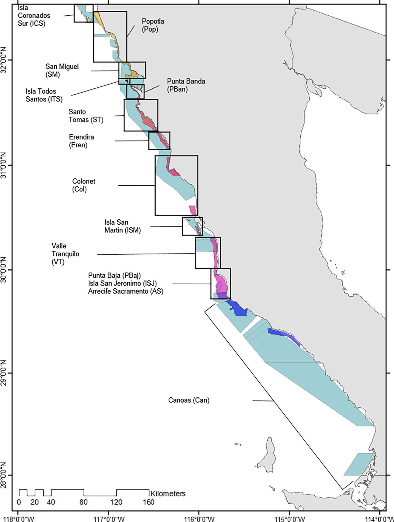
Figure 1 Red sea urchin and spiny lobster authorized fishing areas.
Kelp biomass data (Macrocystis pyrifera) were estimated monthly using Landsat satellite imagery to estimate canopy biomass across the study area at 30 m resolution, from 2000 to 2018 following methods described by Cavanaugh et al. (2011) and Bell et al. (2020). Kelp forest were delimited into two zones depending on biomass levels: Outer kelp forest and core kelp forest.
Daily catch records for California sheephead (Semicossyphus pulcher), kelp bass (Paralabrax clathratus), and spiny lobster (Panulirus interruptus) were acquired through Mexico’s National Transparency Platform1. The database includes the date, catch in kg, landing site, and the number of vessels used for fishing. California sheephead and kelp bass are fished under ‘finfish’ commercial permits, mainly with hook and line onboard artisanal vessels, with a small midrange finfish fleet of 25 boats. Spiny lobster fishing can be done under commercial fishing permits or concessions only with authorized traps within the authorized fishing area. The three species are caught in all Baja California, including Guadalupe and Cedros Islands; but these two sites were excluded from the analysis since there is no red urchin catch reported for those sites.
Sheephead and kelp bass catch data were geolocalized, assuming a higher abundance of sheephead in the outer zones of the kelp forests, while kelp bass inhabits the middle and outer zones of the forest (Claisse et al., 2012). Based on catch records landing sites and species, the catch was assigned a random location either outer or in the core zones of the kelp forests surrounding landing sites. Spiny lobster catches were geo-located based on each permit holder’s fishing area; given that traps are not placed inside kelp forests nor dropped too deep Cavanaugh et al. (2011; 2013), kelp-covered areas and depths greater than 300 m were not included. Due to authorized landing sites or fishing areas, it was necessary to group sheephead and spiny lobster data sites in the following groups: 1) Isla Coronados Sur and Popotla (ICS-Pop), 2) San Miguel-Isla Todos Santos–Punta Banda–Santo Tomas–Erendira-Colonet (SM-Col), 3) Punta Baja-Isla San Jeronimo–Arrecife Sacramento (PBaj-As). All catch and landing data presented come from commercial fishing records, since there is no registry of sustenance fishing for red sea urchins or lobsters, and these species are prohibited in recreational fisheries. Sheephead and kelp bass are also fished in recreational fisheries (see Rosales–Casián and Gonzalez–Camacho, 2003), but no records exist. Therefore, we considered all catch and landing data as total catches.
California sheephead and kelp bass catch information were curated to remove misplaced dates stored as catch or as the number of vessels or highly unlikely catch values (e.g., one vessel with an average max. capacity of 1.2 ton reporting 5 ton in one single day trip). This was done by cross-referencing with permit holder databases2 and catch records. It is important to note that due to the way landings are reported, it is very difficult to discern whether an artisanal vessel lands many times or if many artisanal vessels are landing one time each. Reports on coastal fishing in Baja California are nonexistent, and very few reports on artisanal fishing have been conducted, focused only on schooling fish or expensive invertebrates (Rosales–Casián and Gonzalez–Camacho, 2003). The case for spiny lobster fisheries data was no different; extensive cross-referencing and data curation were also needed.
Site-specific sea surface temperature (SST) data was gathered monthly from multisensory SST time series for 2000 to 2018 (4 km pixel, daylight at 11µ; from sensors AVHRR, MODIS Terra, MODIS Aqua and VIIRS Suomi-NPP). Images were processed in SEDAS (7) following Karu et al. (2015) and Karu et al. (2012) criteria. Wave power (CgE) represents the wave energy flux on the entire water column, better reflecting the action of waves over the selected sites; we hypothesize that the most substantial expected effects of waves are on kelp itself, not directly on the invertebrates on the bottom. For that reason, wave power selected over other metrics. Data was obtained from the IOWAGA hindcast (Rascle & Ardhuin, 2013), produced by the French Research Institute for the Exploitation of the Sea, Ifremer. The hindcast is based on global multigrid implantation of the Wave Watch 3 model, with ~18 km spatial resolution in the study area. Wave power is computed every 3hrs from wave directional spectra S(f,θ):
where ρ is water density (≈1024), g is gravity acceleration (≈9.8 m s-1), and Cg is the group velocity. For each site, the closest model node was chosen to represent wave power at that site. All sites were closer than 8 km from the chosen node.
Upwelling index (upw) data was gathered from NOAA’s Environmental Research Division (https://oceanview.pfeg.noaa.gov/products/upwelling/intro, “Accessed 20 Jan 2019”). We used the traditional Bakun (1973, 1975) upwelling index time series for two nodes: 33 and 30° N, as they were the closest stations to the Baja California kelp forest locations. This index is calculated with Eakman’s theory of mass transport due to wind stress; positive values can be considered as the amount of water that is upwelled, while negative values imply downwelling.
Multivariate El Niño Index (MEI) data was gathered from NOAA’s Earth System Research Laboratory (http://www.esrl.noaa.gov/psd/enso/mei/, “Accessed 20 Jan 2019”). MEI was selected due to the importance of El Niño/Southern Oscillation (ENSO) as a phenomenon causing global climate variability on inter-annual timescales (Wolter and Timlin, 1993, Wolter and Timlin, 1998). MEI is based on the six main observed variables over the tropical Pacific: sea level pressure, zonal and meridional components of surface wind, sea surface temperature, surface air temperature, and total cloudiness fraction of the sky (Wolter and Timlin, 1993, Wolter and Timlin, 1998).
North Pacific Gyre Oscillation (NPGO) data were obtained from KNMI Climate Explorer3 for the same period as the other variables.
All data for each site were summarized monthly and yearly and we calculated standardized anomalies for biological, local, and regional variables, based on the American Meteorological Society definition of anomaly as the deviation of (usually) temperature or precipitation in a given region over a specified period from a long-term average from the same region (AMS, 2022), using the formula:
where the total time series average µ is subtracted from each value xi and divided by the standard deviation of the time series. Indexes such as MEI and NPGO are already presented as standardized anomalies. All further analyzes were conducted using standardized anomalies.
We built correlation matrices and correlation network plots between all variables using the packages Corrr (Kuhn et al., 2020) and Ggraph (Lin Pedersen, 2020) in R Core Team (2022) (Ver. 4.2.1, 2022).
We implemented generalized linear models (GLM), with full-time series of all variables, as:
where rsu is the density of the red sea urchin population for month i, year j, site k; ϵi is the random error under the effect of Urchin.ct, Calsh.ct, Kelpsbs.ct, Lobst.ct, SST, CgE, Upw, MEI, and NPGO for month i, year j, site k, respectively; β0…10 are parameters to be estimated. All variables were entered as standardized anomalies.
We developed specific models based on SST variability that depict different climatological conditions: 1) Preheat wave (normal conditions), 2) Heatwave (as defined by Hobday et al., 2016), and 3) Post–heat wave. During each condition, we identified sites that presented average SST, as well as sites that were above (+1 SD) and below average SST (-1 SD), during the different thermal events (Figure 2, S2). We implemented a GLM with the same structure used for the full-time series with data corresponding to each climatological condition.
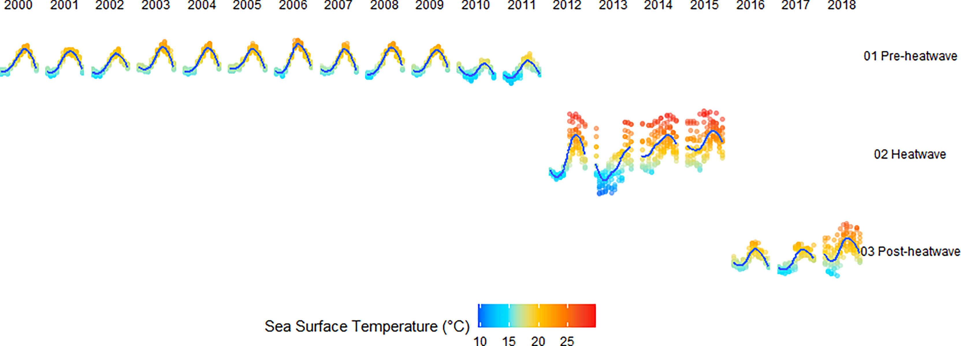
Figure 2 Monthly time series of sea surface temperature for all sites. The thermal periods and conditions analyzed are indicated. Red tones represent above-average SST sites; blue tones represent below-average SST sites. The average SST is shown as a blue line.
An Analysis of the Residual Sum of Squares (ARSS) was used to compare between models. This analysis tests whether two or more curves are statistically different (Zar, 1984).
Time lags between possible effects of the selected variables on red sea urchin population density were explored using the cross-correlation functions in R (2020); trends and seasonality were removed from all variables to avoid overlapping effects.
We examined the causality of the variables that were determined to affect the density of the population of red sea urchins through the GLMs, using the CausalImpact package (Brodersen, et al., 2015; Brodersen and Hauser, 2020) in R. This is a Bayesian structural time series model approach that allows inferring the causal impact an ‘intervention’ has exerted on an outcome metric over time, based on a diffusion-regression state-space model that predicts the counterfactual response in a synthetic control that would have occurred without an intervention (Brodersen et al., 2015). It models the behavior that the response variable might have in the absence of the possible effects produced by the predictor variables. As stated by Brodersen et al. (2015), the structural time-series models allow examination of the time-time series and flexibly choosing appropriate components for trend, seasonality, and the type of regression (static or dynamic) for the controls. Posterior inference in the model is performed by simulating draws of the model parameters and the state vector given by the observed data; afterward, posterior simulations are used to simulate the posterior predictive distribution over the counterfactual time series given the pre-intervention activity. The posterior predictive samples are used to compute the posterior distribution of the pointwise impact for each time step; the same samples are used to obtain the posterior distribution of cumulative impact (Brodersen et al., 2015). We considered red sea urchin population density (rsu) as the response variable, and the significant variables from GLMs to be the predictor variables to assess their impact on rsu as an outcome metric over four “interventions”: the full-time series, pre-heatwave, heatwave, and post-heatwave periods.
Results
The monthly average kelp biomass for the 2000–2018 period was 391 tons; yearly kelp biomass averaged 4,695 tons throughout the period. We observed high values of kelp biomass (> 7,500 tons) in ISM and PBan; intermediate values (3,000-5,000 tons) were common in ICS, Pop, VT, PBaj-ISJ, AS, and Can; the lowest biomass was observed in Col. Kelp forest delimitation was based on biomass levels for 2000-2018; areas with average kelp biomass of 270 to 680 tons/ha were common in the outer kelp forest and ranged from 800 to 1,300 ton/Ha at the core (Figure 3A). Red sea urchin population density was high at PBan and ITS (averaging +4 urchins m-2), compared to the rest of the sites that showed densities below two urchins m-2. Sites like ISJ and Can showed very low densities (<1 urchin m-2) (Figure 3B). The red urchin catches were high (more than 200 tons) in ST, PBaj, and AS, and low (below 20 tons) at ICS and ISJ. Sheephead catches were high (above 50 tons) at PBaj-AS and SM-COL, and low (below 5 tons) at ICS-Pop. Seabass catches were high (60 tons) in Can, approximately 10 tons in Col and Pbaj, and less than 5 tons in the rest of the sites. Spiny lobster catches were high (75 tons) in PBaj – ISJ – AS, about 50 tons at SM-COL and Can, and below 25 tons at ISM; the rest of the sites showed very low catches (Figure 3).
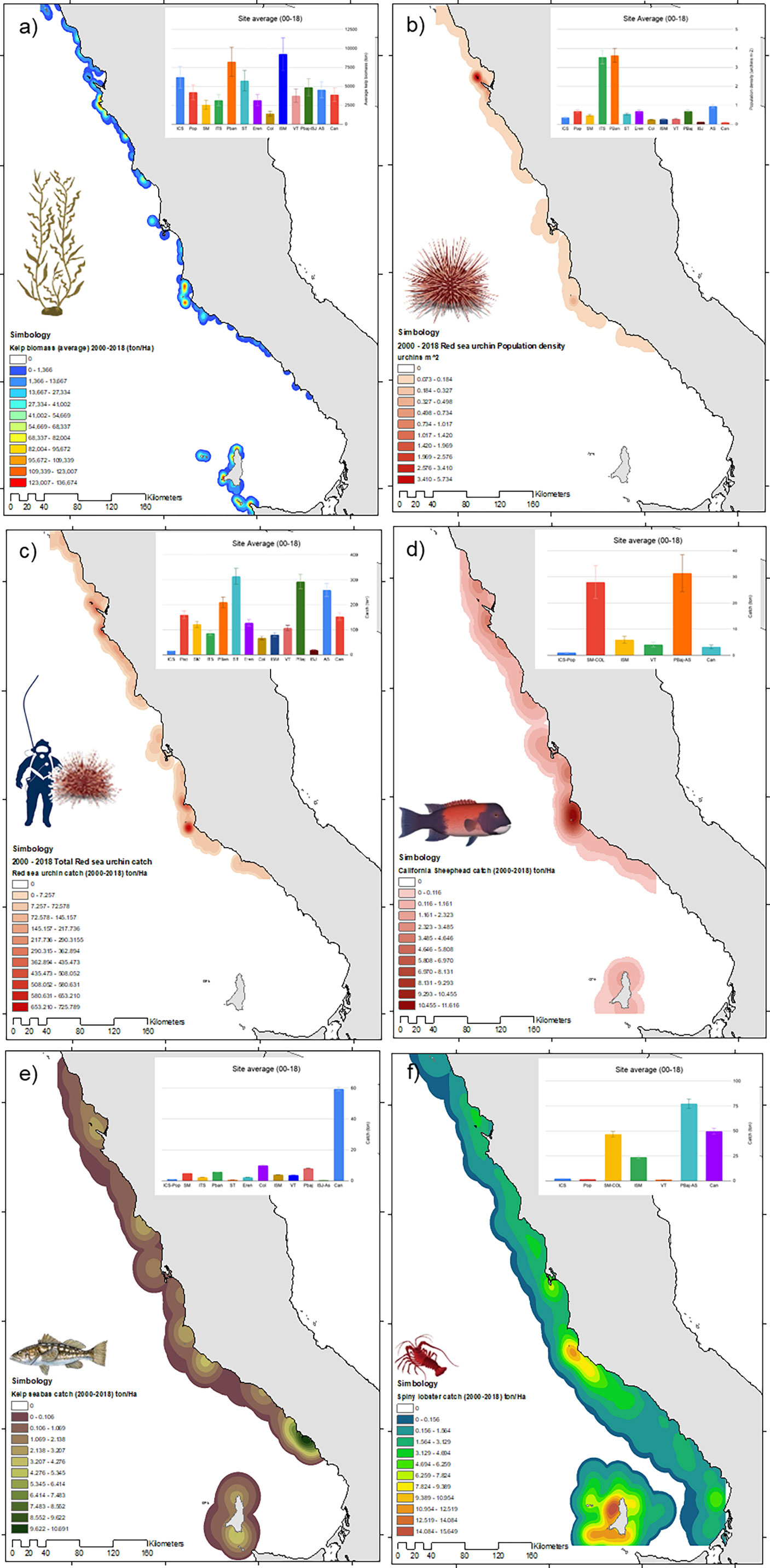
Figure 3 Distribution and density of (A) Kelp biomass, (B) population density of red sea urchin, (C) red urchin catch, (D) California sheephead, (E) kelp bass, and (F) spiny lobster catch, along the Pacific coast of Baja California. Data for 2000-2018.
The standardized anomalies for kelp biomass were positive for 8 years; although no identifiable pattern was evident, positive anomalies were observed for four consecutive years (2007-2010), with high values in 2005 and 2009. In 2016, there were high negative anomalies. The sites with positive kelp biomass anomalies were ICS, PBan, ST, and ISM (Figures 4A, G). Red sea urchin population density anomaly was negative from 2000 to 2008, and shifted to positive values from 2009 to 2015, after this year, anomalies returned to negative values. ITS, PBan, and AS displayed positive anomalies for the period (Figures 4B, H). No identifiable pattern was observed with sheephead and kelp bass catch anomalies, both showed positive anomalies for 7 years; however, anomalies occurred in different years, further, anomalies from 2016 to 2018 were inverse for both species. SM-Col and PBaj-AS showed positive sheephead catch anomalies, while mainly Can have positive kelp bass catch anomalies during the analyzed period (Figures 4C–E, I–K). We observed negative anomalies in spiny lobster from 2000 to 2010, the trend shifted to positive catch anomalies from 2011 to 2018. SM-Col, PBaj-As, and Can were the only sites with positive catch anomalies for the period (Figures 4F, L).
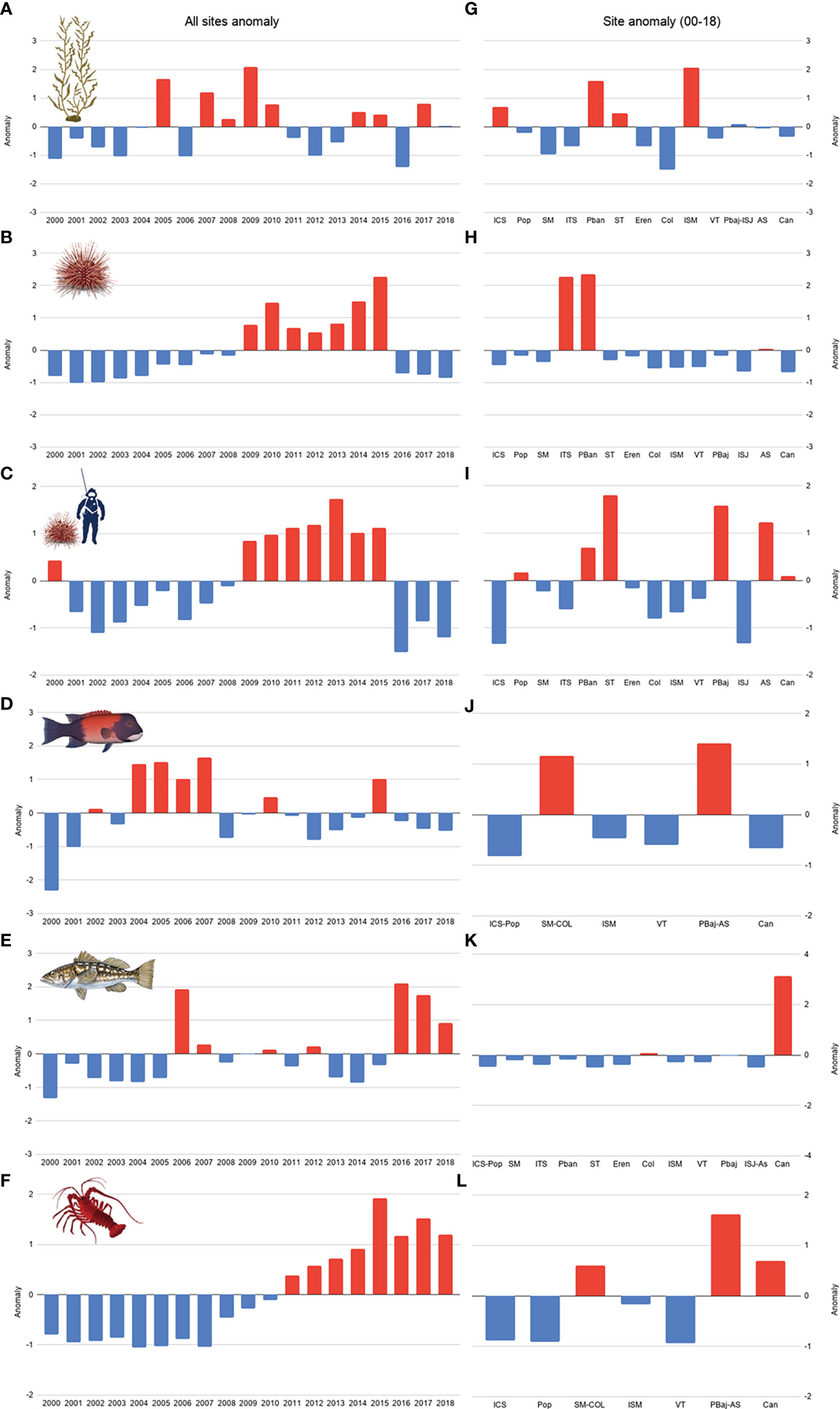
Figure 4 Kelp biomass (A), red sea urchin population density (B) and catch (C), California sheephead (D), kelp bass (E) and spiny lobster catch (F) anomalies from 2000 to 2018- and 19-year site anomaly (G-L, respectively).
We observed high variability in environmental variables during the study period. Yearly average SST ranged from 16.7 to 22.4°C, with higher values during 2014, 2015, and 2018 (21.4, 22.4, and 19.8°C, respectively), years with anomalies higher than two. The sites with positive SST anomalies for the whole period were ICS-Pop, SM, PBan, Eren, Col, and VT, the last three sites were the ones with higher anomalies. High negative anomalies were observed at ITS, PBaj, and ISJ-AS. The average CgE for the entire period ranged from 9.4 to 14.3 kw m-1, with positive anomalies from 2000 to 2006, except in 2004 with a slightly negative anomaly. From 2007–2018, the anomalies were negative; however, 2010 and 2016 showed the greatest positive anomalies of the period, greater than 2 units. Positive anomalies were observed at 4 sites: PBan, ISM, PBaj, and ISJ-AS, where the anomaly was almost 2 units. The average upwelling index ranged from 105.5 to 143.6 m-3 per 100 m coastline; positive anomalies were higher in 2007 and 2012, and high negative values were observed in 2004, 2014, and 2015. A regional pattern was evident, with northern sites more exposed to positive upwelling index anomalies and southern sites with negative values. The average annual MEI values showed two periods of positive anomalies in 2002–2004 and 2015-2016; while positive anomalies were more common from 2000–2004 and 2007–2013; during this period (2007-2013), the upwelling index and NPGO showed inverse anomaly patterns (Figure 5).
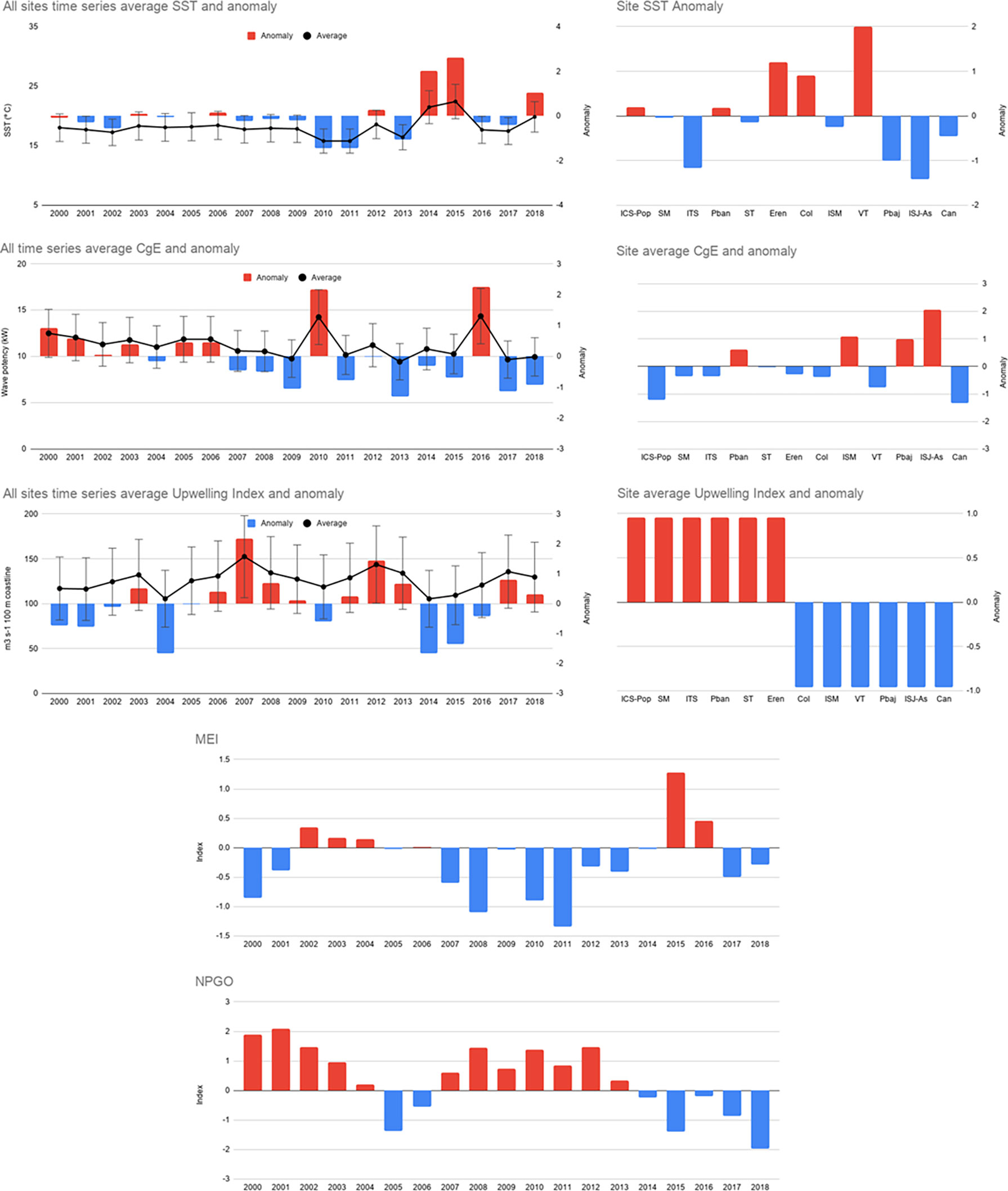
Figure 5 Local (Average SST, CgE), regional (Upwelling index), and oceanic (MEI, NPGO) variables values and anomalies from 2000 to 2018 and 19-year site anomaly.
Correlations and time lag of significant variables
Patterns were evident when comparing the density of red sea urchins with all variables analyzed (Table 1) and their time lags (S1). Urchin catch was the variable with a higher correlation (0.7-0.9) with red sea urchin density in all scenarios, with time lags between 0 and 8 months. Although the strength of the correlation with SST was variable, it was positive for all scenarios, and it was high (> 0.5) for the heatwave and above-average scenarios with a lag ranging from 5 months to 1.5 years. The correlation of kelp biomass with urchin density was always positive, although low (0-0.2), with time lags from 2 months to 1.5 years. Lobster catch correlation was always positive and ranged from 0.2 to 0.4, with time lags from 0 to 1 year. Seabass catch was always positively correlated, although low (0.1-0.3), and no correlation was observed for the full-time series and heatwave scenarios. The sheephead catch was positive and low (0.1-0.3) for most scenarios with lags of 3 to 4 months, except under the average conditions when it was negative (-0.2). The correlation with NPGO was negative in the full-time series (-0.1), heat wave (-0.5), and below-average scenarios (-0.2) and positive under average conditions (0.1); no correlation was found for the rest of the scenarios. The correlation with MEI was positive and low (0.1-0.3) in most of the scenarios, and high (0.6) under heatwave conditions, with time lags between 0 to 4 months. The correlation with the upwelling index and CgE was negative and low (0.1-0.4) for all scenarios (Tables 1, S1). Other correlations among variables that were significant were sheephead–kelp bass catch (0.3), sheephead–spiny lobster catch (-0.4), and kelp bass–spiny lobster catch (-0.3), SST and spiny lobster (0.4), kelp biomass and the upwelling index (0.4), urchin catch and upwelling index (-0.4), SST and MEI (0.4); MEI and NPGO were negatively correlated (-0.3). These correlations changed depending on the time frame or location of each model (Figure 6).
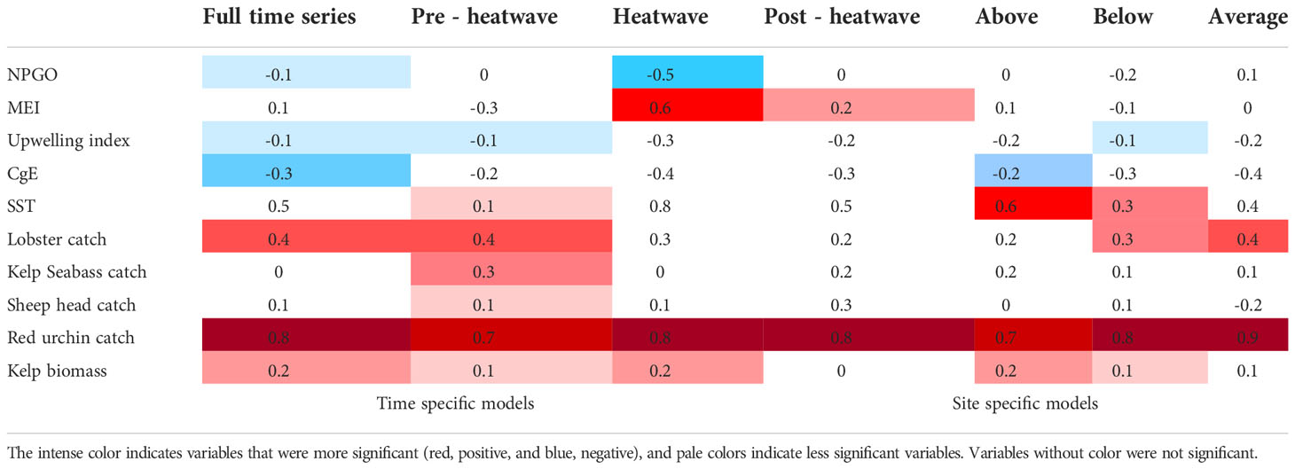
Table 1 Summary of correlations between red sea urchin density and estimated variables under time-specific and location-dependent thermal conditions.
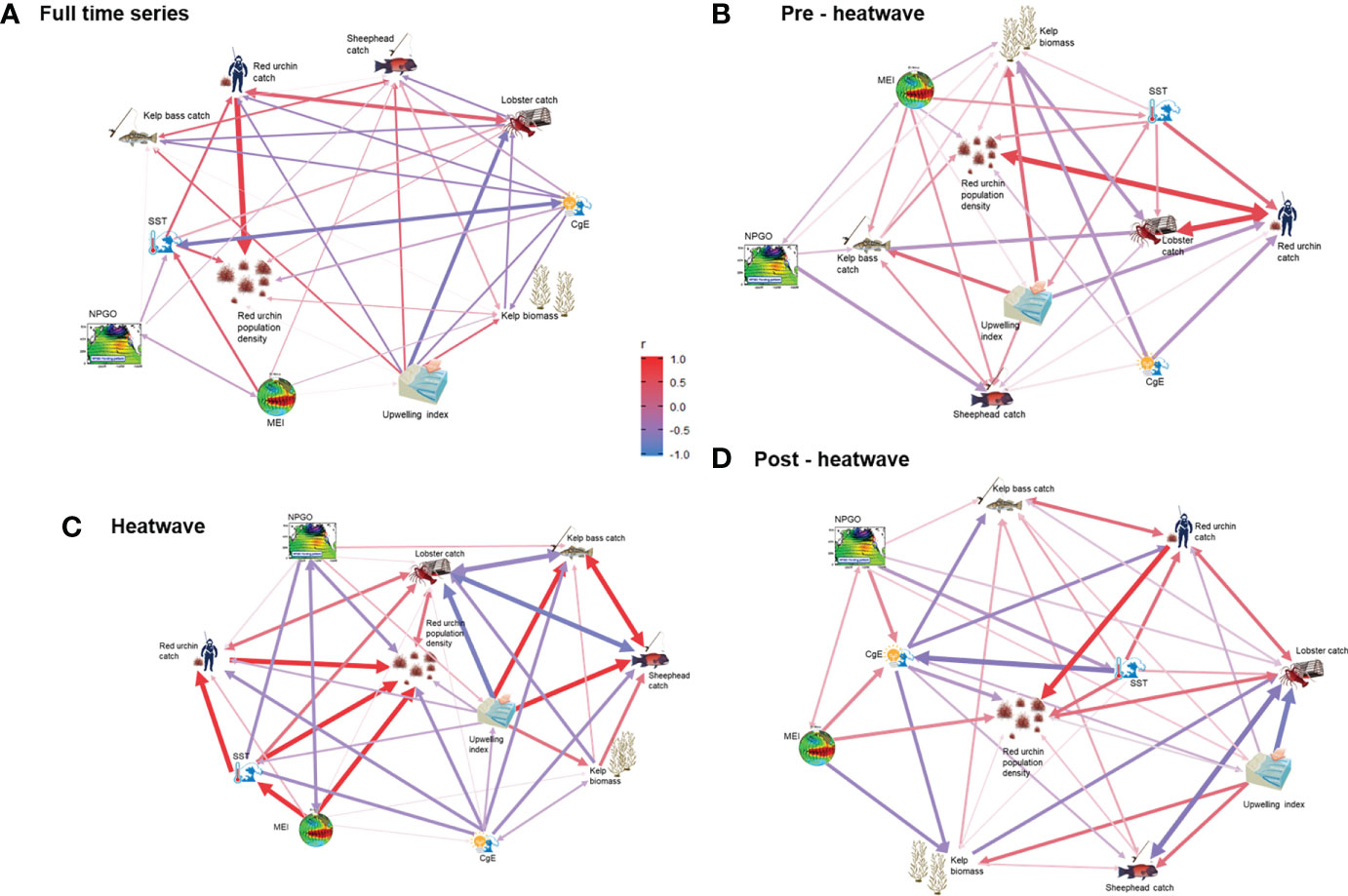
Figure 6 Correlogram of variables that could influence the abundance of red sea urchins along the Pacific coast of Baja California. Correlations were analyzed under different conditions: (A) Full-time series (2000–2018); (B) Pre–heatwave (2000–2011); (C) Heatwave (2012–2015); (D) Post–heatwave (2016–2018).
Time specific analysis
Generalized linear models (GLMs) and relative importance
Significant variables changed depending on the models; the model that showed the highest number of significant variables was GLM00-11 (before the heat wave), while GLM16-18 (after the heat wave) showed the lowest number of significant variables (Table 2).
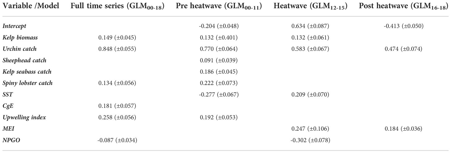
Table 2 Significant variables in time-specific GLM, coefficients (± errors). Only significant variables’ coefficients and intercepts are shown.
Causal impact
Variables that were significant for the entire time series account for 65.75% of the observed variability. The red sea urchin catch accounted for most of the variability observed in the density of the red sea urchin population, with spiny lobster, kelp biomass, and upwelling index accounting for less than 20% of the model’s R2. Significant variables in the pre-heatwave model account for 73.25% of the observed variability. Red sea urchin catch continued to be one of the most important variables in the model, followed by lobster catch, SST, kelp bass, and sheephead. During the heatwave, significant variables accounted for 90.03% of the observed variability; red urchin catch continued to be the most important variable, followed by SST, NPGO, and MEI. Significant variables during the post-heat wave period account for 82.17% of the observed variability, with red sea urchin catch being the most important variable, followed by MEI (Figure 7).
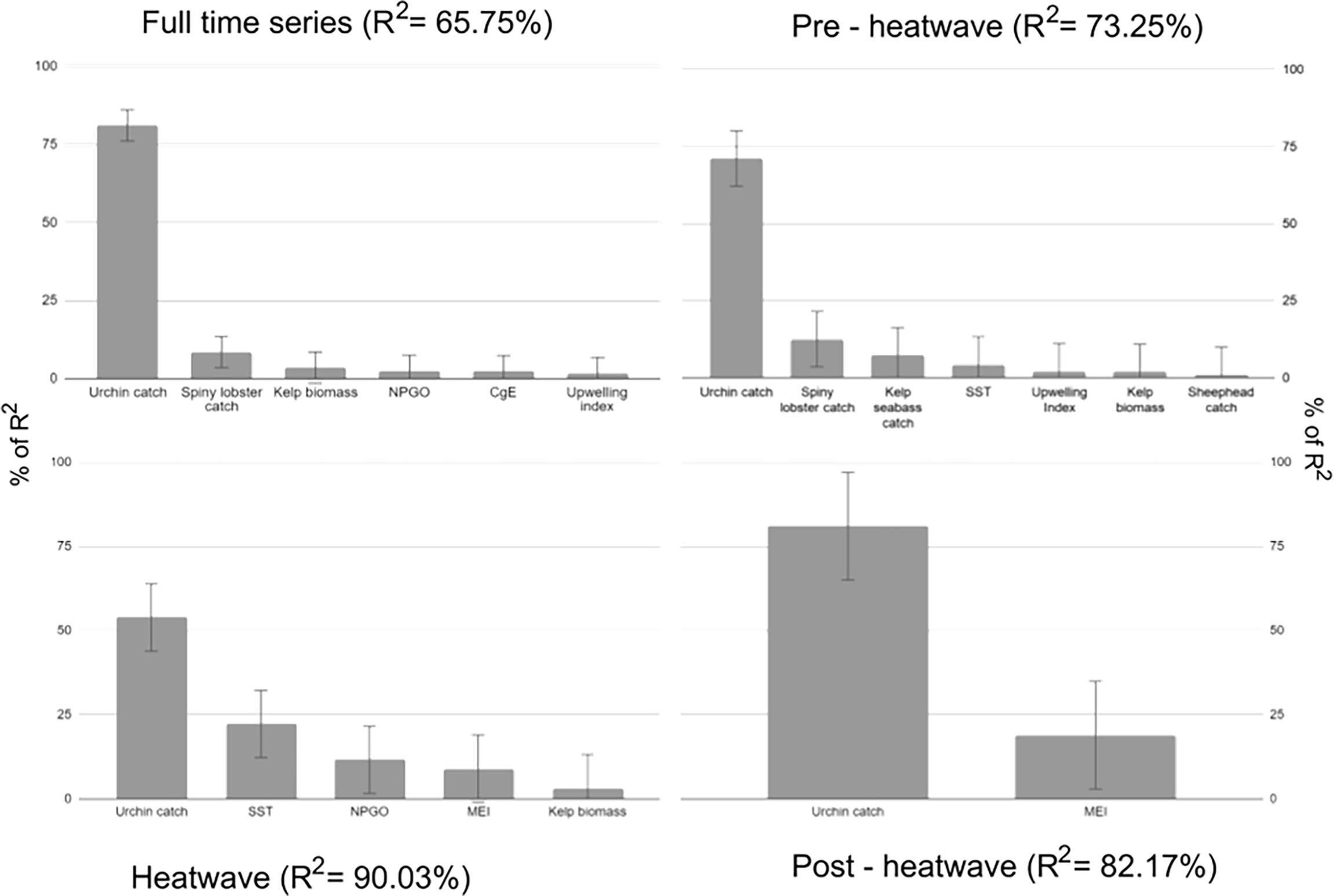
Figure 7 Share of R2 (as a percentage) of significant variables for all models. Metrics are normalized to sum 100% for each scenario. Whiskers represent 95% CI limits.
Causal impact analysis in full-time series GLM00-18 revealed that significant variables as a whole had a positive impact on red sea urchin density anomaly (rsu), with an average value of 0.011; in the absence of the effects of these variables, the expected value was -0.64. The average causal effect of these variables on rsu was 0.65 (-0.24≤µ≤1.47). Analysis on Pre–heatwave conditions GLM00-11 revealed that significant variables as a whole had a positive impact on red sea urchin density anomaly, with an average value of -0.16; in the absence of the effects of these variables, the expected value was -0.84. The average causal effect of these variables on rsu was 0.68 (-0.54≤µ≤1.36). During the heatwave GLM12-15, the analysis revealed that the significant variables had a positive impact on rsu, with an average value of 1.13; In the absence of this effect, rsu was 0.60. The average causal effect of significant variables on rsu was 0.53 (0.25≤µ≤0.83). Analysis of postheatwave conditions GLM16-18 revealed that, as a whole, significant variables had a negative impact on rsu, with an average value of -0.62; in the expected absence of this effect, the average value of rsu was 1.04. The average causal effect of these variables on rsu was -1.66 (-2.20≤µ≤-1.19). The probability of obtaining these effects by chance is very small, which suggests the effects can be considered significant (Figure 8).
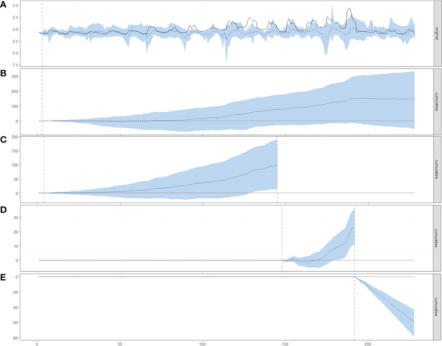
Figure 8 (A) Original time series with a counterfactual estimate (dotted line and shaded area) and cumulative results of the causal impact on red sea urchin population density anomaly (dotted) and confidence intervals at 95% (shaded) for (B) full-time series, (C) Pre – heatwave, (D) Heatwave, and (E) Post – heatwave models and significant variables; horizontal axis are the number of months from Jan-2000 (0) to December-2018 (229). The dotted vertical line indicates where the causal effect was tested.
Comparison between models
Having determined the relative importance of the variables on each time frame, we modeled rsu using specific important variables for the full-time series and heatwave conditions. Comparison between predicted values of the full models (GLM00-18) and condition-specific (GLM00-11 | GLM12-15 | GLM16-18) suggested that these approaches were significantly different (ARSS, F2,0.05 = 34.04, p<0.001), with the condition-specific models showing better fit (R2 = 0.78; Figure 9).
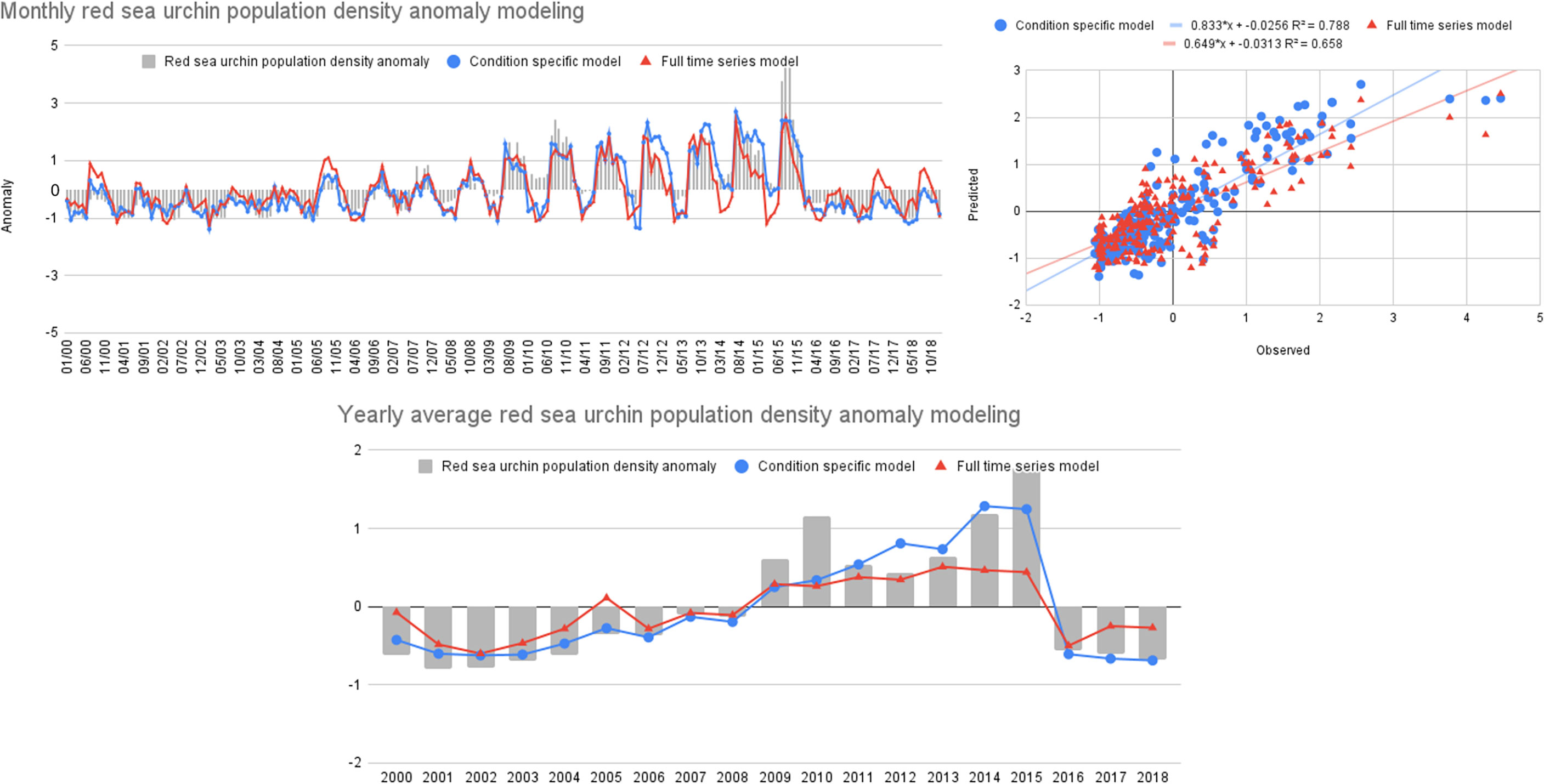
Figure 9 Comparison between observed density of red sea urchin population anomaly (bars), and predicted values from full-time series (▲) and Condition-specific (•) models.
Discussion and conclusions
Our results show that red sea urchin population density in Baja California is subject to different environmental, biological, and anthropogenic sources of variability, in the form of changing thermal conditions, wave energy exposure, upwelling, food availability (kelp biomass), different levels of predator abundance and fishing pressure. Despite the overall urchin population density trend, site-specific biological and environmental information displayed high variability within and among sites. This has also been observed in other kelp ecosystems where environmental variation at fine (depth within sites), local (within locations), and regional scales (among locations) will influence where urchins can affect macroalgae assemblages, regardless of predator density and fishing intensity (Shears et al., 2008). Time and space scenarios reveal that the importance of significant variables shifts depending on thermal environmental conditions. During the pre-heatwave period, biological variables such as red urchin predators and food (kelp biomass) were important to explain red urchin variability; in contrast, during the heatwave period, environmental variables were more relevant (SST, NPGO, and MEI). During the post-heatwave period, the importance of both biological and environmental variables diminishes, and none were significant. These results suggest that under extreme conditions, the red urchin population is mainly driven by local temperature and oceanic scale variables. The importance of variables is also site-specific; however, the local temperature was important at all sites.
The fishery
Our results indicate that, in all scenarios analyzed, urchin catch is the most crucial factor affecting red sea urchins, compared to other tested variables. In northern Washington, harvest has been observed to reduce sea urchin densities, where sites under experimental harvest showed a reduction between 93.7 and 96.3% (Carter and VanBlaricom, 2002). Harvest also affects size distribution significantly by reducing between 15 and 73% the density of legal-size urchins in northern and southern California (Tegner and Dayton, 1981; Pfiester and Bradbury, 1996). Furthermore, red sea urchin density, adult size, and gonadosomatic index (GSI) within MPAs are greater compared to unprotected sites (Teck et al., 2017). Our results agree with this evidence suggesting that fishing pressure is a key driver in controlling red sea urchins throughout the fishing geographic range.
Harvest depends not only on urchin density but also on roe yield and quality, fishable days due to weather, and market conditions (Kato, 1972; Kato and Schroeter, 1985; Kalvass and Hendrix, 1997; Kalvass and Rogers-Bennett, 2001; Andrew et al., 2002; Schroeter et al., 2009; Medellín–Ortiz et al., 2020). Roe yield depends entirely on food availability (kelp and drift kelp; see Rennick et al., 2022), and is determined by the diver in a pre-harvest sampling at the beginning of the dive. If 3 of 5 randomly selected urchins in the patch have orange-yellow gonads that fill over 80% of the urchin, then the patch is harvested; otherwise, the diver moves to another area. This behavior can result in low catches and high areas of ‘skinny’ urchin density. Inter-annual differences in urchin density have been reported in different areas in the study region for 2003, 2005, 2006, and 2008, and have been related to fishing intensity and recruitment rates in each site (Palleiro-Nayar et al., 2012). There is no assessment of recruitment rates, frequency, or patterns for red sea urchins in Baja California, however, the observed catch trends for the period being analyzed here could be related to constant settlement and recruitment (Medellín–Ortiz et al., 2020), and consistent with Southern California’s recruitment patterns observed by Ebert et al. (1994). Also, Medellín–Ortiz et al. (2020), found that over-harvesting in some sites depleted temporarily legal-size urchins without altering population recruitment. This effect has also been described for red sea urchins in Southern California (DeWees, 2004; Stevenson et al., 2016).
The intricate relationship between urchin divers and the density of the urchin population needs a different interpretation considering the absence of sea otters in the region (Gallo-Reynoso, 1997) and low levels of abundance of other important predators such as California sheephead and spiny lobster (Alonzo et al., 2004; present study).
Temporal effects
We observed a lagged effect on the density of the red sea urchin population from important variables in models specific to time and thermal conditions. These lagged effects ranged from two months to two years depending on the scale of the variable; being local variables made the effects noticeable after months (e.g. SST), while regional and oceanic variables took longer to produce an effect on the densities of red sea urchins (e.g. upwelling index, MEI). In Baja California, many factors can intervene for El Niño to have an effect, and depend mainly on the geographic extent of the Kelvin wave that may or may not travel northward from the Equator (Wang, 2003). This region also experienced the recent warming event known as ‘the Blob’ (Marine heatwave, MHW), which traveled from north to south along the California Current System (Bond et al., 2015; Oliver et al., 2018). These two events and the delay in which they arrive in Baja California might have differential effects on northern and southerly distributed urchins. In the presence of events of such magnitude, our results suggest that local variables become more important than oceanic variables, especially in locations where even during these extreme events, the SST remained below average values. SST was important during extreme conditions (heatwave) and sites with above-average SST. The temperature has been shown to have direct effects on red sea urchin metabolic rates, with an increase in oxygen consumption as temperature increases, suggesting a temperature-dependent metabolism (Ulbricht and Pritchard, 1972). It has also been suggested that red sea urchins may display different temperature preferences between day and night, moving away from unfavorable physiological temperatures (Salas et al., 2012). These thermal effects have also been observed in red sea urchin embryos, where high temperatures increased the body size of prism-stage embryos, suggesting that moderate warming may improve the growth and thermal tolerance of red sea urchins (Wong and Hofmann, 2020). Although it has been stated that increased temperatures resulting from El Niño or MHW have negative impacts on red sea urchins (Tegner and Dayton, 1987; Okamoto et al., 2020), our results suggest that red sea urchins might benefit from increased temperatures, with increased metabolic rates and increased size “heat adapted” larvae that would result in the increasing urchin densities observed in our study. However, temperatures above 28°C for a prolonged time have adverse effects on red sea urchins, causing reduced movement from tube feet and increased movement through spines and death (Hernández et al., 2004).
Kelp
Kelp biomass was highly variable among sites and through time. Although it suffered negative impacts from heatwaves, its resilience was spatially variable and was not significantly related to SST metrics, indicating that local-scale environmental and biotic processes could play a larger role in kelp recovery as described by Cavanaugh et al. (2019), who found that spatial patterns of resistance in giant kelp were better explained by an absolute thermal threshold (mean SST of the warmest month) than by relative increases in temperature as measured by SST anomalies and heatwave days. They suggest that local adaptation to heat stress did not have a major impact on the response of kelp to this warming event throughout much of its range. Our results show that the variability of kelp biomass was not highly correlated with red sea urchin density, and it was observed as a significant variable during the heat wave period and in the above-average temperature scenario. This might be related to red sea urchins’ ability to feed as an active grazer or consume hidden drifting algae, so satellite-based kelp biomass estimations and variability do not necessarily reflect changes in food availability from drift kelp fronds that are a significant urchin food source, and an indicator of the level of nourishment of the urchins (Harrold and Reed, 1985). These authors describe that sea urchins in kelp-dominated areas are well nourished, move little, occupy cracks and crevices, and probably feed on drift algae, compared to those urchins found in barrens, where drift algae are sparse, and poorly nourished sea urchins actively graze the exposed substratum (Watanabe and Harrold, 1991), and subsist on coralline algae in the absence of kelp (Harrold and Reed, 1985). Furthermore, high-density urchin aggregations are a prerequisite to destructive grazing (Dean et al., 1984), and cause cavitation damage on the holdfast of kelp, increasing kelp mortality due to storms or even intense wave action, causing kelp to dislodge and produce urchin ‘barrens’ (Tegner et al., 1995). Drift kelp (detrital supply) has been identified as a key factor in the foraging behavior of sea urchins that changes from passive feeding when detritus is abundant, to causing a significant reduction in kelp biomass by active grazing on living kelp when detritus is scarce (Rennick et al., 2022). The grazing activity of red sea urchins in Baja California has not been evaluated, and since the reproductive potential of individual sea urchins is closely tied to food availability (Rogers-Bennett et al., 1995), it becomes necessary to assess the grazing behavior of red sea urchins as well as the amount, seasonality, and importance of drift kelp in the diet of red sea urchins in Baja California.
Predators
Urchin predator’s harvest was important under the pre-heatwave conditions only. According to Rosales–Casián and Gonzalez–Camacho (2003), California sheephead and kelp bass accounted for 25.9 and 10.6% of the finfish caught in Baja California, respectively, and ranked 3.5 based on their Index of Community Importance (ICI) values. They also describe San Quintín, San Martin Island, and Punta Baja as important finfish fishing sites. Our results show that Punta Baja (PBaj) and Canoas (Can) are important fishing sites for California sheephead and kelp bass, respectively; however, low catch levels at other sites could be attributable to high levels of fishing (Alonzo et al., 2004) and the decline of cold-water species due to climatic events such as El Niño and the Blob (Arafeh–Dalmau et al., 2019). Sheephead fishing has affected size-structured interactions with sea urchins in Southern California, reducing sizes and altering sheephead life histories that lead to increased urchin densities (Hamilton and Caselle, 2015). Spiny lobster harvest has been proposed to trigger a trophic cascade leading to increased urchin densities and decreased macroalgal biomass (Tegner and Levin, 1983; Tegner and Dayton, 2000; Behrens and Lafferty, 2004; Guenther et al., 2012). This response has been observed in Bahia Asuncion (Baja California Sur), where higher densities of spiny lobster led to increased abundances of kelp (Jenkinson et al., 2020). The effect that fishing simultaneously on multiple urchin predators has on the red urchin population has not been evaluated. In this work, we integrated catches of urchin predators to evaluate their importance in explaining urchin density variability and found that these variables were correlated with urchin density only during the pre-heatwave scenario, suggesting that under ‘average temperature’ conditions the effect of fishing on predators and, consequently, on urchin density is higher than local temperature, the most important variable during warm conditions.
Model choices
Although aggregated models are widely applied to understand, predict and manage populations and marine ecosystems, they fall short if the underlying system exhibits non-linear dynamics (Ye and Sugihara, 2016). Furthermore, the model output can underestimate variability and overestimate stability (Griffith, 2020). Our condition-specific model was better at reproducing estimated red sea urchin density; this might be related to its ability to capture condition-specific variability (normal conditions vs. heatwave, post-heatwave conditions) by using only the variables that were significant and relatively important in such conditions, instead of averaging out variability and considering that the effects of all variables remain the same through time (assumption made in the full-time series model). Although some variables had low correlations, the effect of different combinations of variables on the densities of red sea urchins was considered statistically significant by causal impact analysis. While this type of analysis has been mainly used in the market analysis (eg. Märkle-Huß et al, 2018; Schmitt et al, 2018; Martín Cervantes and Cruz Rambaud, 2020), the characteristics of marketing data match those of biological survey data: often observational, rarely following the ideal of randomized design, subject to multiple seasonal variations, and are often affected by unobserved variables and their interactions. While correlations have been one of the most commonly used statistical techniques in biological studies (see Yadav, 2018), the similarity between biological and marketing data makes the causal impact analysis suitable for biological data, and its use in our field should be further explored.
Conclusion
The relative importance and significance of variables were different depending on the time frame or site analyzed. These differences in importance were related to the variability in time and space of each variable. Understanding how ecological and fisheries systems behave and interact becomes even more critical in the face of environmental changing conditions. Separating the environmental effects of fishing on natural populations is key to increasing the protection of natural ecosystems and improving fisheries management.
This study suggests that in Baja California, red sea urchin harvest has become the most important control of the red sea urchin population, so efforts should be encouraged and supported by state and federal agencies must encourage and support efforts to promote more resilient ecosystems in the face of environmental uncertainty. It is paramount that the people responsible for filling out landing logs understand the importance of accurate and timely reporting. Improving fisheries-dependent data collection and quality may reduce uncertainty in estimates of population status, fishing effort, and fishing mortality of harvested species. Such improvements can be achieved through participation in capacity-building workshops to increase permit-holder engagement and compliance with already established landing logs. It is also important to promote fisheries-independent surveys that might yield information on urchin density, kelp, sheephead, kelp bass, and lobster abundance to fine-tune stock assessment models, as well as efforts to forecast population abundance and ecosystem trends under different scenarios of environmental variability and climate change. Such surveys would benefit from the participation of community-based monitors from each fishing cooperative, fishing group, or permit holder, with the support of other stakeholders. Improving management of the commercial species that inhabit kelp forest, could yield benefits for the entire ecosystem, fishers, and the red sea urchin population in Mexico.
Data availability statement
The original contributions presented in the study are included in the article/Supplementary Material. Further inquiries can be directed to the corresponding authors.
Author contributions
AM-O: Conceptualization, data acquisition, processing and analysis. Processing results, graphical interpretation, modeling, manuscript preparation, edition, revisions and submission. GM-M: Result interpretation, manuscript preparation, revisions. CA-F: Modeling advice, result interpretation, manuscript preparation and revisions. ES-d-A: SST data acquisition, processing and curation. Results interpretation, manuscript preparation and revisions. HG-N: wave potency data acquisition, processing and curation. Results interpretation, manuscript preparation and revisions. RB-L: Manuscript revisions, editing. K-C: kelp biomass data acquisition, processing and curation. Manuscript revisions, editing. All authors contributed to the article and approved the submitted version.
Funding
This research project was conducted under CONACyT scholarship No. 442284, while in UABC's Coastal Oceanography Graduate Program, and UABC's internal Fund. Project #647. Open access publication fees were provided by Pronatura Noroeste A.C. serving the objectives of the Baja California sea urchin Fisheries Improvement Project sponsored by the Marine Stewardship Council's Ocean Stewardship Fund.
Acknowledgments
We would like to thank all the divers, finfish, and lobster fishermen in Baja California; We also like to acknowledge Pronatura Noroeste A.C. for its participation in fulfilling the objectives of the Baja California Sea Urchin Fisheries Improvement Project and its commitment to actively collaborate toward sustainable management of the red sea urchin fishery.
Conflict of interest
The authors declare that the research was conducted in the absence of any commercial or financial relationships that could be construed as a potential conflict of interest.
Publisher’s note
All claims expressed in this article are solely those of the authors and do not necessarily represent those of their affiliated organizations, or those of the publisher, the editors and the reviewers. Any product that may be evaluated in this article, or claim that may be made by its manufacturer, is not guaranteed or endorsed by the publisher.
Supplementary material
The Supplementary Material for this article can be found online at: https://www.frontiersin.org/articles/10.3389/fmars.2022.987242/full#supplementary-material
Footnotes
- ^ www.infomex.org.mx.
- ^ Publicly available at https://datos.gob.mx/busca/dataset/permisos-y-concesiones-de-pesca-comercial-para-embarcaciones-mayores-y-menores, and requested through Mexico’s National Transparency Institute: https://www.infomex.org.mx/gobiernofederal/home.action#
- ^ http://climexp.knmi.nl/getindices.cgi?WMO=O3Ddata/npgo&STATION=NPGO&TYPE=i&id=someone@somewhere; “Accessed 20 Jan 2019”.
References
Alonzo S. H., Key M., Ish T., MacCall A. D. (2004). Status of the California sheephead (Semicossyphus pulcher) stock (California Department of Fish and Game Report). Available at: www.dfg.ca.gov/mrd/sheephead2004.
American Meterological Society (AMS) (2022). Anomaly (Glossary of Meteorology). Available at: https://glossary.ametsoc.org/wiki/Anomaly.
Andrew N. L., Agatsuma Y., Ballesteros E., Bazhin A. G., Creaser E. P., Barnes D. K. A., et al. (2002). Status and management of world sea urchin fisheries. Oceanogr Mar. Biol. Annu. Rev. 40, 343–425.
Arafeh–Dalmau N., Montaño–Moctezuma G., Martínez J. A., Beas–Luna R., Schoeman D. S., Torres–Moye G. (2019). Extreme marine heatwaves alter kelp forest community near its equatorward distribution limit. Front. Mar. Sci. 6. doi: 10.3389/fmars.2019.00499
Bakun A. (1973). Coastal upwelling indices, west coast of north America (NOAA Technical Report), NMFS SSRF–671. US Department of Commerce.
Beas – Luna R., Micheli F., Woodson C. B., Carr M., Malone D., Torre J., et al. (2020). Geographic variation in responses of kelp forest communities of the California current to recent climatic changes. Glob. Change Biol. 00, 1–17. doi: 10.111/gcb.15273
Behrens M. B., Lafferty K. D. (2004). Effects of marine reserves and urchin disease on southern California rocky reef communities. Mar. Ecol. Prog. Ser. 279, 129–139. doi: 10.3354/meps279129
Bell T. W., Allen J. G., Cavanaugh K. C., Siegel D. A. (2020). Three decades of variability in california’s giant kelp forests from the landsat satellites. Remote Sens Environ. 238. doi: 10.1016/j.rse.2018.06.039
Bond N. A., Cronin M. F., Freeland H., Mantua N. (2015). Causes and impacts of the 2014 warm anomaly in the NE pacific, geophys. Res. Lett. 42, 3414–3420. doi: 10.1002/2015GL063306
Botsford L. W. (2001). Physical influences on recruitment to California current invertebrate populations on multiple scales. ICES J. Mar. Sci. 58, 1081–1091. doi: 10.1006/jmsc.2001.1085
Brodersen K. H., Gallusser F., Koehler J., Remy N., Scott S. L. (2015). Inferring causal impact using Bayesian structural time-series model. Ann. Appl. Stat vol. 9, 247–274. doi: 10.1214/14-AOAS788
Brodersen K. H., Hauser A. (2020). CausalImpact: Inferring causal effects using Bayesian structural time-series models package. version 1.2.4.
Carter S. K., VanBlaricom G. R. (2002). Effects of experimental harvest on red sea urchins (Strongylocentrotus franciscanus) in northern Washington. Fish Bull. 100, 662–673.
Castorani M. C. N., Reed D. C., Miller R. J. (2018). Loss of foundation species: disturbance frequency outweighs severity in structuring kelp forest communities. Ecology 99, 2442–2454. doi: 10.1002/ecy.2485
Cavanaugh K. C., Kendall B. E., Siegel D. A., Reed D. C., Alberto F., Assis. J. (2013). Synchrony in dynamics of giant kelp forests is driven by both local recruitment and regional environmental controls. Ecology 94 (2), 499–509. doi: 10.1890/12-0268.1
Cavanaugh K. C., Reed D. C., Bell T. W., Castorani and M. C. N., Beas-Luna R. (2019). Spatial variability in the resistance and resilience of giant kelp in southern and Baja California to a multiyear heatwave Front. Mar. Sci. 6, 413. doi: 10.3389/fmars.2019.00413
Cavanaugh K. C., Siegel D. A., Kinlan B. P., Reed D. C. (2010). Scaling giant kelp field measurements to regional scales using satellite observations. Mar. Ecol. Prog. Ser. Vol 403, 13–27. doi: 10.3354/meps08467
Cavanaugh K. C., Siegel D. A., Reed D. C., Dennison P. E. (2011). Environmental controls of giant-kelp biomass in the Santa Barbara Channel, California. Mar Ecol Prog Ser 429, 1–17. doi: 10.3354/meps09141
Chenillat F., Rivière P., Capet X., Di Lorenzo E., Blanke B. (2012). North pacific gyre oscillation modulates seasonal timing and ecosystem functioning in the California current upwelling system. Geophy. Res. Lett. Vol. 39, L01606. doi: 10.1029/2011GL049966
Claisse J. T., Pondella D. J. II, Williams J. P., Sadd J. (2012). Using GIS mapping of the extent of nearshore rocky reefs to estimate the abundance and reproductive output of important fishery species. PLoS One 7 (1), e30290. doi: 10.1371/journal.pone.0030290
Cowen R. K. (1983). The effect of sheephead (Semicossyphus pulcher) predation on red sea urchin (Strongylocentrotus franciscanus) populations: an experimental analysis. Oecologia 58, 249–255. doi: 10.1007/BF00399225
Cowen R. K. (1985). Large Scale pattern of recruitment by the labrid semicossyphus pulcher: causes and implications. J. Mar. Res. 43, 719–742. doi: 10.1357/002224085788440376
Davenport A. C., Anderson T. W. (2007). Positive indirect effects of reef fishes on kelp performance: The importance of mesograzers. Ecology Vol 88 (6), 1548–1561. doi: 10.1890/06-0880
Dayton P. K. (1985a). The Structure and Regulation of Some South American Kelp Communities. Ecolo. Monogr. 55 (4), 447–468. http://www.jstor.org/stable/2937131
Dean T. A., Schroeter S. C., Dixon J. D. (1984). Effects of grazing by two species of sea urchins (Strongylocentrotus franciscanus and lytechinus anamesus) on recruitment and survival of two species of kelp (Macrocystis pyrifera and pterygophora californica). Mar. Biol. 78, 301–313. doi: 10.1007/BF00393016
DeWees C. M. (2004). Sea urchin fisheries: a California perspective. In: Lawrence J. M., Guzman O. (Eds.). Sea Urchins: fisheries and ecology. DEStech Publications, Lancaster. Pp 37–55
Di Lorenzo E., Schneider N., Cobb K. M., Franks P. J.S., Chhak K., McWilliams J. C., et al. (2008). North Pacyfic Gyre Oscillation links ocean climate and ecosystem change. Geophysical Research Letters. 35(8), L08607. doi: 10.1029/2007GL032838
Ebeling A. W., Laur D. R., Rowley R. J. (1985). Severe storm disturbances and reversal of community structure in a southern California Kelp forest. Mar. Biol. 84, 287–94. doi: 10.1007/BF00392498
Ebert T. A., Schroeter S. C., Dixon J. D., Kalvass P. (1994). Settle-ment patterns of red and purple sea urchins (Strongylo-centrotus franciscanus and S. purpuratus) in California, USA. Mar. Ecol. Prog. Ser. 111, 41–52. https://www.int-res.com/articles/meps/111/m111p041.pdf
Eisaguirre J. H., Eisaguirre J. M., Davis K., Carlson P. M., Gaines S. D., Caselle J. E. (2020). Trophic redundancy and predator size class structure drive differences in kelp forest ecosystem dynamics. Ecology 101 (5), e02993. doi: 10.1002/ecy.2993
Estes J. A., Duggins D. O. (1995). Sea Otters and kelp forests in Alaska: Generality and variation in a community ecological paradigm. Ecol. Monogr. 65 (1), 75–100. doi: 10.2307/2937159
Estes J. A., Palmisano J. F. (1974). Sea Otters: their role in structuring near shore communities. Science 185, 1058–1060. doi: 10.1126/science.185.4156.1058
Free C. M., Thorson J. T., Pinsky M. L., Oken K. L., Wiedenmann J., Jensen O. P. (2019). Impacts of historical warming on marine fisheries production. Science 363, 979–983. doi: 10.1126/science.aau1758.
Gallo – Reynoso J. P. (1997). Situation and distribution of otters in Mexico, with emphasis on lontra longicaudis annectens, MAJOR 1897. Rev. Mexicana Mastozoologia 2, 10–32. doi: 10.1111/j.1748-7692.1997.tb00639.x
Griffith G. P. (2020). Closing the gap between causality, prediction, emergence, and applied marine management. ICES J. Mar. Sci. 77(4), 1456–1462. doi: 10.1093/icesjms/fsaa087
Grove R. S., Zabloudil K., Norall T., Deysher L. (2002). Effects of El niño events on natural kelp beds and artificial reefs in southern California. ICES J. Mar. Sci. 59, S333–S337. doi: 10.1006/jmsc.2002.1290
Guenther C. M., Lenihan H. S., Grant L. E., Lopez – Carr D., Reed D. C. (2012). Trophic cascades induced by lobster fishing are not ubiquitous in southern California kelp forests. PLoS One 7 (11), e49396. doi: 10.1371/journal.pone.0049396
Hamilton S. L., Caselle J. E. (2015). Exploitation and recovery of sea urchin predator has implications for the resilience of southern California kelp forests. Proc. R. Soc B. 282, 20141817. doi: 10.1098/rspb.2014.1817
Harrold C., Reed D. C. (1985). Food availability, sea urchin (Strongylocentrotus franciscanus) grazing and kelp forest community structure. Ecology 66, 1160–1169. doi: 10.2307/1939168
Hereu B., Linares C., Sala E., Garrabou J., Garcia – Rubies A., Diaz D., et al. (2012). Multiple processes regulate long – term population dynamics of sea urchins on Mediterranean rocky reefs. PLOS ONE 7, 5. doi: 10.1371/journal.pone.0036901
Hernández M., Bückle F., Guisado C., Barón B., Estavillo N. (2004). Critical thermal maximum and osmotic pressure of the red sea uchin strongylocentrotus franciscanus acclimated at different temperatures. J. Thermal Biol. 29, 231–236. doi: 10.1016/j.thebio.2004.03.003
Hilborn R., Amoroso R. O., Anserson C. M., Baum J. K., Branch T. A., Costello C., et al. (2020). Effective fisheries management instrumental in improving fish stock status. PNAS Vol 117 (4), 2218–2224. doi: 10.1073/pnas.1909726116
Hilborn R., Walters C. J. (1992). Quantitative Fisheries Stock Assessment. Springer New York. 570 pp. doi: 10.1007/978-1-4615-3598-0
Hobday A. J., Alexander L. V., Perkins S. E., Smale D. A., Stratub S. C., Oliver E. C. J., et al. (2016). A hierarchical approach to defining marine heatwaves. Prog. Oceanography Vol. 141, 227–238. doi: 10.1016/j.pocean.2015.12.014
Hobsom E. S., McFarland W. N., Chess J. R. (1981). Crepuscular and nocturnal activities of California near shore fishes, with consideration of their scotopic visual pigment and the photic environment. US Fish Bull. 79, 1–30.
Jenkinson R. S., Hovel K. A., Dunn R. P., Edwards M. S. (2020). Biogeographical variation in the distribution, abundance, and interactions among key species on rocky reefs of the northeast pacific. Mar. Ecol. Prog. Ser. Vol. 648, 51–65. doi: 10.3354/meps13437
Jiménez – Quiroz M. C., Palleiro – Nayar J. S., Salgado – Rogel M. L., Rodríguez – Buendía A. (2013). Natural mortality of red sea urchin from Baja California, méxico, estimated with in situ and satellite measured temperature. Hidrobiológica 23 (3), 443–445.
Kalvass P. E., Hendrix J. M. (1997). The California red sea urchin, strongylocentrotus franciscanus, fishery: catch, effort and management trends. Mar. Fish Rev. 59 (2), 1–17.
Kalvass P. E., Rogers-Bennett L. (2001). “Red sea urchin. pp. 101-104 and 560-561,” in California's living marine resources: A status report. Eds. Leet W. S., DeWees C. M., Klingbeil R., Larson E. J. (Sacramento: California Dept. of Fish and Game. ANR Publ), SG01–SG11.
Kahru M., Kudela R. M., Anderson C. R., Mitchell B. G. (2015). Optimized merger of ocean chlorophyll algorithms of MODIS-Aqua and VIIRS. IEEE Geoscience and Remote Sensing Letters 12, 11. doi: 10.1109/LGRS.2015.2470250
Kahru M., Di Lorenzo E., Manzano-Sarabia M., Mitchell B. G. (2012). Spatial and temporal statistics of sea surface temperature and chlorophyll fronts in the California Current. J. of Plankton Research 34 (9), 749–760. doi: 10.1093/plankt/fbs010
Kato S., Schroeter S. C. (1985). Biology of the red Sea urchin, strongylocentrotus franciscanus, and its fishery in California. Mar. Fisheries Rev. 47 (3), 1–20.
Ladah L. (2003). The shoaling of nutrient-enriched subsurface water as a mechanism to sustain primary productivity off central Baja California during El nin ã o winters. J. Mar. Syst. 42, 145–152. doi: 10.1016/S0924-7963(03)00072-1
Ladah L., Zertuche-Gonzalez J., Hernández-Carmona G. (1999). Giant kelp (Macrocystis pyrifera, phaeophyceae) recruitment near its southern limit in Baja California after mass disappearance during ENSO 1997–1998. J. Phycol 35, 1106–1112. doi: 10.1046/j.1529-8817.1999.3561106.x
Lafferty K. D. (2004). Fishing for lobsters indirectly increases epidemics in sea urchins. Ecol. Appl. 14 (5), 1566–1573. doi: 10.1890/03-5088
Lin Pedersen T. (2020). Ggraph: An implementation of grammar of graphics for graphs and networks package. version 2.0.3.
Lowe C. G., Topping D. T., Cartamil D. P., Papastamatiou Y. P. (2003). Movement patterns, home range, and habitat utilization of adult kelp bass paralabrax clathratus in a temperate no-take marine reserve. Mar. Ecol. Prog. Ser. 256, 205–216. doi: 10.3354/meps256205
Märkle-Huß J., Feurriegel S., Neumann D. (2018). Contract durations in the electricity market: Causal impact of 15min trading on the EPEX SPOT market. Energy Economycs Vol 69, 367–378. doi: 10.1016/j.eneco.2017.11.019
Martín Cervantes P. A., Cruz Rambaud S. (2020). An empirical approach to the “Trump effect” on US financial markets with causal-impact Bayesian analysis. Heliyon Vol. 6 (8), e04760. doi: 10.1016/j.heliyon.2020.e04760
Medellín-Ortiz A., Montaño-Moctezuma G., Alvarez-Flores C., Santamaria-del-Angel E. (2020). Retelling the history of the red Sea urchin fishery in Mexico. Front. Mar. Sci. 7. doi: 10.3389/fmars.2020.00167
Mendoza–Carranza M., Rosales–Casian J. A. (2002). Feeding ecology of juvenile kelp bass (Paralabrax clathratus) and barred sand bass (P. nebulifer) in punta banda estuary, Baja California, Mexico. Bull. South. California Acad. Sci. Vol. 101, 103–117.
Nichols K. D., Segui L., Hovel K. A. (2015). Effects of predators on sea urchin density and habitat use in a southern California kelp forest. Mar. Biol. 162, 1227–1237. doi: 10.1007/s00227-015-2664-2
Okamoto D. K., Reed D. C., Schroeter S. (2020). Geographically opposing responses of sea urchin recruitment to changes in ocean climate. Limnol Oceanogr 9999, 1–6. doi: 10.1002/lno.11440
Oliver E. C., Donat M. G., Borrows M. T., Moore P. J., Smale D. A., Alexander L. V. (2018). Longer and more frequent marine heatwaves over the past century. Nat. Commun. 9, 1324. doi: 10.1038/s41467-018-03732-9
O’Malley J. M. (2009). Spatial and temporal variability in growth of Hawaiian spiny lobsters in the northwestern Hawaiian islands. Mar. Coast. Fisheries 1:1, 325–342. doi: 10.1577/C09-031.1
Palleiro-Nayar J. S., Montaño-Moctezuma G., Sosa-Nishizaki O. (2012). Variación espacio temporal de la densidad de erizo rojo Strongylocentrotus franciscanus (Echinodermata: Echinoidea: Strongylocentrotidae) en Baja California. Hidrobiologica 22(1), 28–34. http://www.redalyc.org/articulo.oa?id=57824412004
Pérez-Matus A., Carrasco S. A., Gelcich S., Fernandez M., Wieters E. A. (2017). Exploring the effects of fishing pressure and upwelling intensity over subtidal kelp forest communities in central Chile. Ecosphere 8 (5), e01808. doi: 10.1002/ecs2.1808
Pérez-Matus A., Pledger S., Díaz F. J., Ferry L. A., Vásquez J. A. (2012). Plasticity in feeding selectivity and trophic structure of kelp forest associated fishes from northern Chile. Revista Chilena de Historia Natural 85, 29–48. doi: 10.4067/S0716-078X2012000100003
Pfister C. A., Altabet M. A., Weigel B. L. (2019). Kelp beds and their local effects on seawater chemistry, productivity, and microbial communities Vol. 0 (Ecology). doi: 10.1002/ecy.2798
Pfister C. A., Bradbury A. (1996). Harvesting red sea urchins: recent effects and future predictions. Ecol. Appl. 6 (1), 298–310. doi: 10.2307/2269573
R Core Team (2020). R: A language and environment for statistical computing. R Foundation for Statistical Computing, Vienna, Austria. Available at: http://www.R-project.org/.
Rascle N., Ardhuin F. (2013). A global wave parameter database for geophysical applications. Part 2: Model validation with improved source term parameterization. Ocean Model. 70, 174–188. doi: 10.1016/j.ocemod.2012.12.001
Rennick M., DiFiore B. P., Curtis J., Reed D. C., Stier A. C. (2022). Detrital supply suppresses deforestation to maintain healthy kelp forest ecosystems. Ecology Vol 103 (5), e3673. doi: 10.1002/ecy.3673
Rogers – Bennett L., Bennett W. A., Fastenau H. C., Dewes C. M. (1995). Spatial variation in red sea urchin reproduction and morphology: implications for harvest refugia. Ecol. Appl. 5, 1171–1180. doi: 10.2307/2269364
Rosales – Casián J., Gonzalez – Camacho J. R. (2003). Abundance and importance of fish species from artisanal fishery on the pacific coast of northern Baja California. Bull. South. California Acad. Sci. 102 (2), 51–65.
Salas A., Diaz F., Re A. D., Gonzalez M., Galindo C. (2012). Thermoregulatory behavior of red Sea urchin strongylocentrotus franciscanus (Agassiz 1863) and purple Sea urchin strongylocentrotus purpuratus (Stimpson 1857) (Echinodermata: Echinoidea). Open Zoology J. 5, 42–46. doi: 10.2174/1874336601205010042
Schiel D. R., Andrew N. L., Foster M. S. (1995). The structure of subtidal algal and invertebrate assemblages at the Chatham Islands, New Zealand. Marine Biology 123, 355–367. doi: 10.1007/BF00353627
Schmitt E., Tull C., Atwater P. (2018). Extending Bayesian structural time-series estimates of causal impact to many-household conservation initiatives. Ann. Appl. Stat Vol. 12 (4), 2517–2539. doi: 10.1214/18-AOAS1166
Schroeter S. C., Gutiérrez N. L., Robinson M., Hilborn R., Halmay P. (2009). Moving from data poor to data rich: A case study of community-based data collection for the San Diego red Sea urchin fishery. Mar. Costal Fisheries: Dynamics Management Ecosystem Sci. 1, 230–234. doi: 10.1577/C08-037.1
Shears N. T., Babcock R. C., Salomon A. K. (2008). Context-dependent effects of fishing: Variation in trophic cascades across environmental gradients. Ecol. Appl. 18 (8), 1860–1873. doi: 10.1890/07-1776.1
Steneck. R. S., Graham M. H., Bourque B. J., Corbett D., Erlandson J. M., Estes J. A., et al. (2002). Kelp forest ecosystems: biodiversity, stability, resilience and future. Environ. Conserv. 29 (4), 436–459. doi: 10.1017/S0376892902000322
Stevenson C. F., Demes K. W., Salomon A. K. (2016). Accounting for size-specific predation improves our ability to predict the strength of a trophic cascade. Ecol. Evol. 6 (4), 1041–1053. doi: 10.1002/ece3.1870
Teck S. J., Lorda J., Shears N. T., Bell T. W., Cornejo-Donoso J., Caselle J. E., et al. (2017). Disentangling the effects of fishing and environmental forcing on demographic variation in an exploited species. Biol. Conserv. 209, 488–498. doi: 10.1016/j.biocon.2017.03.014
Tegner M. J., Dayton P. K. (1987). El Niño effects on southern California kelp forest communities. Adv. Ecol. Res. 17, 243–279. doi: 10.1016/S0065-2504(08)60247-0
Tegner M. J., Dayton P. K. (1991). Sea Urchins, El niños, and the long term stability of southern California kelp forest communities. Mar. Ecol. Prog. Ser. Vol 77, 49–83. doi: 10.3354/meps077049
Tegner M. J., Dayton P. K. (1981). Population structure, recruitment and mortality of two sea urchins (strongylocentrotus franciscanus and s. purpuratus) in a kelp forest. Mar. Ecol. Prog. Ser. 5 (3), 255–268. https://www.jstor.org/stable/24813148
Tegner M. J., Dayton P. K., Edwards P. B., Riser K. L. (1995). Sea urchin cavitation of giant kelp (Macrocystis pyrifera C. Agardh) holdfasts and its effects on kelp mortality across a large California forest. Journal of Experimental Marine Biology and Ecology. 191(1), 83–99. doi: 10.1016/0022-0981(95)00053-T
Tegner M. J., Dayton P. K. (2000). Ecosystem effects of fishing in kelp forest communities. ICES J. Mar. Sci. 57, 579–589. doi: 10.1006/jmsc.2000.0715
Tegner M. J., Dayton P. K., Edwards P. B., Riser K. L. (1997). Large-Scale, low-frequency oceanographic effects on kelp forest succession: a tale of two cohorts. Mar. Ecol. Prog. Ser. 146, 117–134. doi: 10.3354/meps146117
Tegner M. J., Levin L. A. (1983). Spiny lobsters and sea urchins: analysis of a predator–prey interaction. J. Exp. Mar. Biol. Ecol. 73, 125–150. doi: 10.1016/0022-0981(83)90079-5
Ulbricht R., Pritchard A. W. (1972). Effect of temperature on the metabolic rate of sea urchins. Biol. Bull. 142, 178–185. doi: 10.2307/1540254
Wang B. (2003). “Kelvin waves,” in Encyclopedia of meteorology. Ed. Holton. J. (New York, NY: Academic Press), 1062–1067.
Watanabe J. M., Harrold C. (1991). Destructive grazing by sea urchins strongylocentrotus spp. in a central California kelp forest: potential roles of recruitment, depth and predation. Mar. Ecol. Prog. Ser. 71, 125–141. doi: 10.3354/meps071125
Wolter K., Timlin M. S. (1993) Monitoring ENSO in COADS with a seasonally adjusted principal component index. Proc. of the 17th Climate Diagnostics Workshop, Norman, OK, NOAA/NMC/CAC, NSSL, Oklahoma Clim. Survey, CIMMS and the School of Meteor., Univ. of Oklahoma, 52–57. https://psl.noaa.gov/enso/mei/WT1.pdf
Wolter K., Timlin M. S. (1998). Measuring the strength of ENSO events - how does 1997/98 rank? Weather. 53, 315–324. doi: 10.1002/j.1477-8696.1998.tb06408.x
Wong J. M., Hofmann G. E. (2020). The effects of temperature and pCO2 on size, thermal tolerance and metabolic rate of the red sea urchin (Mesocentrotus franciscanus) during early development. Mar. Biol. 167, 33. doi: 10.1007/s00227-019-3633-y
Yadav S. (2018). Correlation analysis in biological studies. J. Pract. Cardiovasc. Sci. 4, 116–21. doi: 10.4103/jpcs_31_18
Ye H., Sugihara G. (2016). Information leverage in interconnected ecosystems: overcoming the curse of dimensionality. Science 353, 922–925. doi: 10.1126/science.aag0863
Young P. H. (1963). The kelp bass (Paralabrax clathratus) and its Fishery 1947– 1958. Fish Bulletin 122, 1–67.
Keywords: red sea urchin, fisheries, environmental variability, kelp forests, marine heatwaves, Baja California
Citation: Medellín–Ortiz A, Montaño–Moctezuma G, Álvarez–Flores C, Santamaría-del-Ángel E, García–Nava H, Beas–Luna R and Cavanaugh K (2022) Understanding the impact of environmental variability and fisheries on the red sea urchin population in Baja California. Front. Mar. Sci. 9:987242. doi: 10.3389/fmars.2022.987242
Received: 06 July 2022; Accepted: 02 November 2022;
Published: 24 November 2022.
Edited by:
Tanmay Sarkar, West Bengal State Council of Technical Education, IndiaReviewed by:
Kyle S. Van Houtan, Duke University, United StatesYukio Matsumoto, Japan International Research Center for Agricultural Sciences, Japan
Heng Wang, Dalian Ocean University, China
Copyright © 2022 Medellín–Ortiz, Montaño–Moctezuma, Álvarez–Flores, Santamaría-del-Ángel, García–Nava, Beas–Luna and Cavanaugh. This is an open-access article distributed under the terms of the Creative Commons Attribution License (CC BY). The use, distribution or reproduction in other forums is permitted, provided the original author(s) and the copyright owner(s) are credited and that the original publication in this journal is cited, in accordance with accepted academic practice. No use, distribution or reproduction is permitted which does not comply with these terms.
*Correspondence: Alfonso Medellín–Ortiz, YWxmb25zby5tZWRlbGxpbkB1YWJjLmVkdS5teA==; Gabriela Montaño–Moctezuma, Z21vbnRhbm9AdWFiYy5lZHUubXg=