Sea ice recognition for CFOSAT SWIM at multiple small incidence angles in the Arctic

Sea ice recognition is one of the main tasks for sea ice monitoring in the Arctic and is also applied for the detection of other ocean phenomena. The Surface Wave Investigation and Monitoring (SWIM) instrument, as an innovative remote sensor that operates at multiple small incidence angles, is different from existing sensors with moderate and normal incidence modes for sea ice monitoring. Sea ice recognition at small incidence angles has rarely been studied. Moreover, SWIM uses a discrimination flag of sea ice and sea water to remove sea ice from sea wave products. Therefore, this research focuses on sea ice recognition in the Arctic based on SWIM data from October 2020 to April 2021. Eleven features are first extracted, and applied for the analysis of the waveform characteristics using the cumulative probability distribution (CPD) and mutual information measurement (MIM). Then, random forest (RF), k-nearest neighbor (KNN) and support vector machine (SVM) classifiers are built, and their abilities of sea ice recognition are assessed. The optimal classifier is the KNN method with Euclidean distance and k equal to 11. Feature combinations are also used to separate sea ice and sea water based on the KNN method to select the optimal combination. Thus, the optimal classifier-feature assembly at each small incidence angle is established, and the highest overall accuracy reaches 97.1%. Moreover, the application of the optimal classifier–feature assemblies is studied, and its performance is fairly good. These assemblies yield high accuracies in the short- and long-term periods of sea ice recognition, and the overall accuracies are greater than 93.1%. So, the proposed method satisfies the SWIM requirement of removing the sea ice effect. Moreover, sea ice extents and edges can be extracted from SWIM sea ice recognition results at a high level of precision greater than 94.8%. As a result, the optimal classifier–feature assemblies based on SWIM data express the effectiveness of the SWIM approach in sea ice recognition. Our work not only highlights the new sea ice monitoring technology of remote sensing at small incidence angles, but also studies the application of SWIM data in sea ice services.

1 Introduction

Sea ice plays an important role in global climate change, shipping, navigation and the extraction of natural resources (Komarov and Buehner, 2021), and influences the detection of other ocean phenomena; for example, sea wave retrieval requires the removal of sea ice ‘pollution’ (Ren et al., 2021; Wang J.K., et al., 2021). Thus, sea ice recognition has become a main task performed to meet the scientific and operational requirements of national and commercial ice services, which provides sea ice edge, extent, and concentration products (Cheng et al., 2020; de Gélis et al., 2021). Microwave remote sensors, including synthetic aperture radar (SAR), scatterometers, and altimeters, have become the main tools used for sea ice monitoring in the Arctic. These sensors operate at incidence angles of 0° or 20–60°. SAR is an imaging radar with multiple bands including L, C and X bands and a high spatial resolution of less than 1 m at 20–60°. Based on the available microwave backscattering information and image characteristics, SAR provides data mainly used to the regional distribution and change of the sea ice. Karvonen et al. (2005) proposed a segmentation technique based on intensity autocorrelation using C-band RADARSAT-1 SAR images; the accuracy of sea water recognition was 90%, and no results were reported for sea ice. Berg and Eriksson (2012) utilized a neural network to separate sea ice and sea water based on C-band ENVISAT and RADARSAT-2 SAR images, and the accuracies of sea ice and sea water identification were 87% and 94%, respectively. Asadi et al. (2021) proposed a multilayer perceptron (MLP) neural network for sea ice and sea water distinguishing based on RADARSAT-2 images, and the overall accuracy reached 82%. Komarov and Buehner (2021) presented a new method that could be applied at multiple spatial scales for automatic distinction between sea ice and sea water using RADARSAT-2 images, and the maximum overall accuracy reached 99%. At present, SAR has been used to obtain sea ice products for the Arctic region. Scatterometers can detect sea ice across the Arctic region at a coarse spatial resolution (several to tens of kilometers) and at two major frequencies: the C band (e.g., ASCAT and ERS-1/2) and the Ku-band (e.g., QuickSCAT and OSCAT). Sea ice recognition depends on the microwave backscattering powers of the horizontal and vertical polarizations, as well as the image reconstruction method (Gohin and Cavanie, 1994; Remund and Long, 1999; Rivas and Stoffelen, 2011; Otosaka et al., 2018). Haarpaintner and Spreen (2007) refined the detection method of low sea ice concentration using QuikSCAT data and improved the extraction accuracies of sea ice edges. Presently, operational sea ice edge, extent and concentration products in the Arctic have been generated for a long time, and sea ice recognition accuracies have reached 90% (Cavalieri et al., 1996; Breivik et al., 2012; Rivas et al., 2012; Remund and Long, 2014; Bi et al., 2018). Altimeters are mainly used for sea ice thickness retrieval based on large-scale and coarse spatial resolution observations similar to those of scatterometers; however, extracted sea ice and sea water information is needed to improve retrieval accuracies (Zhang et al., 2021). Some classifiers, such as the random forest (RF), k-nearest neighbor (KNN), and support vector machine (SVM) classifiers, are used for sea ice recognition based on the waveform features of echo signals which include the backscattering coefficient (σ₀), maximum power (MAX), pulse peakiness (PP), inverse mean power (IMP), leading edge width (LEW), and trailing edge slope (TES). The waveform features of airborne Ku-band radar altimeters were first used to discriminate the rough and smooth surfaces of sea ice, and a higher waveform peak and steeper trailing edge were associated with smooth surfaces (Drinkwater and Carsey, 1991). Laxon (1994) mapped sea ice extents based on PP and standard deviation of surface height extracted from ERS-1 radar altimeter data, which suggested clear operational applications in polar sea ice detection. Currently, the accuracies of sea ice and sea water recognition have reached 92% and 95%, respectively (Zygmuntowska et al., 2013; Rinne and Similä, 2016; Müller et al., 2017; Shen et al., 2017a; Shen et al., 2017b; Shu et al., 2019). However, the surface characteristics, snow coverage, and other factors certainly affect the stability of sea ice recognition accuracies, which needs further exploration. And these methods should be verified by more data in different study regions and long periods. Therefore, sea ice recognition using altimeters is still under study.

The Surface Wave Investigation and Monitoring (SWIM) instrument adopts a new observation mode with multiple small incidence angles (0° to 10°) for the detection of sea surface waves (Hauser et al., 2016; Hauser et al., 2017; Wang et al., 2019; Xu et al., 2019; Hauser et al., 2020). SWIM with a maximum latitude of 83°N can cover sea ice regions in the Arctic and be used for sea ice recognition. Moreover, SWIM sea wave products are influenced by the sea ice, resulting in that SWIM data should be labeled by the discrimination flag of sea ice and sea water. Thus, SWIM data with the new observation mode can be used for sea ice recognition and contribute to sea ice monitoring methods and operational techniques. Our previous study focused on sea ice type classification (Liu et al., 2021; Liu et al., 2022), and a method to distinguish between sea ice and sea water was not fully established. In addition, two new features (Inverse mean power, IMP; Trailing edge slope, TES) were introduced for first-year ice (FYI) and multiyear ice (MYI) separation, but these features were not used for sea water recognition. Therefore, based on our previous study, several key problems are explored in this study:

● New feature introduction and waveform analysis at small incidence angles to assess the use of different waveform features for separating sea ice and sea water;

● Classifier selection and assessment of the abilities for different classifiers with different settings;

● Establishment of the optimal classifier–feature assembly at each incidence angle; the assembly is established by combining the selected classifier and feature combinations. It can achieve sea ice recognition with high accuracy based on SWIM data obtained in the new detection mode;

● Application analysis of the optimal classifier–feature assemblies at small incidence angles, that is, whether these assemblies can be applied to remove sea ice from SWIM sea wave products and extract sea ice extents and edges for sea ice operational services.

Section 2 introduces the SWIM, SAR and sea ice chart data from the Arctic obtained between October 2020 and April 2021. Moreover, the waveform features of SWIM data are extracted, and classifiers for sea ice recognition are identified. Section 3 reveals the waveform analysis, and the overall accuracies of different classifiers and feature combinations, then, the optimal classifier-feature assembly for the SWIM data is established at each small incidence angle. Furthermore, the application of the optimal classifier-feature assemblies is also analyzed. Section 4 discusses the results in this study. Section 5 presents the conclusions and future work.

2 Data and methods

2.1 Data

There are three data sets used in this paper: SWIM, Sentinel-1 and sea ice chart data.

2.1.1 SWIM

The SWIM is loaded on the Chinese-French Oceanic Satellite (CFOSAT), which was successfully launched on October 29, 2018 (Wang et al., 2019; Xu et al., 2019). SWIM is the first spaceborne real aperture radar system that can operate at six small incidence angles (0° to 10°), the entire azimuth angle range (0–360°) and 13.575 GHz (Hauser et al., 2016; Hauser et al., 2017; Hauser et al., 2020). The main objective of SWIM is to provide wave spectra for the sea surface. SWIM spans nearly 90 km from 0° to 10° on the ground, and its footprint at 10° is approximately 18 km, as shown in Figure 1. SWIM can reach the northern and southern latitudes up to 83°. SWIM’s orbit assures a complete Earth coverage at the end of the cycle (13 days) except for small holes around the equator. The mid- and high-latitudes are very well covered as required by the mission. Level 1A SWIM data, which can be used to extract waveform features to recognize sea ice and sea water, are used in this study.

FIGURE 1

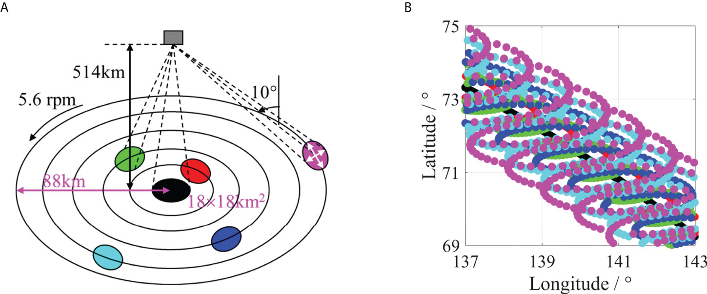
Figure 1 SWIM detection schematics for six incidence beams. (A) The projection geometries of the six beams in one macrocycle. One macrocycle represents six successive beams transmitting at small incidence angles with a discontinuous azimuth. (B) Samples of several macrocycles over the Earth’s surface (antenna aperture: 2°×2°).

2.1.2 Sentinel-1

Sentinel-1 was the first of five missions launched as part of the Copernicus Initiative of the European Commission (EC) and the European Space Agency (ESA). Sentinel-1 is in a near-polar, sun-synchronous orbit with a 12-day repeat cycle and 175 orbits per cycle for a single satellite. Sentinel-1A/B SAR can obtain all-weather, all-day images in the C-band in single-polarization (HH or VV) and dual-polarization (HH+HV or VV+VH) modes. Sentinel-1 SAR operates in four exclusive modes: stripmap (SM) mode, interferometric wide swath (IW) mode, extrawide swath (EW) mode and wave (WV) mode. Additionally, four products are provided: Level-0, Level-1 Single Look Complex (SLC), Level-1 Ground Range Detected (GRD) and Level-2 Ocean (OCN) data.

Sentinel-1A/B can support effective ice services, for example, the monitoring of sea ice extent, concentration and types in the Arctic (de Gélis et al., 2021, Li et al., 2021; Scharien and Nasonova, 2022). In this study, Sentinal-1 SAR images are used to evaluate sea ice recognition results of SWIM data. Considering the 18 km spatial resolution of SWIM products, we use the wide swath (about 400 km) and low resolution (about 90 m) SAR images of Lever-1 GRD products.

2.1.3 Sea ice charts

The sea ice charts used in this study are from the Arctic and Antarctic Research Institute (AARI) (AARI, 2022), and the National Snow and Ice Data Center (NSIDC) (Cavalieri et al., 1996; NSIDC, 2022).

(1) AARI

The AARI usually releases sea ice charts on Thursday. One sea ice chart covers three days from Sunday to Tuesday, including sea water and sea ice types (nilas, young ice, first-year ice and multiyear ice) in one Arctic ice year from October to April (AARI, 2022). In this study, only sea ice and sea water are separated in the Arctic from October 2020 to April 2021, and sea ice regions of different types are merged. During this period, thirty charts were issued, including 90 days. In general, multiyear ice (MYI) and sea water are the primary categories in the Arctic in October, and nilas (NI) and young ice (YI) only appear in small regions. Then, the sea ice rapidly develops from November to December. The sea ice distribution is stable from January to March and varies slowly in April. The characteristics of the sea ice distribution in April are similar to those from January to March. According to the characteristics of the sea ice distribution in the Arctic, sea ice development in one Arctic ice year can be divided into three stages: the first is October (Stage 1), the second is November to December (Stage 2), and the third is January to April (Stage 3).

(2) NSIDC

The NSIDC provides a sea ice concentration data set generated from the brightness temperature extracted from radiometer data, and one cell size is 25 ×25 km in the polar stereographic projection (Cavalieri et al., 1996; NSIDC, 2022). Notably, sea ice concentration products are generated daily. One cell where sea ice concentration is not lower than 15 percent is classified as sea ice, and the others are classified as sea water. Thus, the sea ice extents and edges are extracted and can be used to evaluate SWIM results.

2.1.4 Data matching and filtering

In this research, SWIM waveforms are matched and filtered for sea ice and sea water distinguishing in the Arctic based on the following criteria:

(1) SWIM data in the Arctic ice year from October 2020 to April 2021 are selected.

(2) The SWIM data in the coverage region of AARI sea ice charts are chosen. Then, these data are also matched to the observation time of each AARI sea ice chart in a three-day period from every Sunday to Tuesday mentioned in the Section 2.1.3.

(3) The waveforms of SWIM are labeled as sea ice or sea water based on matching with the AARI sea ice charts from the same dates. The sea ice distribution changes very slowly in the Arctic over three days in winter, especially when data with a coarse spatial resolution (tens of kilometers) are used. And, remote sensors with similar spatial resolution also do this method to obtain the information of the categories (Shen et al., 2017a; Shen et al., 2017b; Shu et al., 2019).

(4) If the powers of gates in one waveform are negative or higher than the maximum threshold value, the waveform is removed.

2.1.5 SWIM features

According to our previous work and other researches, eleven waveform features are extracted to assess the echo characteristics of SWIM at six small incidence angles (Laxon, 1994; Zygmuntowska et al., 2013; Rinne and Similä, 2016; Shen et al., 2017b; Shu et al., 2019; Liu et al., 2022). These features reflect the different waveform characteristics, for example, the power, structure, and overall characteristics of echo waveforms.

(1) Maximum power (MAX)

MAX is the maximum power of the echo in one footprint, which can reflect the surface properties of observed objects (Zakharova et al., 2015). MAX is defined by the following formula:

$\begin{array}{ll}\begin{array}{c}{\text{MAX}}_{\text{θ}}= \text{max}\left(P_{i_{\theta }}\right), i_{\theta }=1, 2, 3, \dots ,n_{\theta } , \theta =0°, 2°, 4°, 6°, 8°, 10°,\\ \text{n}\theta =256,765,933,2771,2639,3215\end{array}& (1)\end{array}$

where P_iθ is the power in the i-th range gate and n_θ is the maximum range gate in one footprint at the incidence angle θ.

(2) Medium power (MED)

MED, as the medium power of all gates in one footprint, is a new feature of echo waveforms. This variable reflects the distribution of echo powers. MED is expressed as:

$\begin{array}{ll}{\text{MED}}_{\text{θ}}= \text{medium}\left(P_{i_{\theta }}\right), i_{\theta }=1, 2, 3, \dots ,n_{\theta }& (2)\end{array}$

The backscattering coefficient (σ₀) was the main parameter used for sea ice and sea water distinction in previous studies. σ₀ is expressed by the radar frequency, polarization and incidence angle and depends on the surface properties of the observed objects, such as their roughness, geometry and dielectric characteristics. For altimeters at 0°, many methods are used to calculate the σ₀ values of a footprint, and the offset center of gravity (OCOG) approach is popular. Incidence angles of 2–10° in SWIM can support new modes of sea ice detection, and these angles approximate 0°. Thus, OCOG and the mean value of one waveform are used to calculate σ₀ at 2–10° in this paper. Moreover, the mean value is an important feature for sea ice and sea water identification at 0°.

(3) Mean power (MEA)

MEA is the mean power of all gates in one footprint.

$\begin{array}{ll}{\text{MEA}}_{\theta }=\frac{{\sum }_{{\text{i}}_{\text{θ}}=1}^{n_{\theta }}{\text{P}}_{{\text{i}}_{\text{θ}}}}{n_{\theta }}& (3)\end{array}$

(4) Offset center of gravity (OCOG)

OCOG is defined by:

$\begin{array}{ll}{\text{OCOG}}_{\theta }=\sqrt{\frac{{\sum }_{{\text{i}}_{\text{θ}}=1}^{n_{\theta }}{\text{P}}_{{\text{i}}_{\text{θ}}}^4}{{\sum }_{{\text{i}}_{\text{θ}}=1}^{n_{\theta }}{\text{P}}_{{\text{i}}_{\text{θ}}}^2}}& (4)\end{array}$

(5) Pulse peakiness (PP)

PP is related to the specular return of echo signals and is defined by the ratio of MAX to the accumulated echo power:

$\begin{array}{ll}P{P}_{\theta }=\frac{{\text{P}}_{{\text{max}}_{\text{θ}}}}{{\sum }_{i_{\theta }=1}^{n_{\theta }}{\text{P}}_{{\text{i}}_{\text{θ}}}}\times n_{\theta }& (5)\end{array}$

PP increases as the surface becomes smoother at 0° (Zygmuntowska et al., 2013).

(6) Stack standard deviation (SSD)

SSD is the standard deviation of the waveform and reflects the dispersion and stability of the waveform. Additionally, this variable depends on the surface roughness at 0°.

$\begin{array}{ll}SS{D}_{\theta }=\sqrt{\frac{{\sum }_{i_{\text{θ}}\mathrm{=1}}^{{\text{n}}_{\text{θ}}}{\left({\text{P}}_{{\text{i}}_{\text{θ}}}-{\text{MEA}}_{\theta }\right)}^2}{{\text{n}}_{\text{θ}}}}& (6)\end{array}$

In the discussion of our previous study, the inverse mean power (IMP) was useful to discriminate FYI and MYI (Liu et al., 2022). In this study, IMP is also introduced for sea ice and sea water separation.

(7) Inverse mean power (IMP)

IMP is the ratio of the maximum range gate to the total power in one footprint and is scaled by 2 × 10⁻¹³; it increases as the surface becomes rougher at 0° (Aldenhoff et al., 2019).

$\begin{array}{ll}\text{IMP} =\frac{{\text{n}}_{\text{θ}}}{{\sum }_{i_{\text{θ}}\mathrm{=1}}^{{\text{n}}_{\text{θ}}}{\text{P}}_{{\text{i}}_{\text{θ}}}}·2·{10}^{-13}& (7)\end{array}$

IMP can improve the contrast of signals when waveforms do not exhibit obvious peaks.

(8) Leading edge width (LEW)

LEW represents the gate range at the leading edge, and the two gates are chosen at 5% and 95% of the maximum echo power; which can filter the effect of the thermal noise of the leading edge.

$\begin{array}{ll}{\text{A}}_{1\theta } = {\text{MAX}}_{\text{θ}}·0.95{\text{, A}}_{2\theta } ={\text{MAX}}_{\text{θ}}·0.05{\text{, LEW}}_{\theta }=\text{ G}\left({\text{A}}_{1\theta }\right)-\text{G}\left({\text{A}}_{2\theta }\right)& (8)\end{array}$

where G(A_1θ) and G(A_2θ )represent the gates at 5% and 95% of the maximum echo power at the incidence angle θ, respectively.

(9) Trailing edge width (TEW)

TEW represents the gate range at the trailing edge, and the two gates are chosen at 5% and 95% of the maximum echo power. TEW increases as the diffuse reflection of rough surfaces increases at 0°.

$\begin{array}{ll}{\text{A}}_{1\theta } = {\text{MAX}}_{\text{θ}}·0.95,{\text{A}}_{2\theta } ={\text{MAX}}_{\text{θ}}·0.05{\text{, TEW}}_{\theta } =\text{ G}\left({\text{A}}_{2\theta }\right)-\text{G}\left({\text{A}}_{1\theta }\right)& (9)\end{array}$

Our previous study indicated that LEW and TEW did not yield satisfactory results, and the echo power (MAX) and waveform shape (TEW) could be combined to improve the effects on distinguishing between FYI and MYI (Liu et al., 2022). In this study, we expand this method to separate sea ice and sea water.

(10) Leading edge slope (LES)

LES is MAX divided by LEW and expresses the rate of rise at the leading edge of the waveform.

$\begin{array}{ll}{\text{LES}}_{\text{θ}} = \frac{{\text{MAX}}_{\text{θ}}}{{\text{LEW}}_{\text{θ}}}.& (10)\end{array}$

(11) Trailing edge slope (TES)

TES is MAX divided by TEW and expresses the rate of decline at the trailing edge of the waveform.

$\begin{array}{ll}{\text{TES}}_{\text{θ}} = \frac{{\text{MAX}}_{\text{θ}}}{{\text{TEW}}_{\text{θ}}}& (11)\end{array}$

LES and TES consider the power and structure of an echo waveform, similar to PP, SSD and IMP, can reflect the overall properties of the waveform.

The above features can be used to construct 2047 feature combinations including 11 single features and multifeature combinations at each incidence angle. The feature combinations are represented by the ID Numbers, and are listed in the ‘Supplementary Material’ file. For single features, MAX, MED, MEA, OCOG, PP, SSD, IMP, LEW, TEW, LES, and TES are represented by the ID Numbers of F1–F11, respectively. For multifeature combinations, for example, the ID Number of F67 represents the feature combination (F{1,2,3}) including F1, F2 and F3 that are MAX, MED and MEA.

2.1.6 Waveform analysis

The cumulative probability distribution (CPD) and mutual information measurement (MIM) are applied to analyze SWIM waveforms using the eleven features at six small incidence angles.

(1) CPD

The CPD of a discrete random variable with a real value is defined as follows:

$\begin{array}{ll}{F}_X\left(x\right)=Pr\left(X\le x\right)& (12)\end{array}$

CPD represents the sum of the occurrence probabilities of the variable X that are less than and equal to a certain value x. X represents one of the waveform features.

(2) MIM

Mutual information measures the mutual dependence of two discrete random variables. The MIM of discrete random variables X and Y is defined by the following formula:

$\begin{array}{ll}\text{I}\left(\text{X},\text{Y}\right)=\text{H}\left(\text{X}\right)-\text{H}(\text{Y}|\text{X})& (13)\end{array}$

where H(X) is the information entropy of X and H(Y|X) represents the conditional entropy of Y if X is known. The variables X and Y represent two waveform features of one footprint.

2.2 Methods

The overall accuracy (OA) and F1 score (F1s) that are defined as seen in ‘Supplementary Material’ file are used to evaluate the abilities of classifiers for sea ice recognition. The introduction of classifiers is in terms of our previous work and other researches (Liu et al., 2015; Rinne and Similä, 2016; Shen et al., 2017a; Shen et al., 2017b; Jiang et al., 2019; Liu et al., 2022), so three classifiers are chosen for sea ice and sea water separation in this study, including the random forest (RF), k-nearest neighbors (KNN) and support vector machine (SVM). Then, the optimal classifier is chosen from the three ones, which is used to obtain the best feature combination. Thus, the optimal classifier-feature assembly is developed. We conduct random selection of 10 percent of all samples for training purposes and the rest samples for validation. So, the testing data are independent of the training dataset.

2.2.1 Optimal classifier selection

(1) RF

The RF method is a flexible approach based on ensemble learning techniques and regression decision trees. An RF can have many trees. In each tree, its training data are bootstrap sampled from all training data (Chan and Paelinckx, 2008; Hoekstra et al., 2020), and the features are selected randomly. Classification decisions are made by each individual decision tree. An RF can classify a large number of data sets in high-dimensional feature spaces (Shen et al., 2017a; Shen et al., 2017b). The RF method in this study includes 10–100 trees, with a step of 10.

(2) KNN

The KNN method is one of the most popular approaches for distinguishing between sea ice and sea water based on altimeter data (Rinne and Similä, 2016; Shen et al., 2017a; Shen et al., 2017b; Jiang et al., 2019). To assign the category of a sample in the validation space, a KNN needs to search for k points in the training space that are the closest neighbors around the sample. The KNN method is mainly based on two variables: the number of nearest neighbors (k) and the distance function which includes the Euclidean distance, Manhattan distance, or Mahalanobis distance.

(3) SVM

The SVM method, as a classic supervised machine learning technique, is also a popular and efficient approach for sea ice and sea water distinguishing based on altimeter data (Liu et al., 2015; Jiang et al., 2019); it produces appropriate nonlinear boundaries for discriminating categories based on kernel functions. There are three kernel functions applied in this paper: a Gaussian kernel, a linear kernel, and a polynomial kernel. The polynomial kernel includes the order q, and q is set to 2 and 3 in this study.

2.2.2 Optimal classifier-feature assembly establishment

After the classifier is selected from the abovementioned options, feature combinations derived from 11 waveform features are input into the selected classifier to obtain the subsequent overall accuracies and F1 scores. The feature combination and classifier that yield the highest accuracy are selected to establish the optimal classifier–feature assembly. Then, the application of the optimal classifier–feature assembly is analyzed.

3 Results

3.1 Waveform analysis

3.1.1 CPD

CPD illustrates the distribution ranges and probabilities of feature values for sea ice and sea water at six incidence angles, as shown in Figure 2. The eleven features are normalized in the range of [−1, 1]. The CPDs reveal that the distributions of the features at 0–10° for sea ice and sea water are different. Thus, the incidence angles can be separated into three sets: 0–2°, 4–6°, and 8–10°. The CPDs of most features of sea ice and sea water cover small ranges. Only TEW values for both sea ice and sea water distinctly cover large ranges, and they are relatively uniformly distributed. The features of which the CPDs are obviously different for sea ice and sea water at six small incidence angles are shown in Table 1. At 0–2°, the widths of the PP and LEW distributions for sea ice and sea water exhibit evident differences, suggesting that the two features may be useful for sea ice recognition; the TEW for both sea ice and sea water covers wide ranges but exhibits small difference, and LES displays a slightly larger width range. However, the remaining seven features span small ranges. At 4–6°, MED and MEA exhibit obvious discrepancies in terms of their distributions for sea ice and sea water. Additionally, MED and MEA exhibit obvious differences at 8°. The CPDs of single features do not exhibit distinct differences at 10°, and by comparison, the most obvious features are MED and MEA, as listed in Table 1. The CPDs indicate that the properties at 4–6° are more similar to those at 8–10° than at 0–2°. Therefore, the CPD of one feature implies the separation ability of sea ice and sea water.

FIGURE 2

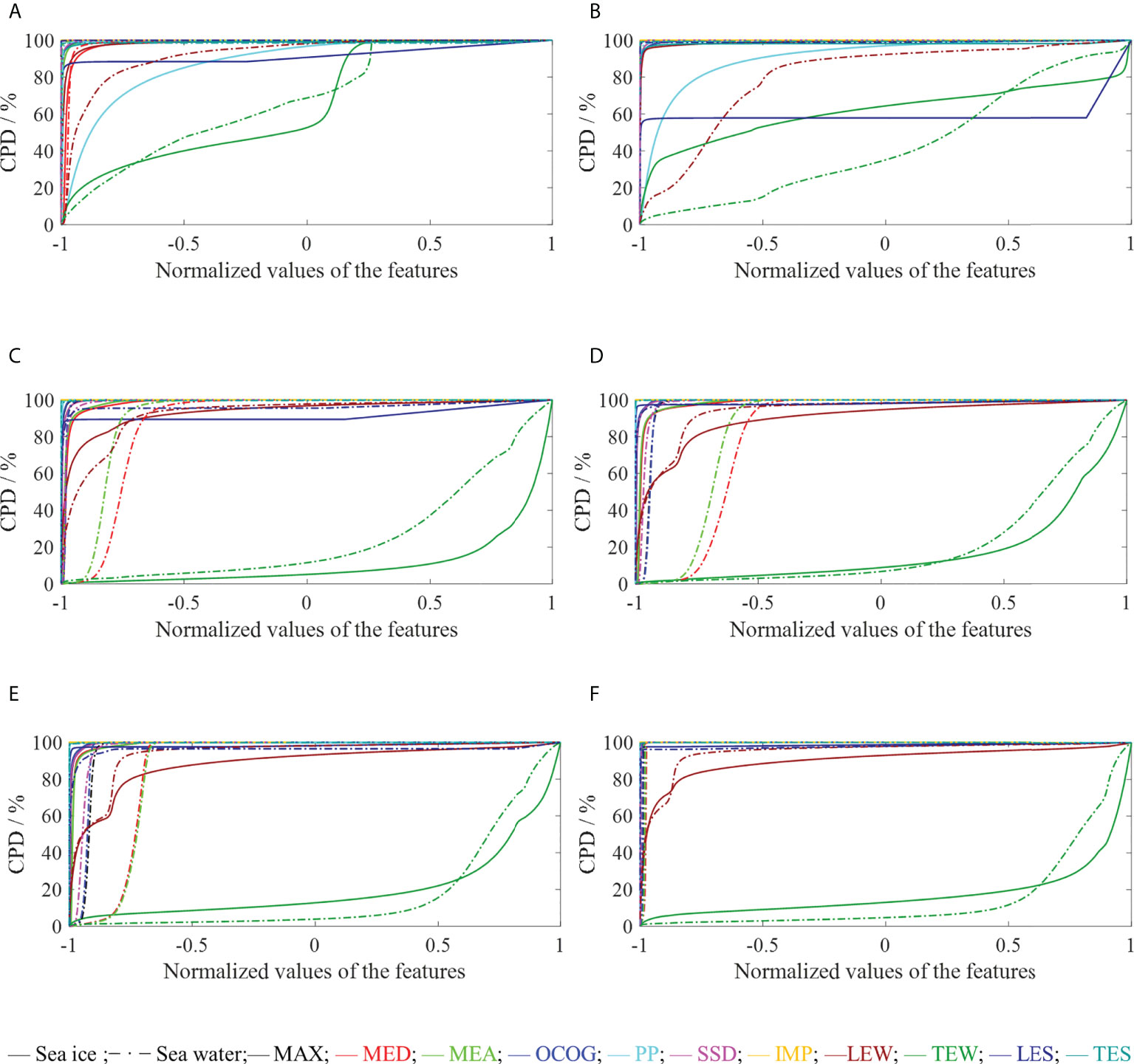
Figure 2 CPDs of eleven features at small incidence angles. (A) 0°; (B) 2°; (C) 4°; (D) 6°; (E) 8°; (F) 10°.

TABLE 1

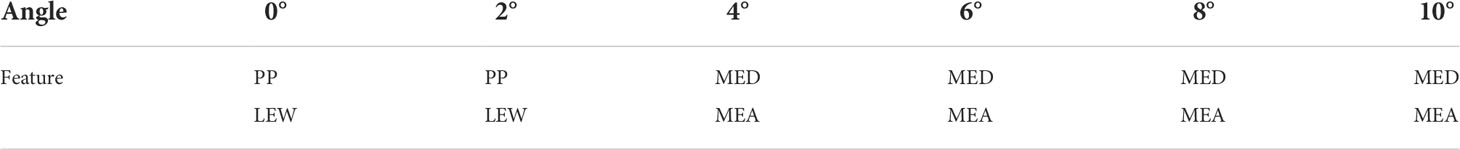
Table 1 The features of which the CPDs obviously differ for sea ice and sea water at six small incidence angles.

3.1.2 MIM

Eleven features can be used to establish 66 feature pairs, and the corresponding MIMs at six small incidence angles are shown in Figure 3. Larger MIMs of feature pairs imply higher redundancy or relevance, and MIMs larger than 0.65 indicate strong correlations (Zhang et al., 2021), as shown in Table 2. At 0–2°, three feature pairs, {OCOG–MAX}, {SSD–MAX} and {SSD–OCOG}, display high redundancy. At 4–6°, {OCOG–MAX} and {MEA–MED} pairs are most strongly correlated. At 8–10°, only the {MEA–MED} pair displays high relevancy. Thus, features at 4–6° may display the characteristics of features at both the 0–2° and 8–10°. More features with less redundancy at 8 – 10° may imply the independence of these features. The MIMs exhibit some consistency with the CPDs; for example, MEA and MED have high relevance and display similar CPD distributions at 4–10°. Consequently, a high MIM value indicates the high repeatability and redundancy of the two features in sea ice and sea water separation.

FIGURE 3

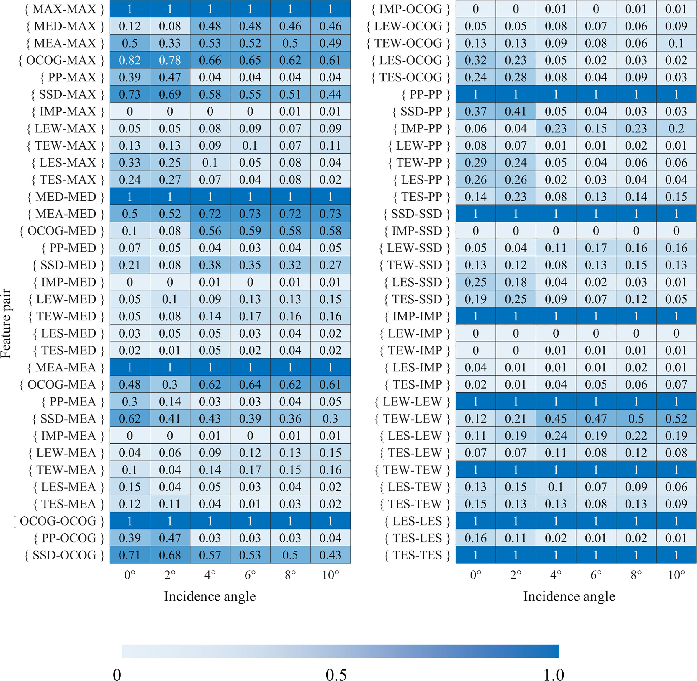
Figure 3 MIMs of 66 feature pairs at small incidence angles.

TABLE 2

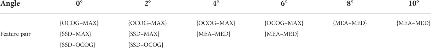
Table 2 The feature pairs of which the MIMs are larger than 0.65 at six small incidence angles.

Considering that no one feature pair appears at all incidence angles, all features are considered in subsequent research.

3.2 Three classifiers

All features are used in the KNN, SVM and RF methods, and the model parameterization results are compared to the above feature analysis results.

3.2.1 RF

The number of decision trees in the RF method is varied from 10–100 with a step of 10, and the overall accuracies of sea ice and sea water are shown in Figure 4A. This subfigure shows that the accuracies are very steady under different conditions of decision trees, features and incidence angles, and the lines of maximum values are often very close to the lines of minimum values. The accuracies decrease very slowly as the number of trees increases, and the maximum change in the accuracies is approximately 1.2%. As a result, more trees do not produce higher accuracy for all features at six small incidence angles, but the run time does notably increase. Thus, the classification results of 10 decision trees (Tree 10) in the RF are compared with the KNN and SVM results.

FIGURE 4

Figure 4 Overall accuracies of the RF method for different tree numbers and the KNN method for different k values at small incidence angles: (A) Different numbers of RF trees: Mean values of the overall accuracies are expressed by the bars; The maximum value and minimum value of the overall accuracies are indicated by two orange short lines on the bar, respectively; The upper line represents the maximum value, and the lower line is the minimum value; (B) Different k values at 0°; (C) Different k values at 2°; (D) Different k values at 4°; (E) Different k values at 6°; (F) Different k values at 8°; (G) Different k values at 10°.

3.2.2 KNN

Two parameters in the KNN method are tested: the k value and distance. The value range of k is set to 1 to 13, and the accuracy of the corresponding results is shown in Figures 4B–G. At all incidence angles, the change in accuracy can reach 17% before k = 5; then, the accuracy change remains at approximately 1.7% (only LEW of 2° is about 6.7%) for k values from 5 to 11, and 1.0% for k values larger than 11. Thus, k is set to 11 in the KNN model.

The three distances (Euclidean distance, Manhattan distance, and Mahalanobis distance) are analyzed, and the results are compared with those of the RF and SVM, as shown in Figure 5. The run time of the model with Euclidean distance is slightly shorter than that of the model based on the Manhattan distance and much shorter than that of the model with the Mahalanobis distance.

FIGURE 5

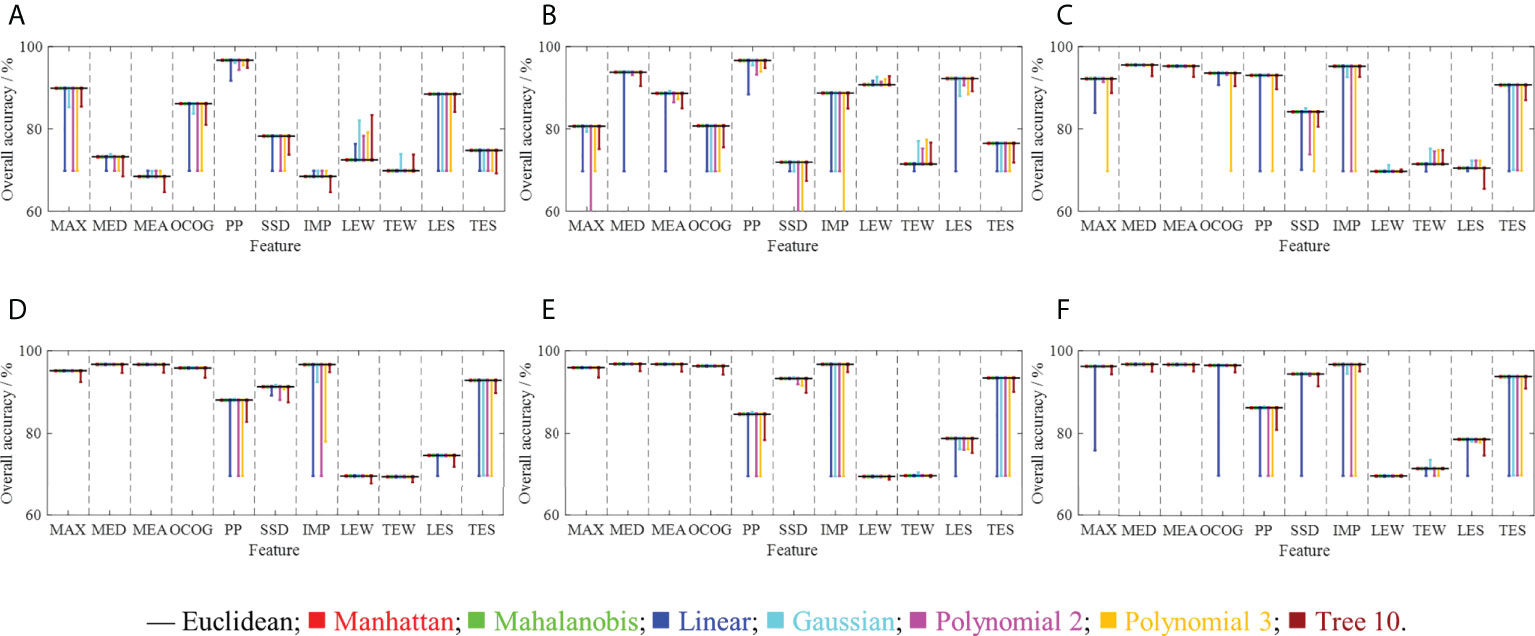
Figure 5 Overall accuracies of the individual RF, KNN and SVM models with different settings: (A) 0°; (B) 2°; (C) 4°; (D) 6°; (E) 8°; (F) 10°. The result of the Euclidean distance is expressed as the solid black line, and the other kernels, distances and Tree 10 are shown as bars based on the Euclidean distance. Upward bars express their accuracies higher than the overall accuracies of the Euclidean distance, and the downward bars express their accuracies less than the overall accuracies of the Euclidean distance.

3.2.3 SVM

The SVM run times with different kernels are as follows in ascending order: linear kernel, Gaussian kernel, polynomial kernel with q equal to 2 (Polynomial 2), and polynomial kernel with q equal to 3 (Polynomial 3). The accuracy results are compared for eight cases, namely, ‘Tree 10’ for the RF with 10 trees, the KNN with k =11 and three different distance measures, and the SVM with three different kernels, as shown in Figure 5.

The overall accuracy results illustrate that the KNN model with Euclidean distance yields better results than the other cases, except for IMP at 0°, LEW and TEW from 0–4°, and LES at 4°. Thus, the optimal classifier is the KNN method with Euclidean distance and k equal to 11. The overall accuracies for single features are shown in Table 3. The top-three features with the highest accuracies at small incidence angles are marked in red.

TABLE 3

Table 3 Overall accuracies of single features at small incidence angles using the optimal classifier (the KNN method with Euclidean distance and k equal to 11).

At 0–2°, PP and LES are common top features, and PP is also noted as a top feature in the CPDs (Section 3.1.1). At 4–6°, the results are similar to those at 8–10°, which is consistent with the CPD results. At 8–10°, higher accuracies are observed than those at other incidence angles. Moreover, at 4–6° and 8–10°, the two incidence sets have the same top-three features (MED, MEA, and IMP); both MED and MEA are effective for sea ice and sea water separation in agreement with their CPDs and MIMs in Section 3.1.

3.3 Optimal classifier-feature assembly

The eleven features can be used to construct 2047 feature combinations at each incidence angle. These feature combinations are input into the optimal classifier, that is, the KNN classifier with Euclidean distance and k = 11; the resulting F1 scores and overall accuracies are shown in Figure 6.

FIGURE 6

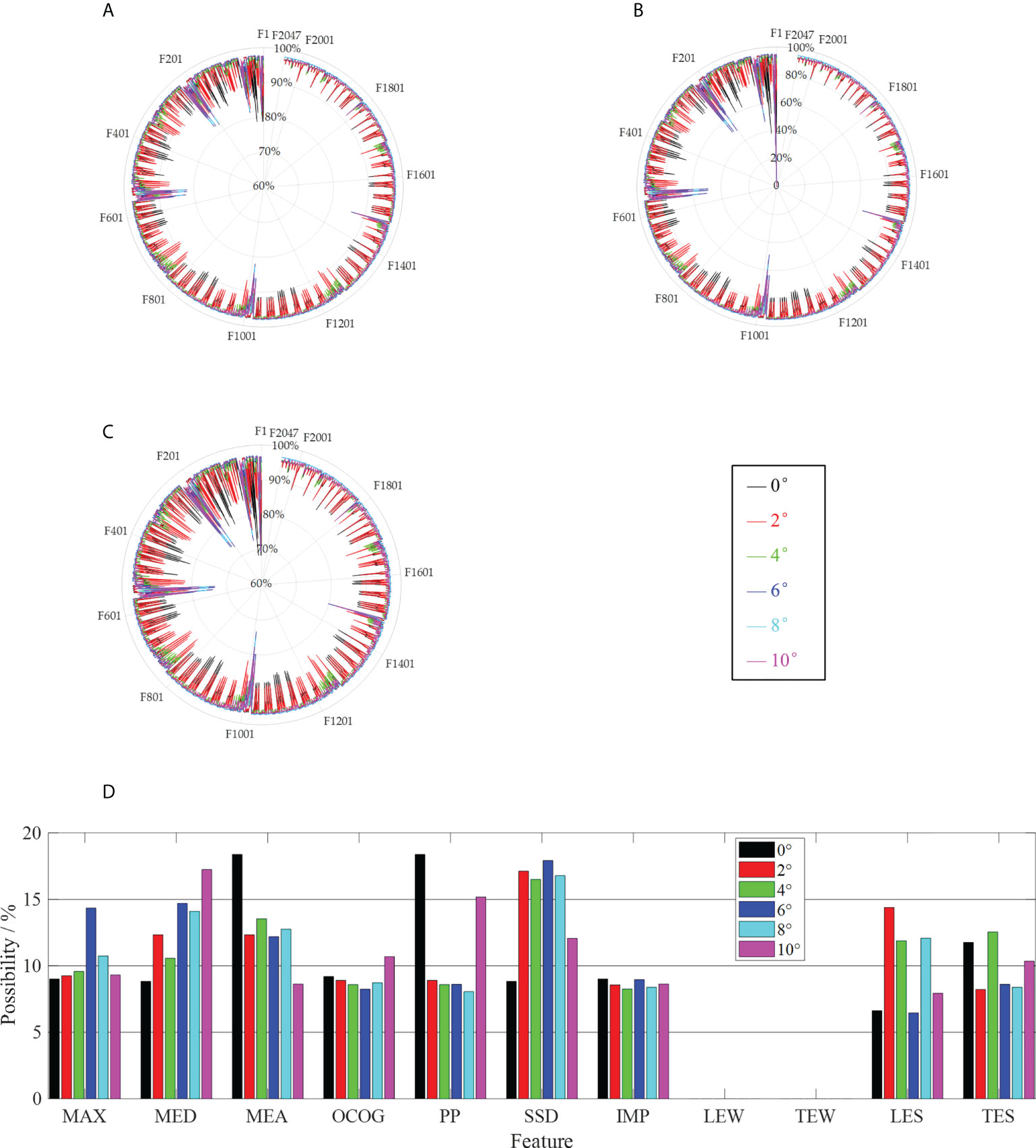
Figure 6 F1 scores and overall accuracies of 2047 feature combinations for sea ice and sea water discrimination at six small incidence angles. (A) F1 scores of sea ice; (B) F1 scores of sea water; (C) Overall accuracies; (D) Occurrence possibilities of single features in the top 5% feature combinations. The numbers in (A) – (C) represent the ID Numbers of the feature combinations, seen in the ‘Supplementary Material’ file.

The optimal feature combination that yields the highest accuracy at each incidence angle is shown in Table 4. The highest overall accuracy reaches 97.1%. There are few identical features in the optimal combinations of each incidence set because of the large number of feature combinations. For different feature combinations, the numbers of overall accuracies better than 96% are 970, 948, 994, 1769, 1879, and 1430 at each incidence angles, respectively. As a result, we focus on not only the optimal feature combinations but also the feature combinations that score in the top-5 percent in terms of overall accuracy. The occurrence probabilities of single features in these top combinations are analyzed, as shown in Figure 6D. The results for 6–10° are better than those at other incidence angles.

TABLE 4

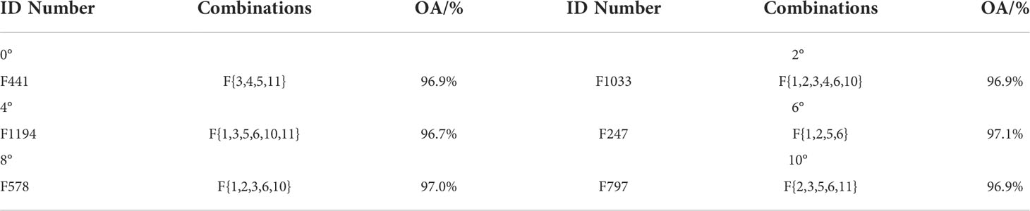
Table 4 Overall accuracy of the optimal feature combination at each small incidence angle using the optimal classifier (the KNN method with Euclidean distance and k equal to 11).

At 0–2°, the optimal/top combinations mainly include MED, MEA, OCOG, PP, SSD, LES and TES (F{2,3,4,5,6,10,11}). PP (F5), as an important feature in altimeter-based sea ice recognition, is common in the top combinations and is high ranking in the above CPDs (Section 3.1.1) and single feature classification results (Section 3.2). OCOG and SSD (F4, F6) are relevant in MIMs, but are still functional in the optimal combination of F1033 at 2°, which implies that the two features can play their own roles for sea ice recognition. At 4–6°, the optimal/top combinations mainly include MAX, MED, MEA, PP, SSD, LES and TES (F{1,2,3,5,6,10,11}). MED and MEA (F2, F3) can also be effectively used to distinguish between sea ice and sea water suggested by CPDs and single feature classification. The two features have high relevance in MIMs, and they are the important features in optimal combinations of F1194 at 4° and F247 at 6°, respectively. At 8–10°, the optimal/top combinations mainly include MAX, MED, MEA, PP, SSD, LES and TES (F{1,2,3,5,6,10,11}). MED and MEA (F2, F3) are very useful to discriminate sea ice and sea water indicated by CPDs and single feature classification. MED and MEA are redundant in MIMs and provide respective contributions in the optimal combinations of F578 at 8° and F797 at 10°. MEA performs better than OCOG for 4° to 10°, which indicates that MEA may be more suitable to express σ₀ for 4° to 10°. The results at 4–6° are similar to those at 8–10°, as observed in the CPDs and single feature classification.

According to the above results, angles from 6° to 10° are best for distinguishing between sea ice and sea water. The top feature combinations display obvious consistency with the relevant CPD results and single feature classification results. Moreover, these results are in partial agreement with MIM analysis results. Nevertheless, some features in redundant or relevant feature pairs can play their own functions for sea ice and sea water discrimination in the optimal combination. Therefore, optimal classifier–feature assembly at each incidence angle can be used for sea ice recognition based on SWIM data.

3.4 Application analysis of optimal classer-feature assembly

3.4.1 Sea ice recognition accuracies in three stages of sea ice development

The three stages of sea ice development in the Arctic ice year of 2020/2021 are expressed specifically by combining the AARI and NSIDC sea ice charts as follows. The first stage is from 4^th to 27^th October, 2020 (Stage 1), when the sea ice changed clearly. The second stage is from 1^st November to 29^th December, 2020 (Stage 2), when the sea ice grew rapidly. The third stage is from 3^rd January to 27^th April, 2021 (Stage 3), when the sea ice distribution was stable. Several regions where sea ice and sea water do not vary throughout each stage are selected according to sea ice charts in the three stages. The selected invariant regions of the categories for Stages 1–3 are as large as possible, as shown in Figure 7.

FIGURE 7

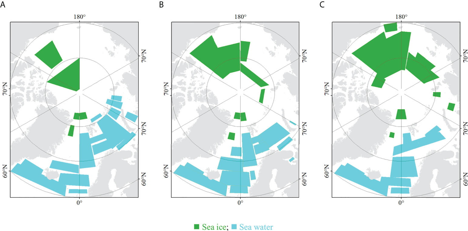
Figure 7 Invariant regions of the sea ice distribution at each stage: (A) Stage 1; (B) Stage 2; (C) Stage 3.

For each stage, five time intervals of one day (T1), three days (T2), one week (T3), one month (T4) and one stage (T5) are selected, and T4 and T5 are the same in Stage 1. The overall accuracies are shown in Table 5.

TABLE 5

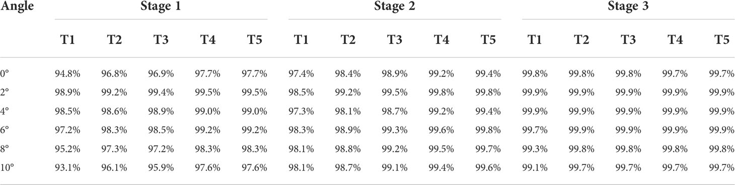
Table 5 The overall accuracies for Stages 1–3 using the optimal classifier–feature assembly at each small incidence angle.

In the three stages, the overall accuracies of the optimal assemblies at small incidence angles in T1–T5 are higher than 90%. In addition, the accuracy generally increases as sea ice development stabilizes. Moreover, the excellent accuracies may be partly due to homogeneous characteristics in these areas where boundary regions of sea ice and sea water are not included. Therefore, optimal classifier–feature assemblies can be effectively used for sea ice and sea water separation at all incidence angles in short- and long-term periods.

3.4.2 Sea ice extent and edge extraction

The sea ice recognition results based on SWIM data can be applied to detect sea ice extents and edges. According to the SWIM coverage, seven-day data are merged to build a grid image with a resolution of 25 km × 25 km in the polar stereographic projection, consistent with NSIDC sea ice products for the Arctic. In one grid, the sea ice proportion can be calculated based on the number of sea ice footprints divided by the total numbers of sea ice and sea water footprints. The grids where the sea ice proportion is not lower than 15% are set to sea ice regions, and others are sea water regions; then, sea ice extents and edges can be identified. Three SWIM results of sea ice extents and edges, combining synchronous Sentinel-1 SAR images from the ice year of 2020/2021, are used as examples to assess the proposed approach during November 11^th – 17^th, 2020, February 11^th – 17^th, 2021, and March 11^th – 17^th, 2021. Additionally, these results are also compared with the NSIDC sea ice products. The time difference between the acquisitions of the Sentinel-1 SAR images and the release of the AARI sea ice charts or the NSIDC products is less than 1 day. And, when SWIM results are evaluated by a SAR image, these results should be obtained on one day (SR-1). Then, the time difference between the acquisitions of the SAR image and SWIM data is less than 1 day. Comparison of sea ice extents and edges between SWIM and NSIDC are shown in Figure 8. For each grid, the type of SWIM (in seven days, SR-7) and NSIDC (in one day, NR-1) are compared, then the percentage of the grids with the same type (sea ice or water) is found to be 94.8% (SR-7 from November 11^th – 17^th, and SAR and NR-1 on November 11^th), 97.7% (SR-7 from February 11^th – 17^th, and SAR and NR-1 on February 17^th), and 98.2% (SR-7 from March 11^th – 17^th, and SAR and NR-1 on March 17^th), respectively. These results reveal that SWIM sea ice extents are consistent with those of NSIDC.

FIGURE 8

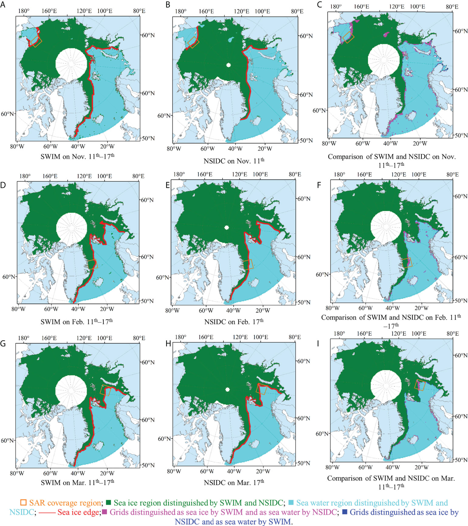
Figure 8 Comparison of sea ice extents and edges between SWIM and NSIDC. (A) SWIM on Nov. 11^th – 17^th; (B) NSIDC on Nov. 11^th; (C) Comparison of SWIM and NSIDC on Nov. 11^th – 17^th; (D) SWIM on Feb. 11^th – 17^th; (E) NSIDC on Feb. 17^th; (F) Comparison of SWIM and NSIDC on Feb. 11^th – 17^th; (G) SWIM on Mar. 11^th – 17^th; (H) NSIDC on Mar. 17^th; (I) Comparison of SWIM and NSIDC on Mar. 11^th – 17^th.

The obvious differences of sea ice extents between SWIM and NSIDC mainly occur in coastal areas and sea ice edges. In the coastal areas, the land information can influence the results of sea ice recognition, and in sea ice edges, the confusion of sea ice and sea water may also affect the results. The differences in the sea ice edges are studied combining synchronous Sentinel-1 SAR images. And in order to clearly reveal these differences, only the sea ice edges of overlapping regions of NR-1 and SR-7 or SR-1 are shown in Figure 9.

FIGURE 9

Figure 9 Sea ice edges based on SWIM and NSIDC data with synchronous Sentinel-1 SAR images. (A) Sentinel-1 SAR image, HV, at 18:04:46, Nov. 11^th; (B) Sea ice region of NSIDC on Nov. 11^th; (C) Sea ice region of NSIDC on Nov. 14^th; (D) Sea ice region of NSIDC on Nov. 17^th; (E) Sea ice region of SWIM on Nov. 11^th – 17^th; (F) Sentinel-1 image and SWIM data on Nov. 11^th; (G) Sea ice region of SWIM on Nov. 11^th; (H) Sea ice edge on Nov. 11^th – 17^th; (I) Sentinel-1 SAR image, HV, at 07:55:48, Feb. 17^th; (J) Sea ice region of SWIM on Feb. 17^th; (K) Sea ice region of NSIDC on Feb. 17^th; (L) Sea ice edge on Feb. 17^th; (M) Sentinel-1 SAR image, HV, at 04:04:26, Mar. 17^th; (N) Sea ice region of SWIM on Mar. 17^th; (O) Sea ice region of NSIDC on Mar. 17^th; (P) Sea ice edge on Mar. 17^th.

From November 11^th – 17^th, the SWIM sea ice edges are matched with the Sentinel-1 SAR image obtained on November 11^th. A comparison of the sea ice edges in the SWIM and NSIDC products with the Sentinel-1 image indicates that the sea ice distribution is overestimated in SR-7 and NR-1 products, and the result of SR-7 is worse than that of NR-1, as shown by the blue line and purple line in Figure 9H. Considering that sea ice developed rapidly in November, SR-1 on November 11^th is chosen to build grids (Figure 9F–G), and many blank grids (no data) appear; then, only regions with data are analyzed. The sea ice edge of SR-1 product agrees with the Sentinel-1 image, which is more accurate than NR-1 results. However, there is still one grid incorrectly labeled as sea ice in SR-1 result. From February 11^th – 17^th, sea ice edges of SR-1 are matched with the Sentinel-1 SAR image obtained on February 17^th. Sea ice regions are overestimated in the NR-1 product, and slightly underestimated in the SR-1 product. The sea ice edge result of SR-1 is a bit better than that of NR-1. From March 11^th – 17^th, the SWIM sea ice edges are matched with the Sentinel-1 SAR image obtained on March 17^th. The lead in the top left corner of the Sentinel-1 image is marked with a red line. In this area, the sea ice edges in the NR-1 product are more accurate than those in the SR-1 product, and occur a little underestimated. The misjudged regions in the SR-1 product are approximately the width of 2–3 grids and may be due to multiple categories in one footprint. Below the lead, compared with SR-1 results, the sea ice edges in the NR-1 product are misjudged in some grids. Therefore, for sea ice extents, the SWIM results are more consistent with the NSIDC results in the stable sea ice stage. Moreover, the sea ice edges in the SR-1 product are precise. SWIM can be a new data source to generate practical sea ice products.

4 Discussion

Our study mainly focuses on two objectives: the development of a sea ice recognition method for the new SWIM observation mode and the application of SWIM data using optimal classifier–feature assemblies.

4.1 Development of sea ice recognition method

The six small incidence angles are divided into three sets according to the analysis of CPDs and MIMs, and these incidence sets exhibit distinct characteristics for sea ice recognition. The results at 4–6° encompass characteristics of those at 0–2° and 8–10° and coincide better with the results at 8–10°. For single feature classification, IMP and TES in our previous work were only used to separate FYI and MYI; whereas, in this study, they are adopted for sea ice and sea water separation, and the related feature LES is also used. In the previous work, the OCOG was used for 0° and MEA for 2–10°; whereas, in this study, both of them are used for all incidence angles. MED is a new feature, and is rarely introduced in other studies. At 0–2°, PP is the best feature, as previously reported for altimeter-based methods (Rinne and Similä, 2016; Paul et al., 2018; Jiang et al., 2019; Aldenhoff et al., 2019). From 4–10°, MEA, which reflects the properties of σ₀, highly enhances sea ice and water separation in conjunction with scatterometer and SAR data (Otosaka et al., 2018; Zhang et al., 2019). Because LES and TES combine the properties of LEW and TEW with MAX, they yield higher accuracies than LEW and TEW in sea ice separation in agreement with our previous work (Liu et al., 2022). Although IMP is used in altimeter-based methods at 0° (Aldenhoff et al., 2019), it is also important from 4–10°. MED, not only reveals some of the characteristics of MAX but also describes the distribution properties of echo waveforms, and it yields excellent results from 2–10°. In general, the newly introduced MED, LES and TES features are valuable for sea ice recognition.

The main features in the optimal/top feature combinations at 0–2° are MED, MEA, OCOG, PP, SSD, LES and TES, agreeing with the results of previous studies. Drinkwater (1991) suggested that altimeters were sensitive to sea ice and that sea ice could be detected based on waveform features such as pulse width (similar to LEW plus TEW), PP and σ₀ based on studies with a Ku-band airborne radar altimeter. Rinne and Similä (2016) reported classification accuracies of 87–92% for sea water and 31–97% for sea ice in three periods using the KNN method with PP, SSD, LEW, and LES based on Cryosat-2. Shen et al. 2017a; Shen et al., 2017b;) obtained a maximum accuracy of 96.6% for sea ice and 95.1% for sea water with an RF classifier using σ₀, MAX, PP, SSD, LEW, and TEW. Shu et al. (2019) distinguished between sea ice and sea water using an RF classifier with PP, LEW, TEW, SSD, MAX, and σ₀ and obtained accuracies above 95%. Müller et al. (2017) investigated Arctic areas using KNN and K-medoids classifiers with waveform features such as MAX and achieved accuracies up to 94%. Jiang et al. (2019) separated sea ice and sea water using KNN and SVM classifiers with wave features such as the PP of Haiyang-2 A/B, and their accuracies were approximately 80%. Thus, the classification accuracies in this study are better than those previously reported, which may be due to the using of more waveform features and the new feature (MED) at multiple small incidence angles in this paper.

The analysis of optimal/top feature combinations is consistent with that of the CPDs and it is partly consistent with that of the MIMs. Moreover, some feature pairs display high redundancy or relevance but play important roles in the optimal combination. The redundancy or relevance of features does not largely affect the performance of sea ice recognition using feature combinations. Therefore, sea ice and sea water recognition can be performed with high accuracy using the proposed optimal classifier–feature assemblies at small incidence angles. Moreover, our results are consistent with those of previous studies and indicate better effects.

4.2 Application of the optimal classifier–feature assemblies

The overall accuracies of sea ice recognition using the optimal classifier–feature assemblies in Stages 1–3 are higher than 90 percent. Sea ice development obviously affects the accuracy of the proposed approach. The invariant distribution of sea ice contributes to high overall accuracy. As a result, the optimal classifier–feature assembly can be used to provide sea ice recognition results with high accuracy, and sea ice can then be removed from SWIM sea wave products. Moreover, SWIM can be a valid data source for operational sea ice monitoring.

According to the sea ice recognition results based on SWIM data, sea ice extents and edges can be extracted and compared with Sentinel-1 SAR images and NSIDC sea ice products. SWIM sea ice extents are consistent with those of NSIDC at a high level of precision. And, SWIM provides a good one-day product of sea ice edges. In this study, the threshold of the sea ice proportion is 15 percent, following the common threshold used for sea ice recognition. However, one SWIM footprint may consist of both sea ice and sea water. In addition, areas with sea ice–water mixing can generate complex waveform signals (March 17^th, 2021, Figure 9P), and a fixed proportional threshold of sea ice and sea water is not appropriate. As a result, the threshold for SWIM data should be further studied. The sea ice edges on March 17^th are used as examples to analyze the threshold, and the thresholds are set as 40%, 50%, and 60%, as shown in Figure 10. Sea ice regions evidently decrease with increasing threshold, and the threshold of 50% is most suitable for sea ice edge extraction on March 17^th, especially for the lead. Thus, the threshold of 15% is not appropriate for all situations. In future work, the threshold selection should be studied; for example, the sea ice distribution and its development stage should be considered. In addition, the probability that one SWIM footprint is classified to sea ice or sea water using the optimal classifier–feature assembly is extracted. As a result, one footprint is not simply judged to sea ice or sea water. The probability is used to calculate the sea ice proportion of one grid, which may improve its accuracies.

FIGURE 10

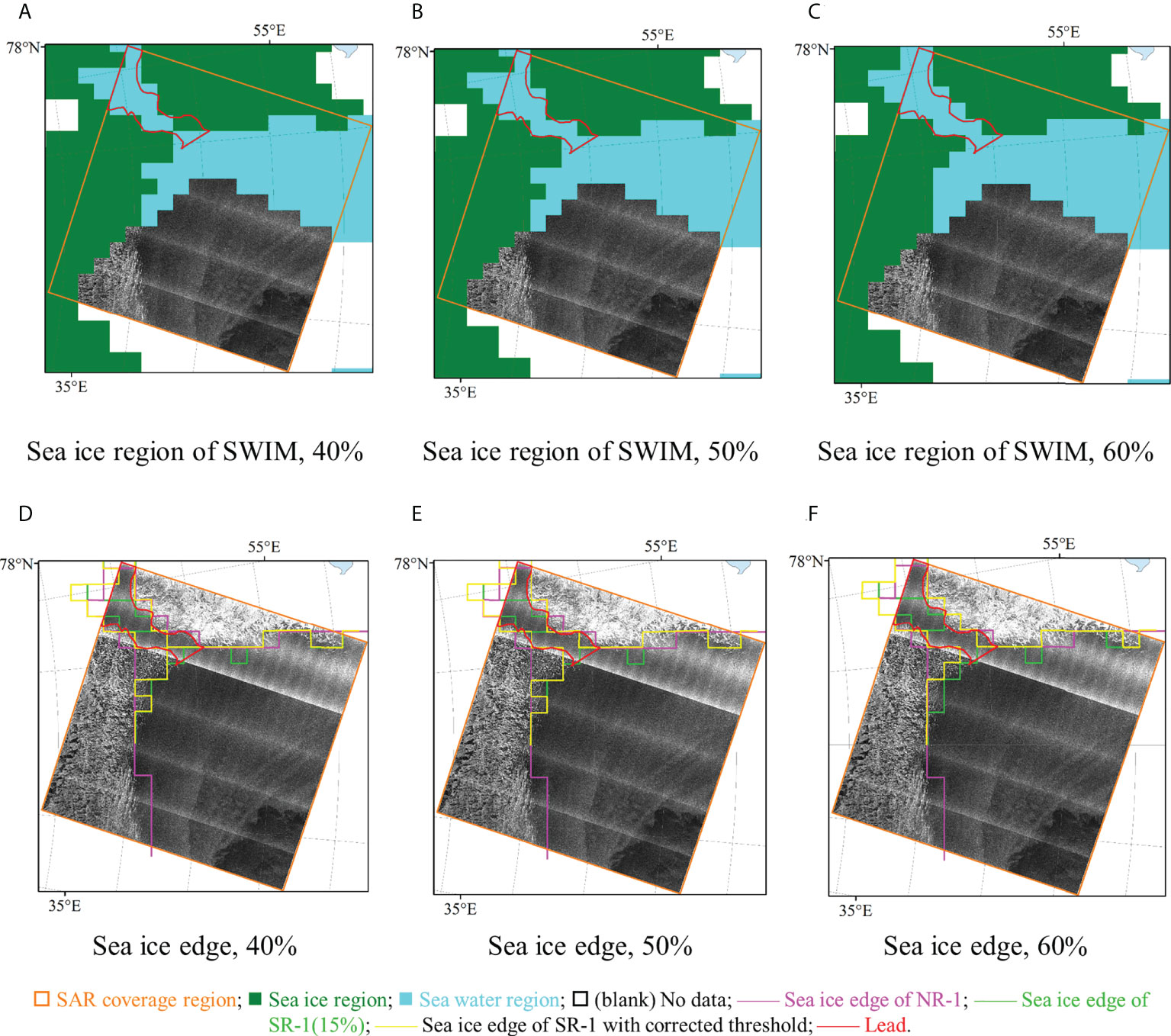
Figure 10 Sea ice edges based on SWIM data with different thresholds of the sea ice proportion. (A) Sea ice region of SWIM, 40%; (B) Sea ice region of SWIM, 50%; (C) Sea ice region of SWIM, 60%; (D) Sea ice edges, 40%; (E) Sea ice edges, 50%; (F) Sea ice edges, 60%.

The results of sea ice recognition in this study are compared to those of sea ice classification in our previous study, and the optimal classifier–feature assemblies at all incidence angles proposed here yield better results. Therefore, sea ice recognition can be accurately performed with the optimal classifier–feature assemblies at small incidence angles in the short- and long-term periods. And, the optimal classifier–feature assemblies can satisfy the sea ice removal requirements for SWIM products, and improve sea ice extent and edge products. In order to further verify the optimal classifier–feature assemblies, more sea ice charts should be introduced, for example, sea ice products of Canadian Ice Service and the University of Bremen (Shi et al., 2020; Komarov and Buehner, 2021). Moreover, new validation methods are also considered for multiple sea ice charts (Wang J. et al., 2021). Our work can fill the gap of sea ice recognition at the multiple small incidence angles, then, achieve the sea ice recognition at normal-, small- and mid-incidence angles.

5 Conclusion

SWIM, as a new type of microwave remote sensor at multiple incidence angles, has been rarely used for sea ice recognition. The main objectives of this study are to develop a sea ice recognition method based on SWIM data with a new observation mode and assess the application of the proposal method, including waveform feature analysis, optimal classifier–feature assembly construction (classifier selection and parameter setting, and feature combination selection), and the assembly application.

(1) Waveform feature analysis

Eleven waveform features of SWIM data in the Arctic from October 2020 to April 2021 are extracted. CPDs and MIMs are used to analyze the characteristics of these waveform features. The results reveal that incidence angles can be divided into three sets at 0–2°, 4–6° and 8–10°. These incidence sets display unique distribution ranges and probabilities for each feature, and the redundancy or relevance of each feature pair is evaluated.

(2) Optimal classifier–feature assembly construction

The RF, KNN and SVM classifiers are explored, and their parameters are set according to the overall accuracies obtained for single features. The KNN classifier with Euclidean distance and k equal to 11 yields the optimal result. Then, feature combinations with the KNN method are used to separate sea ice and sea water and build the optimal classifier-feature assembly for each small incidence angle. The results illustrate that the highest overall accuracy at each incidence angle is greater than 96% and can reach 97.1%. The newly introduced features in this study, such as MED, perform very well.

(3) Optimal classifier–feature assembly application

The application of the optimal classifier–feature assemblies is analyzed. On the one hand, the optimal assemblies are used to distinguish between the sea ice and sea water in different growing stages, and the accuracies are higher than 93.1%, and can reach 99.9%. Then, the results can meet the requirements for SWIM-based sea wave retrieval. On the other hand, sea ice extents can be extracted from these SWIM results with high accuracies that are higher than 94.8% and up to 98.2%, and SWIM provides a better one-day product of sea ice edges than the NSIDC product. The results indicate that SWIM can provide new data for operational sea ice monitoring. Our results are also compared with those of other studies and indicate better effects and consistency.

In conclusion, in this study, a sea ice recognition method using optimal classifier–feature assemblies is proposed, and it can not only perform sea ice recognition with high accuracy using new-mode SWIM data but also provide discrimination flags of sea ice in SWIM products. Moreover, our research on the application of the proposal method can reliably provide sea ice extent and edge products, then SWIM data can be used as a new data source for operational sea ice monitoring.

In future work, more SWIM data from different ice years will be used to verify the validity and robustness of the classifier–feature assemblies. And, other classifiers, such as Bayesian, convolutional neural network and propagation neural network classifiers, will be studied to potentially improve sea ice recognition. Moreover, more sea ice products such as the sea ice concentration and types will be further studied in conjunction with SWIM data.

Data availability statement

The original contributions presented in the study are included in the article/Supplementary Material. Further inquiries can be directed to the corresponding author.

Author contributions

ML made most of analysis and wrote the main manuscript. RY and XZi made interpretation and discussion of the results. PC and YX reviewed the manuscript. YZ, YG, YC, XZia, SL undertook the data processing. All authors made important contributions to the contents of the paper. All authors have revised and approved the manuscript.

Funding

This research was funded in part by the Shandong Provincial Natural Science Foundation, China under grant ZR2019MD016; the National Natural Science Foundation of China under grant 41976173, 61971455, and 41976168; the Shandong Provincial Natural Science Foundation, China under grant ZR2020MD095, ZR201910290171; the Shandong joint fund of National Natural Science Foundation of China under grant U2006207; and the Ministry of Science and Technology of China and the European Space Agency through the Dragon-5 Program under grant 57889.

Acknowledgments

Sea ice recognition was based on the SWIM. SWIM data of CFOSAT were obtained from https://osdds.nsoas.org.cn. The authors would like to thank NSOAS for providing the data free of charge. Sea ice charts were provided by the AARI and NSIDC. The accuracy evaluation of sea ice recognition was supported partly by Sentinel-1 SAR data. The publication is supported by the University-Industry Joint Center for Ocean Observation and Broadband Communication.

Conflict of interest

The authors declare that the research was conducted in the absence of any commercial or financial relationships that could be construed as a potential conflict of interest.

Publisher’s note

All claims expressed in this article are solely those of the authors and do not necessarily represent those of their affiliated organizations, or those of the publisher, the editors and the reviewers. Any product that may be evaluated in this article, or claim that may be made by its manufacturer, is not guaranteed or endorsed by the publisher.

Supplementary material

The Supplementary Material for this article can be found online at: https://www.frontiersin.org/articles/10.3389/fmars.2022.986228/full#supplementary-material

References

Aldenhoff W., Heuzé C., Eriksson L. E. B. (2019). Sensitivity of radar altimeter waveform to changes in Sea ice type at resolution of synthetic aperture radar. Remote Sens. 11, 2602. doi: 10.3390/rs11222602

CrossRef Full Text | Google Scholar

Arctic and Antarctic Research Institute (2022) AARI. Available at: http://www.aari.ru/ (Accessed 2022).

Google Scholar

Asadi N., Scott K. A., Komarov A. S., Buehner M., Clausi D. A. (2021). Evaluation of a neural network with uncertainty for detection of ice and water in SAR imagery. IEEE Trans. Geosci. Remote Sensing. 59, 247–259. doi: 10.1109/TGRS.2020.2992454

CrossRef Full Text | Google Scholar

Berg A., Eriksson L. E. (2012). SAR algorithm for sea ice concentration–evaluation for the Baltic Sea. IEEE Geosci. Remote Sens. Lett. 9 (5), 938–942. doi: 10.1109/LGRS.2012.2186280

CrossRef Full Text | Google Scholar

Bi H., Zhang J., Wang Y., Zhang Z., Zhang Y., Fu M., et al. (2018). Arctic Sea Ice volume changes in terms of age as revealed from satellite observations. IEEE J. Sel. Top. Appl. Earth Obs. Remote Sens. 11, 1–15. doi: 10.1109/JSTARS.2018.2823735

CrossRef Full Text | Google Scholar

Breivik L. A., Eastwood S., Lavergne T. (2012). Use of c-band scatterometer for Sea ice edge identification. IEEE Trans. Geosci. Remote Sens. 50, 2669–2677. doi: 10.1109/TGRS.2012.2188898

CrossRef Full Text | Google Scholar

Cavalieri D. J., Parkinson C., Gloersen P., Zwally H., Meier W., Fetterer F., et al. (1996). Data from: Sea ice concentrations from nimbus-7 SMMR and DMSP SSM/I-SSMIS passive microwave data, version 1 (University of Colorado Boulder: NSIDC). Available at: https://nsidc.org/data/NSIDC-0051/versions/1.

Google Scholar

Chan C. W., Paelinckx D. (2008). Evaluation of random forest and adaboost tree-based ensemble classification and spectral band selection for ecotope mapping using airborne hyperspectral imagery. Remote Sens. Environment. 112, 2999–3011. doi: 10.1016/j.rse.2008.02.011

CrossRef Full Text | Google Scholar

Cheng A., Casati B., Tivy A., Zagon T., Lemieux J. F., Tremblay L. B. (2020). Accuracy and inter-analyst agreement of visually estimated sea ice concentrations in Canadian ice service ice charts using single-polarization RADARSAT-2. Cryosphere. 14, 1289–1310. doi: 10.5194/tc-14-1289-2020

CrossRef Full Text | Google Scholar

de Gélis I., Colin A., Longepe N. (2021). Prediction of categorized sea ice concentration from sentinel-1 SAR images based on a fully convolutional network. IEEE J. Selected Topics Appl. Earth Observat. Remote Sens. 14, 5831–5841. doi: 10.1109/JSTARS.2021.3074068

CrossRef Full Text | Google Scholar

Drinkwater M. R. (1991). Kuband airborne radar altimeter observations of marginal sea ice during the 1984 marginal ice zone experiment. J. Geophys. Res. 96, 4555. doi: 10.1029/90jc01954

CrossRef Full Text | Google Scholar

Drinkwater M. R., Carsey F. D. (1991). Observations of the late-summer to fall sea ice transition with the 14.6 GHz seasat scat-terometer. IEEE 3, 1597–1600. doi: 10.1109/IGARSS.1991.579499

CrossRef Full Text | Google Scholar

Gohin F., Cavanie A. (1994). A first try at identification of sea ice using the three beam scatterometer of ERS-1. Int. J. Remote Sensing. 15, 1221–1228. doi: 10.1080/01431169408954156

CrossRef Full Text | Google Scholar

Haarpaintner J., Spreen G. (2007). Use of enhanced-resolution QuikSCAT/SeaWinds data for operational ice services and climate research: Sea ice edge, type, concentration, and drift. IEEE Trans. Geosci. Remote Sens. 45 (10), 3131–3137. doi: 10.1109/TGRS.2007.895419

CrossRef Full Text | Google Scholar

Hauser D., Tison C., Amiot T., Delaye L., Corcoral N., Castillan P. (2017). Swim: The first spaceborne wave scatterometer. IEEE Trans. Geosci. Remote Sens. 55, 3000–3014. doi: 10.1109/TGRS.2017.2658672

CrossRef Full Text | Google Scholar

Hauser D., Tison C., Amiot T., Delaye L., Mouche A., Guitton G., et al. (2016). “CFOSAT: A new Chinese-French satellite for joint observations of ocean wind vector and directional spectra of ocean waves,” in Remote Sens. Ocean. Inland Wa-ters Tech. Appl. Chall. . (New Delhi, India: SPIE Asia-Pacific Remote Sensing) 9878, 1–20. doi: 10.1117/12.2225619

CrossRef Full Text | Google Scholar

Hauser D., Tourain C., Hermozo L., Alraddawi D., Tran N. T. (2020). New observations from the swim radar on-board cfosat: Instrument validation and ocean wave measurement assessment. IEEE Trans. Geosci. Remote Sens. 59, 5–26. doi: 10.1109/TGRS.2020.2994372

CrossRef Full Text | Google Scholar

Hoekstra M., Jiang M., Clausi D. A., Duguay C. (2020). Lake ice-water classification of RADARSAT-2 images by integrating IRGS segmentation with pixel-based random forest labeling. Remote Sensing. 12, 1425. doi: 10.3390/rs12091425

CrossRef Full Text | Google Scholar

Jiang C., Lin M., Wei H. (2019). A study of the technology used to distinguish Sea ice and seawater on the haiyang-2A/B (HY-2A/B) altimeter data. Remote Sens. 11, 1490. doi: 10.3390/rs11121490

CrossRef Full Text | Google Scholar

Karvonen J., Simila M., Makynen M. J. I. G. (2005). Open water detection from Baltic Sea ice radarsat-1 SAR imagery. IEEE Geosci. Remote Sens. Lett. 2, 275–279. doi: 10.1109/LGRS.2005.847930

CrossRef Full Text | Google Scholar

Komarov A. S., Buehner M. (2021). Ice concentration from dual-polarization SAR images using ice and water retrievals at multiple spatial scales. IEEE Trans. Geosci. Remote Sens. 59 (2), 950–961. doi: 10.1109/TGRS.2020.3000672

CrossRef Full Text | Google Scholar

Laxon S. (1994). Sea Ice extent mapping using the ERS-1 radar altimeter. EARSeL Adv. Remote Sens 3, 112–116.

Google Scholar

Li X. M., Sun Y., Zhang Q. (2021). Extraction of sea ice cover by sentinel-1 SAR based on support vector machine with unsupervised generation of training data. IEEE Trans. Geosci. Remote Sens. 59 (4), 3040–3053. doi: 10.1109/TGRS.2020.3007789

CrossRef Full Text | Google Scholar

Liu H., Guo H., Zhang L. (2015). SVM-based sea ice classification using textural features and concentration from RADARSAT-2 dual-pol ScanSAR data. IEEE J. Selected Topics Appl. Earth Observat. Remote Sensing. 8 (4), 1601–1613. doi: 10.1109/JSTARS.2014.2365215

CrossRef Full Text | Google Scholar

Liu M., Yan R., Zhang J., Xu Y., Chen P., Shi L., et al. (2022). Arctic Sea Ice classification based on CFOSAT SWIM data at multiple small incidence angles. Remote Sensing. 14 (1), 91. doi: 10.3390/rs14010091

CrossRef Full Text | Google Scholar

Liu M., Zhang X., Chen P., Wang J., Zhong S. (2021). “Arctic Sea-Ice type recognition based on the surface wave investigation and monitoring instrument of the China-French ocean satellite,” in In 2021 Photonics & Electromagnetics Research Symposium (PIERS). (Hangzhou, China: IEEE). 2362–2369. doi: 10.1109/PIERS53385.2021.9695052

CrossRef Full Text | Google Scholar

Müller F. L., Dettmering D., Bosch W., Seitz F. (2017). Monitoring the Arctic seas: How satellite altimetry can be used to detect open water in Sea-ice regions. Remote Sens. 9, 551. doi: 10.3390/rs9060551

CrossRef Full Text | Google Scholar

National Snow and Ice Data Center (2022) NSIDC. Available at: https://nsidc.org/data/NSIDC-0051/versions/1.

Google Scholar

Otosaka I., Rivas M. B., Stoffelen A. (2018). Bayesian Sea Ice detection with the ERS scatterometer and sea ice backscatter model at c-band. IEEE Trans. Geosci. Remote Sensing. 56, 2248–2254. doi: 10.1109/TGRS.2017.2777670

CrossRef Full Text | Google Scholar

Paul S., Hendricks S., Ricker R., Kern S., Rinne E. (2018). Empirical parametrization of envisat freeboard retrieval of Arctic and Antarctic sea ice based on CryoSat-2: Progress in the ESA climate change initiative. Cryosphere. 12 (7), 2437–2460. doi: 10.5194/tc-12-2437-2018

CrossRef Full Text | Google Scholar

Remund Q. P., Long D. G. (1999). Sea-Ice extent mapping using Ku-band scatterometer data. J. Geophys. Res. Ocean. 104, 11515–11527. doi: 10.1029/98JC02373

CrossRef Full Text | Google Scholar

Remund Q. P., Long D. G. (2014). A decade of QuikSCAT scatterometer Sea ice extent data. IEEE Trans. Geosci. Remote Sens. 52, 4281–4290. doi: 10.1109/TGRS.2013.2281056

CrossRef Full Text | Google Scholar

Ren L., Yang J., Xu Y., Zhang Y., Zheng G., Wang J., et al. (2021). Ocean surface wind speed dependence and retrieval from off-nadir CFOSAT SWIM data. Earth Space Sci. 8 (6), e2020EA001505. doi: 10.1029/2020EA001505

CrossRef Full Text | Google Scholar

Rinne E., Similä M. (2016). Utilisation of CryoSat-2 SAR altimeter in operational ice charting. Cryosphere 10, 121–131. doi: 10.5194/tc-10-121-2016

CrossRef Full Text | Google Scholar

Rivas M. B., Stoffelen A. (2011). New Bayesian algorithm for sea ice detection with QuikSCAT. IEEE Trans. Geosci. Remote Sens. 49 (6), 1894–1901. doi: 10.1109/TGRS.2010.2101608

CrossRef Full Text | Google Scholar

Rivas M. B., Verspeek J., Verhoef A., Stoffelen A. (2012). Bayesian Sea Ice detection with the advanced scatterometer ASCAT. IEEE Trans. Geosci. Remote Sens. 50, 2649–2657. doi: 10.1109/TGRS.2011.2182356

CrossRef Full Text | Google Scholar

Scharien R. K., Nasonova S. (2022). Incidence angle dependence of texture statistics from sentinel-1 HH-polarization images of winter Arctic Sea ice. IEEE Geosci. Remote Sens. Lett. 19, 1–5. doi: 10.1109/LGRS.2020.3039739

CrossRef Full Text | Google Scholar

Shen X., Jie Z., Xi Z., Meng J., Ke C. (2017b). Sea Ice classification using CryoSat-2 altimeter data by optimal classifier-feature assembly. IEEE Geosci. Remote Sens. Lett. 14, 1948–1952. doi: 10.1109/LGRS.2017.2743339

CrossRef Full Text | Google Scholar

Shen X. Y., Zhang J., Meng J. M., Ke C. Q. (2017a). “Sea Ice type classification based on random forest machine learning with cryosat-2 altimeter data,” in In 2017 International Workshop on Remote Sensing with Intelligent Processing (RSIP). (Shanghai, China: IEEE). 1–5. doi: 10.1109/RSIP.2017.7958792

CrossRef Full Text | Google Scholar

Shi Q., Su J., Heygster G., Shi J., Wang L., Zhu L., et al. (2020). Step-by-Step validation of Antarctic ASI AMSR-e Sea-ice concentrations by MODIS and an aerial image. IEEE Trans. Geosci. Remote Sens. 59 (1), 392–403. doi: 10.1109/TGRS.2020.2989037

CrossRef Full Text | Google Scholar

Shu S., Zhou X., Shen X., Liu Z., Li J. (2019). Discrimination of different sea ice types from CryoSat-2 satellite data using an object-based random forest (ORF). Mar. Geod. 5, 1–21. doi: 10.1080/01490419.2019.1671560

CrossRef Full Text | Google Scholar

Wang J. K., Aouf L., Dalphinet A., Li B. X., Xu Y., Liu J. Q. (2021). Acquisition of the significant wave height from CFOSAT SWIM spectra through a deep neural network and its impact on wave model assimilation. J. Geophys. Res.: Oceans. 126 (6), e2020JC016885. doi: 10.1029/2020JC016885

CrossRef Full Text | Google Scholar

Wang L., Ding Z., Zhang L., Yan C. (2019). Cfosat-1 realizes first joint observation of sea wind and waves. Aerosp. China. 20, 22–29. doi: 10.3969/j.issn.1671-0940.2019.01.004

CrossRef Full Text | Google Scholar

Wang J., Sun W., Zhang J. (2021). Error characterization of satellite SSS products based on extended collocation analysis. IEEE Trans. Geosci. Remote Sens. 60, 1–11. doi: 10.1109/TGRS.2021.3107840

CrossRef Full Text | Google Scholar

Xu Y., Liu J., Xie L., Sun C., Xian D. (2019). China-France Oceanography satellite (CFOSAT) simultaneously observes the typhoon-induced wind and wave fields. Acta Oceanol. Sin. 38, 158–161. doi: 10.1007/s13131-019-1506-3

CrossRef Full Text | Google Scholar

Zakharova E. A., Fleury S., Guerreiro K., Willmes S., Rémy F., Kouraev A. V., et al. (2015). Sea Ice leads detection using SARAL/AltiKa altimeter. Mar. Geodesy. 38 (sup1), 522–533. doi: 10.1080/01490419.2015.1019655

CrossRef Full Text | Google Scholar

Zhang Z., Yu Y., Li X., Hui F., Cheng X., Chen Z. (2019). Arctic Sea ice classification using microwave scatterometer and radiometer data during 2002–2017. IEEE Trans. Geosci. Remote Sensing. 57 (8), 5319–5328. doi: 10.1109/TGRS.2019.2898872

CrossRef Full Text | Google Scholar

Zhang X., Zhu Y., Zhang J., Wang Q., Shi L., Meng J., et al. (2021). Assessment of Arctic Sea ice classification ability of Chinese HY-2B dual-band radar altimeter during winter to early spring conditions. IEEE J. Selected Topics Appl. Earth Observat. Remote Sens. 14, 9855–9872. doi: 10.1109/JSTARS.2021.3114228

CrossRef Full Text | Google Scholar

Zygmuntowska M., Khvorostovsky K., Helm V., Sandven S. (2013). Waveform classification of airborne synthetic aperture radar altimeter over Arctic Sea ice. Cryosphere 7, 1315–1324. doi: 10.5194/tc-7-1315-2013

CrossRef Full Text | Google Scholar