Uncertainties in ocean biogeochemical simulations: Application of ensemble data assimilation to a one-dimensional model

Marine biogeochemical (BGC) models are highly uncertain in their parameterization. The value of the BGC parameters are poorly known and lead to large uncertainties in the model outputs. This study focuses on the uncertainty quantification of model fields and parameters within a one-dimensional (1-D) ocean BGC model applying ensemble data assimilation. We applied an ensemble Kalman filter provided by the Parallel Data Assimilation Framework (PDAF) into a 1-D vertical configuration of the BGC model Regulated Ecosystem Model 2 (REcoM2) at two BGC time-series stations: the Bermuda Atlantic Time-series Study (BATS) and the Dynamique des Flux Atmosphériques en Méditerranée (DYFAMED). We assimilated 5-day satellite chlorophyll-a (chl-a) concentration and monthly in situ net primary production (NPP) data for 3 years to jointly estimate 10 preselected key BGC parameters and the model state. The estimated set of parameters resulted in improvements in the model prediction up to 66% for the surface chl-a and 56% for NPP. Results show that assimilating satellite chl-a concentration data alone degraded the prediction of NPP. Simultaneous assimilation of the satellite chl-a data and in situ NPP data improved both surface chl-a and NPP simulations. We found that correlations between parameters preclude estimating parameters independently. Co-dependencies between parameters also indicate that there is not a unique set of optimal parameters. Incorporation of proper uncertainty estimation in BGC predictions, therefore, requires ensemble simulations with varying parameter values.

1. Introduction

Outputs from marine biogeochemical (BGC) models are increasingly used for scientific purposes (e.g., Ciavatta et al., 2016; Goodliff et al., 2019; Carroll et al., 2020; Pradhan et al., 2020) environmental management (e.g., Jones et al., 2016; Fennel et al., 2019) and to inform policy (Brown and Caldeira, 2017). Including an ocean BGC component in Earth System Models is essential for climate simulation and prediction (see Flato, 2011; Orr et al., 2017). Ocean BCG model outputs and reanalysis data are key requirements for developing marine environmental applications and services (Gehlen et al., 2015), monitoring and predicting algal blooms (Flynn and McGillicuddy, 2018), and monitoring the movement of fish populations (Tommasi et al., 2017).

Ocean BGC models are composed of different components of the marine systems, including the marine ecosystem (e.g., phytoplankton and zooplankton), physical environment processes (e.g., ocean circulation and mixing), the cycling of inorganic and detrital matter, and air–sea interactions and gas transfer. These models aim at replicating the state and dynamics of the ecosystem components (flow of matter and energy between inorganic nutrients and marine plankton) as close as possible to the real world or at least with reasonable accuracy to generate useful insights into the problem being studied. To achieve the latter, the model needs to incorporate a sufficiently accurate description of the representation of the real processes.

The description of growth and ecosystem interactions in BGC models is based, besides the conservation of mass, largely on heuristic mathematical descriptions of observed processes, such as the relation between prey density of zooplankton and their grazing rates. The numerous parameters involved in these descriptions are often taken from laboratory experiments on single species, whereas in the model, they are applied in a more general sense as describing whole classes of organisms. BGC models are thus highly uncertain regarding these parameters (see Schartau et al., 2017). Uncertainty in the parameter values translates into uncertainty in the model prediction. Thus, neglecting parameter uncertainty will result in underestimating the uncertainty in the model outputs. Therefore, the parameter uncertainties must be properly quantified to improve model predictions and the quality of reanalysis data.

Data assimilation (DA) techniques allow us to estimate model parameters and their uncertainty using observational data (see Wikle and Berliner, 2007). DA combines models and observations in an effort to obtain an accurate estimation of the state of the modeled system. DA approaches can be categorized as either variational or sequential. Both have been applied to BGC models for state estimation, parameter optimization, and/or both in a broader sense. Variational algorithms minimize a cost function of the weighted sum of squared model–data differences. Sequential methods, on the other hand, rely on approximating the probability distribution generated from an ensemble of model initial states at a particular time based on observations of the state until that time.

The variational DA approaches have been applied to parameter optimization applications in one-dimensional (1-D) BGC models (e.g., Friedrichs, 2001; Zhao et al., 2005; Friedrichs et al., 2006; Friedrichs et al., 2007; Ward et al., 2010; Bagniewski et al., 2011; Fiechter et al., 2011; Pelc et al., 2012; Xiao and Friedrichs, 2014a; Xiao and Friedrichs, 2014b; Song et al., 2016; Laiolo et al., 2018) but have shown limited success in constraining parameters (see Mattern and Edwards, 2017). Parameter estimation applications of the variational approach to three-dimensional (3-D) problems have not yet been demonstrated. On the other hand, sequential DA approaches applied to BGC models (Natvik and Evensen, 2003; Nerger and Gregg, 2007; Triantafyllou et al., 2007; Nerger and Gregg, 2008; Hu et al., 2012; Simon et al., 2012; Ciavatta et al., 2014; Ciavatta et al., 2016; Jones et al., 2016; Gharamti et al., 2017a; Gharamti et al., 2017b; Ciavatta et al., 2018; Pradhan et al., 2019; Pradhan et al., 2020) showed promising performance to improve the BGC simulation. The method also provides an efficient way for parameter estimation by the state augmentation approach (Anderson, 2001), where the state variables and parameters are combined in an augmented state vector, and the parameters are treated as time-varying variables with small artificial evolution noise. The most common sequential methods used in these studies are different variants of the Ensemble Kalman Filter (EnKF; see Vetra-Carvalho et al., 2018 for a review) that is also used in this study.

Running a BGC model multiple times over a large 3-D domain for sequential assimilation is computationally very expensive. Therefore, often, parameter optimization is performed in a 1-D model and then used in a 3-D model (e.g., Kane et al., 2011; McDonald et al., 2012; St‐Laurent et al., 2017; Hoshiba et al., 2018; Wang et al., 2020). Recently, Singh et al. (2022) have implemented BGC parameter estimation in a 3-D global model by assimilating synthetic observations. However, the study could only afford assimilation of monthly mean data because of the high computational cost.

Fennel et al. (2001) found poor results in a parameter optimization study using DA to a simplified marine BGC model. They suggested that any parameter optimization study requires proper uncertainty analysis. Over time, BGC DA has improved through substantial developments of DA techniques, utilization of satellite data (e.g., ocean color), and deployment of new measurement platforms (e.g., ARGO). Despite the progress made, most of the BGC DA literature acknowledges that the structure and equations of BGC models are uncertain, and the quality, sparsity, and relationship between BGC observations and the BGC model state variables are challenging (see Schartau et al., 2017). Only a few studies have assessed the uncertainties in the BGC models, including uncertainty in the model parameters and DA itself. The ensemble DA algorithms can improve model state and parameter estimation with uncertainty quantification, as demonstrated in other scientific fields (e.g., Moradkhani et al., 2005; Hu et al., 2013; Pathiraja et al., 2018).

Toward the direction of improving model predictions, this study focuses on the quantification of the uncertainty of model fields and parameters within a 1-D ocean BGC model. We used ensemble DA as a method of uncertainty quantification applied to the BGC model Regulated Ecosystem Model 2 (REcoM2, Hauck et al., 2013; Schourup-Kristensen et al., 2014). The analysis was performed at two BGC time-series stations: the Bermuda Atlantic Time-series Study (BATS, Steinberg et al., 2001) in the North Atlantic and the Dynamique des Flux Atmosphériques en Méditerranée (DYFAMED, Marty, 2002) at the northwestern Mediterranean Sea. We estimated 10 selected BGC parameters controlling the source and sink of phytoplankton and assessed the interdependency of the estimated parameters in these two stations to get insights into BGC processes. We further assessed how useful the estimated parameters are to improve the prediction capability of REcoM2.

2 Materials and methods

2.1 Model description

The BGC model REcoM2 is a so-called quota model (Droop, 1983). It simulates 22 tracers including dissolved inorganic carbon and alkalinity for the carbonate system; the macronutrients dissolved inorganic nitrogen (DIN) and silicic acid; biomass content of carbon (C), nitrogen (N), silicate (Si), calcium carbonate (CaCO₃), and chlorophyll-a (chl-a); and the trace metal iron (Fe) (see the Supplementary Document for a list of all 22 tracers). REcoM2 has two phytoplankton classes, nanophytoplankton, with an implicit representation of calcifiers and diatoms. The intracellular stoichiometry of carbon, nitrogen, calcite, and chlorophyll (C:N:Chl) pools for nanophytoplankton, and carbon, nitrogen, silicate, and chlorophyll (C:N:Si:Chl) pools for diatoms are allowed to respond dynamically to environmental conditions following Geider et al. (1998) and Hohn (2009) for the Si quota. The intracellular iron pool is a function of the intracellular nitrogen concentration (fixed Fe:N), as iron is physiologically mainly linked to nitrogen metabolism and the photosynthetic electron transport chain (Geider and La Roche, 1994). Dead organic matter is transferred to detritus by aggregation and grazing by one zooplankton class, and the sinking and advection of detritus are represented explicitly. Figure 1 shows a schematic of REcoM2 model pathways.

FIGURE 1

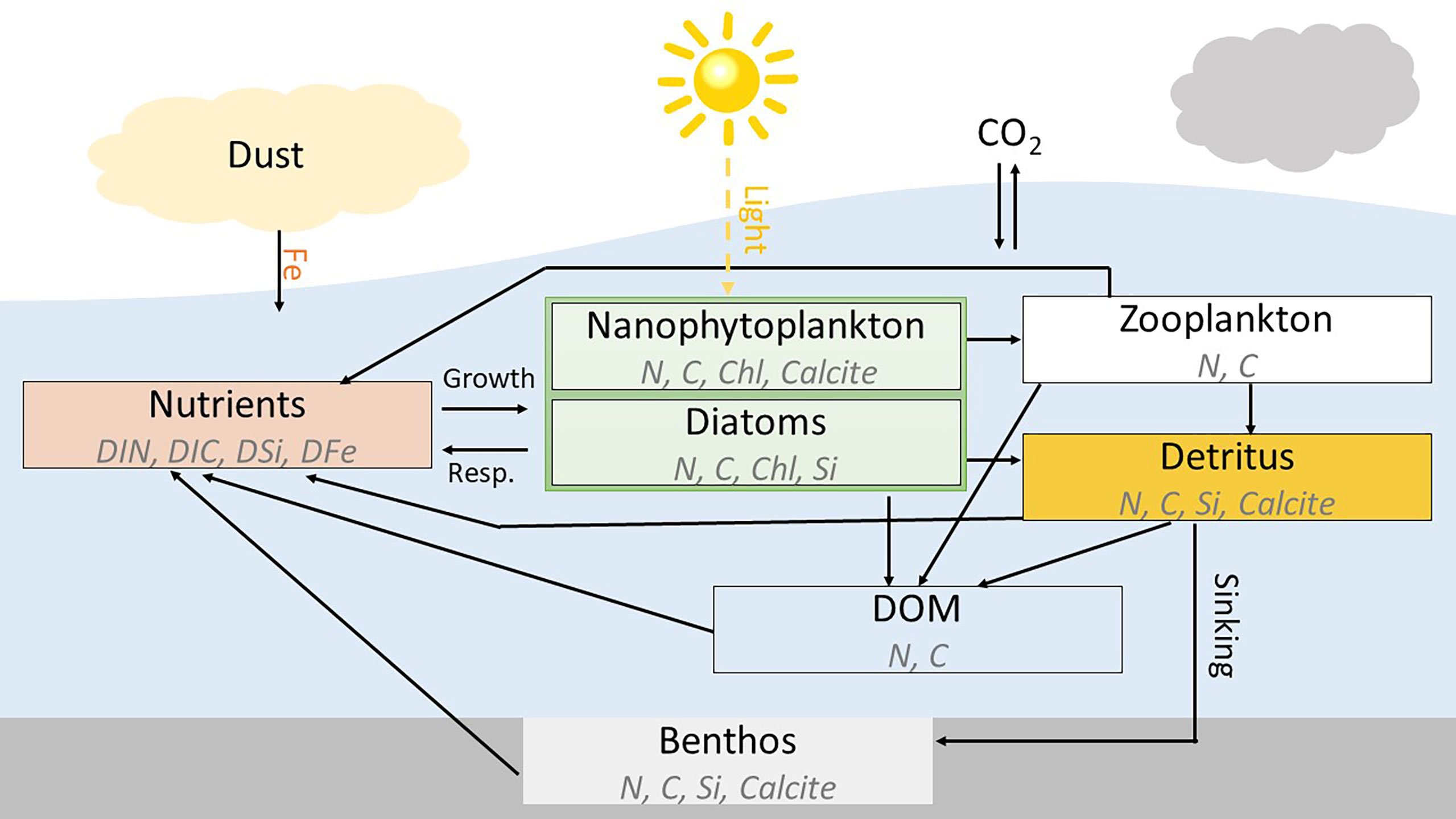
Figure 1 Schematic diagram of the ocean BGC model REcoM-2.

We used the Massachusetts Institute of Technology General Circulation Model (MITgcm, Marshall et al., 1997) to simulate ocean circulation and mixing. MITgcm solves the time-dependent, Boussinesq-approximated Navier–Stokes equations with or without hydrostatic approximation and conservation equations for salinity and energy. REcoM2 is coupled with MITgcm online at every time step, set up to 1 h (3,600 s). The total depth of the model setup is 1,188 m. The model has 30 vertical layers. The vertical grid spacing increases with depth from 10 m near the surface to 100 m near the bottom layer. As we are interested in ecosystem processes in the euphotic zone, and their coupling to vertical nutrient transports from the mesopelagic, we have limited our model setup to a bit more than the upper 1,000 m, well above the sea floor for both sites. Thus, the total depth of the model setup is independent of location and bathymetry.

The coupled MITgcm-REcoM2 model is configured in a 1-D vertical configuration at the geolocations of BATS (31°40′N, 64°10′W) located in the subtropical gyre of the North Atlantic (Sargasso Sea) and DYFAMED (43°25′N, 7°52′E) located in the Liguro-Provencal current of the Ligurian Sea at the northwestern Mediterranean Sea. Both stations have long-term time-series records with a wide variety of BGC variables. The choice of using two different stations in this study is to gain a better insight into the same BGC processes under different environmental conditions.

BATS and DYFAMED provide contrasting sampling schemes and environments. At BATS, the mesoscale eddies are a significant feature in the Sargasso Sea and impart an additional level of BGC variability (Sweeney et al., 2003). On the other hand, the BGC variability at DYFAMED is mainly induced by the seasonal succession of hydrological conditions (de Fommervault et al., 2015). DYFAMED has a shallower mixed layer compared with BATS in summer and fall (off-peak period) because it is highly saline (>38 psu) with a very shallow thermocline (Marty and Chiaverini, 2010). Another distinct feature of DYFAMED is that it receives significant atmospheric input from the deserts of North Africa and the industrialized countries bordering the Mediterranean Sea (Marty, 2002), which allows phytoplankton to grow at the surface even in the oligotrophic period. As a result of shallower mixed layer depth and large atmospheric nutrient deposition, DYFAMED has higher surface chl-a and lower vertically integrated net primary production (NPP) during the off-peak period compared with BATS. Notably, despite being close to the coast, DYFAMED is protected from lateral inputs by a coastal current, acting as a barrier to exchanges with the coastal zone.

We initialized the temperature, salinity, dissolved oxygen, nitrate, and silicate fields of the model at both stations with in situ bottle data obtained for BATS from its website (BATS Team, 2020) and for DYFAMED from Coppola et al. (2021). The total alkalinity and dissolved inorganic carbon fields at BATS were initialized with data from the mapped climatology of the GLobal Ocean Data Analysis Project (GLODAPv2, Lauvset et al., 2016). At DYFAMED, these fields were initialized from bottle data (Coppola, et al. 2021). The dissolved iron is initialized with data from the U.S. GEOTRACES North Atlantic Transect (GA-03, Boyle et al., 2015) at BATS and from the data reported in Guieu and Blain (2013) at DYFAMED. All other passive tracers were initialized with small uniform values. We use inter-annually varying atmospheric forcing—the Coordinated Ocean Research Experiments version 2 (COREv2, Large and Yeager, 2008) for BATS and ERA5 hourly data on single levels (Hersbach et al., 2020) for DYFAMED. Iron deposition was estimated from the monthly present-day simulation of Albani et al. (2014) at both stations.

To prevent long-term drifting and to avoid compensating for hydrographic errors caused by the 1-D setup, which ignores lateral advection, we apply a relaxation of temperature and salinity at every time step from the surface down to 400 m depth at BATS and from the surface down to 250 m at DYFAMED. The relaxation depth was determined as no clear seasonal temperature variability can be observed below this depth according to the long-term bottle data.

We additionally applied restoring sea surface salinity (SSS) to the monthly climatology with a timescale of 10 days at BATS and 2 days at DYFAMED. The monthly climatology of SSS was calculated from the in situ bottle data at both stations. At DYFAMED, whereas the vertical processes dominate in setting water properties, the lateral advection still plays a major role (Béthoux et al., 1998). However, the cyclonic circulation of the Ligurian Sea is not represented in the 1-D framework at this site. During the phase of intense and dry winds associated with surface buoyancy loss, the advection of homogeneous water columns becomes dominant and drives a doming of isopycnals that drift away from the 1-D model SSS from its climatology more frequently than BATS. This drifting of model SSS leads to a deeper mixed layer at DYFAMED in the winter. This required us to restore SSS more frequently at DYFAMED than BATS.

2.2 Data assimilation

2.2.1 Observational data

We assimilate two sets of observations: i) satellite chl-a concentration and ii) in situ vertically integrated NPP.

We obtained the satellite chl-a concentration data from the ESA (European Space Agency) Ocean Color Climate Change Initiative (OC-CCI, Sathyendranath et al., 2019) time-series data product. It is a daily merged product of MODIS-Aqua, MERIS, SeaWiFS, and VIIRS on a sinusoidal grid at 4-km resolution. We downloaded the 5-day average dataset via FTP from the OC-CCI website (European Space Agency, 2021). We take an area of a 1° square at each site and average all available values in the area as the representative data value for the station.

The chl-a concentrations provided in the OC-CCI dataset are not bias-corrected. However, the dataset provides per pixel biases and root mean square deviation. We calculate the unbiased chl-a concentration and its variance based on Appendix A of Ciavatta et al. (2016). The variances were used as observation errors in the DA. Figure 2A shows the average chl-a concentration (green dots) in 5-day intervals and its standard deviation as error bars at BATS. From the error bars, large uncertainty is evident in the data. As the chl-a concentration is lognormally distributed (Campbell, 1995), we used logarithmically transformed (log‐transformed) concentrations in the DA implementation.

FIGURE 2

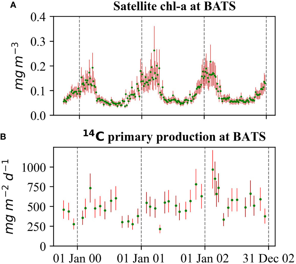
Figure 2 Observational data during the study period at BATS. (A) OC-CCI satellite chl-a concentration. The green dots depict data values, and the red lines depict standard deviations. (B) Vertically integrated NPP (green) and assumed errors (red).

We obtained the ¹⁴C primary production data for BATS from the BATS website (BATS Team, 2020) and for DYFAMED from Coppola et al. (2021). The methods for the sample collection and the calculation of ¹⁴C primary production are described in the US Joint Global Ocean Flux Study (JGOFS) protocol (JGOFS, 1997; Laws et al., 2002) for BATS and Marty et al. (2008) for DYFAMED. We calculated the water column integrated NPP in mgCm^-2d^-1from the measurements at individual depths by trapezoidal integration, assuming that the rate from the surface to the nearest measure is constant and the rate after 200 m is zero (see JGOFS, 1997). Figure 2B shows the integrated NPP at BATS from October 1999 to December 2002. For all DA runs, we assume a Gaussian error distribution with a relative error of 0.25 for NPP at both stations.

2.2.2 DA method

The DA was performed using the Parallel Data Assimilation Framework (PDAF; Nerger and Hiller, 2013)¹1

http://pdaf.awi.de/

— a free and open-source software designed to implement ensemble DA with existing numerical models. PDAF provides fully implemented and optimized DA algorithms, particularly ensemble-based Kalman filters. We applied the ensemble‐based Error‐Subspace Transform Kalman Filter (ESTKF; Nerger et al., 2012) in this study. The ESTKF is an ensemble square root filter that computes the weights for the ensemble transformation directly in the error-subspace represented by the ensemble.

We used a 108-member ensemble. To make the BGC processes slightly different in each ensemble member and generate varying model states (ensemble members), we randomly perturbed 10 parameters. The parameters are chosen following earlier studies (e.g., Hu et al., 2012; Doron et al., 2013; Ciavatta et al., 2016; Pradhan et al., 2019; Pradhan et al., 2020) and model descriptions (e.g., Hauck et al., 2013; Schourup-Kristensen et al., 2014) that they control the key BGC processes of the model and that their values are poorly constrained. As we assimilated chl-a concentration and NPP data, we focused on the parameters related to phytoplankton production and to those that directly influence phytoplankton mortality. Four of the selected parameters are related to phytoplankton sources, whereas the remaining six are related to the phytoplankton sinks.

A brief description of the 10 selected parameters is provided below. A list of all REcoM2 parameters can be found in the Supplementary Document.

2.2.2.1 Maximum photosynthesis rate of nanophytoplanktons (${\mu }_{Nano}^{max}$) and diatoms (${\mu }_{Dia}^{max}$)

Phytoplankton takes up nutrients from the inorganic nutrient pool and energy from the sunlight to produce biomass to grow. The process is known as photosynthesis. REcoM2 calculates the C-specific photosynthesis (P) based on the maximum photosynthesis rate P^max that has an intrinsic maximum growth rate of μ^max (time⁻¹) and is limited (0< f_lim<1 ) by either physical conditions (e.g., temperature and turbulence) or resources such as light, nutrients, and dissolved inorganic carbon.

$$P^{max}= {\mu }^{max}. f_{lim}$$

P is calculated for both nanophytoplanktons (P_Nano) and diatoms (P_Dia) based on Geider et al. (1998) using maximum photosynthesis rate for nanophytoplankton (${\mu }_{Nano}^{max}$) and for diatoms (${\mu }_{Dia}^{max}$). It differs between nanophytoplankton and diatoms in the nutrient limitation; nanophytoplankton is limited by iron and nitrogen, whereas diatoms are additionally limited by silicon, hence constraining different values for the two groups.

$$P^{max}= {\mu }^{max}.f_T.\left(f_{lim}^{Fe},f_{lim}^{N:C_{min}}\right)$$

where f_T is an Arrhenius function of temperature dependency. f^Fe , $f_{lim}^{N:C_{min}}$, and $f_{lim}^{N:C_{min}}$ are growth-limitation by iron, nitrogen, and silicon and are calculated using the Liebig law of the minimum, in which the most limiting nutrient limits production (O'Neill et al., 1989).

2.2.2.2 Initial slope of the photosynthesis-irradiation (P-I) curve of nanophytoplankton (α_Nano) and diatoms (α_Dia)

P depends on how much photosynthetically available radiation (PAR) the cell can harvest. This is controlled by the initial slope of the P-I curve (α), which represents the photosynthetic efficiency under light levels close to zero and is obtained by multiplication of the light-harvesting efficiency per chlorophyll with the intracellular chlorophyll to carbon ratio (q^Chl:C).α is used to model P as a saturating function of PAR.

$$P=P^{max} \left(1-exp \left(\frac{- \alpha . q^{Chl:C}.PAR}{P^{max}}\right) \right)$$

The C-specific photosynthesis rate, P, is calculated for both nanophytoplankton (P_Nano) and diatoms (P_Dia) with α_Nano and α_Dia , respectively.

2.2.2.3 Chlorophyll degradation rate of nanophytoplanktons ($d_{Nano}^{chl}$) and diatoms ($d_{dia}^{chl}$)

Chlorophyll concentrations are used as a proxy for living phytoplankton biomass. Photoinduced and microbial processes can degrade chlorophyll before the phytoplankton dies or is eaten by the zooplankton. In REcoM2, chlorophyll is degraded with a fixed rate d^chl that contributes to the overall chlorophyll loss and, in turn, phytoplanktonic carbon loss. As phytoplanktonic carbon loss is calculated for both nanoplankton and diatom, REcoM2 uses two chlorophyll degradation rate parameters $d_{Nano}^{chl}$ and $d_{dia}^{chl}$ for nanoplankton and diatom, respectively.

2.2.2.4 Maximum grazing rate (ξ) and grazing efficiency (γ)

Zooplanktons consume phytoplankton in a process known as grazing. The grazing function describes a rectangular hyperbolic relationship between phytoplankton nitrogen (N) abundance, with a sigmoidal dependency of nutritional intake to resource density with an N-specific maximum grazing rate (ξ). It depends on temperature following the same relationship as for phytoplankton growth (f_T). The grazing G on nanophytoplankton and diatoms is defined as follows:

$$G= \xi .\frac{{\left(N_{Nano}+N_{Dia}^{\text{'}}\right)}^2}{{\phi }_1+\left(N_{Dia}+N_{Dia}^{\text{'}}\right)} . f_T.N_{het}$$

$N_{Dia}^{\text{'}}$ encompasses a preference term for grazing on diatoms, relative to that on nanophytoplankton:

$$N_{Dia}^{\text{'}}= \tau .\frac{N_{Dia}^2}{{\phi }_2+ N_{Dia}^2} . N_{Dia}$$

Here, τ is the maximum diatom preference and is smaller than 1, which implies that zooplankton grazes preferably on nanophytoplankton; the effective grazing preference is allowed to vary with diatom biomass, with φ₂ being the half-saturation parameters for grazing preference of diatoms. φ₂ = 0 implies a constant preference.

The phytoplankton biomass that enters the zooplankton may be incorporated into new biomass, voided through defecation to Pellets assuming a fixed grazing efficiency (γ) that determines how much of the grazed phytoplankton is built into heterotrophic biomass.

2.2.2.5 Specific aggregation rate of phytoplankton ( ∅_Phy) and detritus ( ∅_Det)

A non-physiological mortality term denoted as aggregation loss describes a part from the grazing loss of phytoplankton to sinking detritus. The removal of material from oceanic surface waters and its subsequent transport to the ocean interior is driven by the formation and sinking of particles. However, only larger particles with high settling rates significantly contribute to the vertical flux reaching the sea floor (McCave, 1984). The collection of smaller particles into larger ones is called aggregation. The aggregation rate g is assumed to be proportional to the abundance of phytoplankton and detritus:

$$g= {\varnothing }_{Phy}.N_{Nano}+ {\varnothing }_{Phy}.N_{Dia}+ {\varnothing }_{Det}.N_{Det}$$

where the phytoplankton-specific aggregation rate (∅_Phy) and detritus-specific aggregation rate (∅_Det) reflect the roles of phytoplankton and detritus in the aggregation process. Phytoplankton-specific aggregation rate, ∅_Phy , is assumed to be the same for nanoplanktons and diatoms.

We keep the reference values, hereafter referred to as the default values, of the parameters as used in Hauck et al. (2013). We perturbed the parameters assuming a lognormal distribution with a relative variance of 0.25 for all the selected parameters. Hence, each ensemble member was started from the same initial condition but with different values for the perturbed parameters. The DA process was initialized from the ensemble of model states at the end of the spin-up period (see 2.2.3).

We estimated eight BGC model state variables, total chl-a, and vertically integrated NPP using the ESTKF in all DA simulations. The eight model state variables are as follows:

1. Nanophytoplankton content of carbon

2. Diatom content of carbon

3. Nanophytoplankton content of nitrogen

4. Diatom content of nitrogen

5. Nanophytoplankton calcium carbonate

6. Biogenic silica for diatoms

7. Nanophytoplankton chl-a

8. Diatom chl-a

Note that total chl-a and vertically integrated NPP are diagnostic model variables. For these two diagnostic variables, the observation operator selects the corresponding values from the state vector. The eight model state variables are updated through the ensemble‐estimated cross covariances to total chl-a and vertically integrated NPP when observations are available. The total chl-a and the vertically integrated NPP estimated by the DA process are not distributed to the model but stored as diagnostic variables.

One issue of parameter estimation through DA is that, in the analysis step, the value of parameters in each ensemble member changes toward the optimal values. As a result, the ensemble spread decreases, and the parameter ensemble may collapse before an optimal parameter value is found. To avoid this, we inflated the variance of the parameter ensemble in every assimilation cycle by 2.56%.

2.2.3 DA experiment

DA experiments were performed from October 1999 to December 2002 for BATS and from October 1997 to December 2000 for DYFAMED. The difference in the chosen period was caused by the availability of the in situ bottle NPP data. The model was first run with 108 ensemble members using the perturbed parameters from January 1990 as a spin-up for both stations. We conducted three types of DA experiments.

● EXP_{State_DP} — State estimation with the default parameters: We performed state estimation experiments with the default parameters as the reference simulations.

● EXP_{Joint_DP} — Joint state-parameter estimation: In these experiments, we augmented the state vector by the 10 selected BGC parameters and updated them in each assimilation cycle together with the state variables. Therefore, the selected parameters vary over time in this experiment.

● EXP_{State_EP}— State estimation with estimated parameters: To assess the effect of the estimated parameters on model prediction, we performed state estimation experiments (DA runs for model state) with the estimated parameters.

For each type of experiment, we implemented four simulations: i) Free-run (ensemble run without DA), ii) satellite chl-a only assimilation, iii) vertically integrated NPP only assimilation, and iv) combined assimilation of satellite chl-a and vertically integrated NPP. The free-run simulation of EXP_{Joint_DP} is identical to the free-run simulation of EXP_{State_DP}. Therefore, we did not repeat the free-run simulation in the EXP_{Joint_DP}.

3 Results

In this section, we first present the results of the joint state‐parameter estimation from the EXP_{Joint_DP} (Section 3.1), particularly the estimation of 10 model parameters. Then, we assess the performance of the estimated parameters (EXP_{State_EP}) compared with the reference simulations (EXP_{State_DP}), state estimation with the default parameters) and the prediction capabilities of DA in general for both stations (Section 3.2).

3.1 Joint state‐parameter estimation (EXP_{Joint_DP})

The ensemble evaluation of surface chl-a concentration and vertically integrated NPP shows that the free-run with default parameters (EXP_{Joint_DP}) performs poorly at both stations (Figure 3). At BATS, the free-run overestimates the surface chl-a concentration compared to satellite data (Figure 3A) and underestimates the NPP compared to bottle data (Figure 3B). The free-run performs better at DYFAMED than at BATS for surface chl-a concentration. At DYFAMED, the model produces realistic surface chl-a concentrations during the bloom period but overestimates them during the oligotrophic periods (Figure 3C). NPP is overestimated at DYFAMED for both free-run and combined assimilation of EXP_{Joint_DP} (Figure 3D). The simulation with combined assimilation of satellite chl-a and vertically integrated NPP of EXP_{Joint_DP} performs better because the filter brought the model state close to the observations during the first bloom period for both stations.

FIGURE 3

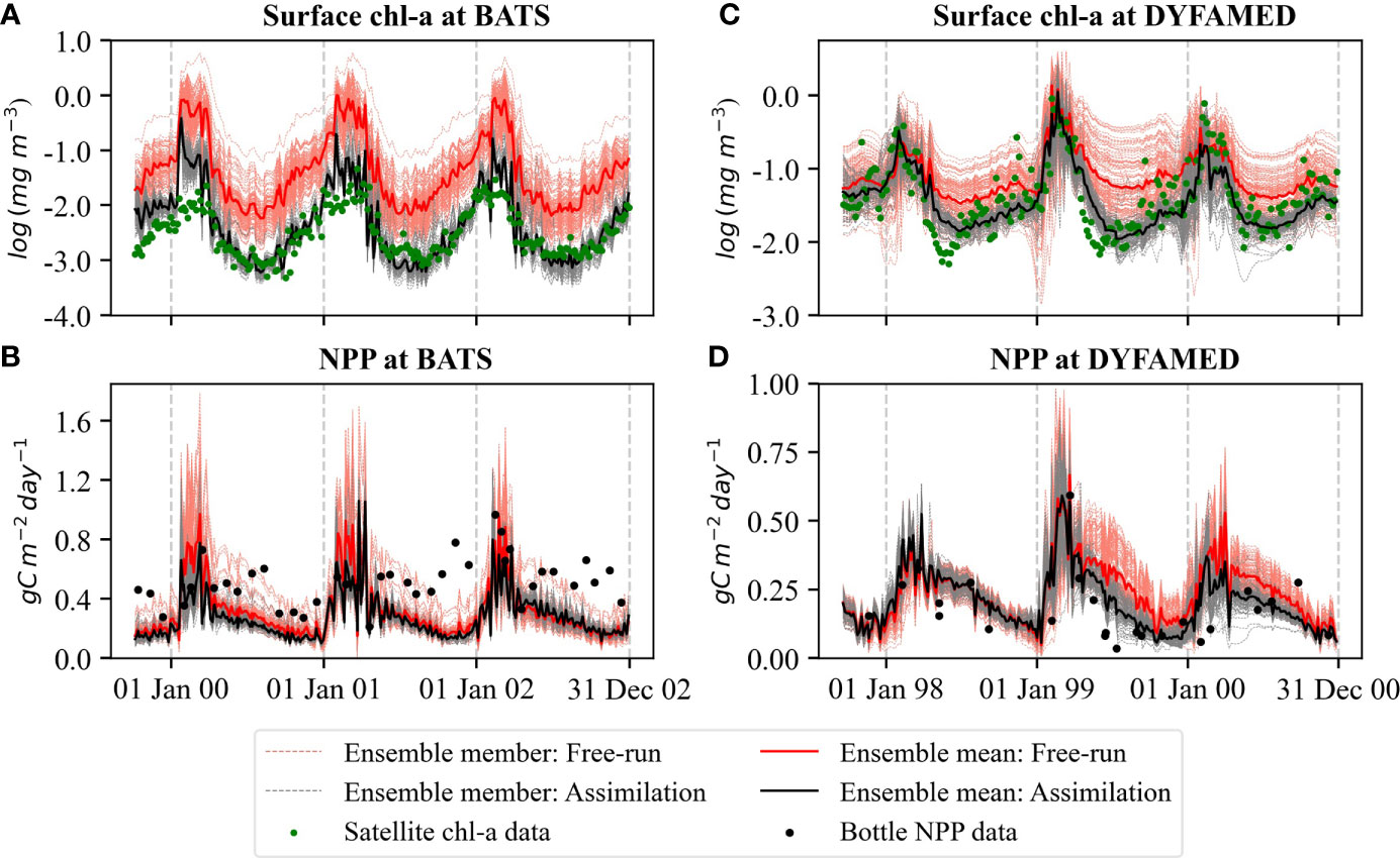
Figure 3 The ensemble evaluation of log-transformed surface chl-a concentration at (A) BATS and (C) DYFAMED, and NPP at (B) BATS and (D) DYFAMED for joint state-parameter estimation (EXP_{Joint_DP}). The red dashed lines show ensemble members for the free-run, and the solid red line shows their mean. Gray dashed lines are ensemble members of the simulation with combined assimilation of satellite surface chl-a and in situ NPP data, and the solid black line is their mean. The green dots represent observations (satellite data for surface chl-a and bottle data for NPP).

NPP shows larger discrepancies at BATS. The filter even pushed the NPP simulation away from the observations at the station to compensate for the correction in the surface chl-a concentration. In the DA process, satellite chl-a data had a stronger influence than the in situ ¹⁴C primary production data on the overall change of the states.

3.1.1 Evaluation of parameter estimates

We estimate values of the same 10 parameters (Section 2.2.2) that were perturbed to generate the ensembles at both stations. The objective was to get an optimized set of parameters to improve the model prediction, from which we can gain insight into the interaction between phytoplankton growth and decay. The minimization of the model-data misfit in the assimilation run compared with that in the free-run presented above is mostly due to the simultaneous update of the selected parameters. The value of parameters obtained at the final DA cycle (time step) is the estimated parameter value. Table 1 shows the default values and estimated values at the end of the experiment of the 10 selected parameters for both stations.

TABLE 1

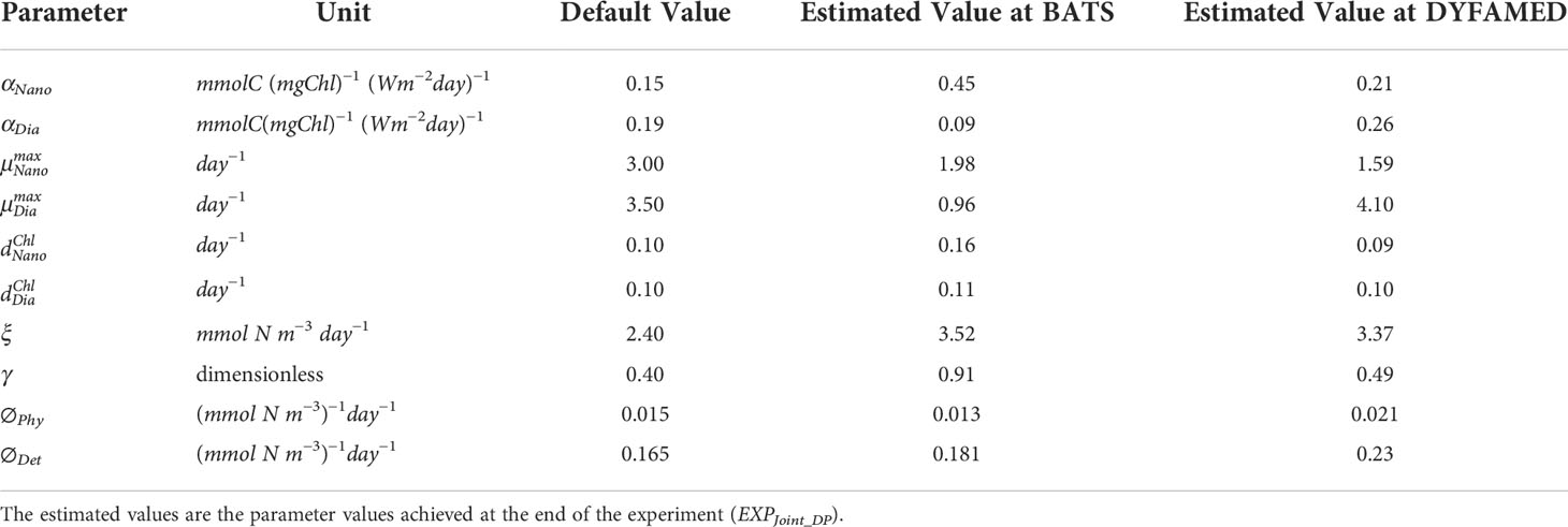
Table 1 The 10 BGC parameters that are estimated in this study: the default and the estimated values.

The initial slope of the photosynthesis-irradiance (P-I) curve of nanoplankton (α_Nano) and diatom (α_Dia), the maximum photosynthesis rate of nanoplankton (${\mu }_{Nano}^{max}$), and the maximum grazing rate (ξ) were changed the most at both stations. The maximum photosynthesis rate of diatoms (${\mu }_{Dia}^{max}$), nanoplankton chlorophyll degradation rate ($d_{Nano}^{Chl}$), and grazing efficiency (γ) were changed significantly at BATS but not much at DYFAMED. The two aggregation parameters, the phytoplankton-specific aggregation rate (∅_Phy), and the detritus-specific aggregation rate (∅_Det) were changed significantly only at DYFAMED. Significant change refers to more than one-third (36%) of change after the final DA time step.

The ensemble evaluations of all 10 parameters for satellite chl-a only assimilation and combined assimilation of satellite chl-a and vertically integrated NPP resulting from the EXP_{Joint_DP} for both stations are presented in the Supplementary Document. Here, we focus on the parameters that changed significantly at one or both stations when assimilating both datasets in the experiment EXP_{Joint_DP} and examine their temporal evolution and variability at the two stations.

The evolution of the assimilated values of α_Nano and ${\mu }_{Nano}^{max}$ for both stations is shown in Figure 4. At BATS, α_Nano reached a final value of 0.45 and had much larger updates (increased more than 200% than its initial value) than at DYFAMED where the parameter increased 50% from the initial value (Figures 4A, C, Table 1). The large change at BATS is related to the large bias of surface chl-a compared to observations (see Figure 3). At DYFAMED, on the other hand, the model without DA represented the surface chl-a much better (see Figure 3). The value of α_Nano at DYFAMED was increased from the default value of 0.15 by around 50% in the first year and stabilized after that for the rest of the assimilation period with a final value of 0.21 (Figures 4B, D, Table 1). This change could relate to the overestimation of surface chl-a during the off-peak period at this site.

FIGURE 4

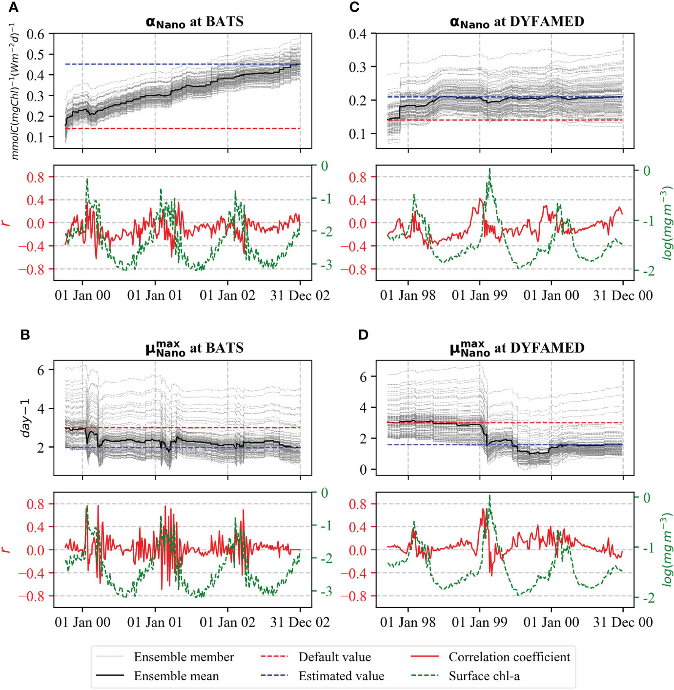
Figure 4 Evaluation of α_Nano for (A) BATS and (C) DYFAMED and ${\mu }_{Nano}^{max}$ for (B) BATS and (D) DYFAMED for combined assimilation of satellite surface chl-a and in situ NPP simulations of EXP_{Joint_DP}. Top panels show the ensemble evaluation (gray dashed line) and the associated ensemble means (black solid line). The default and estimated values are shown as dashed lines (red for default and blue for estimated). The bottom panels show the correlation of parameter value with the observed surface chl-a concentration at each assimilation cycle.

At both stations, the reduction of surface chl-a concentration led to a decrease in ${\mu }_{Nano}^{max}$ that is partly compensated by an increase in α_Nano . The value of ${\mu }_{Nano}^{max}$ decreased around one-third after the first spring bloom at BATS (Figure 4B). Approximately, the same value is reached after the later blooms, whereas it is slightly higher during the off-peak periods. At DYFAMED, updates to ${\mu }_{Nano}^{max}$ occurred only during the second bloom period with a decrease of around 45% (Figure 4D).

The change in α_Nano and ${\mu }_{Nano}^{max}$ was induced by the correlation between the observations and the model resulting from the ensemble. At both stations, α_Nano is negatively correlated with surface chl-a concentration during off-peak periods, whereas the correlation coefficient becomes positive at the beginning of the bloom periods (Figures 4A, C, bottom panels). For ${\mu }_{Nano}^{max}$, the correlation is also positive around the beginning of blooms. However, it does not show extended periods of negative values (Figures 4B, D, bottom panels). These correlations also denote that a varying dependence between the photosynthesis parameters and the seasonal ecosystem variability exists. Lower values of correlation coefficients between surface chl-a concentration and α_Nano during the bloom period indicate that this parameter is difficult to constrain with surface chl-a and uncertainty increases during a bloom period.

The loss parameter $d_{Nano}^{Chl}$ increased by 60% at BATS and decreased by 10% at DYFAMED from its initial value at the end of the experiment with a final value of 0.16 and 0.09 day⁻¹, respectively (Figure 5). At BATS, $d_{Nano}^{Chl}$ first increased by around 80% after the first bloom period, further increased slightly during the second bloom period, but then decreased slightly until the third bloom period (Figure 5A). This suggests high uncertainty of $d_{Nano}^{Chl}$ at BATS. Similarly, at DYFAMED, the parameter increased first and then decreased after the second bloom period. This indicates that parameter values can have large inter-annual variation (Figure 5B).

FIGURE 5

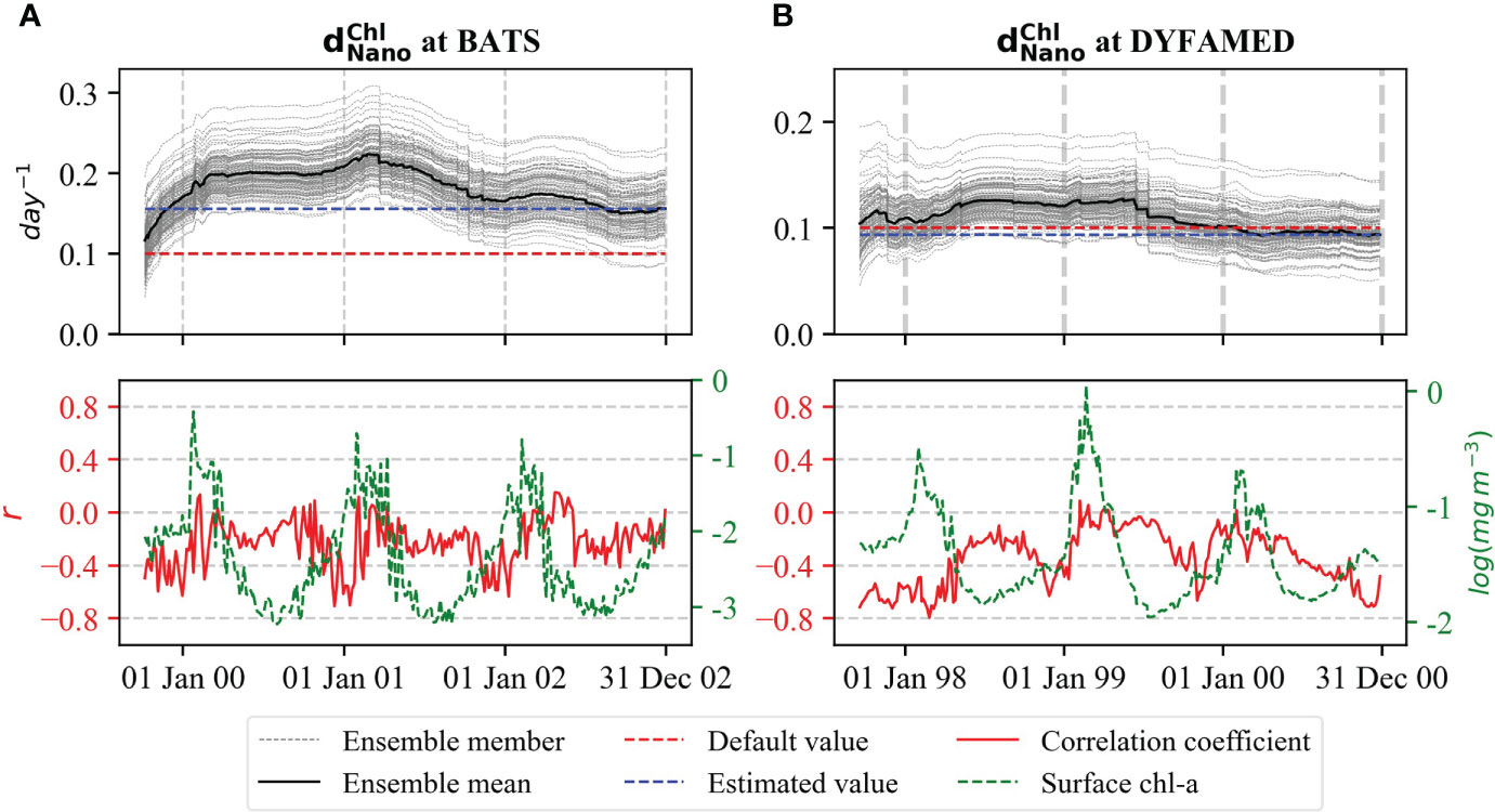
Figure 5 Evaluation of $d_{Nano}^{Chl}$ rate for (A) BATS and (B) DYFAMED analogous to - Figure 4.

For both stations, the correlation of $d_{Nano}^{Chl}$ with surface chl-a is significant during the beginning of the bloom and becomes weaker later in the bloom period. One possible explanation for this weak correlation is that, during the bloom period, grazing becomes prominent for loss of chl-a, and thus, the grazing parameters compensate $d_{Nano}^{Chl}$. At BATS, the high variability of the correlation coefficient indicates high uncertainty of the parameter at the station.

For the grazing parameters ξ and γ , Figure 6 shows the ensemble members and their means. The value of ξ is increased from its default value by around 50% in the first spring bloom at BATS (Figure 6A). In contrast, it remained nearly unchanged at DYFAMED during the first year but increased by around 40% in the second spring bloom (Figure 6B). This behavior could be related to the higher bias of the free-run simulations (overestimation of surface chl-a) during the second year at DYFAMED. In the first year, the bias was compensated by other parameters, e.g., α_Nano and $d_{Nano}^{Chl}$.

FIGURE 6

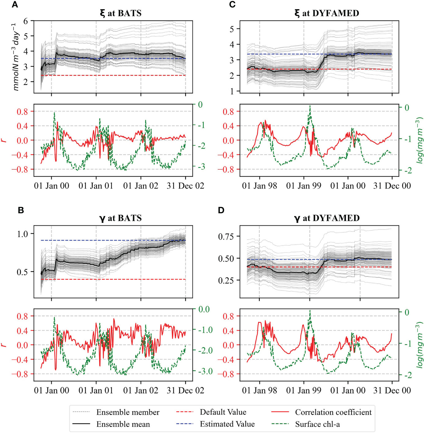
Figure 6 Evaluation of ξ for (A) BATS and (C) DYFAMED, and γ for (B) BATS and (D) DYFAMED analogous to Figure 4.

Whereas at BATS, γ increased by around 125%, at DYFAMED, the increase was smaller, which is around 20% (Figures 6C, D). γ appears to show a continuously increasing trend at BATS from the beginning of the second bloom period.

Both grazing parameters showed a similar pattern of correlation with surface chl-a. At BATS, we see a positive correlation to the surface chl-a, mainly during the off-peak periods (Figure 6C). On the contrary, the correlation is mainly positive during the bloom periods and negative at the other times of the year at DYFAMED (Figure 6D).

The aggregation parameter ∅_Phy decreased slightly at BATS (Figure 7A) but increased at DYFAMED between the first and second spring bloom with a final value of 0.021, which is about 40% larger than the default value (Figure 7B). This change is connected to a negative correlation between the parameter and chl-a at the station. At DYFAMED, ∅_Phy is negatively correlated after the first bloom termination to the next initialization when its values change. From the second bloom, the parameter reaches a stable value and shows only a weak correlation. On the other hand, ∅_Phy is not well correlated with surface chl-a at BATS, which explains minor changes in the parameter in the station (Figure 7A). The other aggregation parameter ∅_Det also exhibits a similar pattern as ∅_Phy (not shown).

FIGURE 7

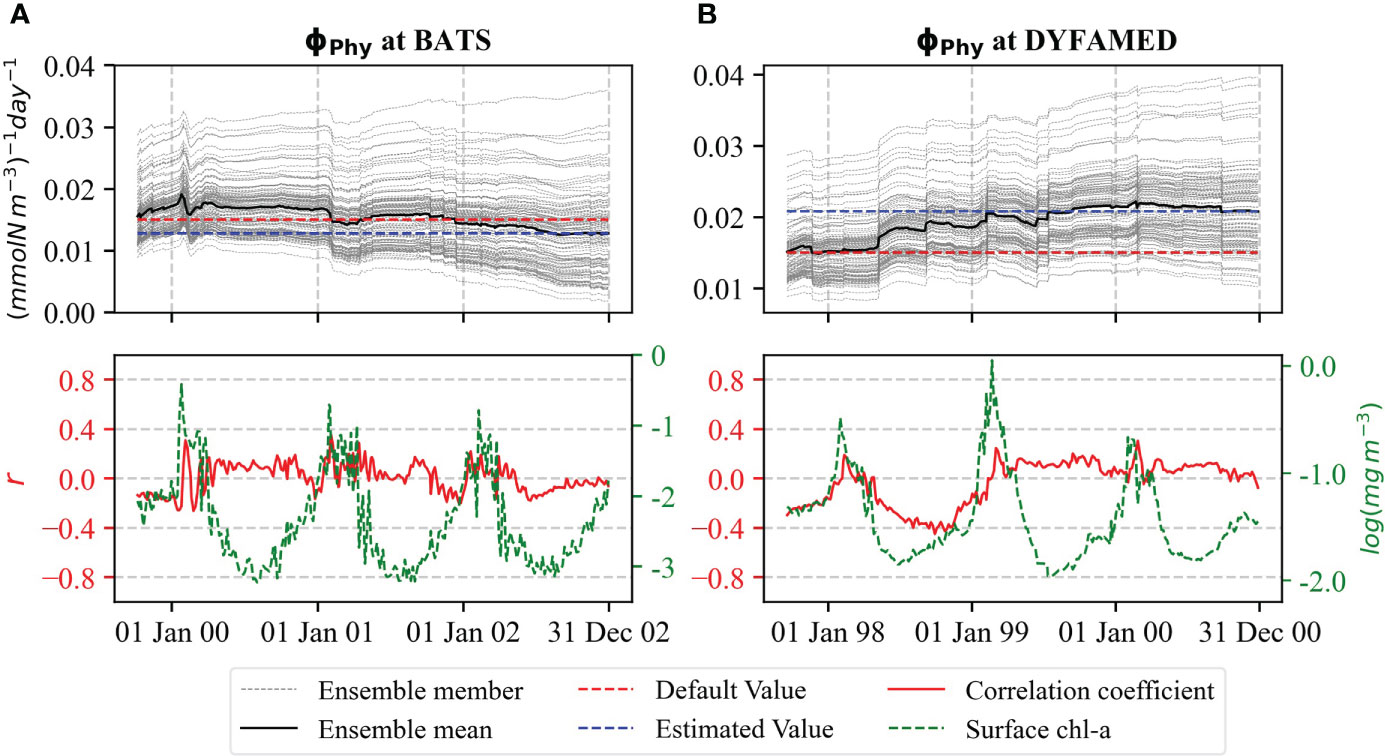
Figure 7 Evaluation of ∅_Phy for (A) BATS and (B) DYFAMED analogous to Figure 4.

3.1.2 Correlation among the parameters

To assess how strongly different parameters are correlated, we computed the Pearson correlation coefficients between each possible pair of parameters over time for both stations. The correlations are shown in Figure 8. Using T-test to determine statistical significance, there are five parameter pairs at BATS (Figure 8A) and three pairs at DYFAMED (Figure 8B) for which it is possible to reject the null hypothesis of no correlation at the p = 0.01 probability level. The explanation of the computed relationships is as follows:

● α_Nano versus ${\mu }_{Nano}^{max}$: Increases in α_Nano mean that less chl-a is required to achieve the same primary production, whereas increases in ${\mu }_{Nano}^{max}$ result in higher chl-a production. Therefore, balance among chl-a concentration and NPP accounts for the negative relationship between these two photosynthesis parameters. The correlation at both sites becomes significant after the first year of parameter estimation, pointing out that the optimal values of these two parameters depend on each other.

● ξ versus γ : Increases in both grazing parameters ξ and γ reduce the yield of chl-a concentration, accounting for the positive relationship. The correlations decreased over time and became insignificant when the value of the parameters got optimal. Constraining these two parameters individually may produce unrealistic values.

● α_Nano versus $d_{Nano}^{Chl}$: Decreases in α_Nano increase chl-a concentration for the same primary production, whereas increases in $d_{Nano}^{Chl}$ compensate for this by decrementing chl-a concentration before decease of the phytoplankton, accounting for the negative relationship.

● $d_{Nano}^{Chl}$ versus ξ : Increase in the chlorophyll degradation rate reduces the abundance of phytoplankton. Hence, the zooplankton can graze less, which accounts for the negative relationship.

● $d_{Nano}^{Chl}$ versus γ : Similar to the previous point, a higher chlorophyll degradation rate means less phytoplankton abundance for grazing. $d_{Nano}^{Chl}$ is strongly correlated with both ξ and γ at BATS only because of the large overestimation of the surface chl-a concentration at the station. This large overestimation is not present at DYFAMED.

● $d_{Nano}^{Chl}$ versus ∅_Phy : Increases in chlorophyll degradation result in decreased aggregations of senescent cells. Aggregation is a significant pathway by which nanoplankton contributes to export production in low biomass environments (Jackson et al., 2005). Therefore, it accounts for negative correlations.

FIGURE 8

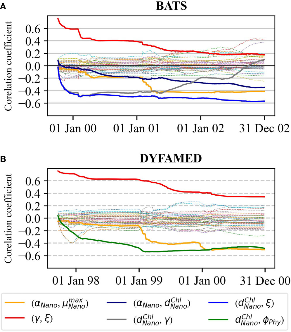
Figure 8 The Pearson correlation coefficients between each pair of the 10 biogeochemical parameters at (A) BATS and (B) DYFAMED. The solid lines denote significantly correlated pairs.

3.2 Model performance with estimated parameters

To evaluate the effect of the parameter estimation, we performed state estimation experiments (with perturbed parameters but no parameter estimation) using the default parameter values (EXP_{State_DP}) and the estimated parameter values (EXP_{State_EP}).

3.2.1 Surface chl-a and NPP

The log-transformed surface chl-a and its uncertainty estimate for both stations using default and estimated parameters over the study period are presented in Figures 9A, C. Root mean square errors (RMSEs) of simulated log-transformed surface chl-a against satellite (assimilated) and bottle (independent) data are summarized in Table 2. As seen in both Figures 9A, C, the estimated parameters improve the model predictions of surface chl-a concentration substantially at both sites. The RMSE of surface chl-a concentration simulations was reduced by about 66.67% against satellite data and about 44.78% against bottle data. At DYFAMED, RMSE for log-transformed surface chl-a concentration was reduced by 28.58% and 11.11% against satellite and in situ bottle data, respectively.

FIGURE 9

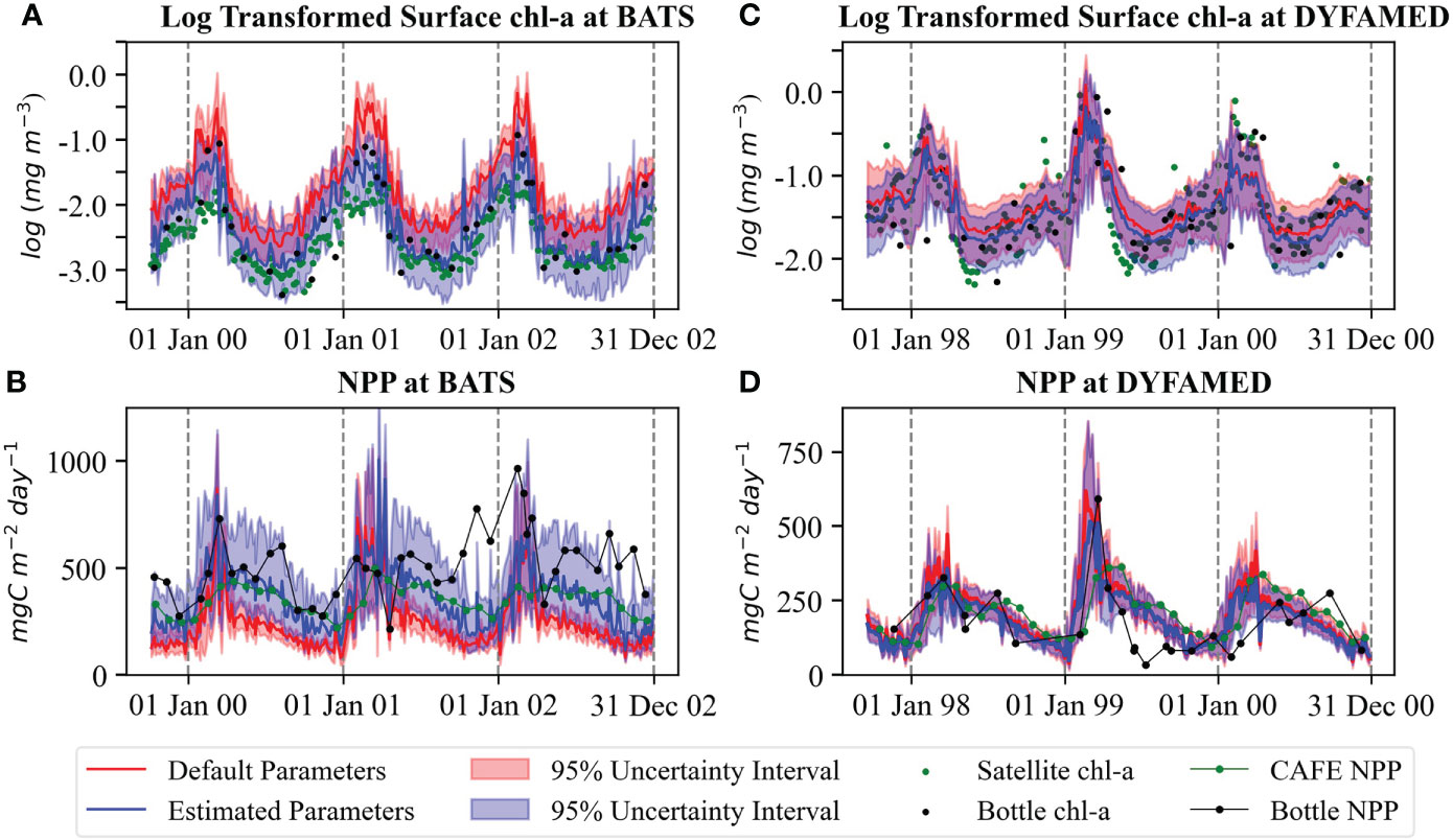
Figure 9 Comparison of log-transformed surface chl-a concentration of combined assimilation of satellite chl-a and in situ NPP simulations with default (EXP_{State_DP}) and estimated parameters (EXP_{State_EP}) at (A) BATS and (B) DYFAMED and of NPP simulations with default and estimated parameters at (C) BATS and (D) DYFAMED. The red line shows the ensemble mean with default parameters and the blue line is for estimated parameters. The green dots show satellite data, and the black dots are bottle data.

TABLE 2

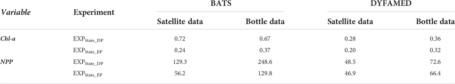
Table 2 RMSE of log-transformed surface chl-a concentration from combined assimilation of satellite chl-a and in situ NPP data of EXP_{State_EP} against satellite and bottle data at both stations.

The improvements are larger at BATS with a strong reduction of RMSE for log-transformed surface chl-a concentration. This large improvement is because the default parameters perform poorly at BATS. Most of the concentrations from satellite and bottle data fall below the ensemble from the simulation with default parameters at the station. However, they fall inside the ensemble range when the estimated parameters are used (Figure 9A). At DYFAMED, some observations fall outside of the ensemble for default parameters and remain outside of the ensemble for estimated parameters (Figure 9C). At DYFAMED, satellite data show brief blooms during autumn, which the model does not reproduce. A possible explanation can be that the model does not represent destratification correctly as the 1-D framework does not capture cyclonic circulation.

The predictions of NPP for default (EXP_{State_DP}) and estimated parameters (EXP_{State_EP}) and their uncertainty estimates are shown in Figures 9B, D. We compare NPP simulations with in situ bottle data (assimilated observation) and monthly satellite-derived data (independent observation) obtained from the Ocean Productivity website at the Oregon State University (Ocean Productivity, 2021). The satellite-derived data are NPP computed using the Carbon, Absorption, and Fluorescence Euphotic-resolving (CAFE) model (Silsbe et al., 2016) based on SeaWiFS satellite data. RMSEs of the ensemble mean NPP of combined satellite chl-a and in situ NPP assimilation of both EXP_{State_DP} and EXP_{State_EP} against in situ bottle and satellite-derived data are presented in Table 2. As can be seen, the estimated parameters largely improve the NPP prediction at BATS and little improvement at DYFAMED. Despite the improvement, there are still large discrepancies at BATS. The RMSE of NPP simulation was reduced by 56.5% against satellite data and 47.78% against in situ bottle data at BATS and by 3.30% and 8.54% against satellite-derived and bottle data, respectively.

At BATS, model simulations agree reasonably with satellite NPP estimations but show large discrepancies with the bottle data. The concentrations in bottle data are much higher, particularly during oligotrophic periods. Notably, the bottle data at BATS show no apparent seasonality. Because of this behavior, we suspect large uncertainty in the ¹⁴C NPP measurements. At DYFAMED, the improvements are smaller compared with BATS.

3.2.2 Phytoplankton phenology indices

To further assess the influence of the estimated parameters, we examine five phytoplankton bloom phenology indices, namely, i) initiation, ii) peak time, iii) termination time, iv) duration, and v) peak value. At both stations, the initiation generally occurs in December/January (Figures 10A, F), bloom peaks mostly 4–6 weeks later (Figures 10B, G), and the termination is in March/April (Figures 10C, H). Differences in the timing of these phenological events between the simulations with default (EXP_{State_DP}) and estimated parameters (EXP_{State_EP}) are relatively small, with the observed timing of these indices falling within the ensemble range.

FIGURE 10

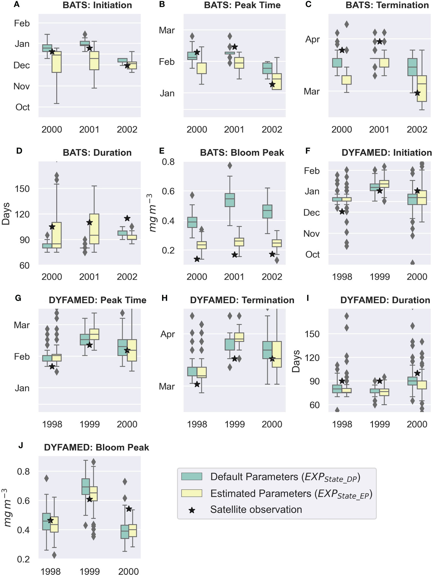
Figure 10 Phytoplankton phenology metrics (A–E) bloom initiation, peak time, termination, duration, and peak value at BATS and (F–J) DYFAMED. The black stars are calculated from satellite data; the boxes show the quartiles of the ensemble of the combined chl-a and NPP assimilation, whereas the whiskers extend to show the rest of the ensemble members except for points determined to be “outliers” using the inter-quartile ranges.

At BATS, the range for these phenological timings is broader, indicating a large uncertainty of these matrices on the selected BGC parameters, at least the parameters that we selected in this study. At both stations, the model-simulated bloom duration is shorter than the satellite observation. At BATS, the bloom duration with estimated parameter values falls within the ensemble range for the first and second years (Figure 10D). However, it gets even shorter in the third year. At DYFAMED, bloom durations with estimated parameter values did not change much compared with default parameter values (Figure 10I). The blooms occur earlier at BATS for EXP_{State_EP}, with its peak concentrations being strongly reduced compared with EXP_{State_DP} and coming closer to the observations (Figure 10E). Estimated parameter values had less influence on the peak concentration at DYFAMED (Figure 10J). At DYFAMED, the bloom peaks in both model and observation have higher chl-a concentration than at BATS. However, the bloom duration is rather short compared with that in BATS.

4 Discussions

4.1 Parameter estimation

Similar to some earlier studies (e.g., Mattern et al., 2010; Gharamti et al., 2017a), our results show that ensemble DA techniques are generally suitable for parameter estimation in a 1-D ocean BGC model to decrease the model-data misfit. In the experiments conducted here, a notable reduction of RMSE of surface chl-a and NPP was achieved compared to simulations using the default parameters. The default parameter values used in this study (Table 1) have been optimized for a global model configuration. Therefore, we can expect distinct parameter values as optimal at the two different sites considering the distinct environmental conditions.

The DA process generally decreased the growth parameters and increased the loss parameters to reduce model-data misfit. This behavior corroborates that, at the oligotrophic BATS and DYFAMED sites, the production is less than the global average.

At both stations, the parameters describing nanoplankton dynamics had much larger adjustments than those for diatoms. This was because of low diatom contributions to the total phytoplankton population in the oligotrophic environment. At BATS, the contribution of diatoms to total chl-a biomass is generally less than 10% (Steinberg et al., 2001) and to the annual primary productivity is less than 13% (Nelson and Brzezinski, 1997). In the annual cycle, the phytoplankton biomass and production at DYFAMED are dominated by nanoplankton (Marty et al., 2008). Although diatoms are a small component of the phytoplankton at both sites, they grow actively during the spring bloom period and their abundance increases. Specifically, the diatom biomass can exceed 25% at both BATS (Nelson and Brzezinski, 1997) and DYFAMED (Mayot et al., 2020) during the spring bloom. Hence, the changes in diatom parameters are mainly related to bloom period production.

Changes in the photosynthesis-irradiance parameters α and μ^max for both phytoplankton groups were crucial in reducing the model-data misfits and thus improving the prediction capability of REcoM2. These parameters express the physiological state of chl-a or, more generally, are used to characterize phytoplankton production. Under low-light conditions, photosynthesis is a linear function of irradiance with the initial slope (MacIntyre et al., 2002), whereas, at light saturation, it proceeds at the maximum rate μ^max (Falkowski, 1981). A higher value of α means that, under light-limiting conditions, less chl-a concentration is needed to obtain the same primary production. Therefore, the model yields enough nanoplankton production with low chl-a in winter when light is limiting. On the other hand, decreased μ^max leads to less production, when light is not limiting. α_Nano changed the most at both stations —increased by 220% at BATS and 50% at DYFAMED.

At BATS, assimilating in situ NPP data together with satellite chl-a had a large influence on changes in these two photosynthesis parameters. Assimilation of only satellite chl-a concentration resulted in a value of α_Nano =0.22 at the station, which is only about half the value obtained when we assimilate both observation types. Furthermore, ${\mu }_{Nano}^{max}$ is reduced strongly to about one quarter (${\mu }_{Nano}^{max}=0.72$) of the default value at BATS when only the satellite chl-a is assimilated. At DYFAMED, on the other hand, assimilation of in situ NPP together with satellite chl-a made little difference in the estimate of α_Nano . Furthermore, assimilation of satellite chl-a did not change the ${\mu }_{Nano}^{max}$ much at the site.

We found an opposite sign in updating these two photosynthesis parameters for diatoms. At BATS, α_Dia decreased by about 52%, whereas the parameter increased by about 37% at DYFAMED. Similarly, ${\mu }_{Dia}^{max}$ decreased around 72% at BATS and increased 17% at DYFAMED. Both α and μ^max vary with temperature, ambient inorganic nutrient (nitrate and phosphate) concentrations, and phytoplankton functional type. However, the relations are not linear, and the causes and effects in these relationships are unclear (Richardson et al., 2016). Diatom-dominated communities exhibit higher α and lower μ^max (Richardson et al., 2016). At DYFAMED, the discrepancies of surface chl-a concentration are less during the bloom spring period than the rest of the year. Most of the adjustment in the states and parameters happens during non-bloom periods when the diatom abundance is negligible at DYFAMED. On the other hand, most of the filter updates happen during the bloom period at BATS. This explains the higher value of α_Dia and lower value of ${\mu }_{Dia}^{max}$ at DYFAMED than BATS.

At BATS, satellite chl-a only assimilation reduces the simulated chl-a concentration to minimize model data misfit, which also reduces phytoplankton production in the model and increases the biases in NPP simulation during the non-bloom season (Figure 11). Simultaneous assimilation of satellite chl-a and in situ NPP data decreases the simulated chl-a concentration. On the contrary, it increases NPP in the non-bloom period, and thus, a smaller chl-a concentration is sufficient for high phytoplankton production. Therefore, to simulate high production with low chl-a concentration during the light-limiting conditions of the non-bloom period, the filter adjusts α_Nano to a high value and ${\mu }_{Nano}^{max}$ to a lower value. However, during the bloom season when diatoms have a larger contribution, the filter has smaller updates in the NPP simulation. Therefore, the estimation of α_Dia and ${\mu }_{Dia}^{max}$ do not show much difference between satellite chl-a only assimilation and simultaneous assimilation of satellite chl-a and in situ NPP.

FIGURE 11

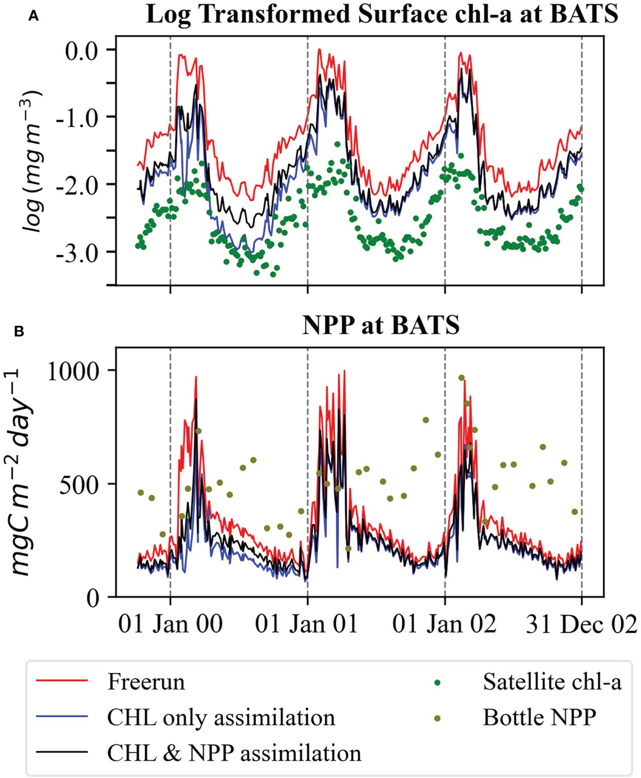
Figure 11 Simulated (A) log-transformed surface chl-a and (B) NPP in the parameter estimation experiments (EXP_{joint_DP)} for free-run, satellite chl-a only assimilation, and simultaneous assimilation of satellite chl-a and in situ NPP.

The photosynthesis parameters α and μ^max have different values at the two stations. Spatial variability of these parameters is due to temperature, nutrient availability, and phytoplankton composition (Bouman et al., 2000). In REcoM2, these parameters are based on the mean values of Geider et al. (1998). In our experiment, the estimated values of α and μ^max for both phytoplankton groups (nanoplankton and diatoms) are within the range of Geider et al. (1998) and other BGC model literature, e.g., Fasham et al. (1990) and Anderson (1993). Similar values were reported at BATS from in situ profiles by Kovač et al. (2018) and in the Mediterranean Sea from a BGC-Argo data by Barbieux et al. (2019).

True values of BGC parameters (if available) are not constant over time and change during seasons (Simon et al., 2015) due to species composition. They also show interannual variability, which is also observed in our experiments. For example, $d_{Nano}^{Chl}$ showed large variability during each assimilation cycle for both stations. Although the overall updates are small, the estimates of the parameter hardly stabilized over the course of the assimilation experiments, indicating a large uncertainty of the parameter with regard to chl-a concentration and NPP simulation. At DYFAMED, the final estimate of the parameter is close to the default value. However, it is quite variable in between and updated at each assimilation cycle. The parameter is less constrained during bloom peak episodes. Intra- and inter-annual variations indicate that time-dependent parameters should be used in ocean BGC models. It also suggests that parameter values resulting from a short period may not be suitable for multi-decadal ecosystem studies or generating long BGC reanalysis.

Although we get similar values of $d_{Nano}^{Chl}$ at BATS, when assimilating only satellite chl-a and by the simultaneous assimilation of satellite chl-a and in situ NPP data, the value of $d_{Nano}^{Chl}$ converges after the second bloom period for the earlier case at both sites. In contrast, simultaneous assimilation leads to time-varying parameter estimates. At DYFAMED, we obtain similar variation over time. However, the change in the parameter value is smaller.

Loss of chlorophyll from functional cells, here described by a chlorophyll degradation rate d^Chl , is a necessary but hard to constrain process in quota-based ecosystem models. The original model by Geider et al. (1998), which primarily describes photoacclimation on timescales of days, contains no such term, which becomes mainly important during low-growth situations in winter and at the lower boundaries of the euphotic zone. Without a chlorophyll loss term, which in reality describes complicated processes in senescent or photostressed cells, phytoplankton C:Chl ratios become unreasonable in such situations. The parameter is therefore usually tuned subjectively until when a reasonable agreement between observation and simulation is found and may not be suitable for BGC models other than those for which they were tuned. A wide range of values of this parameter can led to improvement in the model results as the parameter shows correlation with other parameters (Figure 8). The estimated values resulted from all our joint-estimation experiments are below 0.25. It has been shown (Álvarez et al., 2018) that a replacement of the simple chlorophyll degradation model by a more process-based description of the degradation of photosystem functionality can lead to improvements in modeled C:Chl ratios. This should be pursued further.

In REcoM2, phytoplankton mortality is described by grazing and aggregation. The grazing parameters have large updates in both stations. At BATS, changes in the grazing parameters were prominent, whereas changes in aggregation were prominent at DYFAMED. In REcoM2, the loss process is dominated by aggregation compared with grazing (Laufkötter et al., 2016). However, at BATS, the model overall underestimated NPP compared to the in situ observations but overestimated surface chl-a (see Figure 3). Therefore, to reduce the model-data misfit of NPP and chl-a, the simulation had to keep the phytoplankton population sufficiently low through enhanced grazing. On the other hand, the model overestimated NPP compared to in situ observations, which compensated for more aggregation rather than grazing.

The durations of the spring blooms reproduced by the model and the filter are too short compared to the satellite data (Figure 10). Ensemble members using the default parameters overestimate the chl-a concentration during the bloom periods at BATS. The model state with estimated parameters displays a better fit to the observations at this site. This is an additional indication justifying the increased grazing at BATS. At DYFAMED, on the other hand, the surface chl-a concentration exhibits a better fit to the observations during the bloom period justifying the increased aggregation.

At BATS, the estimated maximum grazing rate of zooplankton ξ exceeds what is commonly considered a “realistic” value in the biogeochemistry literature. Most likely, this parameter compensating for the other grazing parameter, i.e., γ , which indicates large uncertainty of the grazing process at BATS. Including both grazing parameters in the estimation process enabled the model to follow a trajectory that better fits with satellite chl-a concentration and in situ NPP. Satellite chl-a assimilation produces a more reasonable value of γ at BATS (0.61) but increases discrepancies in NPP simulation. Anderson et al. (2015) also used similarly high value of γ and found good agreement between simulation and observation of primary production but at different locations. In addition, more realistic values of both grazing parameters could be obtained by representing phytoplankton mortality as physiological mortality in addition to aggregation as is currently used in REcoM2.

Although sparse in time, the assimilation of in situ NPP had a large impact on the parameter estimates at both sites, particularly at BATS. Parameter estimation with only satellite chl-a assimilation improves the modeled surface chl-a but deteriorates NPP (Figure 11). Assimilation of both satellite chl-a and bottle NPP data improves the NPP prediction by 25% compared with satellite chl-a only assimilation without deteriorating the chl-a prediction. Satellite chl-a data are insufficient to constrain the BGC parameters although they are closely related. However, ¹⁴C primary production shows large discrepancies with satellite-based estimations as discussed in Section 4.3.

We found correlations between some of the parameters that preclude those parameters from being estimated independently. Correlation between parameters can prevent estimating realistic parameter values. Co-dependencies between parameters mean that different sets of parameter values can be optimal. This suggests that BGC models have no single optimal configuration. Therefore, model parameters cannot be meaningfully “tuned” without additional conditions.

Some studies noted that BGC parameters often could not be effectively constrained, especially in high-dimensional cases when many parameters are considered together (Ward et al., 2010; Fiechter et al., 2013; Ward et al., 2013) due to the lack of available observations or specific types of observations. The optimal value of each parameter can depend on other variables that we have not assimilated. Although we have reduced the model-data misfit substantially, correlations among parameters and dependence on other state variables lead to uncertainties in the estimated values of some parameters.

By perturbing 10 selected parameters and updating them to bring the model close to observations, we assume that the remaining BGC parameters do not contribute to the model uncertainty. However, the existing knowledge of the BGC parameter uncertainties and their covariances is not sufficient to define a subset of parameters that is optimal. In this study, we assessed how uncertainties in a limited set of parameters are related to each other. Some of our results may depend upon the subset of parameters chosen for perturbation. Different combinations of parameters might lead to better model estimates than others. The covariances of BGC parameter uncertainties will need to be further explored.

4.2 Usefulness of estimated parameters

In Section 3.2, we presented that the estimated parameters improved the prediction capability of REcoM2 substantially. However, limitations remain depending on the purpose of their use. One limitation is that parameter estimation experiments were conducted for 3 years. Thus, the improved parameters may not be optimal for long-term climate simulations/projections. Furthermore, the parameters varied over time, and not all parameters converged to a constant value. Using the values from the end of the parameter estimation experiments as parameters for the subsequent experiments showed improved model skill. Nonetheless, it is not clear whether these values are the optimal choices.

An alternative to the parameter values at the end of the experiments is to take time averaged values over some later part of the experiment as estimated parameters. However, not all BGC parameters converge during the parameter estimation experiment. For example, α_nano and γ do not have any clear convergence at BATS even after 3 years of DA. We also performed an experiment using the estimated parameters averaged over the entire period of the DA experiment. The parameter values taken at the end of the experiments outperform the time-averaged parameter estimates. This also raises the question of the optimal length of the experiment, which is hard, if not impossible, to define. The 3-year period used in our experiments repeatedly covers the bloom and non-bloom seasons that should be sufficient for the parameter estimation. In our experiment, some parameters did not converge. For these parameters, optimal values might vary in time in order to react to varying growth conditions.

We estimated parameters in two different locations and found distinct optimal parameter values. This points to the fact that BGC parameters can vary substantially across space dependent of physical and ecosystem context. This implies that regional and global 3-D models should profit from using spatially varying parameter values. The methods that we used here to estimate parameters can be extended to estimate spatially varying parameter values in a 3-D model. For this, each parameter has to be defined as a 3-D field that then can be estimated utilizing the cross covariances with the observation analogous to the 1-D setup.

The existence of correlations between some parameters indicates that there is no single combination of model parameters that can be considered to be optimal. This means that predictions of a single model configuration are likely to underestimate the magnitude of the uncertainty around the best estimates. Using an ensemble with perturbed parameters will help to represent this uncertainty.

In addition, we did not consider the uncertainty of the physical simulations in this study. It is possible that BGC parameters also compensate for uncertainties from model physics. Whereas ensemble-based DA would allow us to quantify uncertainty in model parameters, in the structure, and in the forcing data used to compute the model predictions, the experiments implemented here focused only on parameter uncertainty and did not allow for quantification of uncertainty in the physical simulations.

4.3 Discrepancies of bottle NPP data at BATS

In situ bottle NPP has large discrepancies with model predictions (Figure 9). At BATS, in situ NPP shows no prominent seasonality, at least for the period of our experiments. We further explored the satellite-derived NPP estimation based on the CAFE model. We compared the monthly mean satellite-derived NPP with the monthly mean NPP resulting from the state estimation experiment with estimated parameters (EXP_{State_EP}) and in situ bottle data at BATS. Both model and satellite data show a clear seasonal cycle, whereas in situ bottle data are rather erratic (Figure 12). Tin et al. (2016) also found that satellite-based estimation captures the strong seasonality. In contrast, in situ data show more variability due to errors in the measurement. Saba et al. (2010) found that ocean BGC models underestimate the NPP at BATS.

FIGURE 12

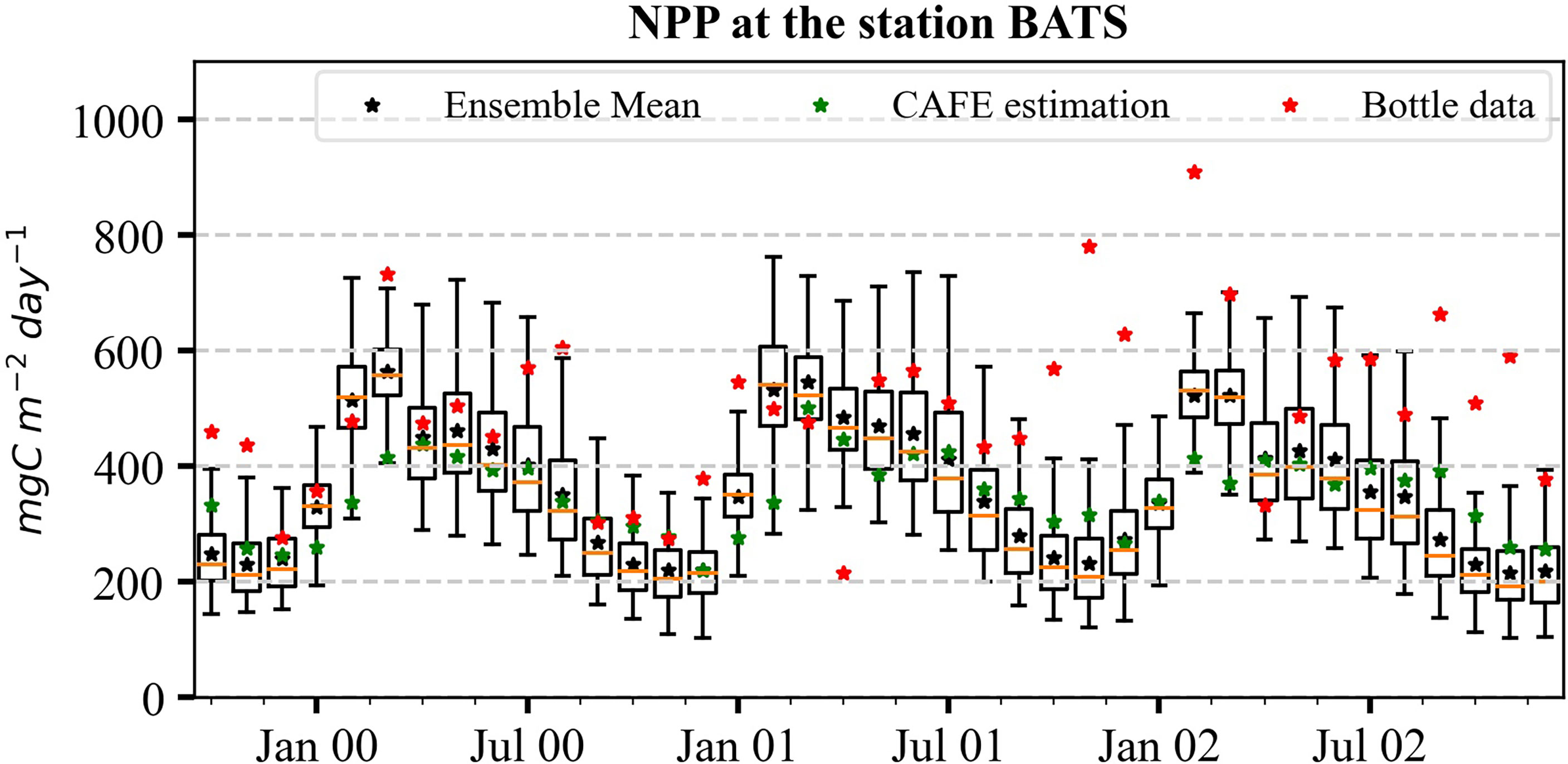
Figure 12 Comparison of monthly mean simulated NPP of EXP_{State_EP}, satellite-derived NPP based on SeaWiFS satellite and in situ bottle data. The box denotes the lower to upper quartile values of ensemble members. The horizontal line on the box is the median of the ensemble. The whiskers show the range of the ensemble.

Another explanation for the large model-data misfit at BATS is the absence of picoplankton in REcoM2, which causes the increase in phytoplankton biomass in the summer (White et al., 2015). At BATS, picoplankton dominates the phytoplankton community during the off-peak period and becomes abundant in late spring to early winter but is usually scarce during the bloom period (Steinberg et al., 2001). Furthermore, the productivity of picoplankton is higher than other phytoplankton in the western Sargasso Sea (Malone et al., 1993) and is sensitive to nitrogen limitation. In summer and fall, when the thermocline is shallow (deep nitracline), nitrogen levels (Nitrate + Nitrite) go below 80 m from the surface. Therefore, picoplankton grows in the deeper part of the euphotic zone (DuRand et al., 2001). Another possibility is that, in fall, when deep mixing does not occur, the temperature of the euphotic zone rises and picoplankton grows deep in the water column below the euphotic zone (Fawcett et al., 2014). Thus, picoplankton has a greater impact on deep chlorophyll maximum (DCM) during the off-peak period, which is not represented in REcoM2. Therefore, REcoM2 may underestimate the total NPP in picoplankton-dominated regions.

A DCM is a common feature that occurs below the mixed layer in the oligotrophic ocean. We further investigate the vertical profile of chl-a concentrations for the existence of a DCM layer (DCML) at BATS. As can be seen in Figure 13, the simulated depths of DCML are shallower than the observed DCML during the off-peak periods. DA application did not change the DCML and the vertical structure of the chl-a profile much. Any deepening in DCML should reflect NPP increases. The observed DCML peaks between 60 and 120 m (Figure 13), indicating active picoplankton production during the off-peak period at BATS, which is absent in the model. High surface chl-a concentrations in spring are associated with deep convective mixing, which leads to a shallower DCML. At BATS, most of the phytoplankton groups increase during bloom periods rather than any single group (Steinberg et al., 2001). This suggests that the picoplankton grows above the euphotic zone during the bloom period at BATS. However, during the off-peak period, the most important biomass component of the DCML is picoplankton, which the model does not represent. This could also explain the underestimation of NPP at BATS by REcoM2.

FIGURE 13

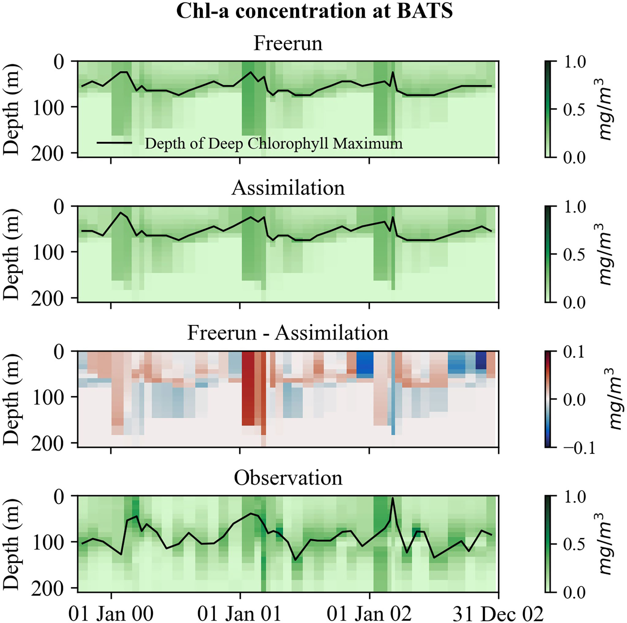
Figure 13 Simulations of chl-a concentration of EXP_{State_EP} at BATS. The black solid lines represent DCML.

5 Conclusions

In this study, we estimated the values of 10 preselected parameters of the BGC model REcoM2 and evaluated the effectiveness of the estimated parameters on the predictive performance of the model, including the uncertainty quantification of the parameters at two BGC time-series stations: BATS and DYFAMED. The parameters characterize the major processes of phytoplankton sources and sinks, such as photosynthesis, chlorophyll degradation, grazing, and aggregation. We used a 1-D configuration of the coupled MITgcm-REcoM2 model and assimilated 5-day satellite chl-a concentration and monthly in situ NPP for 3 years at both sites applying the ESTKF, an ensemble square root filter. The estimated parameters were assessed and found to improve the prediction capability and the seasonal variability of the model simulations.

The parameter estimation procedure generated improved parameter values when satellite chl-a and in situ NPP data were simultaneously assimilated. Assimilating satellite chl-a data alone did not adequately constrain the model. In this case, the filter adjusted the model toward optimal chl-a simulations. However, it generated parameter values that resulted in larger model-data misfits for NPP. We also found large discrepancies in situ NPP data, which may arise not only from the ¹⁴C methodology but also from the distribution of particles and organisms in the highly oligotrophic BATS and DYFAMED waters (Harris et al., 1989).

The strongest updates of the parameters happen during the spring blooms at both stations. As the spring bloom intensity at BATS is lower than at DYFAMED, the pattern of changes in the parameters at BATS is more irregular, not only in one season but throughout the entire assimilation period. As expected, the parameter update is strongly linked to the bias in the estimates of the state variables. Given the large bias in surface chl-a at BATS, some parameters (e.g., α_nano and γ) may be subject to changes even after 3 years of assimilation, whereas at DYFAMED, we obtained more stable parameter values. The contribution of diatoms in the phytoplankton community is larger at BATS than at DYFAMED. This complements our finding that grazing parameters are more important than aggregation for describing phytoplankton mortality at BATS.

We found that dependences between some parameters exist—a change in one parameter affects the evolution of others. This behavior indicates that multiple different combinations of parameter values are possible, and therefore, they cannot be estimated independently. It further suggests that BGC models have no single optimal configuration and predictions from single model configuration are likely to underestimate the magnitude of the uncertainty around the best estimates. The solution is to design ensemble modeling approaches using a sufficiently large ensemble with perturbed parameters.

Given the high parameter uncertainty of BGC models, parameter estimation is essential. However, the model simulations depend on the parameter values in non-linear ways and vary spatially and temporally, which requires a systematic examination of parameters in time and space. Estimating spatial and temporal varying parameter values will allow for efficient exploration of BGC process and modeling at the basin and global level. We point out that the method and learning from this study will serve as an important base for conducting spatially and temporally varying ocean BGC parameter estimation studies at the global level. Estimation of spatially and temporally varying parameter values in a 3-D global ocean BGC model will be considered in future studies.

Data availability statement

Publicly available datasets were analyzed in this study. The Bermuda Atlantic Time-series Study (BATS) station dataset is available at http://bats.bios.edu/. Dynamique des Flux Atmosphériques en Méditerranée (DYFAMED) station dataset is available at https://www.seanoe.org/data/00326/43749/. The Ocean Color Climate Change Initiative (OC-CCI) dataset is available at https://www.oceancolour.org/. The model outputs are available on request to the corresponding author.

Author contributions

All authors—NM, CV, MV, and LN—contributed to conceptualizing, defining experiments, and analyzing outputs. NM carried out the experiments and drafted the manuscript. CV, MV, and LN contributed improving the manuscript draft. LN acquired the funding. All authors contributed to the article and approved the submitted version.

Funding

This study was supported by the Helmholtz Initiative and Networking Fund pilot project Uncertainty Quantification – From Data to Reliable Knowledge (Helmholtz-UQ).

Acknowledgments

We acknowledge the Open Access funding enabled and organized by the Alfred-Wegener-Institut (AWI) Open Access Fund.

Conflict of interest

The authors declare that the research was conducted in the absence of any commercial or financial relationships that could be construed as a potential conflict of interest.

Publisher’s note

All claims expressed in this article are solely those of the authors and do not necessarily represent those of their affiliated organizations, or those of the publisher, the editors and the reviewers. Any product that may be evaluated in this article, or claim that may be made by its manufacturer, is not guaranteed or endorsed by the publisher.

Supplementary material

The Supplementary Material for this article can be found online at: https://www.frontiersin.org/articles/10.3389/fmars.2022.984236/full#supplementary-material

References

Albani S., Mahowald N. M., Perry A. T., Scanza R. A., Zender C. S., Heavens N. G., et al. (2014). Improved dust representation in the community atmosphere model. J. Adv. Modeling Earth Syst. 6 (3), 541–570. doi: 10.1002/2013ms000279

CrossRef Full Text | Google Scholar

Álvarez E., Thoms S., Völker C. (2018). Chlorophyll to carbon ratio derived from a global ecosystem model with photodamage. Global Biogeochemical Cycles 32 (5), 799–816. doi: 10.1029/2017gb005850

CrossRef Full Text | Google Scholar

Anderson T. R. (1993). A spectrally averaged model of light penetration and photosynthesis. Limnology Oceanography 38 (7), 1403–1419. doi: 10.4319/lo.1993.38.7.1403

CrossRef Full Text | Google Scholar

Anderson J. L. (2001). An ensemble adjustment kalman filter for data assimilation. Monthly Weather Rev. 129 (12), 2884–2903. doi: 10.1175/1520-0493(2001)129<2884:AEAKFF>2.0.CO;2

CrossRef Full Text | Google Scholar

Anderson T. R., Gentleman W. C., Yool A. (2015). EMPOWER-1.0: An efficient model of planktonic ecOsystems WrittEn in r. Geoscientific Model. Dev. 8 (7), 2231–2262. doi: 10.5194/gmd-8-2231-2015

CrossRef Full Text | Google Scholar

Bagniewski W., Fennel K., Perry M. J., D'Asaro E. A. (2011). Optimizing models of the north Atlantic spring bloom using physical, chemical and bio-optical observations from a Lagrangian float. Biogeosciences 8 (5), 1291–1307. doi: 10.5194/bg-8-1291-2011

CrossRef Full Text | Google Scholar

Barbieux M., Uitz J., Gentili B., Pasqueron de Fommervault O., Mignot A., Poteau A., et al. (2019). Bio-optical characterization of subsurface chlorophyll maxima in the Mediterranean Sea from a biogeochemical-argo float database. Biogeosciences 16 (6), 1321–1342. doi: 10.5194/bg-16-1321-2019

CrossRef Full Text | Google Scholar

BATS Team (2020). Available at: http://bats.bios.edu/ (Accessed June 2021). Online.

Google Scholar

Béthoux J. P., Morin P., Chaumery C., Connan O., Gentili B., Ruiz-Pino D. (1998). Nutrients in the Mediterranean Sea, mass balance and statistical analysis of concentrations with respect to environmental change. Mar. Chem. 63 (1), 155–169. doi: 10.1016/S0304-4203(98)00059-0

CrossRef Full Text | Google Scholar

Bouman H. A., Platt T., Kraay G. W., Sathyendranath S., Irwin B. D. (2000). Bio-optical properties of the subtropical north atlantic. i. vertical variability. Mar. Ecol. Prog. Ser. 200, 3–18. doi: 10.3354/meps200003

CrossRef Full Text | Google Scholar

Boyle E. A., Anderson R. F., Cutter G. A., Fine R., Jenkins W. J., Saito M. (2015). Introduction to the U.S. GEOTRACES north Atlantic transect (GA-03): USGT10 and USGT11 cruises. Deep Sea Res. Part II: Topical Stud. Oceanography 116, 1–5. doi: 10.1016/j.dsr2.2015.02.031

CrossRef Full Text | Google Scholar

Brown P. T., Caldeira K. (2017). Greater future global warming inferred from earth's recent energy budget. Nature 552 (7683), 45–50. doi: 10.1038/nature24672

PubMed Abstract | CrossRef Full Text | Google Scholar

Campbell J. W. (1995). The lognormal distribution as a model for bio-optical variability in the sea. J. Geophysical Res. 100 (C7). doi: 10.1029/95jc00458

CrossRef Full Text | Google Scholar

Carroll D., Menemenlis D., Adkins J. F., Bowman K. W., Brix H., Dutkiewicz S., et al. (2020). The ECCO-Darwin data-assimilative global ocean biogeochemistry model: Estimates of seasonal to multidecadal surface ocean p CO₂ and air-Sea CO₂ flux. J. Adv. Modeling Earth Syst. 12 (10), e2019MS001888. doi: 10.1029/2019ms001888

CrossRef Full Text | Google Scholar

Ciavatta S., Brewin R. J. W., Skakala J., Polimene L., de Mora L., Artioli Y., et al. (2018). Assimilation of ocean-color plankton functional types to improve marine ecosystem simulations. J. Geophysical Research-Oceans 123 (2), 834–854. doi: 10.1002/2017jc013490

CrossRef Full Text | Google Scholar

Ciavatta S., Kay S., Saux-Picart S., Butenschon M., Allen J. I. (2016). Decadal reanalysis of biogeochemical indicators and fluxes in the north West European shelf-sea ecosystem. J. Geophysical Research-Oceans 121 (3), 1824–1845. doi: 10.1002/2015jc011496

CrossRef Full Text | Google Scholar

Ciavatta S., Torres R., Martinez-Vicente V., Smyth T., Dall'Olmo G., Polimene L., et al. (2014). Assimilation of remotely-sensed optical properties to improve marine biogeochemistry modelling. Prog. Oceanography 127, 74–95. doi: 10.1016/j.pocean.2014.06.002

CrossRef Full Text | Google Scholar

Coppola L., Diamond R. E., Carval T. (2021). Dyfamed observatory data (SEANOE). Available at: https://www.seanoe.org/data/00326/43749/.

Google Scholar

de Fommervault O. P., Migon C., D׳Ortenzio F., Ribera d'Alcalà M., Coppola L. (2015). Temporal variability of nutrient concentrations in the northwestern Mediterranean sea (DYFAMED time-series station). Deep Sea Res. Part I: Oceanographic Res. Papers 100, 1–12. doi: 10.1016/j.dsr.2015.02.006

CrossRef Full Text | Google Scholar

Doron M., Brasseur P., Brankart J. M., Losa S. N., Melet A. (2013). Stochastic estimation of biogeochemical parameters from globcolour ocean colour satellite data in a north Atlantic 3D ocean coupled physical-biogeochemical model. J. Mar. Syst. 117, 81–95. doi: 10.1016/j.jmarsys.2013.02.007

CrossRef Full Text | Google Scholar

Droop M. R. (1983). 25 years of algal growth-kinetics - a personal view. Botanica Marina 26 (3), 99–112. doi: 10.1515/botm.1983.26.3.99

CrossRef Full Text | Google Scholar

DuRand M. D., Olson R. J., Chisholm S. W. (2001). Phytoplankton population dynamics at the Bermuda Atlantic time-series station in the Sargasso Sea. Deep-Sea Res. Part II-Topical Stud. Oceanography 48 (8-9), 1983–2003. doi: 10.1016/S0967-0645(00)00166-1

CrossRef Full Text | Google Scholar

European Space Agency (2021). Available at: https://www.oceancolour.org/ (Accessed June 14 2021). Online.

Google Scholar

Falkowski P. G. (1981). Light-shade adaptation and assimilation numbers. J. Plankton Res. 3 (2), 203–216. doi: 10.1093/plankt/3.2.203

CrossRef Full Text | Google Scholar

Fasham M. J. R., Ducklow H. W., McKelvie S. M. (1990). A nitrogen-based model of plankton dynamics in the oceanic mixed layer. J. Mar. Res. 48 (3), 591–639. doi: 10.1357/002224090784984678

CrossRef Full Text | Google Scholar

Fawcett S. E., Lomas M. W., Ward B. B., Sigman D. M. (2014). The counterintuitive effect of summer-to-fall mixed layer deepening on eukaryotic new production in the Sargasso Sea. Global Biogeochemical Cycles 28 (2), 86–102. doi: 10.1002/2013gb004579

CrossRef Full Text | Google Scholar

Fennel K., Gehlen M., Brasseur P., Brown C. W., Ciavatta S., Cossarini G., et al. (2019). Advancing marine biogeochemical and ecosystem reanalyses and forecasts as tools for monitoring and managing ecosystem health. Front. Mar. Sci. 6. doi: 10.3389/fmars.2019.00089

CrossRef Full Text | Google Scholar

Fennel K., Losch M., Schroter J., Wenzel M. (2001). Testing a marine ecosystem model: sensitivity analysis and parameter optimization. J. Mar. Syst. 28 (1-2), 45–63. doi: 10.1016/S0924-7963(00)00083-X

CrossRef Full Text | Google Scholar

Fiechter J., Broquet G., Moore A. M., Arango H. G. (2011). A data assimilative, coupled physical-biological model for the coastal gulf of Alaska. Dynamics Atmospheres Oceans 52 (1-2), 95–118. doi: 10.1016/j.dynatmoce.2011.01.002

CrossRef Full Text | Google Scholar

Fiechter J., Herbei R., Leeds W., Brown J., Milliff R., Wikle C., et al. (2013). A Bayesian parameter estimation method applied to a marine ecosystem model for the coastal gulf of Alaska. Ecol. Model. 258, 122–133. doi: 10.1016/j.ecolmodel.2013.03.003

CrossRef Full Text | Google Scholar

Flato G. M. (2011). Earth system models: an overview. Wiley Interdiscip. Reviews-Climate Change 2 (6), 783–800. doi: 10.1002/wcc.148

CrossRef Full Text | Google Scholar

Flynn K. J., McGillicuddy D. J. (2018). "Modeling Marine Harmful Algal Blooms: Current Status and Future Prospects," in Harmful Algal Blooms: A Compendium Desk Reference, eds. Shumway S. E., Burkholder J. M., Morton S. L. (Hoboken, New Jersey: Wiley-Blackwell). pp. 115–134. doi: 10.1002/9781118994672.ch3

CrossRef Full Text | Google Scholar

Friedrichs M. A. M. (2001). Assimilation of JGOFS EqPac and SeaWiFS data into a marine ecosystem model of the central equatorial pacific ocean. Deep-Sea Res. Part II -Topical Stud. Oceanography 49 (1-3), 289–319. doi: 10.1016/s0967-0645(01)00104-7

CrossRef Full Text | Google Scholar

Friedrichs M. A. M., Dusenberry J. A., Anderson L. A., Armstrong R. A., Chai F., Christian J. R., et al. (2007). Assessment of skill and portability in regional marine biogeochemical models: Role of multiple planktonic groups. J. Geophysical Research-Oceans 112 (C8), C08001. doi: 10.1029/2006jc003852

CrossRef Full Text | Google Scholar

Friedrichs M. A. M., Hood R. R., Wiggert J. D. (2006). Ecosystem model complexity versus physical forcing: Quantification of their relative impact with assimilated Arabian Sea data. Deep-Sea Res. Part II-Topical Stud. Oceanography 53 (5-7), 576–600. doi: 10.1016/j.dsr2.2006.01.026

CrossRef Full Text | Google Scholar

Gehlen M., Barciela R., Bertino L., Brasseur P., Butenschon M., Chai F., et al. (2015). Building the capacity for forecasting marine biogeochemistry and ecosystems: Recent advances and future developments. J. Operational Oceanography 8 (sup1), S168–S187. doi: 10.1080/1755876x.2015.1022350

CrossRef Full Text | Google Scholar

Geider R. J., La Roche J. (1994). The role of iron in phytoplankton photosynthesis, and the potential for iron-limitation of primary productivity in the sea. Photosynth Res. 39 (3), 275–301. doi: 10.1007/BF00014588

PubMed Abstract | CrossRef Full Text | Google Scholar

Geider R. J., MacIntyre H. L., Kana T. M. (1998). A dynamic regulatory model of phytoplanktonic acclimation to light, nutrients, and temperature. Limnology Oceanography 43 (4), 679–694. doi: 10.4319/lo.1998.43.4.0679

CrossRef Full Text | Google Scholar

Gharamti M. E., Samuelsen A., Bertino L., Simon E., Korosov A., Daewel U. (2017a). Online tuning of ocean biogeochemical model parameters using ensemble estimation techniques: Application to a one-dimensional model in the north Atlantic. J. Mar. Syst. 168, 1–16. doi: 10.1016/j.jmarsys.2016.12.003

CrossRef Full Text | Google Scholar

Gharamti M. E., Tjiputra J., Bethke I., Samuelsen A., Skjelvan I., Bentsen M., et al. (2017b). Ensemble data assimilation for ocean biogeochemical state and parameter estimation at different sites. Ocean Model. 112, 65–89. doi: 10.1016/j.ocemod.2017.02.006

CrossRef Full Text | Google Scholar

Goodliff M., Bruening T., Schwichtenberg F., Li X., Lindenthal A., Lorkowski I., et al. (2019). Temperature assimilation into a coastal ocean-biogeochemical model: Assessment of weakly and strongly coupled data assimilation. Ocean Dynamics 69 (10), 1217–1237. doi: 10.1007/s10236-019-01299-7

CrossRef Full Text | Google Scholar

Guieu C., Blain S. (2013). Concentrations of total dissolved iron measured on water bottle samples during THALASSA cruise PROSOPE. PANGAEA. doi: 10.1594/PANGAEA.805278

CrossRef Full Text | Google Scholar

Harris G. P., Griffiths F. B., Thomas D. P. (1989). Light and dark uptake and loss of 14C: Methodological problems with productivity measurements in oceanic waters. Hydrobiologia 173 (2), 95–105. doi: 10.1007/bf00015519

CrossRef Full Text | Google Scholar

Hauck J., Volker C., Wang T., Hoppema M., Losch M., Wolf-Gladrow D. A. (2013). Seasonally different carbon flux changes in the southern ocean in response to the southern annular mode. Global Biogeochem Cycles 27 (4), 1236–1245. doi: 10.1002/2013GB004600

PubMed Abstract | CrossRef Full Text | Google Scholar

Hersbach H., Bell B., Berrisford P., Hirahara S., Horányi A., Muñoz-Sabater J., et al. (2020). The ERA5 global reanalysis. Q. J. R. Meteorol. Soc. 146 (730), 1999–2049. doi: 10.1002/qj.3803

CrossRef Full Text | Google Scholar

Hohn S. (2009). Coupling and decoupling of biogeochemical cycles in marine ecosystems. [dissertation/doctoral thesis]. (Bremen, Germany: Universität Bremen).

Google Scholar

Hoshiba Y., Hirata T., Shigemitsu M., Nakano H., Hashioka T., Masuda Y., et al. (2018). Biological data assimilation for parameter estimation of a phytoplankton functional type model for the western north pacific. Ocean Sci. 14 (3), 371–386. doi: 10.5194/os-14-371-2018

CrossRef Full Text | Google Scholar

Hu J. T., Fennel K., Mattern J. P., Wilkin J. (2012). Data assimilation with a local ensemble kalman filter applied to a three-dimensional biological model of the middle Atlantic bight. J. Mar. Syst. 94, 145–156. doi: 10.1016/j.jmarsys.2011.11.016

CrossRef Full Text | Google Scholar

Hu L. Y., Zhao Y., Liu Y., Scheepens C., Bouchard A. (2013). Updating multipoint simulations using the ensemble kalman filter. Comput. Geosciences 51, 7–15. doi: 10.1016/j.cageo.2012.08.020

CrossRef Full Text | Google Scholar

Jackson G. A., Waite A. M., Boyd P. W. (2005). Role of algal aggregation in vertical carbon export during SOIREE and in other low biomass environments. Geophysical Res. Lett. 32 (13), L13607. doi: 10.1029/2005GL023180

CrossRef Full Text | Google Scholar

JGOFS (1997). “Bermuda Atlantic time-series study (BATS) methods,” in Joint global ocean flux study (JGOFS). Bermuda Biological Station for Research, Inc

Google Scholar

Jones E. M., Baird M. E., Mongin M., Parslow J., Skerratt J., Lovell J., et al. (2016). Use of remote-sensing reflectance to constrain a data assimilating marine biogeochemical model of the great barrier reef. Biogeosciences 13 (23), 6441–6469. doi: 10.5194/bg-13-6441-2016

CrossRef Full Text | Google Scholar

Kane A., Moulin C., Thiria S., Bopp L., Berrada M., Tagliabue A., et al. (2011). Improving the parameters of a global ocean biogeochemical model via variational assimilation of in situ data at five time series stations. J. Geophysical Res. -Oceans 116 (C6), C06011. doi: 10.1029/2009jc006005

CrossRef Full Text | Google Scholar

Kovač Ž., Platt T., Sathyendranath S., Lomas M. (2018). Extraction of photosynthesis parameters from time series measurements of In situ production: Bermuda Atlantic time-series study. Remote Sens. 10 (6), 915. doi: 10.3390/rs10060915

CrossRef Full Text | Google Scholar

Laiolo L., Matear R., Baird M. E., Soja-Wozniak M., Doblin M. A. (2018). Information content of in situ and remotely sensed chlorophyll-a: Learning from size-structured phytoplankton model. J. Mar. Syst. 183, 1–12. doi: 10.1016/j.jmarsys.2018.03.005

CrossRef Full Text | Google Scholar

Large W. G., Yeager S. G. (2008). The global climatology of an interannually varying air–sea flux data set. Climate Dynamics 33 (2-3), 341–364. doi: 10.1007/s00382-008-0441-3

CrossRef Full Text | Google Scholar

Laufkötter C., Vogt M., Gruber N., Aumont O., Bopp L., Doney S. C., et al. (2016). Projected decreases in future marine export production: the role of the carbon flux through the upper ocean ecosystem. Biogeosciences 13 (13), 4023–4047. doi: 10.5194/bg-13-4023-2016

CrossRef Full Text | Google Scholar

Lauvset S. K., Key R. M., Olsen A., van Heuven S., Velo A., Lin X. H., et al. (2016). A new global interior ocean mapped climatology: the 1 degrees x 1 degrees GLODAP version 2. Earth System Sci. Data 8 (2), 325–340. doi: 10.5194/essd-8-325-2016

CrossRef Full Text | Google Scholar

Laws E., Sakshaug E., Babin M., Dandonneau Y., Falkowski P., Geider R., et al. (2002). "Photosynthesis and primary productivity in marine ecosystems: Practical aspects and application of techniques" (Bergen, Norway: Scientific Committee on Oceanic Research and JGOFS International Project Office).

Google Scholar

MacIntyre H. L., Kana T. M., Anning T., Geider R. J. (2002). Photoacclimation of photosynthesis irradiance response curves and photosynthetic pigments in microalgae and cyanobacteria. J. Phycology 38 (1), 17–38. doi: 10.1046/j.1529-8817.2002.00094.x

CrossRef Full Text | Google Scholar

Malone T. C., Pike S. E., Conley D. J. (1993). Transient variations in phytoplankton productivity at the JGOFS Bermuda time series station. Deep Sea Res. Part I: Oceanographic Res. Papers 40 (5), 903–924. doi: 10.1016/0967-0637(93)90080-M

CrossRef Full Text | Google Scholar

Marshall J., Adcroft A., Hill C., Perelman L., Heisey C. (1997). A finite-volume, incompressible navier stokes model for studies of the ocean on parallel computers. J. Geophysical Research-Oceans 102 (C3), 5753–5766. doi: 10.1029/96jc02775

CrossRef Full Text | Google Scholar

Marty J. C. (2002). ). the DYFAMED time-series program (French-JGOFS). Deep-Sea Res. Part II -Topical Stud. Oceanography 49 (11), 1963–1964. doi: 10.1016/S0967-0645(02)00021-8

CrossRef Full Text | Google Scholar

Marty J. C., Chiaverini J. (2010). Hydrological changes in the ligurian Sea (NW Mediterranean, DYFAMED site) during 1995-2007 and biogeochemical consequences. Biogeosciences 7 (7), 2117–2128. doi: 10.5194/bg-7-2117-2010

CrossRef Full Text | Google Scholar

Marty J.-C., Garcia N., Raimbault P. (2008). Phytoplankton dynamics and primary production under late summer conditions in the NW Mediterranean Sea. Deep Sea Res. Part I: Oceanographic Res. Papers 55 (9), 1131–1149. doi: 10.1016/j.dsr.2008.05.001

CrossRef Full Text | Google Scholar

Mattern J. P., Dowd M., Fennel K. (2010). Sequential data assimilation applied to a physical-biological model for the Bermuda Atlantic time series station. J. Mar. Syst. 79 (1-2), 144–156. doi: 10.1016/j.jmarsys.2009.08.004

CrossRef Full Text | Google Scholar

Mattern J. P., Edwards C. A. (2017). Simple parameter estimation for complex models - testing evolutionary techniques on 3-dimensional biogeochemical ocean models. J. Mar. Syst. 165, 139–152. doi: 10.1016/j.jmarsys.2016.10.012

CrossRef Full Text | Google Scholar

Mayot N., Nival P., Levy M. (2020). “Primary production in the ligurian Sea,” in The Mediterranean Sea in the Era of Global Change 1: 30 Years of Multidisciplinary Study of the Ligurian Sea, eds. Migon C., Nival P., Sciandra A.. (Weinheim, Germany: Wiley-VCH GmbH) 139–164.

Google Scholar

McCave I. N. (1984). Size spectra and aggregation of suspended particles in the deep ocean. Deep-Sea Res. Part a-Oceanographic Res. Papers 31 (4), 329–352. doi: 10.1016/0198-0149(84)90088-8

CrossRef Full Text | Google Scholar

McDonald C. P., Bennington V., Urban N. R., McKinley G. A. (2012). 1-d test-bed calibration of a 3-d lake superior biogeochemical model. Ecol. Model. 225, 115–126. doi: 10.1016/j.ecolmodel.2011.11.021

CrossRef Full Text | Google Scholar

Moradkhani H., Hsu K. L., Gupta H., Sorooshian S. (2005). Uncertainty assessment of hydrologic model states and parameters: Sequential data assimilation using the particle filter. Water Resour. Res. 41 (5), W05012. doi: 10.1029/2004wr003604

CrossRef Full Text | Google Scholar

Natvik L. J., Evensen G. (2003). Assimilation of ocean colour data into a biochemical model of the north Atlantic - part 1. data assimilation experiments. J. Mar. Syst. 40, 127–153. doi: 10.1016/S0924-7963(03)00016-2

CrossRef Full Text | Google Scholar

Nelson D. M., Brzezinski M. A. (1997). Diatom growth and productivity in an oligo-trophic midocean gyre: A 3-yr record from the Sargasso Sea near Bermuda. Limnology Oceanography 42 (3), 473–486. doi: 10.4319/lo.1997.42.3.0473

CrossRef Full Text | Google Scholar

Nerger L., Gregg W. W. (2007). Assimilation of SeaWiFS data into a global ocean-biogeochemical model using a local SEIK filter. J. Mar. Syst. 68 (1-2), 237–254. doi: 10.1016/j.jmarsys.2006.11.009

CrossRef Full Text | Google Scholar

Nerger L., Gregg W. W. (2008). Improving assimilation of SeaWiFS data by the application of bias correction with a local SEIK filter. J. Mar. Syst. 73 (1-2), 87–102. doi: 10.1016/j.jmarsys.2007.09.007

CrossRef Full Text | Google Scholar

Nerger L., Hiller W. (2013). Software for ensemble-based data assimilation systems-implementation strategies and scalability. Comput. Geosciences 55, 110–118. doi: 10.1016/j.cageo.2012.03.026

CrossRef Full Text | Google Scholar

Nerger L., Janjic T., Schroter J., Hiller W. (2012). A regulated localization scheme for ensemble-based kalman filters. Q. J. R. Meteorological Soc. 138 (664), 802–812. doi: 10.1002/qj.945

CrossRef Full Text | Google Scholar

Ocean Productivity (2021). http://sites.science.oregonstate.edu/ocean.productivity/index.php [Online]. [Accessed January 10 2022].

Google Scholar

O'Neill R. V., DeAngelis D. L., Pastor J. J., Jackson B. J., Post W. M. (1989). Multiple nutrient limitations in ecological models. Ecol. Model. 46 (3-4), 147–163. doi: 10.1016/0304-3800(89)90015-x

CrossRef Full Text | Google Scholar

Orr J. C., Najjar R. G., Aumont O., Bopp L., Bullister J. L., Danabasoglu G., et al. (2017). Biogeochemical protocols and diagnostics for the CMIP6 ocean model intercomparison project (OMIP). Geoscientific Model. Dev. 10 (6), 2169–2199. doi: 10.5194/gmd-10-2169-2017

CrossRef Full Text | Google Scholar

Pathiraja S., Moradkhani H., Marshall L., Sharma A., Geenens G. (2018). Data-driven model uncertainty estimation in hydrologic data assimilation. Water Resour. Res. 54 (2), 1252–1280. doi: 10.1002/2018wr022627

CrossRef Full Text | Google Scholar

Pelc J. S., Simon E., Bertino L., El Serafy G., Heemink A. W. (2012). Application of model reduced 4D-var to a 1D ecosystem model. Ocean Model. 57-58, 43–58. doi: 10.1016/j.ocemod.2012.09.003

CrossRef Full Text | Google Scholar

Pradhan H. K., Volker C., Losa S. N., Bracher A., Nerger L. (2019). Assimilation of global total chlorophyll OC-CCI data and its impact on individual phytoplankton fields. J. Geophysical Res. - Oceans 124 (1), 470–490. doi: 10.1029/2018jc014329

CrossRef Full Text | Google Scholar

Pradhan H. K., Volker C., Losa S. N., Bracher A., Nerger L. (2020). Global assimilation of ocean-color data of phytoplankton functional types: Impact of different data sets. J. Geophysical Res. - Oceans 125 (2), e2019JC015586. doi: 10.1029/2019JC015586

CrossRef Full Text | Google Scholar

Richardson K., Bendtsen J., Kragh T., Mousing E. A. (2016). Constraining the distribution of photosynthetic parameters in the global ocean. Front. Mar. Sci. 3. doi: 10.3389/fmars.2016.00269

CrossRef Full Text | Google Scholar

Saba V. S., Friedrichs M. A. M., Carr M. E., Antoine D., Armstrong R. A., Asanuma I., et al. (2010). Challenges of modeling depth-integrated marine primary productivity over multiple decades: A case study at BATS and HOT. Global Biogeochemical Cycles 24, GB3020. doi: 10.1029/2009gb003655

CrossRef Full Text | Google Scholar

Sathyendranath S., Brewin R. J. W., Brockmann C., Brotas V., Calton B., Chuprin A., et al. (2019). An ocean-colour time series for use in climate studies: The experience of the ocean-colour climate change initiative (OC-CCI). Sensors (Basel) 19 (19), 4285. doi: 10.3390/s19194285

CrossRef Full Text | Google Scholar

Schartau M., Wallhead P., Hemmings J., Loptien U., Kriest I., Krishna S., et al. (2017). Reviews and syntheses: Parameter identification in marine planktonic ecosystem modelling. Biogeosciences 14 (6), 1647–1701. doi: 10.5194/bg-14-1647-2017

CrossRef Full Text | Google Scholar

Schourup-Kristensen V., Sidorenko D., Wolf-Gladrow D. A., Völker C. (2014). A skill assessment of the biogeochemical model REcoM2 coupled to the finite element Sea ice–ocean model (FESOM 1.3). Geoscientific Model. Dev. 7 (6), 2769–2802. doi: 10.5194/gmd-7-2769-2014

CrossRef Full Text | Google Scholar

Silsbe G. M., Behrenfeld M. J., Halsey K. H., Milligan A. J., Westberry T. K. (2016). The CAFE model: A net production model for global ocean phytoplankton. Global Biogeochemical Cycles 30 (12), 1756–1777. doi: 10.1002/2016gb005521

CrossRef Full Text | Google Scholar

Simon E., Samuelsen A., Bertino L., Dumont D. (2012). Estimation of positive sum-to-one constrained zooplankton grazing preferences with the DEnKF: A twin experiment. Ocean Sci. 8 (4), 587–602. doi: 10.5194/os-8-587-2012

CrossRef Full Text | Google Scholar

Simon E., Samuelsen A., Bertino L., Mouysset S. (2015). Experiences in multiyear combined state-parameter estimation with an ecosystem model of the north Atlantic and Arctic oceans using the ensemble kalman filter. J. Mar. Syst. 152, 1–17. doi: 10.1016/j.jmarsys.2015.07.004

CrossRef Full Text | Google Scholar

Singh T., Counillon F., Tjiputra J., Wang Y., Gharamti M. E. (2022). Estimation of ocean biogeochemical parameters in an earth system model using the dual one step ahead smoother: A twin experiment. Front. Mar. Sci. 9. doi: 10.3389/fmars.2022.775394

PubMed Abstract | CrossRef Full Text | Google Scholar

Song H., Edwards C. A., Moore A. M., Fiechter J. (2016). Data assimilation in a coupled physical-biogeochemical model of the California current system using an incremental lognormal 4-dimensional variational approach: Part 1-model formulation and biological data assimilation twin experiments. Ocean Model. 106, 131–145. doi: 10.1016/j.ocemod.2016.04.001

CrossRef Full Text | Google Scholar

Steinberg D. K., Carlson C. A., Bates N. R., Johnson R. J., Michaels A. F., Knap A. H. (2001). Overview of the US JGOFS Bermuda Atlantic time-series study (BATS): a decade-scale look at ocean biology and biogeochemistry. Deep Sea Res. Part II: Topical Stud. Oceanography 48 (8-9), 1405–1447. doi: 10.1016/s0967-0645(00)00148-x

CrossRef Full Text | Google Scholar

St-Laurent P., Friedrichs M. A. M., Najjar R. G., Martins D. K., Herrmann M., Miller S. K., et al. (2017). Impacts of atmospheric nitrogen deposition on surface waters of the Western north Atlantic mitigated by multiple feedbacks. J. Geophysical Res. - Oceans 122 (11), 8406–8426. doi: 10.1002/2017jc013072

CrossRef Full Text | Google Scholar

Sweeney E. N., McGillicuddy D. J., Buesseler K. O. (2003). Biogeochemical impacts due to mesoscale eddy activity in the Sargasso Sea as measured at the Bermuda Atlantic time-series study (BATS). Deep Sea Res. Part II: Topical Stud. Oceanography 50 (22), 3017–3039. doi: 10.1016/j.dsr2.2003.07.008

CrossRef Full Text | Google Scholar

Tin H. C., Lomas M. W., Ishizaka J. (2016). Satellite-derived estimates of primary production during the Sargasso Sea winter/spring bloom: Integration of in-situ time-series data and ocean color remote sensing observations. Regional Stud. Mar. Sci. 3, 131–143. doi: 10.1016/j.rsma.2015.07.002

CrossRef Full Text | Google Scholar

Tommasi D., Stock C. A., Hobday A. J., Methot R., Kaplan I. C., Eveson J. P., et al. (2017). Managing living marine resources in a dynamic environment: The role of seasonal to decadal climate forecasts. Prog. Oceanography 152, 15–49. doi: 10.1016/j.pocean.2016.12.011

CrossRef Full Text | Google Scholar

Triantafyllou G., Korres G., Hoteit I., Petihakis G., Banks A. C. (2007). Assimilation of ocean colour data into a biogeochemical flux model of the eastern Mediterranean sea. Ocean Sci. 3 (3), 397–410. doi: 10.5194/os-3-397-2007

CrossRef Full Text | Google Scholar

Vetra-Carvalho S., Van Leeuwen P. J., Nerger L., Barth A., Altaf M. U., Brasseur P., et al. (2018). State-of-the-art stochastic data assimilation methods for high-dimensional non-Gaussian problems. Tellus Ser. a-Dynamic Meteorology Oceanography 70 (1), 1–43. doi: 10.1080/16000870.2018.1445364

CrossRef Full Text | Google Scholar

Wang B., Fennel K., Yu L. Q., Gordon C. (2020). Assessing the value of biogeochemical argo profiles versus ocean color observations for biogeochemical model optimization in the gulf of Mexico. Biogeosciences 17 (15), 4059–4074. doi: 10.5194/bg-17-4059-2020

CrossRef Full Text | Google Scholar

Ward B. A., Friedrichs M. A. M., Anderson T. R., Oschlies A. (2010). Parameter optimisation techniques and the problem of underdetermination in marine biogeochemical models. J. Mar. Syst. 81 (1-2), 34–43. doi: 10.1016/j.jmarsys.2009.12.005

CrossRef Full Text | Google Scholar

Ward B. A., Schartau M., Oschlies A., Martin A. P., Follows M. J., Anderson T. R. (2013). When is a biogeochemical model too complex? objective model reduction and selection for north Atlantic time-series sites. Prog. Oceanography 116, 49–65. doi: 10.1016/j.pocean.2013.06.002

CrossRef Full Text | Google Scholar

White A. E., Letelier R. M., Whitmire A. L., Barone B., Bidigare R. R., Church M. J., et al. (2015). Phenology of particle size distributions and primary productivity in the north pacific subtropical gyre (Station ALOHA). J. Geophys Res. Oceans 120 (11), 7381–7399. doi: 10.1002/2015JC010897

PubMed Abstract | CrossRef Full Text | Google Scholar

Wikle C. K., Berliner L. M. (2007). A Bayesian tutorial for data assimilation. Physica D-Nonlinear Phenomena 230 (1-2), 1–16. doi: 10.1016/j.physd.2006.09.017

CrossRef Full Text | Google Scholar

Xiao Y., Friedrichs M. A. M. (2014a). Using biogeochemical data assimilation to assess the relative skill of multiple ecosystem models in the mid-Atlantic bight: effects of increasing the complexity of the planktonic food web. Biogeosciences 11 (11), 3015–3030. doi: 10.5194/bg-11-3015-2014

CrossRef Full Text | Google Scholar

Xiao Y. J., Friedrichs M. A. M. (2014b). The assimilation of satellite-derived data into a one-dimensional lower trophic level marine ecosystem model. J. Geophysical Res. - Oceans 119 (4), 2691–2712. doi: 10.1002/2013jc009433

CrossRef Full Text | Google Scholar

Zhao L., Wei H., Xu Y., Feng S. (2005). An adjoint data assimilation approach for estimating parameters in a three-dimensional ecosystem model. Ecol. Model. 186 (2), 235–250. doi: 10.1016/j.ecolmodel.2005.01.017

CrossRef Full Text | Google Scholar