 Tao Song
 Runsheng Han
 Fan Meng
 Jiarong Wang1
 Shiqiu Peng
94% of researchers rate our articles as excellent or good
Learn more about the work of our research integrity team to safeguard the quality of each article we publish.
Find out more
ORIGINAL RESEARCH article
Front. Mar. Sci. , 03 October 2022
Sec. Ocean Observation
Volume 9 - 2022 | https://doi.org/10.3389/fmars.2022.983007
This article is part of the Research Topic Spatiotemporal Modeling and Analysis in Marine Science View all 13 articles
Accurate wave height prediction is significant in ports, energy, fisheries, and other offshore operations. In this study, a regional significant wave height prediction model with a high spatial and temporal resolution is proposed based on the ConvLSTM algorithm. The model learns the intrinsic correlations of the data generated by the numerical model, making it possible to combine the correlations between wind and wind waves to improve the predictions. In addition, this study also optimizes the long-term prediction ability of the model through the proposed Mask method and Replace mechanism. The experimental results show that the introduction of the wind field can significantly improve the significant wave height prediction results. The research on the prediction effect of the entire study area and two separate stations shows that the prediction performance of the proposed model is better than the existing methods. The model makes full use of the physical correlation between wind and wind waves, and the validity is up to 24 hours. The 24-hour forecast R² reached 0.69.
Wind waves are waves generated by and influenced by the local wind (Barnett and Kenyon, 1975). It is characterized by often sharp wave crests, very irregular distribution on the sea surface, short crest lines, and minor periods. When the wind is strong, the phenomenon of breaking waves often occurs, and water splashes are formed. In general, wind disturbance of the sea surface causes capillary waves (ripples) so that the wind further provides the necessary roughness for delivering energy to the sea surface. Then, the waves continue to be fueled by the pressure of the wind on its surface (Longuet-Higgins, 1963; Kirby, 1985), causing the wind waves to grow (Phillips, 1957). Wind waves dominate the motion of the sea for a short period. Therefore the study of wind waves has implications for many applications such as navigation safety and coastal engineering. Waves also define air-sea fluxes and interact strongly with surface currents, upper ocean turbulence, and sea ice. Understanding and accurately predicting waves are very beneficial to humans.
In the past few decades, researchers have made great strides in studying the causes of wind waves and the correlation between wind and waves (Barnett, 1968). In order to analyze the wind waves field, Sverdrup and Munk (1947) first used an empirical or semi-analytical approach. However, the method has obvious limitations (Kamranzad et al., 2011). Hasselmann (1968) has also studied the evolution of the wind waves’ power spectrum in-depth and demonstrated a strong correlation between both wind and wind waves.
At this stage, the mainstream forecasting idea for oceanographers to forecast wind waves is to use numerical models. The numerical model uses oceanic elements such as wind as input and solves complex equations to produce wave forecasts. The most widely used models include the National Weather Service’s (NWS) WaveWatch III (WW3) (Tolman et al., 2009), Simulating Waves Nearshore (SWAN) (Booij et al., 1999) developed by the Delft University of Technology, etc (Zheng et al., 2016). Traditional numerical model forecasting methods combine the advantages of physical simulation and data-driven approaches to make forecasts with high spatial and temporal resolution (Wei et al., 2013). This hybrid approach of physical simulation and data-driven prediction is theoretically sound. However, it has significant limitations in practical offshore industry applications: the time lag and its accuracy cannot be guaranteed. In addition, the expensive computational and maintenance costs of the numerical model make it a prudent consideration as an operational application (Song et al., 2022).
In recent years, the application of Artificial Intelligence (AI) in marine and atmospheric sciences has developed rapidly (Van Aartrijk et al., 2002; Bolton and Zanna, 2019). AI can naturally process many data sources, such as numerical forecast results, radar, satellite, station observations, and even decision data (natural language), which is almost impossible for existing coupled sea-air numerical models. Some studies have even found that AI models outperform existing numerical models for short-term wind waves prediction (James et al., 2018). Berbić et al. (2017); Callens et al. (2020) predicted the significant wave height within 3-hour accurately using Random Forest (RF) and Support Vector Machine (SVM), respectively. Fan et al. (2020) used the Long Short Term Memory Network(LSTM) algorithm to predict the significant wave height of several stations for 6-hour, and the results were satisfactory. Song et al. (2020) uses merged-LSTM to mine the hidden patterns in short time series to solve the long-term dependence of series variability and to make compelling predictions of sea surface height anomaly(SSHA). Meng et al. (2021) proposes a bi-directional gated recurrent unit (BiGRU) network for predicting wave heights during tropical cyclones (TCs). Artificial intelligence has the advantage of solid data drive and a high potential for model optimization, which can theoretically solve the “costly” problem of numerical forecast models while improving the “accuracy” of forecasts.
Although the application of AI in wave height prediction is becoming more and more widespread, most of them are limited to single-site forecasting. However, wind wave fields are two-dimensional fields, so predicting wave height at a point is not only a matter of time series but should also consider the spatial correlation with other surrounding points (Jönsson et al., 2003; Gavrikov et al., 2016). In addition, most current AI applications for predicting wave height use single-factor forecasting, treating each ocean variable individually, which ignores the correlation between different ocean elements and lacks physical meaning (Fu et al., 2019). Only the wave field factor is applied to forecast the wave field. The physical correlation between wind and wind waves is ignored. Zhou et al. (2021) established A two-dimensional SWH prediction model based on convolution Long and Short-term memory (ConvLSTM). However, the model only considers the wave and ignores the influence of wind. The mean absolute percentage errors of 6-hour, 12-hour, and 24-hour advance are 15%, 29%, and 61%, respectively. Moreover, the spatial and temporal resolution of the data should also be considered if the deep learning approach is to be truly applied to the problem of forecasting ocean elements. With the deep development of ocean research, human production life increasingly needs to understand the ocean elements with high spatial and temporal resolution. Most of the current deep learning wave forecasting methods are limited to low spatial and temporal resolution conditions, and such research can no longer meet the practical needs of society.
In this study, a deep learning model based on ConvLSTM was developed to combine the correlation between wind and wind waves to predict significant wave heights with high spatial and temporal resolution in the Beibu Gulf. ConvLSTM has been successfully applied to 2D precipitation prediction (Shi et al., 2015). It enables the model to learn the spatial correlation of elements through a unique convolution method, which solves the problem of spatial information loss in traditional LSTM and improves the accuracy of 2D predictions. Specific modifications to the model were made in this study to enable the model to be adapted to the study sea area and to learn the correlation between wind and significant wave heights in the numerical model data. We then set up a series of experiments to evaluate the performance and accuracy of the model. The model successfully predicts the hourly significant wave height of 1/40° and has an excellent long-term prediction ability. After the model is trained, it is only necessary to provide the model with the corresponding wind speed and significant wave height data to obtain the required predicted significant wave height.
The rest of the paper is organized as follows: Section.2 describes the data and research area we used, and Section.3 describes the method used and the construction and evaluation metrics of the proposed model. Section.4 shows the predictive performance of the proposed model and corrects the problems in the prediction process. Finally, we conclude and discuss future research recommendations in Section.5.
In this work, the study area is the Beibu Gulf and its adjacent waters in the South China Sea (16°N - 23°N, 105°E - 113°E), as shown in the black box in Figure 1. It includes the shelf waters as well as other waters around Hainan Island; the water depth gradually deepens from the shore to the central part, with an average depth of 42 meters and a maximum depth of more than 100 meters (Gao et al., 2015). The study area is mainly surrounded by some cities in Guangxi, Guangdong, Hainan Province (China), and Vietnam, which are important ports and good fishing grounds (Koongolla et al., 2020). The Beibu Gulf is located in tropical and subtropical areas (Cooke et al., 2011). In winter, it is influenced by cold air from mainland China, with northeast winds and sea surface temperature of about 20C. In summer, the wind comes from the tropical ocean, mainly from the southwest, and the sea surface temperature is as high as 30C. It is often attacked by typhoons. Generally, about five typhoons (Shao et al., 2018) pass here every year.
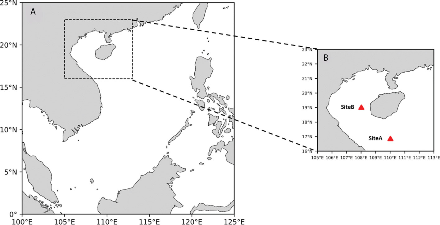
Figure 1 (A) South China Sea and the Beibu Gulf, and (B) Beibu Gulf and its adjacent waters.
The data used in this study are the significant wave height (SWH) and wind speed (WS) data. It is worth noting that the significant wave height data we use refers specifically to the significant wave height of wind waves. These data were provided by the South China Sea Institute of Oceanography, Chinese Academy of Sciences. These data are the products of the WAVEWATCH III and COAM models. The researchers involved have adopted the latest wind stress calculation scheme based on the third-generation wave model WW3, which improves the model’s prediction of wind and waves generated by different wind speeds and wind field variations. The model allows a better simulation of the temporal variation of the waves, and the values obtained are closer to the observed values than in the ERA5 reanalysis. The model can provide hourly forecasts with a spatial resolution of 1/40°*1/40°. A more detailed description of the data is available here (Li et al., 2021). Due to the high accuracy of these data, they can be used as an approximation of the observed data in the case of insufficient actual measurement data. Since it is difficult to obtain actual measurement data with high accuracy in the study area, we used the above data as a comparison value in our study. In this study, SWH and WS data with Spatio-temporal resolution of 1h and 1/40°*1/40° for two years from 2018-2019 were selected, with 80% of the data used as the training set, 10% for validation, and 10% for testing. The maximum significant wave height in the data is 7.34m and the top wind speed is 17m/s. In Section 4, we also compare the predictions with the ERA5 reanalysis information used, which can be found here (www.ecmwf.int/en/forecasts/datasets/reanalysis-datasets/era5). It is worth stating that the high-resolution data used in this study will be open-sourced to facilitate researchers in studying important wave height issues at high resolution. These data are available here: citep https://doi.org/10.5281/zenodo.6402321.
This study focuses on the significant wave height variation over the entire study area rather than on specific stations. Therefore, for each point in the study area, we need to consider it in terms of time series and spatial relationships. This study proposes a novel prediction method based on Mask-ConvLSTM deep learning network and Replace mechanism. In this study, specific modifications are made to the ConvLSTM model, which allows the model to be adapted to our study sea area and learn the physical correlation between wind speed and significant wave height. The model was used to predict the SWH conditions after a few hours. The number of layers of the network is three, containing 6,12,2 convolutional kernels, respectively, the size of these convolutional kernels is set to 3*3, and the step size of each move is 1. Our experiments were conducted on a cluster of computers. This study used an NVIDIA TeslaV100S and Intel(R) Xeon(R) Silver 4214R CPU in terms of hardware. Regarding software, this study used Tensorflow-2.4.1 and CentOS 7.6.
The LSTM algorithm, known as Long short-term memory, was first proposed by Hochreiter and Jürgen Schmidhuber in 1997 and is a particular form of RNN (Recurrent neural network), while RNN is a general term for a series of neural networks capable of processing sequential data (Hochreiter and Schmidhuber, 1997). In 2005, Alex Graves and Jürgen Schmidhuber proposed a bidirectional long short-term memory neural network (BLSTM) based on LSTM, also known as vanilla LSTM (Graves and Schmidhuber, 2005). It is one of the most widely used LSTM models at present. The ability of LSTM to remove or add information to nodes to change the information flow state relies on the careful regulation of the gate structure (Meng et al., 2022). Gates are nodes that can be selected to pass information, and they consist of Sigmoid complexes and point-by-point multiplication operations. The ingenuity of the LSTM lies in the addition of input gates, forgetting gates, and output gates for protecting and controlling the information flow vector states. In this way, the scale of integration can be changed dynamically at different moments with fixed model parameters, thus avoiding the problem of gradient disappearance or gradient expansion (Hochreiter et al., 2001). The input gate determines how much of the input data of the network at the current moment needs to be saved to the cell state. The forgetting gate determines how much of the cell state needs to be preserved in the current moment from the last moment. The output gate controls how much of the current cell state needs to be output to the current output value. The computation of the LSTM layer can be expressed as follows.
where ti denotes the input gate, ft denotes the forget gate, Ot denotes the output gate. Ct and Ct-1denote the state at the current and previous moments, respectively. W is the assigned weight for each layer, xt is the input time step at the current moment, and b is the bias. σ denotes the sigma operation. X denotes the Hadamard product.
The internal structure of the hidden layer of the LSTM is shown in Figure 2. The forgetting gate ft determines which information coming from the information state ht-1 at the previous time node needs to be discarded and which needs to be retained. The input information xt from the current moment and ht-1 from the previous moment are simultaneously fed into the sigmoid activation function, and the output value is the value of the forgetting gate ft. The value range of ft is between (0, 1), and the closer the value is to 1 means that the information passing through the forgetting gate should be retained, and vice versa, it should be discarded. The input gate it controls which new inputs will be kept in the cell state. The current moment’s input xt and the previous moment’s information state ht-1 are first fed to the sigmoid activation function, which adjusts the value of the input gate it to a value between (0, 1). Then xi
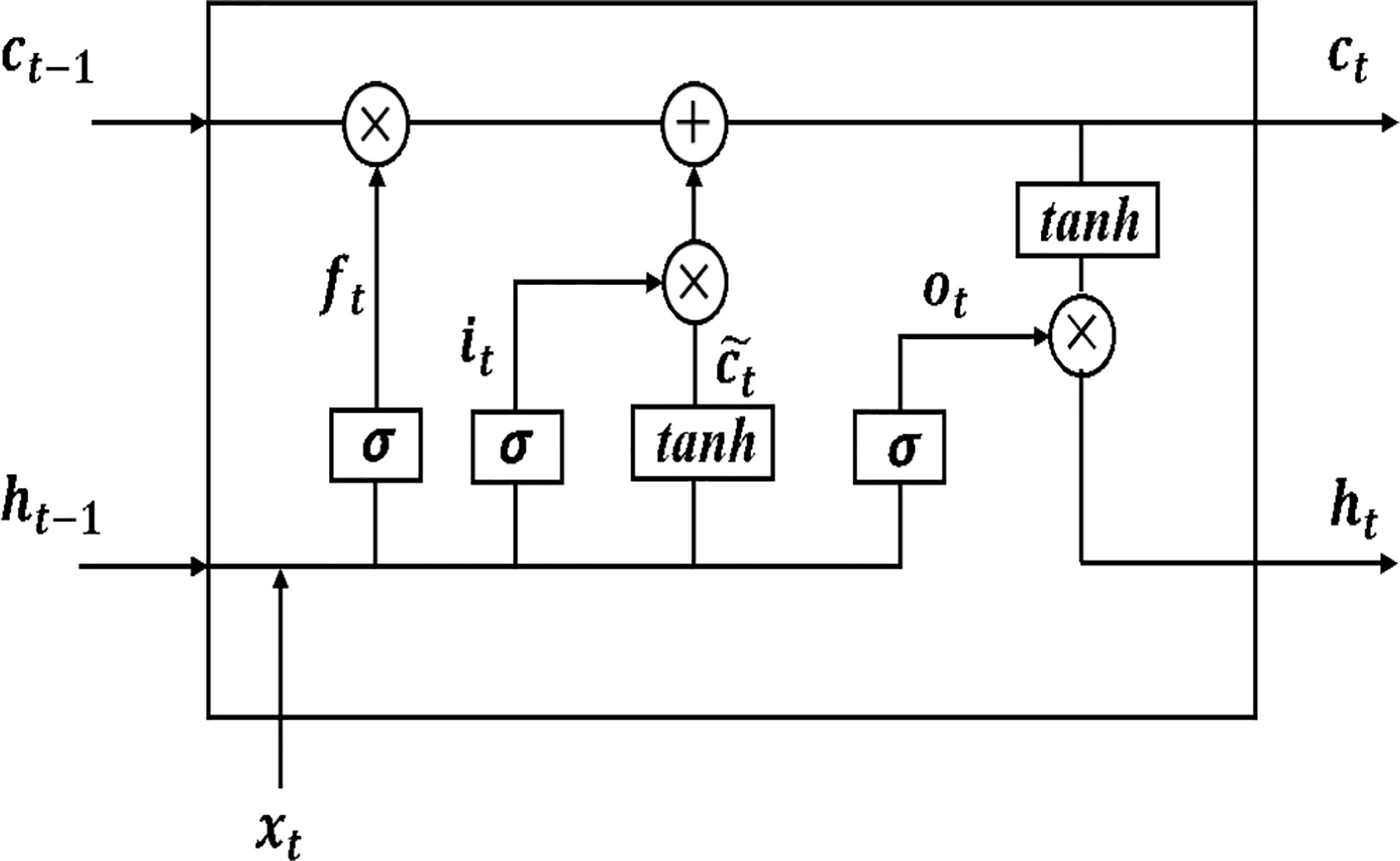
Figure 2 Internal structure of LSTM hidden layer.
and ht-1 are jointly delivered to the tanh function to create a new candidate cell state ct for the current moment, which is followed by the LSTM layer back to update the cell state ct for the current moment. The forgetting gate ftis used to control which information in the previous moment’s cell state ct-1 needs to be discarded, and then the input gate it is used to determine which information in the current moment’s candidate state ctwill be retained in the new cell state, respectively, using the product calculation. Finally, the product of the two is summed to obtain the cell state ct at the current moment. output gate ot controls the output of the current information state, i.e., the information state ht input to the next time node, which is jointly determined by x1, ht-1, and ct.
The limitation of the LSTM application in the ocean domain is that it can only handle time-series data from a single location. It is well known that the ocean is a dynamically changing whole, and different points are temporally and spatially correlated with each other (Magdalena Matulka and Redondo, 2010). Although, researchers can divide the complete ocean into multiple points and use LSTM to process them one by one. However, this approach ignores the regional characteristics of different oceans and the interactions between neighboring points of the same ocean. To address this problem. Shi et al. (2015) improved the LSTM and firstly proposed the Convolutional LSTM Network (ConvLSTM). He and his team use ConvLSTM for rainfall forecasting. They have collected many radar plots which give the distribution of clouds in a given region. Moreover, these maps are changing along the time axis. So with the past timeline and cloud cover maps, it is possible to predict where the clouds should go at future points in time, weather changes, and the chances of future rainfall in an area. Using traditional LSTM models leads to the loss of geolocation information in the cloud cover map, and therefore it is difficult to predict where the clouds will move. The contribution of the original paper is to add the convolution operation that can extract spatial features to the LSTM network that can extract temporal features and propose the architecture of ConvLSTM. ConvLSTM inherits the advantages of traditional LSTM and makes it well suited for Spatio-temporal data due to its internal convolutional structure. The computation of the ConvLSTM layer can be expressed as follows.
where * is convolution operator.
The most important feature of the ConvLSTM algorithm is that it replaces the matrix multiplication in the LSTM with convolution operations. However, its essence is still the same as LSTM, using the previous layer’s output as the input of the next layer. The difference is that with the addition of the convolution operation, the temporal relationships can be obtained, and the spatial features can be extracted like the convolution layer. In this way, Spatio-temporal features can be obtained. Regional wave height forecasting is a typical Spatio-temporal problem. Therefore, the proposed model uses the ConvLSTM algorithm.
For the wind wave prediction problem with high spatial and temporal resolution, we would like the proposed model to make longer time predictions. However, if we perform multi-step prediction directly, the error of the results may be unstable. Therefore, the proposed model adopted a different approach from most current forecasting methods that directly establish correlations between specific future moments and historical data. Instead, this study used a more appropriate forecasting strategy to improve the long-term predictive capability of the model. According to previous studies, the Rolling Mechanism (RM) is more suitable for dealing with high-frequency and long-time forecasts (Akay and Atak, 2007; Kumar and Jain, 2010).
The main idea of the RM method is to use the obtained forecast data as the latest data and add it to the future forecast. Figure 3 shows the process of forecasting. The small boxes represent the data for each moment. The numbers in the small boxes represent the moments of the data, and the large boxes represent the historical data used for each forecast (time window), which is of length N. Our forecast is a single-step forecast. First, we use the historical data from T-N to the moment T
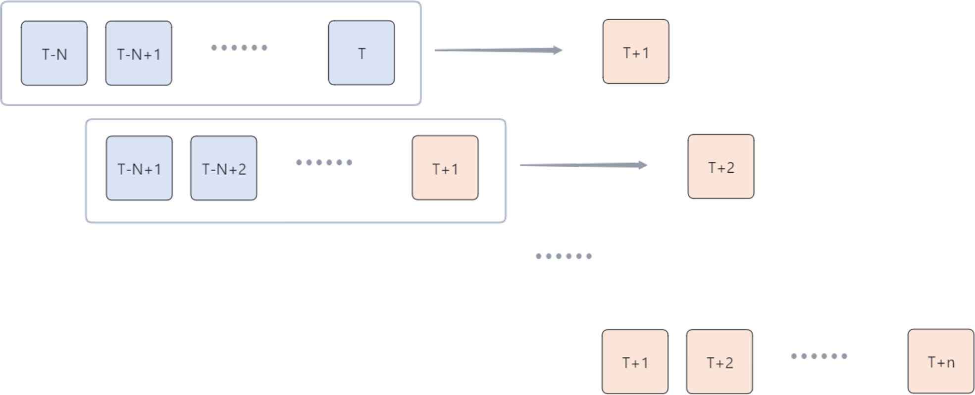
Figure 3 The prediction method integrated with RM.
to forecast the data for the future moment T+1. Immediately after that, the time window is shifted down by one step. We treat the data just obtained for T+N as known data and use the N data from T-N+1 to T+1 to forecast the data at the moment T+2, repeating the above process n times. We then get the data from T+1 to T+n moments. In this way, the prediction process of using historical data continuously to predict the next n moments is completed.
It is worth noting that the standard convolution operations in deep learning algorithms such as CNN and ConvLSTM can only act on standard rectangular areas. In our study, the study area is not a pure sea area, but a land-sea combined area, including Hainan Island and parts of the eastern Indo-China Peninsula. Due to the existence of land points, the error calculated during model training will be affected by these land points, thus affecting the effectiveness of the model. This is not what we expected. To solve this problem, we propose the Mask method described below. “Mask” is an idea in deep learning. In simple terms, it is equivalent to masking or selecting some specific elements by putting a mask over the original tensor. This study proposes the Mask method by combining the “Mask” idea.
A brief description of the Mask method is given in Figure 4. This study generates a matrix of size equal to the input data so that the points in the matrix can correspond to the points in the input data one by one. It will be referred to as the Mask matrix. The antique-white part in Figure 4 represents the land area, and we set the value of the Mask matrix corresponding to this area to 0 and the value of the Mask matrix for the ocean part represented by the blue part to 1. It is worth noting that, in practice, the land-sea distribution of the study area is much more complicated than in Figure 4. But because of the specificity of the right-angle grid data. We can still build the corresponding Mask matrix according to the idea in Figure 4. During the model’s training, the model determines the direction of the subsequent gradient descent by calculating the average error between the results and the labels. To implement our Mask method, we rewrite the loss function for network training according to Eqs.11 and 12 during network training.
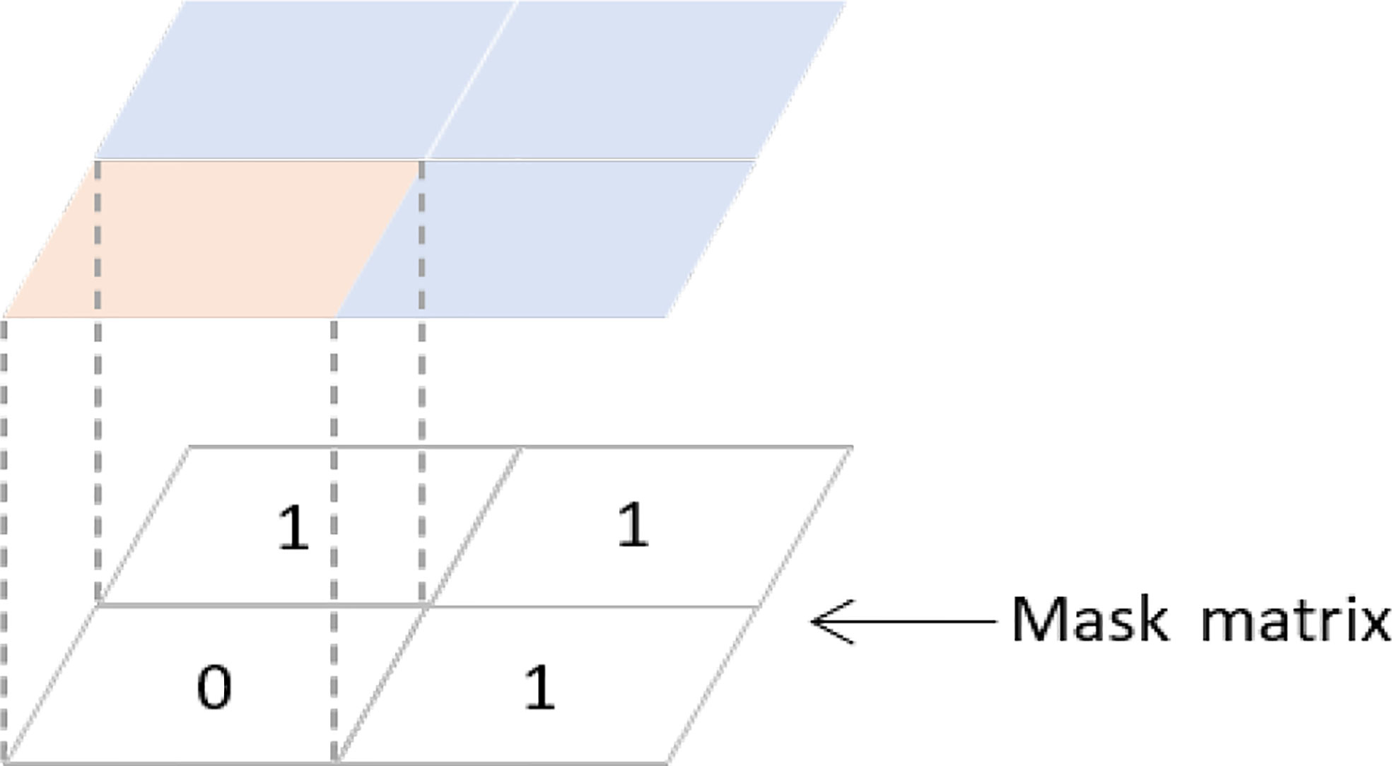
Figure 4 Idea of Mask method. The antique-white areas represent land areas and the blue areas represent ocean areas.
where U denotes the ensemble of points in the study region, Φlanddenotes points in the land region, and Φocean denotes points in the ocean region. X(t) denotes the output matrix of the prediction at this time. Yt denotes the corresponding factual matrix, and N is the number of points in the ocean area.
In this way, during the training process of the network, the result X(t) of each prediction is subtracted from the control value Yt and then dotted multiplied with the Mask matrix. Since the result is dot multiplied by Mask, and the value of the land part in the Mask matrix is zero, the error of the corresponding land part in the error matrix will also be zero. Therefore, the network only considers the error value of the ocean part in the loss value calculated in each iteration. In this way, the influence of the land region on our experiments is eliminated.
The wind and wind wave data used in this study have a spatial resolution of 1/40°*1/40° and a temporal resolution of 1 hour. Such high spatial and temporal resolution data means that the degree and speed of sea state variability are much more significant than other slightly lower resolution data. It increases the difficulty of forecasting. As mentioned earlier, there is a strong correlation between wind and wind waves in physical oceanography. If we want to exploit this correlation, we need to have both wind speed and significant wave height as inputs to the model and to have the two dependent on each other. So we need a multi-input network structure to capture this physical correlation and the subtle sea state variations. In this study, we combine the Mask method with ConvLSTM and change the number of input channels of the model to dual channels. It enables the model to meet our needs. The structure of the model proposed in this study is given in Figure 5.
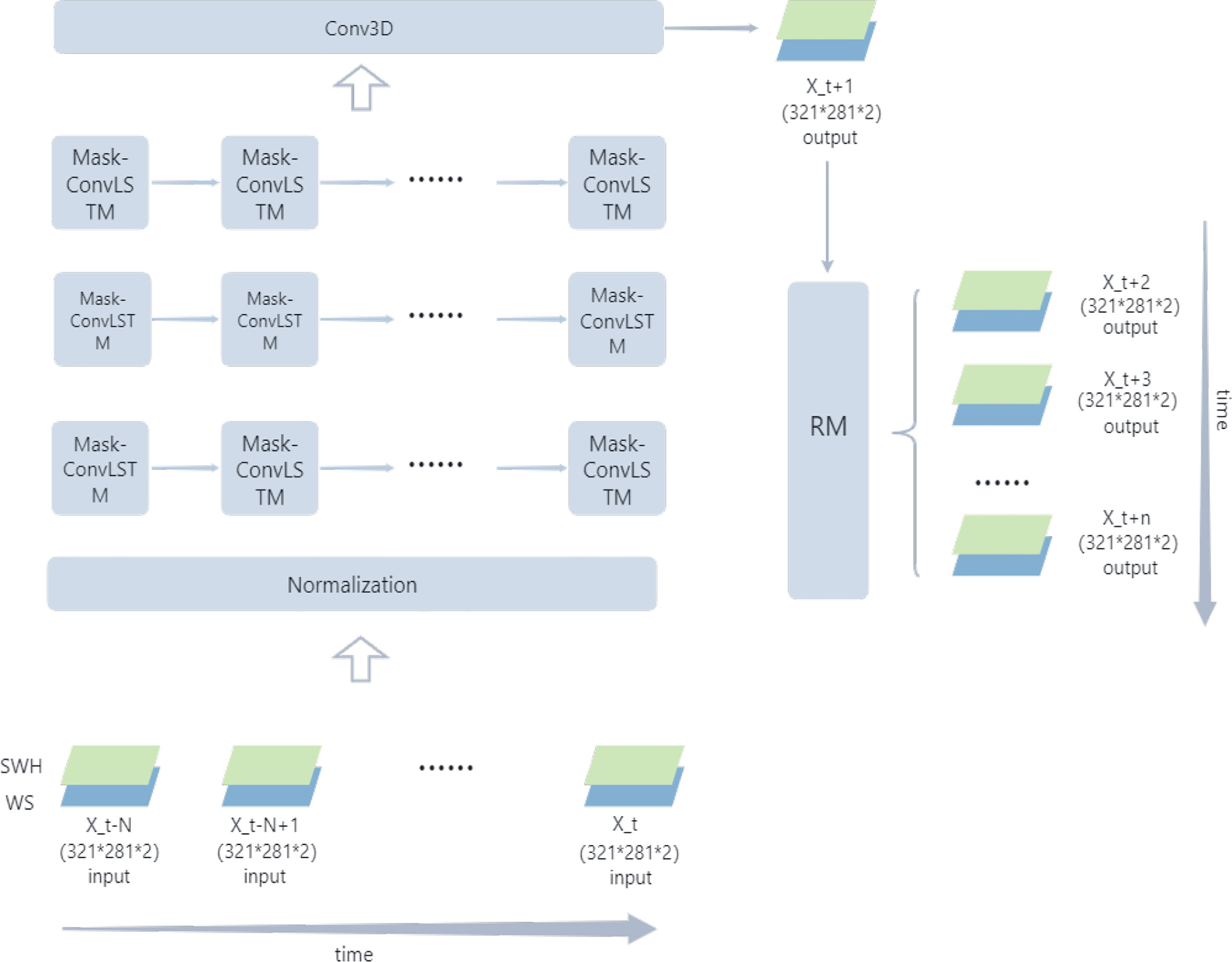
Figure 5 Architecture of the proposed model.
The input data for the model are Xt-N to Xt. Each input data consists of the wind speed (blue quadrilateral in Figure 5) and significant wave height data (green quadrilateral in Figure 5) at that moment. The data N is the length of the time window we choose. The size of these input data is (321*281) and after combining them into dual-channel data, each input X has a dimension of (321*281*2). These input data enter the regularization layer for regularization and are then fed to the three Mask-ConvLSTM layers. Between each Mask-ConvLSTM layer, model use relu as the activation function. During the model training process, the network then learns the Spatio-temporal correlation of the input data and the physical correlation between SWH and WS. Then, the size of the output data that we need to obtain is controlled by the convolution layer(Conv3D). In this way, we obtain the predicted data at Xt-N moments and then add the obtained predicted data at Xt+N moments to the RM module to achieve rolling forecasts.
In order to evaluate our model reasonably, this study selected a variety of evaluation metrics commonly used to evaluate the significant wave height prediction problem, including Root Mean Square Error (RMSE), Scatter Index (SI), and R Square (R²). In this, the SI can measure the percentage of RMSE relative to the average actual value. However, due to the specificity of the study sea area, we make some modifications to these standard evaluation metrics to match our problem. We combine the indicator RMSE,SI with our Mask method to make it possible to focus only on the error situation in the marine area. It ensures no disturbances from the terrestrial values in the area and that there are no erroneous undercounts due to incorrect, missing point counts. The mathematical equation for these evaluation indicators is as follows:
where X represents the predicted value, Y represents the corresponding value, and N is the number of points in the taken region.
The effect experiments are based on the significant wave height and wind speed data for 2018-01 to 2019-12 mentioned in Section 2. In order to test the performance of the model, this study conducted multiple sets of controlled experiments. The forecast tests were conducted in the validation set that did not participate in the training.
In order to verify the superiority of the proposed model for the high-resolution significant wave height prediction problem, this study compares several published significant wave height prediction methods. The compared methods include the traditional machine learning methods RF (Callens et al., 2020) and SVM (Berbić et al., 2017)mentioned in Section 1 and the LSTM (Fan et al., 2020), GRU (Meng et al., 2021) algorithms in deep learning. Five sets of experiments, including the model proposed in this study, used the same training data, and their performance is shown in Figure 6.
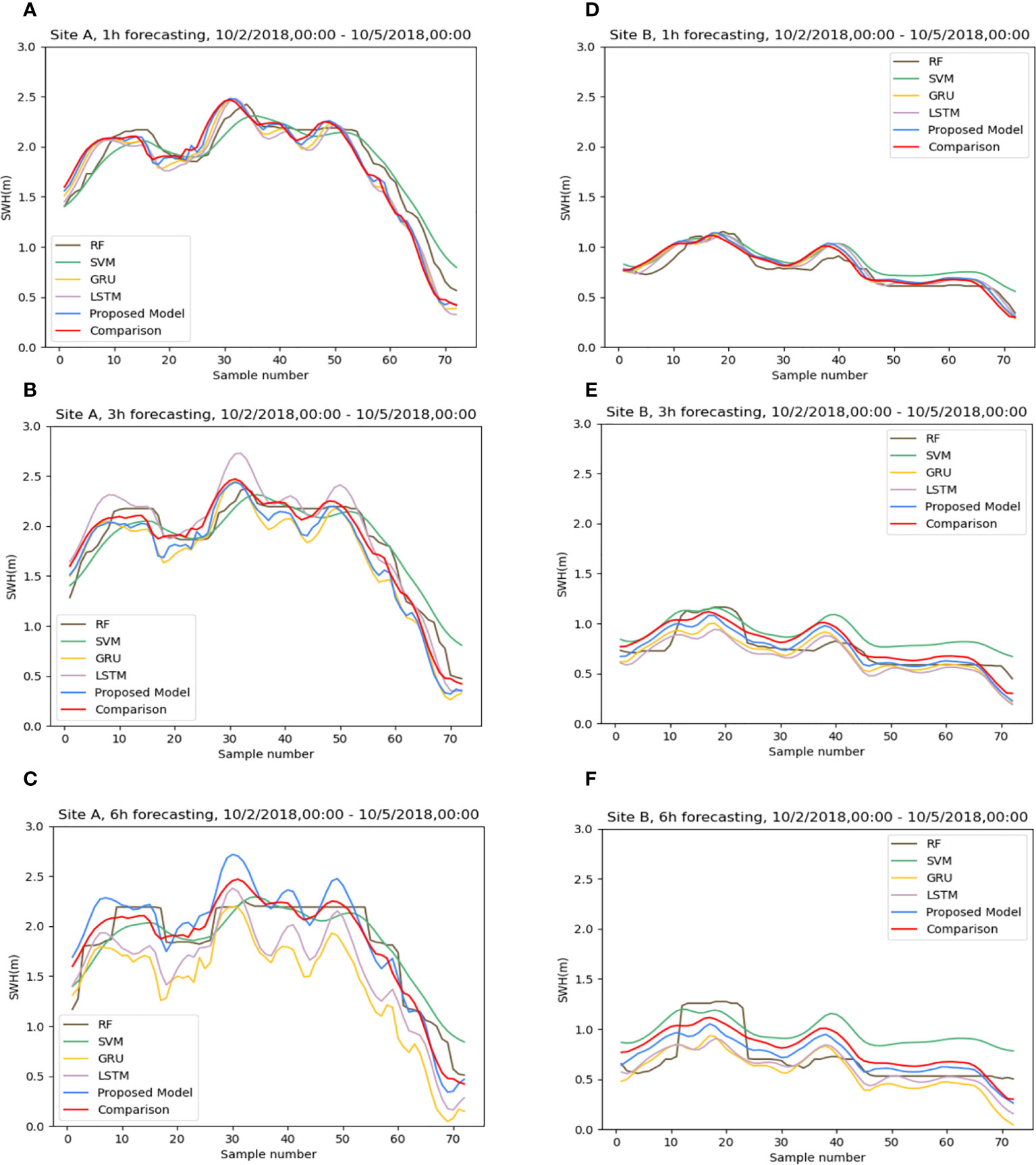
Figure 6 The differences in prediction effects of different algorithms at sites (A, B): (A, D) 1h, (B, E) 3h, (C, F) 6h. Sample number indicates the time sample number.
Firstly, this study conducted effect experiments for three different forecast lengths of 1 hour, 3 hours, and 6 hours. To more visually show the comparison of the effects between different methods, we chose two sites, siteA(17°N, 110°E) and siteB(19°N,108°E)(shown in Figure 2), to conduct our experiments. Figures 6A, D) show that at a forecast length of 1-h, there is little difference between the predicted and comparison values of the five methods. When the time grows to 3-h, the results of the RF methods show significant differences from the comparison values, especially in the case of low wind waves (Figure 6E). Although the SVM algorithm can predict the trend of data variation, the difference in values is significant. When it comes to 6-h, the RF and SVM methods have completely lost their forecasting ability. The effect of the three groups of deep learning algorithms also appears to be very different. Although LSTM, GRU, and ConvLSTM all capture the change in significant wave height, ConvLSTM has more accurate numerical magnitude predictions than the other two.
To avoid the effect of chance, we performed the above experiments for all points in the sea area and averaged the results of the comparisons, which are shown in Figures 7, 8. Figure 7A shows the variation of RMSE for the five groups of algorithms. It can be seen that the RMSE of the SVM method has reached about 0.18 at a prediction time of 1 hour. We can also visualize it in Figure 8B. The SVM algorithm lost effectiveness when the predicted large wave height was below 0.5 m. The remaining groups of algorithms do not differ much. The prediction effectiveness of the conventional machine method decays severely with time. Especially for smaller apparent wave heights, both SVM and RF show different degrees of inaccuracy. The RMSE of the SVM algorithm reaches about 0.3 for 3 hours and even 0.7 for 6-hour forecasts, while the RMSE of RF also reaches about 0.6. Two groups of deep learning methods, LSTM and GRU, have acceptable performance in the early stage (Figure 8A, C. However, the error after 6 hours is also much higher than that of the ConvLSTM method, with the RMSE increasing to more than 0.4 and the SI reaching 0.2. The comparison of the SI of different experimental groups in Figure 7B also shows the superiority of the ConvLSTM algorithm in this study. As we mentioned in Section 3, when dealing with such high spatial and temporal resolution data if only the temporal correlation of one point is considered without considering the spatial relationship of each point. It would be difficult for the model to predict the sea state changes within the sea area accurately. It may be the reason for the poor performance of the LSTM and GRU algorithms in this study.
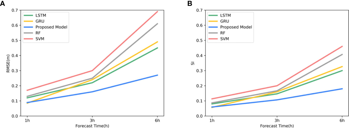
Figure 7 The difference in prediction effect of different algorithms: (A) RMSE of different algorithms varies with the forecast time, and (B) SI of different algorithms varies with the forecast time.
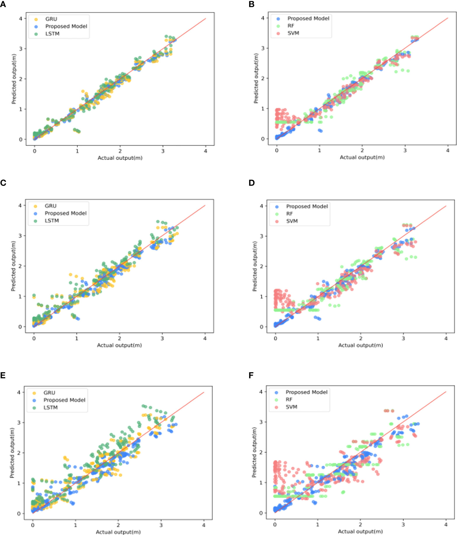
Figure 8 Scatter plots of five groups of algorithms in different forecast times: (A, B) 1 h, (C, D) 3 h, (E, F) 6 h.
In order to verify the advantages of the wind and wind waves dual-channel compared to the wave-only single channel and the effectiveness of introducing the Mask mechanism, we set up four different sets of experiments. First, a single-channel experiment using only significant wave height data for training and no Mask method (Single-channel). Second, single-channel experiments use only significant wave height data for training but with the Mask method (Single-channel & Mask). Third, experiments using significant wave height and wind speed data for training but without using the Mask method (Dual-channel). Finally, experiments using the significant wave height and wind speed for training with the Mask method (Dual-channel & Mask). It is worth mentioning that the results obtained by the dual-channel network during the prediction process are also dual-channel, containing both the prediction results of the significant wave height and the wind speed. This study aim to study the network’s prediction of the significant wave height. Therefore, we take only the significant wave height prediction results from the dual-channel network forecast results when comparing different groups of experiments.
To ensure the validity of these four sets of experiments. The hyperparameters of the four sets of experiments will be set to the same set of values. We randomly selected a period of history and made a 6-hour forecast downward using each of the four models. Figure 9 shows the results of our experiments. It can be seen that the error of the dual-channel network is significantly smaller than that of the single-channel network when only the number of channels is considered, and this situation persists with increasing forecast time. It proves the advantage of the dual-channel network. With the introduction of wind speed, the network takes advantage of the physical correlation between the two to improve our forecasting results for the significant wave height. Similarly, we can see that after the Mask method is used. When the channels are the same, the Mask-RMSE in the two groups of experiments using the Mask method is smaller than in the other two groups of experiments without the Mask method. However, we noticed a particular case. Before 3-h, the error of the single-channel network with the Mask method is smaller than that of the dual-channel network without the Mask method. It may be because the Mask mechanism can dominate the error situation brought by the forecast in the short term. However, this slowly disappears as the forecast time goes on, and both sets of dual-channel experiments slowly outperform the two sets of single-channel experiments. The above findings demonstrate the superiority of the wind and wind waves dual-channel network compared to the wave single-channel network and the effectiveness of the Mask method in this experiment.
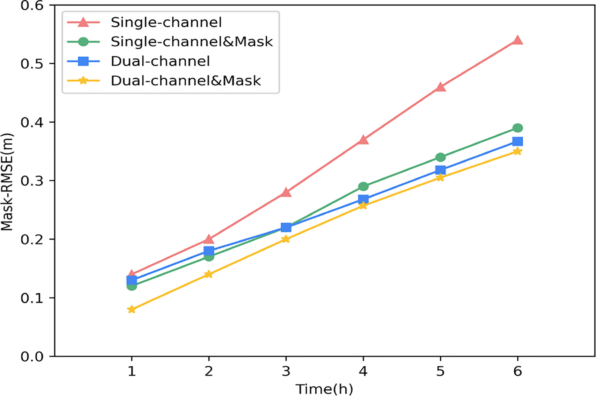
Figure 9 Mask-RMSE of the four groups varied with the forecast times.
After completing the training process of the model, we first explore the performance of the proposed model on intermediate time scales. As input data, we use 6 hours of data from 00:00-12:00 on August 28, 2019. To more visually demonstrate the ability of the proposed model to predict the high-resolution significant wave height of the study sea, we plot the results. Results and error statistics are shown in Figure 10 and Table 1.
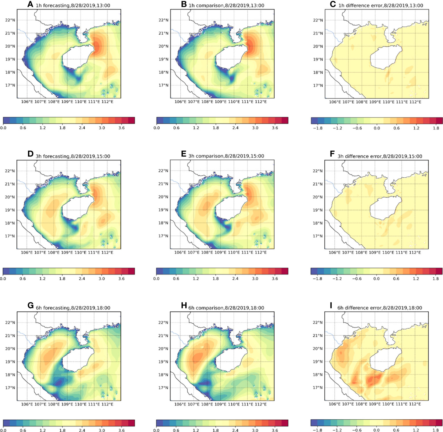
Figure 10 Comparison of forecast effect of the model under different forecast times. (A, D, G) are the predicted significant wave height effect diagrams for 1h, 3h, and 6h, respectively. (B, E, H) is the significant wave height diagram of the numerical model at the corresponding time. (C, F, I) is the difference error between forecasting and comparison.
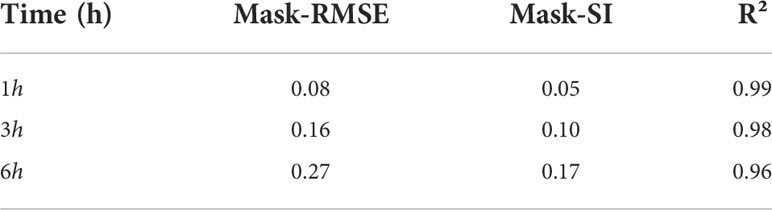
Table 1 The evaluation metrics of the model at different forecast time.
In Figure 10, the three subplots (a), (d) and (g) on the left side represent the significant wave height forecasts for 1,3,6-h, respectively. The numerical model data at the corresponding time are shown on the right side. Their evaluation indicators are shown in Table 1. We can see from Figures 10A, B that our model accurately captures the distribution of the significant wave height at 1-h with a Mask-RMSE of only 0.08 and accurately predicts the higher wind waves in the northwestern part of Hainan Island. After increasing the time to 3-h, the proposed model still has high accuracy and low error value, and the R² value can be maintained at 0.98. It also has a good prediction ability for distributing significant wave height and wave height size in the region. However, numerically, the predicted values for the western part of Hainan Island in Figure 10D are smaller than the corresponding values. When the time window comes to 6-h, although our model can still capture the significant wave height distribution in the sea, there is a significant difference in the values(Figures 10G, H). Mask-RMSE increases to 0.27. However, this value is perfectly acceptable for such high spatial and temporal resolution data. Overall, the forecasting effect of our model is excellent.
The model we use is a dual-channel network. In the prediction process, both SWH and WS channels generate errors. Because the network considers the characteristic correspondence between wind and wind waves, if the error in one channel is too large, it will also decrease the prediction of the other channel. In order to study the variation of the error of the two channels with the forecast time during the forecast, we extended the forecast time to 12-h in Section.4.3 and analyzed the error sources.
For the experimental results in Section.4.3, we analyze the error variance of the two channels in the prediction process separately. The yellow line in Figure 11 shows the trend of the prediction error of WS over time, and the blue line shows the trend of the error of SWH. It can be seen that the Mask-RMSE of both channels increases with the prediction time due to the rolling mechanism. However, on the way up, the blue line shows a steady upward trend over time, while the yellow line shows a strong upward trend, especially after 6 hours. It shows that the predictive validity of the WS channel drops significantly after 6 hours. The correlation between the two channels is considered in the model prediction process. The sharp increase in the error of the WS channel will directly lead to an increase in the error of the SWH channel, increasing the total error of the prediction results. We pioneered a new mechanism called Replace and added the Replace mechanism to the RM process to solve this problem.

Figure 11 The Mask-RMSE of significant wave height and wind speed changes with increasing forecast time.
The core idea of the Replace mechanism is to replace the predicted wind speed values of the wind speed channel in the network with the wind speed of the numerical model. As shown in Figure 12, the model is run to get the forecast output Xt+1, and the RM mechanism uses the obtained Xt+1 to continue the rolling forecast to get the output results for the next n-1 moments. The black dashed box in Figure 12 explains the specific steps of the Replace mechanism. As we mentioned before, the forecast results of each step of the model include forecast SWH and forecast WS. However, the error of WS increases sharply during the rolling forecast process (Figure 11), leading to an increase in the error of SWH associated with it. Suppose we can solve the problem of a sharp increase of WS in this process. Then the forecast results will be improved. To solve this problem, we perform the following operation for each model and RM mechanism forecast result Xt+m: replace the WS obtained from the network forecast with the WS of the numerical model to form a new Xt+m consisting of the numerical model WS and the network forecast SWH (red dashed box in Figure 12). This data is used to replace the original Xt+m for RM processing.
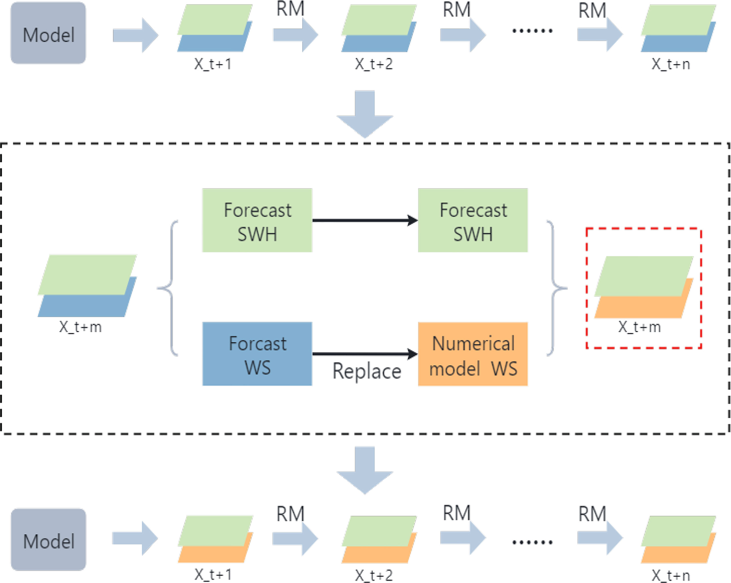
Figure 12 The idea of Replace Mechanism. The black dotted box represents the core steps of the RM mechanism, and the red box represents the data obtained through the RM mechanism.
To verify the effectiveness of the Replace mechanism, we conducted a set of controlled experiments. The error profiles of SWH before and after adopting the Replace mechanism are shown in Figure 13. The yellow line is the error plot of SWH after adopting the Replace mechanism, and the blue line is the forecast error without the Replace mechanism. It can be seen that the adoption of the Replace mechanism significantly reduces the overall forecast error, especially in the medium and long time scales. Compared to the previous one, the Mask-RMSE is even reduced by up to 50%.
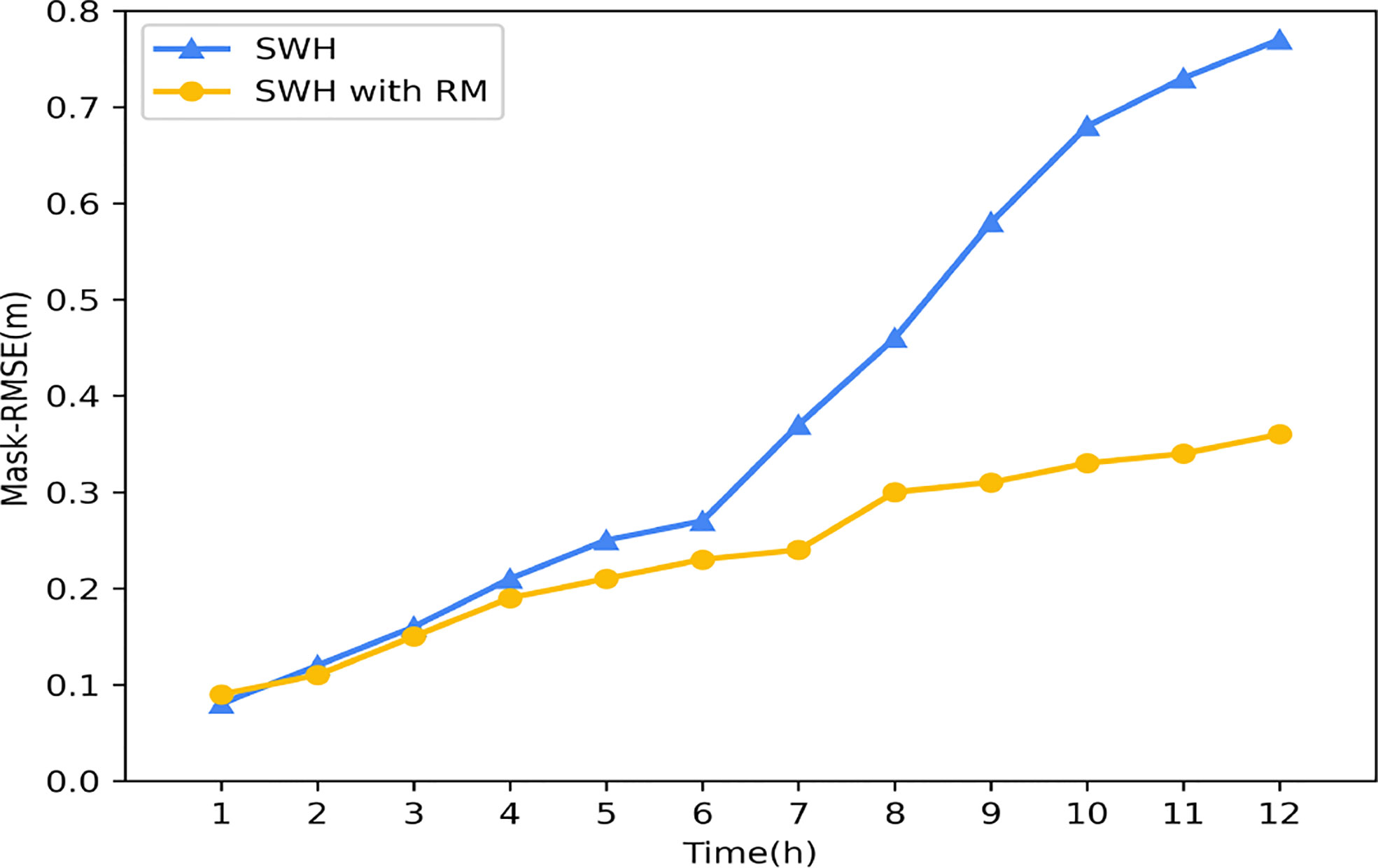
Figure 13 Comparison diagram of Mask-RMSE changes of the model before and after using the RM mechanism.
In previous deep learning wave height forecasting studies. Within the margin of error, the effective forecast duration obtained using hourly data was typically limited to 6-12 hours. If the data resolution is increased, this time will be further shortened. To investigate whether the proposed model can make predictions on long time series after using the Replace mechanism, we set up two sets of experiments. One group had Replace mechanism, and the other group had no Replace mechanism. We adjusted the timestep to 12 and retrained the model using previous data from each set of experiments. The results of the two experiments are shown in Figure 14, where (a) is the numerical model data, (b) is the prediction result of the model with the Replace mechanism, and (c) is the prediction result of the model without the Replace mechanism.
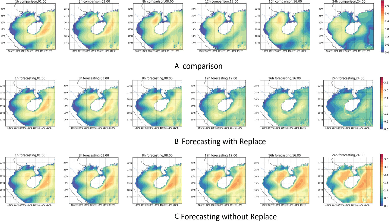
Figure 14 24-hour forecast results of significant wave height. (A) is the significant wave height diagram of the numerical model. (B) is the predicted significant wave height diagram after Replace mechanism is adopted in the model. (C) is the predicted significant wave height diagram without Replace mechanism.
We predicted the significant wave height for the next 24-hour using the data from 12:00-24:00 on August 2, 2019. The variation of each indicator with time is shown in Table 2. It can be seen that the two sets of experiments still maintain good performance at 1-hour and 3-hour (Figures 14B, C). The significant wave height and the distribution of wind waves in the sea still have a good forecasting effect. When the time reached 8-hour, the effects of the two groups of experiments began to show more apparent differences. The network without the Replace mechanism has a higher prediction of the significant wave height in the eastern part of Hainan Island. In contrast, the network with the Replace mechanism can still predict the change of the significant wave height in the sea more accurately, but the distribution has slightly deviated. When we increase the prediction scale to 12-hour, it can be seen that the model without the Replace mechanism has a significant prediction error for the change of significant wave height in the sea, and R² drops to 0.75, basically losing the accuracy of the forecast. However, the model with the replacement mechanism still has good forecasting ability, with a Mask-RMSE of 0.29. Although there are some regions where the significant wave height values are under-predicted, the overall distribution can still be predicted more accurately. When the prediction scale is expanded to 16-hour, the model without the replacement mechanism has lost its predictive power, with R² dropping to 0.62. The model with the replacement mechanism also shows a decrease in accuracy. Although the high wind and wave area near Hainan Island can be predicted, the magnitude of the significant wave height obtained from the prediction has been significantly different, with R-squared dropping to 0.78. When the time reaches 24-hour, the model without the replacement mechanism already shows confusion in the forecasts. The forecasts obtained from the predictions have little to no relationship with the contrasting values (Figure 14A). Although the model with the replacement mechanism can predict the distribution of significant wave heights in the sea area, the prediction of the magnitude of significant wave heights in the whole sea area also shows a more noticeable difference, and the R-squared drops to 0.69. Through the above experiments, we can see that: the Replace mechanism is very effective in improving the forecasts of the dual-channel network. In particular, it can effectively reduce the forecast error in a more extended time range. With the Replace mechanism, the long-time forecasting capability of the network is substantially improved, and the significant wave height at high spatial and temporal frequencies within 24 hours can be predicted more accurately.
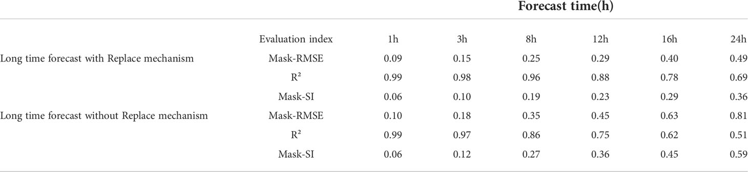
Table 2 The Evaluation index of the two model at different forecast time.
In order to verify the stability of the model’s forecasting ability, this study selected the data of SiteA and SiteB for the whole of October 2018, with a total of 744 samples. Moreover, forecast tests with different lengths were conducted using these data, and the results are shown in Figure 15. The red line in Figure 15 represent the comparison values. The yellow line represents the ERA5 reanalysis data. The blue line represents the forecast values of the model. It can be seen that the model has an excellent forecasting effect within 6-h. Both the magnitude and the trend of the values differ very little from the comparison values. When the time comes to 12-h, the model can predict the trend of the significant wave height. However, the values are not stable. When the time comes to 24-h, The model can predict the primary trend, but the values are much different in some cases. It may be because our forecasts are regional, focusing on the trend of the significant wave height within the whole region rather than the significant wave height at a single point. In addition, the insufficient amount of data in this study, which only used two years of data, might be another reason.
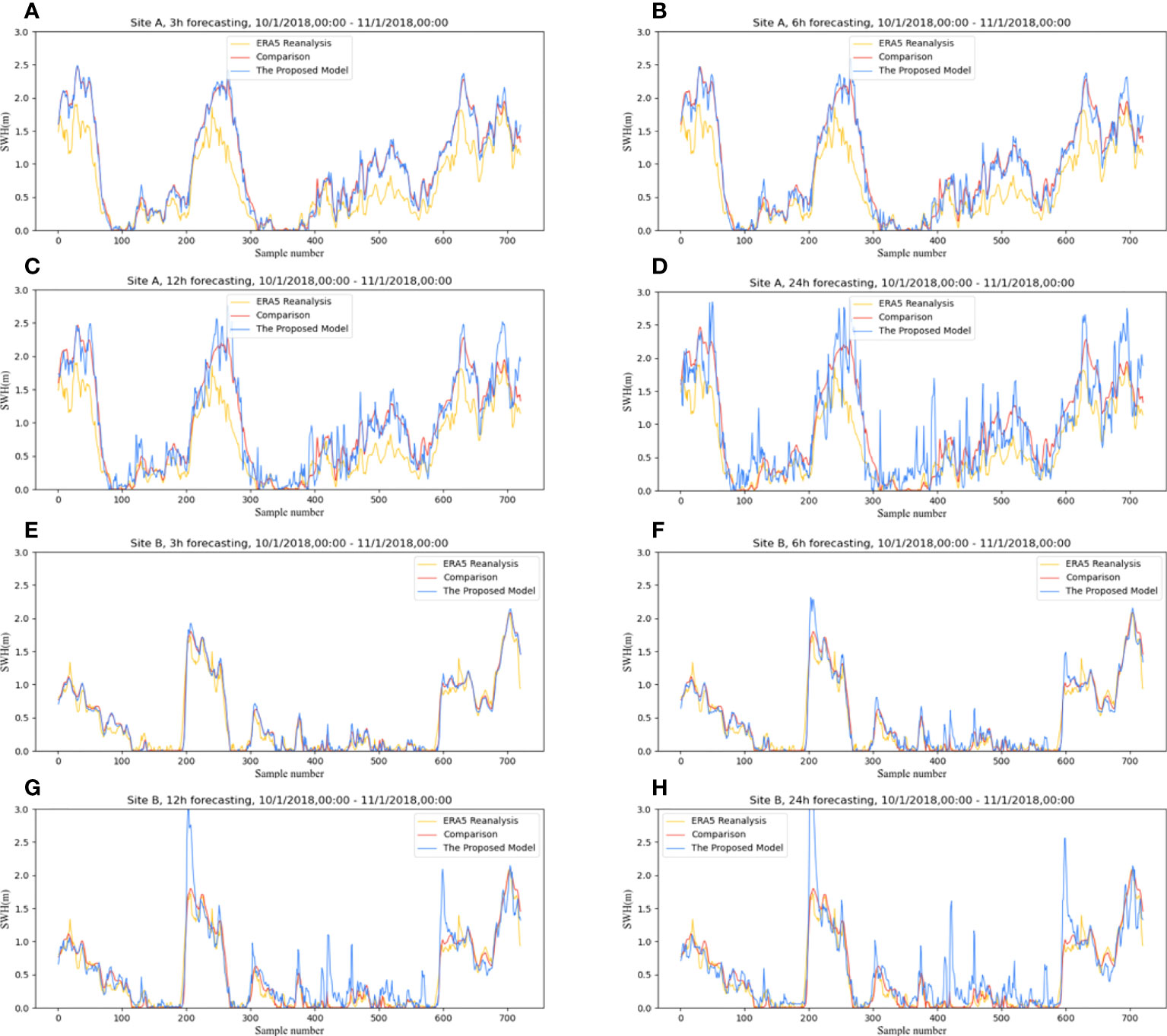
Figure 15 24-hour prediction results of significant wave heights for SiteA and SiteB. (A–D) respectively represent the 3h, 6h, 12h and 24h forecast results of SiteA, and (E–H) respectively represent the 3h, 6h, 12h and 24h forecast results of SiteB.
The main work of this research is to combine the laws of physical oceanography and use the deep learning method to predict the significant wave height of the entire Beibu Gulf with high spatial and temporal resolution. This study uses a modified ConvLSTM network to explore the Spatio-temporal correlation of historical data and the physical correlation between different marine elements. By comparing with other methods, we show the advantages of the proposed model in dealing with Spatio-temporal data. By introducing a two-dimensional wind speed field, the significant wave height prediction capability of the network is greatly improved. At the same time, this study proposes a Mask method to solve the problem of wave height prediction in sea areas with land areas. This study uses high-resolution wind speed and significant wave height data from 2018 to 2019 to conduct forecast experiments on different forecast time scales. The validity of the model is demonstrated by comparison with the numerical model. The R-squared for the 6-hour forecast reached 0.96. We analyze the error generation during the prediction process and propose an alternative mechanism to alleviate the error diffusion problem of the proposed model and prolong the effective prediction time of the network. The effective forecast time reaches 24 hours. Most importantly, the proposed model has practical application value. We know that numerical models predict waves with the wind as input. The method of this study can also utilize these wind data for wave forecasting and compare the results with short-term numerical models. It will significantly reduce the cost issues associated with numerical models. Typically, the time cost for a numerical model run to complete a prediction is over several hours and requires supercomputer support. In contrast, the model proposed in this study can be run on an ordinary PC, and the time needed for prediction is only a few seconds. It is worth pointing out that the present study was conducted for wind waves. The method proposed in this study may not be effective for a region where the wavesare mainly swell-dominated.
The proposed method also has specific problems. The first is that the RM mechanism leads to the accumulation of errors in the prediction process, and our proposed replacement mechanism can alleviate this problem to some extent. However, it cannot fundamentally solve this problem. Secondly, although the proposed model can learn some physical laws of wind speed and significant wave height, it does not really incorporate the dynamic process of the ocean in a sense. How to combine deep learning with the dynamic processes of the ocean is a problem we need to solve in the future. Thirdly, this study is only for the significant wave height, but there are other elements such as wave direction and period. If possible, we will follow up on these elements as well. Finally, we will open up the high spatial and temporal resolution data used in this work. These data will beof great help for subsequent studies.
The datasets presented in this study can be found in online repositories. The names of the repository/repositories and accession number(s) can be found below: https://doi.org/10.5281/zenodo.6402321.
TS provided overall ideas, writing review and editing, supervision, project administration, and funding acquisition. RH provided concepts, methodology, software, manuscript writing, preparation and research. FM provides formal analysis, data processing, software, and supervision. JW provided data collation and formal analysis. WW provided data management, software. SP provided methodology, method evaluation, data management, project management, and funding acquisition. All authors contributed to the article and approved the submitted version.
Innovation fund project for graduate students of China University of Petroleum (East China) (No. 22CX04008A). Project Supported by Key Laboratory of Environmental Change and Natural Disaster of Ministry of Education, Beijing Normal University (Project No. 2022-KF-08).
Over the course of my researching and writing this paper, I would like to express my thanks to all those who have helped me. A special acknowledgement should be shown to SP, from whose lectures I benefited greatly, I am particularly indebted to SP who gave me kind encouragement and useful instruction all through my writing. Moreover, I wish to extend my thanks to the library and the electronic reading room for their providing much useful information for my thesis.
The authors declare that the research was conducted in the absence of any commercial or financial relationships that could be construed as a potential conflict of interest.
All claims expressed in this article are solely those of the authors and do not necessarily represent those of their affiliated organizations, or those of the publisher, the editors and the reviewers. Any product that may be evaluated in this article, or claim that may be made by its manufacturer, is not guaranteed or endorsed by the publisher.
Akay D., Atak M. (2007). Grey prediction with rolling mechanism for electricity demand forecasting of turkey. Energy 32, 1670–1675. doi: 10.1016/j.energy.2006.11.014
Barnett T. P. (1968). On the generation, dissipation, and prediction of ocean wind waves. J. Geophysical Res. 73, 513–529. doi: 10.1029/jb073i002p00513
Barnett T., Kenyon K. (1975). Recent advances in the study of wind waves. Rep. Prog. Phys. 38, 667. doi: 10.1088/0034-4885/38/6/001
Berbić J., Ocvirk E., Carević D., Lončar G. (2017). Application of neural networks and support vector machine for significant wave height prediction. Oceanologia 59, 331–349. doi: 10.1016/j.oceano.2017.03.007
Bolton T., Zanna L. (2019). Applications of deep learning to ocean data inference and subgrid parameterization. J. Adv. Modeling Earth Syst. 11, 376–399. doi: 10.1029/2018ms001472
Booij N., Ris R. C., Holthuijsen L. H. (1999). A third-generation wave model for coastal regions: 1. model description and validation. J. geophysical research: Oceans 104, 7649–7666. doi: 10.1029/98jc02622
Callens A., Morichon D., Abadie S., Delpey M., Liquet B. (2020). Using random forest and gradient boosting trees to improve wave forecast at a specific location. Appl. Ocean Res. 104, 102339. doi: 10.1016/j.apor.2020.102339
Cooke N., Li T., Anderson J. A. (2011). The tongking gulf through history (Philadelphia, United States: University of Pennsylvania Press).
Fan S., Xiao N., Dong S. (2020). A novel model to predict significant wave height based on long short-term memory network. Ocean Eng. 205, 107298. doi: 10.1016/j.oceaneng.2020.107298
Fu Y., Zhou X., Sun W., Tang Q. (2019). Hybrid model combining empirical mode decomposition, singular spectrum analysis, and least squares for satellite-derived sea-level anomaly prediction. Int. J. Remote Sens. 40, 7817–7829. doi: 10.1080/01431161.2019.1606959
Gao J., Chen B., Shi M. (2015). Summer circulation structure and formation mechanism in the beibu gulf. Sci. China Earth Sci. 58, 286–299. doi: 10.1007/s11430-014-4916-2
Gavrikov A., Krinitsky M., Grigorieva V. (2016). Modification of globwave satellite altimetry database for sea wave field diagnostics. Oceanology 56, 301–306. doi: 10.1134/s0001437016020065
Graves A., Schmidhuber J. (2005). Framewise phoneme classification with bidirectional lstm and other neural network architectures. Neural Networks 18, 602–610. doi: 10.1016/j.neunet.2005.06.042
Hasselmann K. (1968). “Weak-interaction theory of ocean waves,” in Basic developments in fluid dynamics (Cambridge, United States: Academic Press), 117–182. doi: 10.1016/b978-0-12-395520-3.50008-6
Hochreiter S., Bengio Y., Frasconi P., Schmidhuber J., et al. (2001). Gradient flow in recurrent nets: the difficulty of learning long-term dependencies. IEEE 2001, 237–243. doi: 10.1109/9780470544037.ch14. Dataset.
Hochreiter S., Schmidhuber J. (1997). Long short-term memory. Neural Comput. 9, 1735–1780. doi: 10.1162/neco.1997.9.8.1735
James S. C., Zhang Y., O’Donncha F. (2018). A machine learning framework to forecast wave conditions. Coast. Eng. 137, 1–10. doi: 10.1016/j.coastaleng.2018.03.004
Jönsson A., Broman B., Rahm L. (2003). Variations in the baltic sea wave fields. Ocean Eng. 30, 107–126. doi: 10.1016/s0029-8018(01)00103-2
Kamranzad B., Etemad-Shahidi A., Kazeminezhad M. (2011). Wave height forecasting in dayyer, the persian gulf. Ocean Eng. 38, 248–255. doi: 10.1016/j.oceaneng.2010.10.004
Kirby J. T. (1985). “Water wave propagation over uneven bottoms,” in Tech. rep. (Florida, United States: FLORIDA UNIV GAINESVILLE DEPT OF COASTAL AND OCEANOGRAPHIC ENGINEERING).
Koongolla J. B., Lin L., Pan Y.-F., Yang C.-P., Sun D.-R., Liu S., et al. (2020). Occurrence of microplastics in gastrointestinal tracts and gills of fish from beibu gulf, south china sea. Environ. pollut. 258, 113734. doi: 10.1016/j.envpol.2019.113734
Kumar U., Jain V. K. (2010). Time series models (grey-markov, grey model with rolling mechanism and singular spectrum analysis) to forecast energy consumption in india. Energy 35, 1709–1716. doi: 10.1016/j.energy.2009.12.021
Li S., Li Y., Peng S., Qi Z. (2021). The inter-annual variations of the significant wave height in the western north pacific and south china sea region. Climate Dynamics 56, 3065–3080. doi: 10.1007/s00382-021-05636-9
Longuet-Higgins M. (1963). The generation of capillary waves by steep gravity waves. J. Fluid Mechanics 16, 138–159. doi: 10.1017/s0022112063000641
Magdalena Matulka A., Redondo J. M. (2010). Mixing and vorticity structure in stratified oceans. in. EGU Gen. Assembly Conf. Abstracts., 424. Available at: https://ui.adsabs.harvard.edu/abs/2010EGUGA..1215573M
Meng F., Song T., Xu D., Xie P., Li Y. (2021). Forecasting tropical cyclones wave height using bidirectional gated recurrent unit. Ocean Eng. 234, 108795. doi: 10.1016/j.oceaneng.2021.108795
Meng F., Xu D., Song T. (2022). Atdnns: An adaptive time-frequency decomposition neural network-based system for tropical cyclone wave height real-time forecasting. Future Generation Comput. Syst 133, 297–306. doi: 10.1016/j.future.2022.03.029
Phillips O. M. (1957). On the generation of waves by turbulent wind. J. fluid mechanics 2, 417–445. doi: 10.1017/s0022112057000233
Shao W., Sheng Y., Li H., Shi J., Ji Q., Tan W., et al. (2018). Analysis of wave distribution simulated by wavewatch-iii model in typhoons passing beibu gulf, china. Atmosphere 9, 265. doi: 10.3390/atmos9070265
Shi X., Chen Z., Wang H., Yeung D.-Y., Wong W.-K., Woo W.-c. (2015). Convolutional lstm network: A machine learning approach for precipitation nowcasting. Adv. Neural Inf. Process. Syst 28. doi: 10.48550/arXiv.1506.04214
Song T., Jiang J., Li W., Xu D. (2020). A deep learning method with merged lstm neural networks for ssha prediction. IEEE J. Selected Topics Appl. Earth Observations Remote Sens. 13, 2853–2860. doi: 10.1109/jstars.2020.2998461
Song T., Li Y., Meng F., Xie P., Xu D. (2022). A novel deep learning model by bigru with attention mechanism for tropical cyclone track prediction in the northwest pacific. J. Appl. Meteorology Climatology 61, 3–12. doi: 10.1175/jamc-d-20-0291.1
Sverdrup H. U., Munk W. H. (1947). Wind, sea and swell: Theory of relations for forecasting Vol. 601 (Washington, D.C, United States: Hydrographic Office). doi: 10.5962/bhl.title.38751
Tolman H. L., et al. (2009). User manual and system documentation of wavewatch iii tm version 3.14. Tech. note MMAB Contribution 276. Available at: https://polar.ncep.noaa.gov/mmab/papers/tn276/MMAB_276.pdf
Van Aartrijk M. L., Tagliola C. P., Adriaans P. W. (2002). Ai on the ocean: The robosail project. In ECAI (Citeseer) 133, 653–657. Available at: www.robosail.com/research/the_RoboSail_project.pdf
Wei J., Malanotte-Rizzoli P., Eltahir E. A. B., Xue P., Xu D. (2013). Coupling of a regional atmospheric model (regcm3) and a regional oceanic model (fvcom) over the maritime continent. Climate Dynamics 43, 1575–1594. doi: 10.1007/s00382-013-1986-3
Zheng K., Sun J., Guan C., Shao W. (2016). Analysis of the global swell and wind sea energy distribution using wavewatch iii. Adv. Meteorology. 2016 doi: 10.1155/2016/8419580
Keywords: wave height forecast, deep learning, high spatial and temporal resolution, new mechanism, long time prediction
Citation: Song T, Han R, Meng F, Wang J, Wei W and Peng S (2022) A significant wave height prediction method based on deep learning combining the correlation between wind and wind waves. Front. Mar. Sci. 9:983007. doi: 10.3389/fmars.2022.983007
Received: 30 June 2022; Accepted: 12 September 2022;
Published: 03 October 2022.
Edited by:
Junyu He, Zhejiang University, ChinaReviewed by:
Pushpa Dissanayake, University of Kiel, GermanyCopyright © 2022 Song, Han, Meng, Wang, Wei and Peng. This is an open-access article distributed under the terms of the Creative Commons Attribution License (CC BY). The use, distribution or reproduction in other forums is permitted, provided the original author(s) and the copyright owner(s) are credited and that the original publication in this journal is cited, in accordance with accepted academic practice. No use, distribution or reproduction is permitted which does not comply with these terms.
*Correspondence: Shiqiu Peng, c3BlbmdAc2NzaW8uYWMuY24=; Fan Meng, dmFubWVuZ0AxNjMuY29t
Disclaimer: All claims expressed in this article are solely those of the authors and do not necessarily represent those of their affiliated organizations, or those of the publisher, the editors and the reviewers. Any product that may be evaluated in this article or claim that may be made by its manufacturer is not guaranteed or endorsed by the publisher.
Research integrity at Frontiers
Learn more about the work of our research integrity team to safeguard the quality of each article we publish.