The effect of normal and abnormal eddies on the mixed layer depth in the global ocean

Mesoscale eddies are broadly distributed over the global ocean and play a significant role in modulating the spatiotemporal evolution of mixed layer depth (MLD). The presence of abnormal eddies in the ocean has been shown; however, the precise quantification of the effect of eddies on MLD, given the case of abnormal eddies, has not been carried out thus far. Differently from the previous approach to identify abnormal eddies through sea surface temperature, we therefore, proposed a method to identify abnormal eddies, using potential density based on Argo data (Array for Real-time Geostrophic Oceanography) for 15 years from 2003 to 2017. Results showed that abnormal anticyclonic eddies (AAE) and abnormal cyclonic eddies (ACE) accounted for 21.67% and 20.17% of total matching anticyclonic eddies (TAE) and the total matching cyclonic eddies (TCE), respectively, in the global ocean. The proportions of abnormal eddies were relatively higher in tropical regions but lower in regions with the boundary current and strong eddy kinetic energy. The MLD changes caused by normal and abnormal eddies were estimated combining satellite altimetry data. The normal eddies were the total matching eddies with the removal of the abnormal eddies, separately called normal anticyclonic eddies (NAE) and normal cyclonic eddies (NCE). The overall influence of NAE (NCE) was more significant on MLD deepening (uplifting) than that of TAE (TCE). Globally, NAE (NCE) changed MLD deepening (uplifting) from ~66 m (~54 m) to ~67 m (~53 m) and exhibited a more pronounced change in the Indian Ocean sector of the Southern Ocean region, from ~111 m (~94 m) to ~115 m (~92 m) in the winter. AAE (ACE), exerted a relatively weak but opposite effect on MLD deepening (uplifting). In other words, the global average MLD caused by them shoaled (deepened) from ~66 m (~54 m) to ~59 m (~59 m), and the North Pacific Ocean shoaled (deepened) from ~61 m (~47 m) to ~49 m (~57 m) in winter. Given the above results, abnormal eddies should be accounted for when the impact of ocean eddies is evaluated on the global climate system.

1. Introduction

As a boundary layer, the ocean mixed layer (ML) acts as a medium to exchange matter, energy, heat, and momentum between the atmosphere and ocean, thus playing a pivotal role in global climate change. (de Boyer Montegut et al., 2004; Carton et al., 2008). Besides, the ML is a boundary layer of the ocean that interacts with the atmosphere boundary layer. Wind forces drive ocean circulation through the ML (Chereskin and Roemmich, 1991). In areas where deep convection occurs, winter ML conditions determine the nature of deep and intermediate water masses in the interior ocean (Talley, 1999). The ocean ML also regulates biological production process, such as the mixing of phytoplankton and nutrients in and out of the euphotic zone (Chen et al., 1994; Ohlmann et al., 1996), which in turn affects the chlorophyll content. Therefore, observations of global mixed layer depth (MLD) are crucial for assessing the ocean surface layers through global climate models (Belcher et al., 2012). To quantify the spatiotemporal ML dynamics of the global and regional oceans, several algorithms have been proposed.

Traditional methods for defining the MLD fall into two broad categories, based on temperature and density (Kara et al., 2000), both of which include threshold and algorithm criteria. The threshold criterion is proposed by de Boyer Montegut et al. (2004), but Lorbacher et al. (2006) summarized uncertainties about the threshold method. In recent years, some new algorithms have emerged, such as the split merge method proposed by Thomson and Fine (2003) based on the optimal analysis of linear segments of a density profile. Their method performed similarly to the threshold method and worked in the North Atlantic, but efforts to implement it in the Southern Ocean did not yield realistic MLD results. The density algorithm, proposed by Holte and Talley (2009), to identify physical features in the profiles allow for more accurate tracking and identifying of the MLD than that of the traditional threshold method. However, because of its complexity, the algorithm is slower than the threshold and gradient methods and as with any MLD algorithm, is prone to be influenced by unusual profiles. The curvature method reported by Chu and Fan (2010) has the following characteristics: (1) the determination of MLD depends on downward profile data from the surface; (2) the procedure is objective without any initial assumptions (no iteration); and (3) no differentiations are calculated for the profile data. Temperature profiles in the western North Atlantic Ocean from November 14 to December 5, 2007, collected from two gliders (Seagliders), demonstrate the capability of this method. The algorithm is analogous to a full range of local “ventilation” depth proposed by Chen and Yu (2015). Property-adaptive, the algorithm provided a significant periodic geophysical forcing, such as the annual cycle. A significant discrepancy between their and other results is the existence of a constantly deeper MLD band in the mid-latitude oceans of both hemispheres. However, the algorithm is more complex than the others. The primary advantage of climatology of the hybrid algorithm by Holte et al. (2017) is that not only is it a more accurate method used for identifying the MLD, as shown by a quality index analysis, but also more density profiles are incorporated than before in the previous climatologies.

The oceanic eddies cover more than 40% of the global ocean surface and contain approximately 90% of the total energy of the ocean (Klein and Lapeyre, 2009; Ferrari and Wunsch, 2010). They are the drivers of the rotating motion of seawater with a scale smaller than that of the Rossby wave. The quasi-geostrophic potential vorticity equation controls them, including vortex, swirl, ring, meander, filament, and wake (Robinson, 1983). Their horizontal scales are about a few to hundreds of kilometers, spanning the mesoscale and sub-mesoscale in oceanography, and the vertical scales are about tens of meters to thousands of kilometers (penetrating ML and thermocline) (Chelton et al., 2011). The time scales of eddies are about several days to several years (Chelton et al., 2011). Oceanic eddy detection is a critical step in promoting the development of eddy science, which has been widely implemented based on various remote sensing data in recent years, such as satellite altimeters, synthetic aperture radar, and ocean buoys. The mainstream of the eddy identification method is an automatic algorithm based on sea level anomaly (SLA) grid maps, which has been proven effective (Chelton et al., 2011; Faghmous et al., 2015; Le Vu et al., 2018).

For total matching cyclonic eddies (TCE), the eddy produces an upward flow, causing a greater density inside the eddy than in the surrounding seawater, which results in a positive density anomaly. The eddy is termed as an abnormal cyclonic eddies (ACE) if the density is a negative anomaly. Similarly, for total matching anticyclonic eddies (TAE), the eddy produces a downward flow, causing a lower density inside the eddy than in the surrounding seawater, resulting in a negative density anomaly. If the density is a positive anomaly, the eddy is termed as an abnormal anticyclonic eddies (AAE). Various studied have been conducted about abnormal eddies based on the SST method. Globally, the numbers of the warm cyclonic and cold anticyclonic eddies identified via measurement instruments and deep learning models were estimated at approximately 20% by Ni et al. (2021) and 32% by Liu et al. (2021), respectively. Regionally, Sun et al. (2019) and Sun et al. (2021) separately detected abnormal eddies in the North Pacific and the South China Sea. Several studies have posed the following possible mechanisms for generating abnormal eddies based on SST: (1) Anticyclonic cold-core eddies emerge from mode water created by deep winter mixing (Martin and Richards, 2001). (2) Eddy–wind interaction-driven upwelling in anticyclones forms anticyclonic cold-core eddies (known as mode water eddy), whereas eddy–wind interaction-driven downwelling in cyclones produces cyclonic warm-core eddies (Mcgillicuddy, 2015). (3) Reinforcement with the supply of cold and fresh water results in anticyclonic cold-core eddies, and that with warm water causes cyclonic warm-core eddies (Yasuda et al., 2000; Rabinovich et al., 2002). (4) The cyclonic warm-core eddies - anticyclonic cold-core eddies are a result of caused by the baroclinic instability (Pickart et al., 2005; Kadko et al., 2008; Carton et al., 2008). (5) Instability during the decay stage, eddy-eddy interaction, and horizontal entrainment result in abnormal eddies (Sun et al., 2019).

Researches have concluded that mesoscale eddies modulate the spatiotemporal evolution of MLD (Klein et al., 1998). The vital role of the mesoscale eddies in redistributing MLD has been well established. For example, Gaube et al. (2019) analyzed how mesoscale eddies globally modulate the surface MLD and found that the magnitude of eddy-induced MLD anomalies is largest during winter in regions of large- amplitude edd ies. Similarly, as Hausmann et al. (2017) reported, the net deepening of the MLD by the eddies is expected to be greatest in the regions of large-amplitude eddies and deep winter mixing in the Indian Ocean sector of the Southern Ocean. The asymmetry that MLD anomalies are more prominent in magnitude in anticyclones than in cyclones has been observed in the Indian Ocean sector of the Southern Ocean (Hausmann et al., 2017) and the South Indian Ocean (Kouketsu et al., 2012; Gaube et al., 2013; Dufois et al., 2014). However, the role of abnormal eddies in MLD remains unclear in related literature.

The main objective of this study was two-fold: (1) to propose a new perspective to identify abnormal eddies based on the potential density and (2) to analyze the impact of normal and abnormal eddies on MLD. The dramatic improvement in state-of-the-art spatiotemporal sampling and coverage of the Argo project allowed us to obtain a unique and detailed dataset of subsurface temperature (T) and salinity (S) records. The rest of the paper is organized as follows: In the Data, we describe the three datasets (altimetry, Argo data, and MLD) used in this study. The Methodology includes the method for data-preprocessing, identification algorithm for normal and abnormal eddies, and formula for eddy-induced MLD anomalies. In Results, findings are presented in two subsections: (1) the global distribution and proportion of abnormal eddies; and (2) the spatiotemporal distribution of MLD inside eddies (including total matching, normal, and abnormal eddies) and the quantitative evaluation of the impact of eddies on MLD. Discussion contains the possible generation mechanisms of abnormal eddies and the reasons for the different effects of normal and abnormal eddies on MLD. Finally, the summary of this study is given in the Conclusions.

2. Data

2.1. Satellite altimeter data

The altimeter data used in this study are delayed-time products generated by CMEMS from a combination of TOPEX/Poseidon (T/P), ERS-1/2, Envisat missions, Jason-1, Jason-2, Jason-3, Sentinel-3A, HY-2A, Saral/AltiKa, Cryosat-2, and GFO missions (CMEMS, 2019). In order to seek a better consistency which is vital to eddy identification, it is decided to apply the CMEMS “all-satellite” merged dataset of daily mean SLA with a grid size of (1/4) ° × (1/4) °, spanning from January 2003 to December 2017. A sub-dataset is used for simultaneous analysis with Argo measurements. A comprehensive eddy dataset has been created for the global ocean, which can be found at: https://data.casearth.cn/thematic/Global_ocean_eddies?lang=zh_CN (Tian et al., 2020).

2.2. Argo float

The delayed-time Argo data (Array for Real-time Geostrophic Oceanography) from January 2003 to December 2017 were used. Argo floats are aimed at observing significant temporal (seasonal and longer) and spatial (thousands of kilometers) scale subsurface (to a depth of 2,000 m) ocean variability worldwide (Roemmich et al., 2009). The Argo project is the first global observation system for the subsurface ocean and is one of the best sources for in-situ temperature measurements (Chen et al., 2021b). Because of its unprecedented spatiotemporal sampling and coverage, the Argo project has created an enormous dataset of subsurface T and S records that can be used to study the distribution and variability in MLD. In this study, Argo profiles with T/S measurements were obtained from http://www.argo.ucsd.edu. The quality control and processing of Argo data are automatically conducted by the Argo Data Center, and only profiles flagged as “good” or “probably good” were downloaded. Additional data filtering was applied to profiles with first measurements shallower than 10 m, last measurements deeper than 1000 m, and having at least 30 valid data points within a depth range of 0–1,000m. Finally, linear interpolation with an interval of 1 m was performed for all edited high-quality profiles in the global ocean.

The vertical structure anomalies caused by eddies can comprehensively assessed through T/S data-derived density. Therefore, in this study, the potential density anomaly (PDA) was selected as the property to represent the vertical structure of eddies for abnormal eddy identification. Once the profile data were preprocessed and filtered, the potential density was estimated based on the International Thermodynamic Equation of Seawater 2010 from Argo T/S profile data, using the Gibbs Seawater Oceanographic toolbox (Mcdougall et al., 2010). Anomalies of every profile were computed by removing climatological profiles. In this study, the monthly climatological density profiles were obtained from the 3° × 3° grid resolution Argo profile.

2.3. Mixed layer depth

Several criteria have been suggested in related literature for defining MLD (de Boyer Montegut et al., 2004; Holte and Talley, 2009; Holte et al., 2017, etc.). This study used the database proposed by Holte et al. (2017), calculated with a hybrid algorithm and a standard threshold method for detecting MLD. The database is available online at http://mixedlayer.ucsd.edu and provides monthly estimates of MLD (mean, median, maximum, and standard deviation), along with associated properties (mean density, temperature, and absolute salinity). Their database uses a highly accurate method for identifying MLD, as shown by a quality index analysis. It also incorporates a greater number of density profiles than those in the previous climatologies and is publicly available. The hybrid algorithm included the density algorithm from Holte and Talley (2009) and the variable density threshold from de Boyer Montegut et al. (2004). The basic idea of the algorithm was to simulate general shape of each profile via the best-fit lines to the seasonal thermocline and ML. Next, it calculates the threshold MLD, gradient MLD, intersection of the seasonal thermocline, ML fits, and property maxima and minima. The above values were analyzed to select the final MLD estimate.

3. Methodology

3.1. Altimeter-based eddy identification

In the present analysis, a four-step scheme has been established for eddy identification based on our earlier works by Liu et al. (2016); Sun et al. (2017); Tian et al. (2020). First, the global SLA data was high-pass filtered with a Gaussian filter with a zonal radius of 10° and a meridional radius of 5° before seed points were effectively determined. Second, the global SLA fields were divided into regular blocks with a zonal spacing of 45° and a meridional spacing of 36°. Third, the SLA contours were computed using a 0.25-cm interval to extract the eddy boundaries. Lastly, all blocks were seamlessly merged into a global map, and duplicate eddies were eliminated. The relevant technical details (including models and programs) can be found in Liu et al. (2016); Sun et al. (2017), and Tian et al. (2020).

3.2. Eddy matching using the Argo data

To describe the effect of eddies on MLD, a “point-in-polygon” search was employed to confirm whether an Argo float was present inside an eddy (de Marez et al., 2019). First, we selected the eddies and Argo float on the same day, and the location of each Argo float profile was used to match the nearest eddy center in the effective eddy boundary. In the present study, the effective eddy boundary and the last closed contour of an eddy were selected as the eddy contour. Second, it was determined whether an Argo float was present inside the eddy. An Argo float was considered collocated with an eddy if it was within the size of the eddy boundary. Next, the relative radius (r) was calculated as follows:

$\begin{array}{ll}r=\frac{S}{L}& (1)\end{array}$

where S and L are the distance of Argo from the eddy center and the distance from the eddy center in the same direction to the eddy boundary, respectively. Finally, an Argo float-eddy collocation dataset was created following a global search of all Argo floats with this criterion. In this study, the total matching eddies were selected satisfying the following two criteria: (1) the lifespan was longer than or equal to 30 days and (2) the pixel was not less than 9. The numbers of profiles that were classified as TAE and TCE were 205,374 and 200,254, with a match rate of approximately 1.92% and 1.82%, respectively. Figure 1 shows the geographical distribution of the Argo profiles. In general, the Argo float samples are almost all over the global ocean but are more numerous in the Kuroshio area, the Mediterranean Sea, the Arabian Sea, and the Bay of Bengal (Figure 1A). Similarly, the number of Argo floats falling within the eddies is higher in several of the above regions (Figures 1B, C).

FIGURE 1

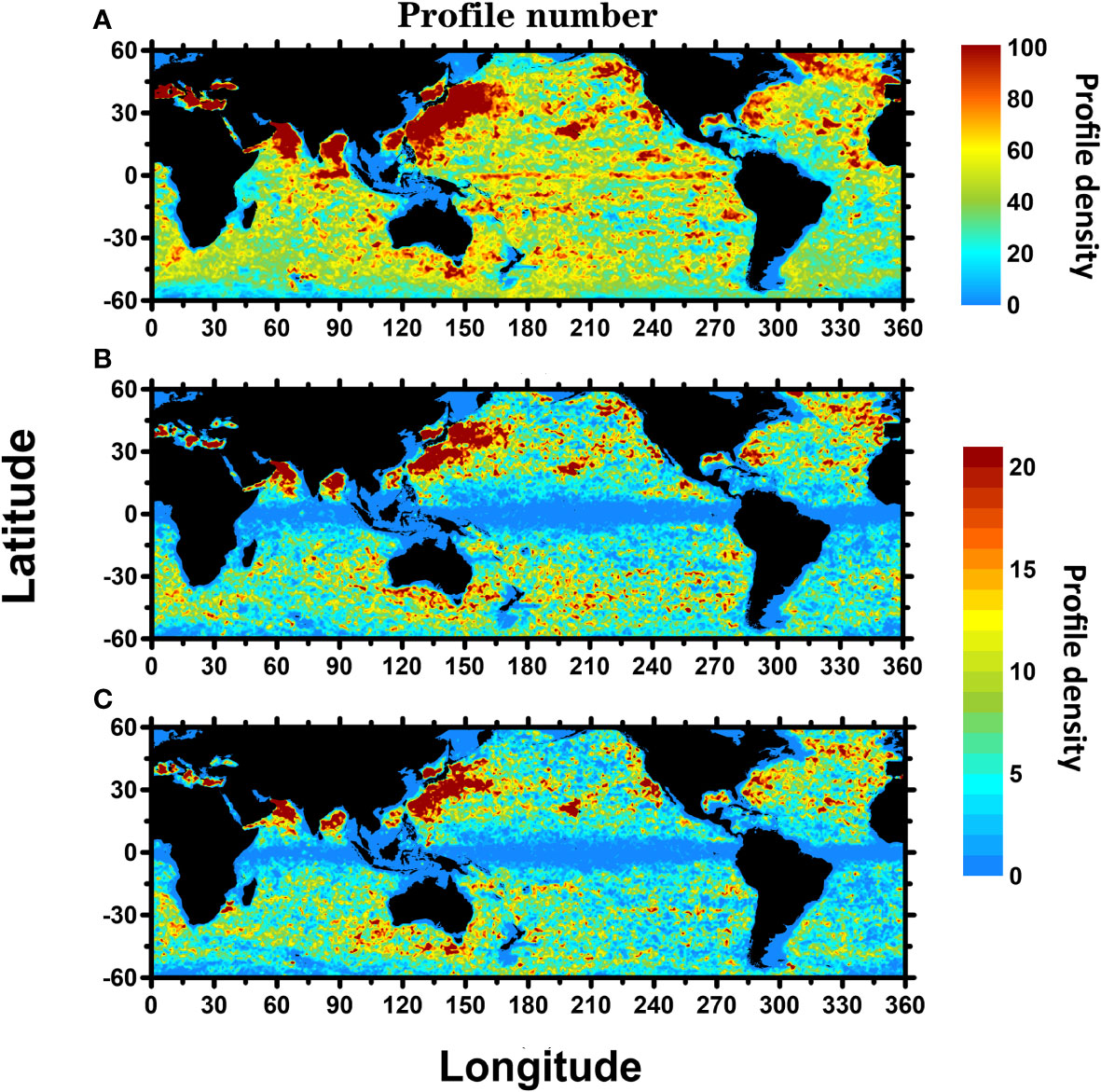
Figure 1 Global geographic distribution of Argo profiles during 2003–2017 under 1° × 1° grid. (A–C) Cumulative number of all profiles, profiles inside total matching anticyclonic eddies and total matching cyclonic eddies, respectively.

3.3. Definition of abnormal eddies

The eddies satisfying the following criteria were defined as abnormal eddies: the integral value of PDA of TAE (TCE) per unit depth in the respective eddy core depth > 0 (<0). In this study, we used the eddy core depth proposed by Chen et al. (2021a). The global distribution of eddy core depth is shown in Figure 2. In general, the abnormal eddies refer to eddies whose enclosed PDA has an opposite sign concerning their altimeter-identified polarity, as shown in Figure 3. That is, from the Argo perspective, they cannot be classified as eddies with the same polarity. In this analysis, PDA was chosen as the property to represent the vertical structure of eddies.

FIGURE 2

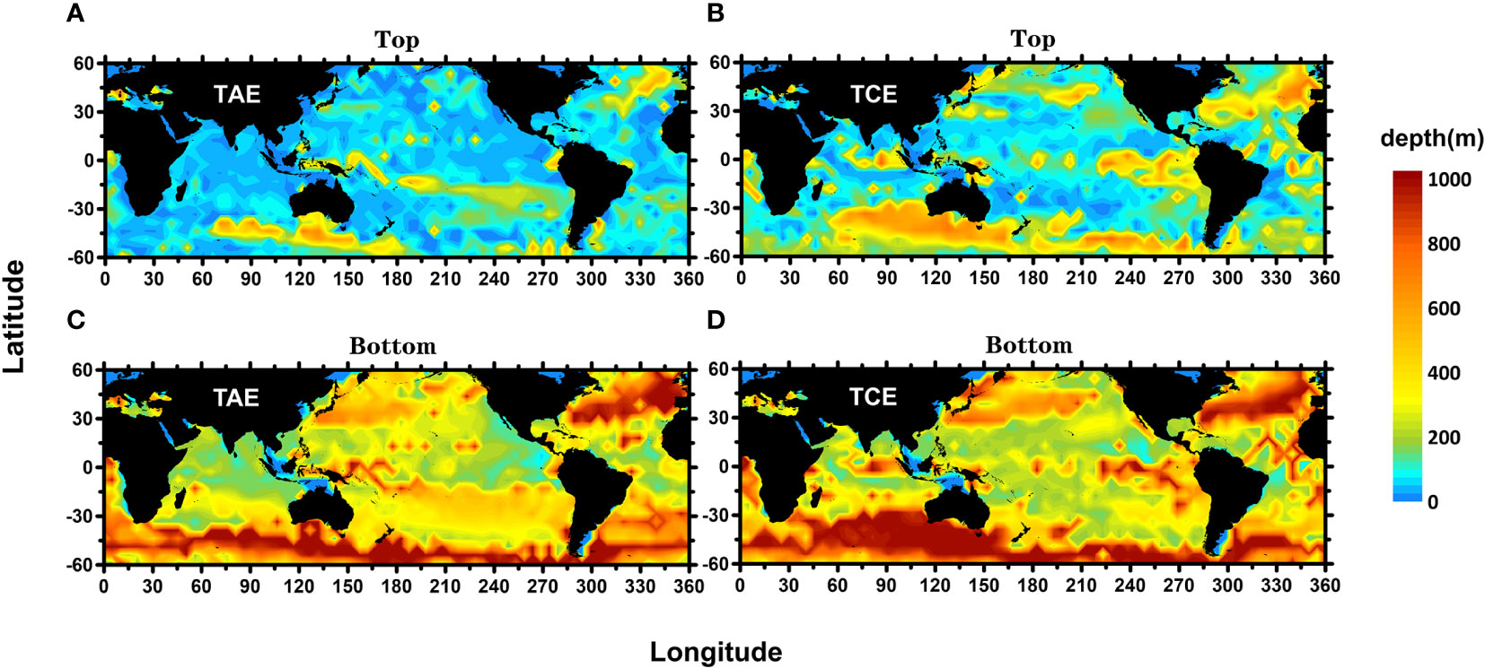
Figure 2 Global distributions of eddy core depth at 5° × 5° resolution. The (A, B) panels are the top and bottom of the eddy core depth respectively, and the (C, D) are for TAE and TCE, respectively.

FIGURE 3

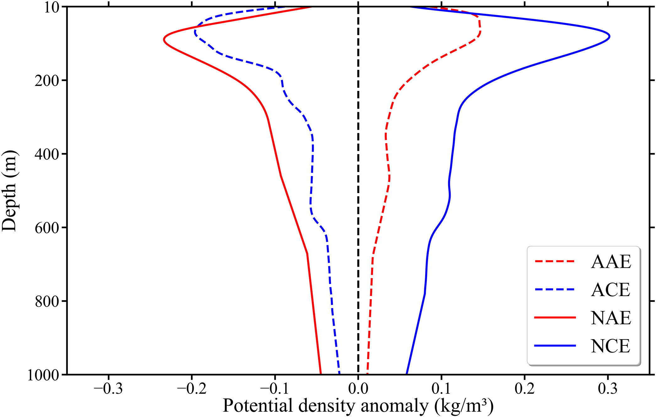
Figure 3 Globally averaged PDA vertical profiles for normal and abnormal eddies during January 1, 2003 to December 31, 2017. The solid (dashed) red line and solid (dashed) blue line represent NAE (AAE) and NCE (ACE), respectively.

3.3.1. The method for calculating PDA from Argo measurements contains the following steps:

(1) The potential density was estimated based on the T/S profile according to the International Thermodynamic Equation of seawater 2010 (TEOS-10), using the Gibbs Seawater Oceanographic toolbox (Mcdougall et al., 2010):

$\begin{array}{ll}\begin{array}{c}{\mathit{\text{ρ}}}^{\mathit{\theta }}\left({\mathit{\text{S}}}_{\mathit{\text{A}}},\mathit{\text{t}},\mathit{\text{P}},{\mathit{\text{P}}}_{\mathit{\text{r}}}\right)=\mathit{\rho }\left({\mathit{\text{S}}}_{\mathit{\text{A}}},\mathit{\text{θ}}\left[{\mathit{\text{S}}}_{\mathit{\text{A}}},\mathit{\text{t}},\mathit{\text{P}},{\mathit{\text{P}}}_{\mathit{\text{r}}}\right],{\mathit{\text{P}}}_{\mathit{\text{r}}}\right)\\ = {\mathit{\text{g}}}_{\mathit{P}}^{-\mathit{1}}\left({\mathit{\text{S}}}_{\mathit{\text{A}}},\mathit{\text{θ}}\left[{\mathit{\text{S}}}_{\mathit{\text{A}}},\mathit{\text{t}},\mathit{\text{P}},{\mathit{\text{P}}}_{\mathit{\text{r}}}\right],{\mathit{\text{P}}}_{\mathit{\text{r}}}\right)\end{array}& (2)\end{array}$

where ρ is the potential density, S_A is absolute salinity, which can be obtained through the reference salinity and sea pressure; t and θ are the in-situ temperature and potential temperature, respectively; P and P_r are the pressure and reference pressure, respectively; and g_P is the expression of Gibbs function as follows:

$\begin{array}{ll}{g}_P\left(S_A,t,P\right)= g^W\left(t,P\right)+g^S\left(S_A,t,P\right)& (3)\end{array}$

where g^W and g^S are the pure-water and saline parts of Gibbs function, respectively.

(2) Monthly climatological profiles were constructed at a spatial resolution of 3° × 3° to calculate the climatological average value of the potential density within each grid. In this study, the resolution of 3° × 3° was adopted to ensure the availability of enough data in each grid.

(3) The PDA per unit depth profile was obtained removing the collocated (space and time) climatological mean of the potential density at this depth. This process is repeated for all the individual Argo profiles in the global ocean.

3.3.2. The algorithm for defining abnormal eddies is as follows:

(1) PDA per unit depth was integrated over the eddy core depth. The integral interval was the top and bottom of the eddy core depth. We set the lower limit of integration as 10 m, neglecting the values below this depth in the calculation because the calculation of MLD started from a depth of more than 10 m. This process is described as Eq. (4).

$\begin{array}{ll}v=\underset{a}{\overset{b}{\int }}f\left(x\right)dx (10m\le a<b<1000m)& (4)\end{array}$

where a and b are the top and bottom limits of the eddy core depth, respectively. The integral of PDA and PDA at per unit depth are expressed by v and f , respectively.

(2) If v > 0 in TAE, the eddy was considered as AAE; if v < 0 in TCE, the eddy was considered as ACE.

To study the distribution of abnormal eddies, the occurrence ratio of abnormal eddies was defined thus:

$\begin{array}{ll}F(\%)=\frac{n_{abnormal}}{n_{total}}& (5)\end{array}$

where n_abnormal and n_total are the numbers of abnormal and total matching eddies, respectively.

3.4. Eddy-induced mixed layer depth

This study used MLD estimates from hydrographic profiles collected by the autonomous Argo float array (Holte et al., 2017). As the density is more stable than temperature, we preferred the density-based algorithm for MLD described by Holte and Talley (2009). If the density data were missing, we used the temperature-derived threshold-based values as the MLD estimate (de Boyer Montegut et al., 2004). Our global MLD range covered 60° S~60° N. To reflect eddy-induced MLD, anomalies of MLD (MLD^′) were calculated through the removal of the climatological MLD at a given location (x, y) and time t (Gaube et al., 2019) as follows,

$\begin{array}{ll}ML{D}^{\prime }\left(x,y,t\right)=MLD\left(x,y,t\right)-\overline{MLD}\left(x,y,m\right) & (6)\end{array}$

where $\overline{MLD}$ is the climatological MLD at location x,y (latitude and longitude), and month m . Positive MLD' was defined here as a MLD deeper than climatology. The climatological MLD is on a 3° × 3° grid.

4. Results

4.1. Detected abnormal eddies

Globally, approximately 21.67% of TAE were AAE, whereas 20.17% of TCE were ACE. Figure 4 shows the proportions of abnormal eddies in the global 3° × 3° grid. AAE and ACE occurred more frequently in tropical regions, which was consistent with the study of Chen et al. (2021a) and Ni et al. (2021). The numbers of abnormal eddies and ratios with different relative radii in the five regions (reference Gaube et al. (2019)) are shown in Table 1. The number and proportion of abnormal eddies rose with the increased relative radius. The increase in the abnormal rate from 0.3r to 0.5r was slight but considerably ranged from 0.5 r to 1 r, a 50% change.

FIGURE 4

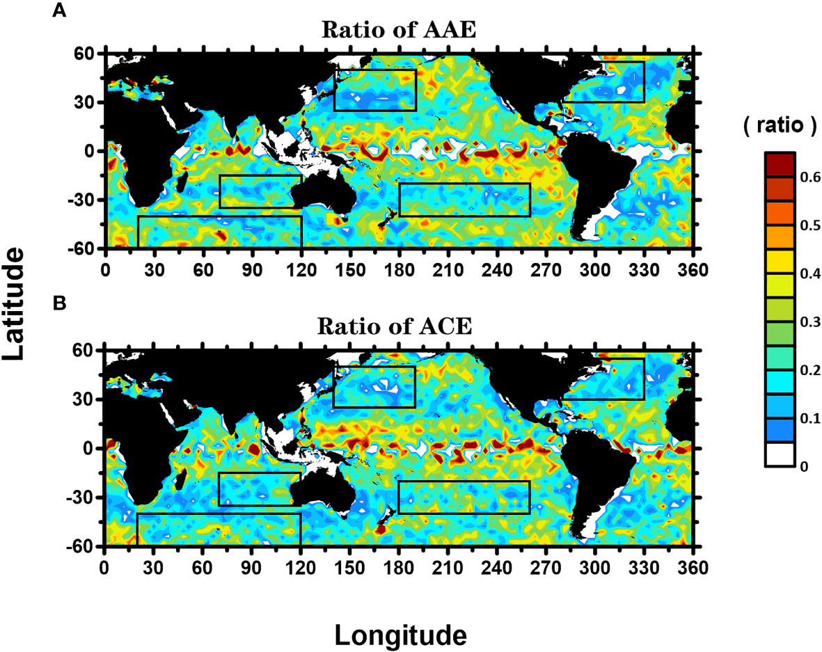
Figure 4 Proportions of abnormal eddies in global 3° × 3° grid. The ratio of the number of AAE (A) and ACE (B) to the number of TAE and TCE detected in each grid over the 15-yr period of 2003–2017. The black box indicates five areas (NA, North Atlantic Ocean 30°–55° N, 280°–330° E; NP, North Pacific Ocean 25°–50° N, 140°–190° E; SP, South Pacific Ocean 20°–40° S, 180°–260° E; SIO, South Indian Ocean 15°–35° S, 70°–120° E; SO, Indian Ocean sector of the Southern Ocean 40°–60° S,20°–120° E).

TABLE 1

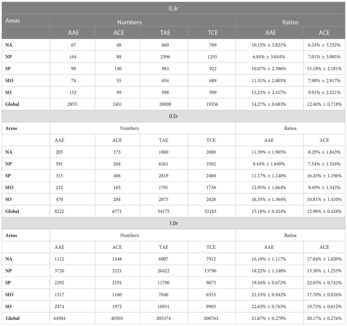
Table 1 The numbers and ratios of abnormal eddies with different relative radius in five regions and globally.

4.2. Eddy-induced depth of the mixed layer

4.2.1. Seasonal and regional variability of eddy influence on MLD

To quantitatively study the effects of eddies on vertical shifts in ML, MLD anomalies are obtained via the removal of the background field from MLD. According to Eq. (6), the global average of MLD anomalies caused by total matching eddies, normal eddies, and abnormal eddies in winter and summer are estimated at 3° × 3° spatial resolution, as shown in Figure 5.

FIGURE 5

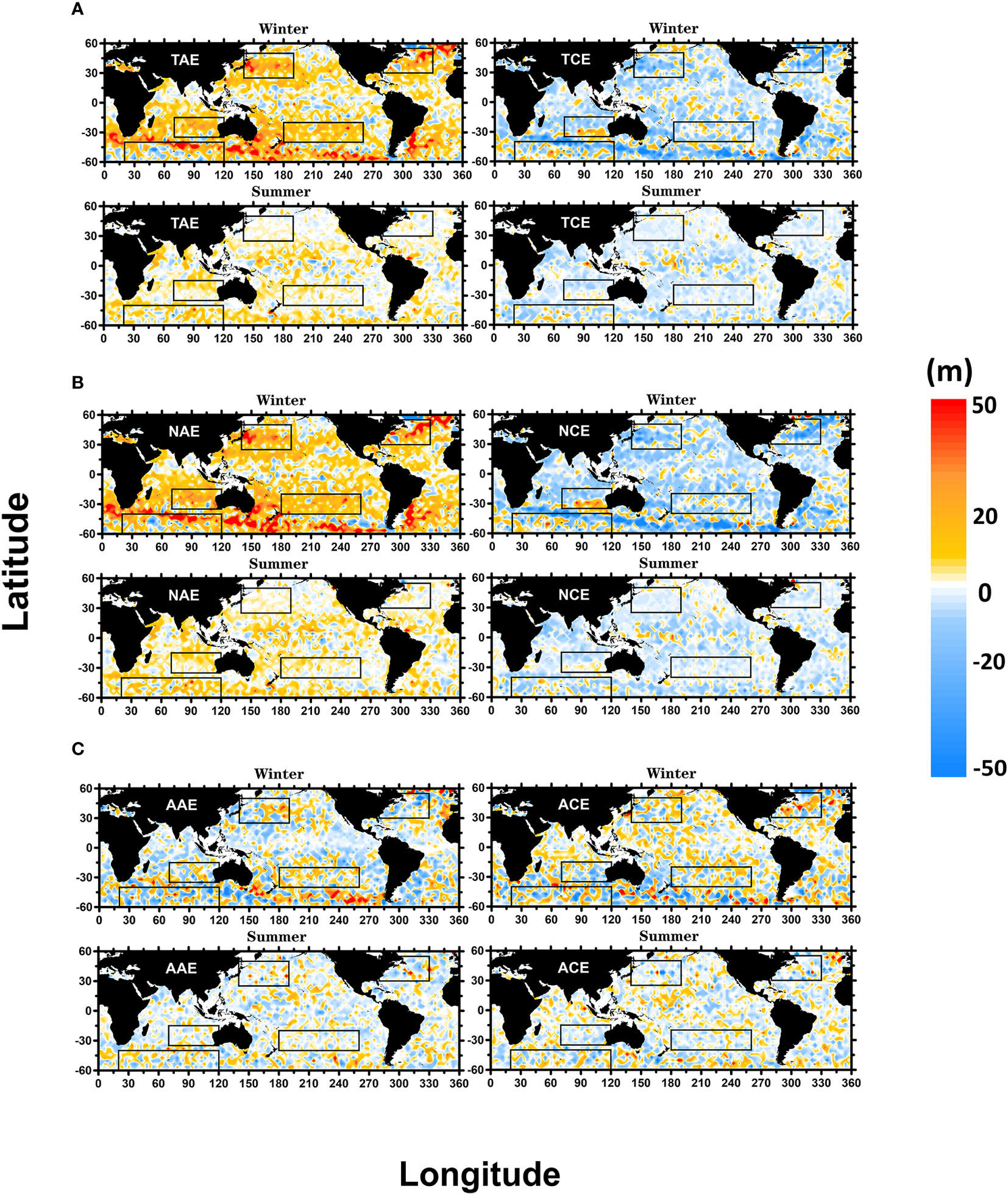
Figure 5 Eddy-induced MLD anomalies (MLD anomalies) mapped to a global 3° × 3° grid between 60°N and 60°S. (A–C) represent total, normal and abnormal eddies, respectively. The black box area represents five areas: NA, NP, SP, SIO, and SO. The upper and lower panels are MLD anomalies inside the eddy in winter (Northern hemisphere: December, January, February; Southern hemisphere: June, July, August) and summer (Northern hemisphere: June, July, August; Southern hemisphere: December, January, February) of each hemisphere, respectively. The left and right panels of each submap are TAE, NAE, AAE and TCE, NCE, ACE, respectively.

Globally, TAE causes positive MLD anomalies, whereas TCE causes negative MLD anomalies, which were more pronounce in winter, in particular, in regions with strong eddy kinetic energy (Figure 5A). In winter and summer, NAE and NCE caused greater deepening and uplifting than the TAE and TCE (Figure 5B). This magnitude of MLD caused by AAE and ACE is weaker than that caused by TAE and TCE and had the opposite signals (Figure 5C). The five representative regions are highlighted by the black boxes in Figure 5, and the northern and southern hemispheres as well as the entire globe were analyzed separately.

The deepening (uplifting) of MLD caused by TAE (TCE) peaked in winter and rapidly decreases with the arrival of summer. NAE (NCE) makes MLD deeper (shallower) than the TAE (TCE), with the difference between NAE and NCE growing larger and more apparent. Compared to TAE (TCE), AAE (ACE) weakened the deepening (uplifting) of MLD. In contrast, the difference between AAE and ACE became smaller and even negative.

To study the characteristics of the effect of eddies (total, normal, and abnormal eddies) on MLD on a monthly scale, the average value of MLD was calculated for each month during 2003-2017, as shown in Figure 6. For example, in the Northern Hemisphere (Figure 6K and Table 2), the maximum value (average) of MLD caused by TAE was ~109 m (~56 m). The maximum (average) value of MLD caused by TCE was ~80 m (~45 m), and the maximum (average) difference was ~28 m (~11 m). NAE (NCE) caused the MLD to be deeper (shallower) up to ~112 m (~79 m) than that caused by TAE (TCE), with the average increasing (decreasing) to ~58 m (~44 m), respectively. The maximum and average differences between NAE and NCE were ~34 m (by ~21%) and ~14 m (by ~27%), respectively. Compared with TAE and TCE, the maximum (average) value of AAE decreased from ~109 m (~56 m) to ~88 m (~48 m), whereas ACE increased from ~80 m (~45 m) to ~96 m (~52 m), respectively. The maximum (average) difference between AAE and ACE decreased to ~-8 m (~-4 m). In this study, the negative sign indicates that the MLD was shallower in AAE than in ACE.

FIGURE 6

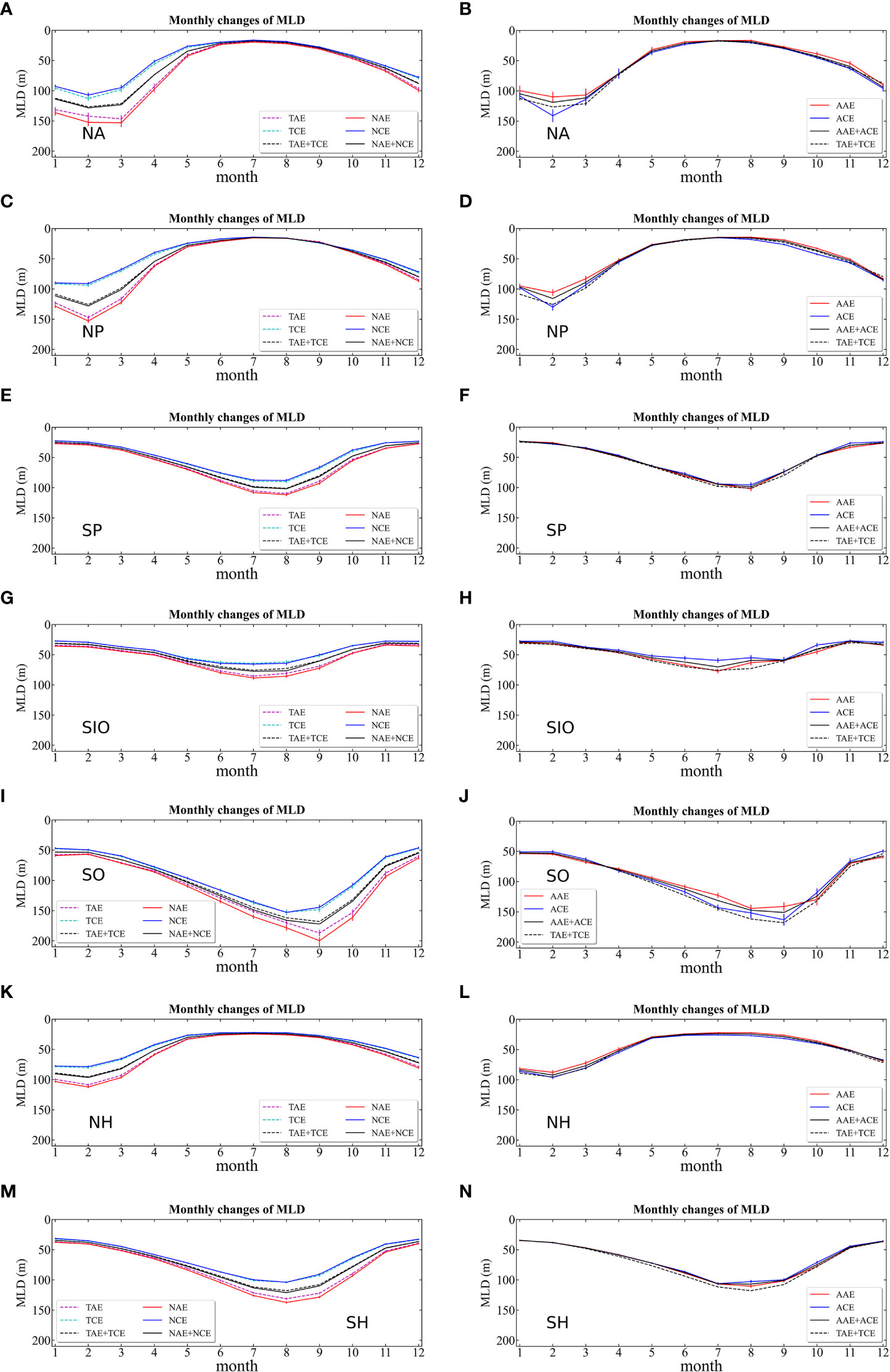
Figure 6 Seasonal cycle of mixed layer depth (MLD) in NA (A, B), NP (C, D), SP (E, F), SIO (G, H), SO (I, J), NH (northern hemisphere) (K, L) and SH (southern hemisphere) (M, N). The solid (dashed) red (magenta) line and solid (dashed) blue (cyan) line represent NAE (TAE) and NCE (TCE) and the solid (dashed) black line indicates the sum of NAE (TAE) and NCE (TCE) in left panels. The solid red (blue) line and solid (dashed) black line in the right panels indicates AAE (ACE) and the sum of AAE (TAE) and ACE (TCE), respectively. The standard error, computed as $\sigma /\sqrt{N}$, where σ is the standard deviation of all MLD observations during each calendar month and N is the number of MLD observations in each month, is indicated by the vertical lines.

TABLE 2

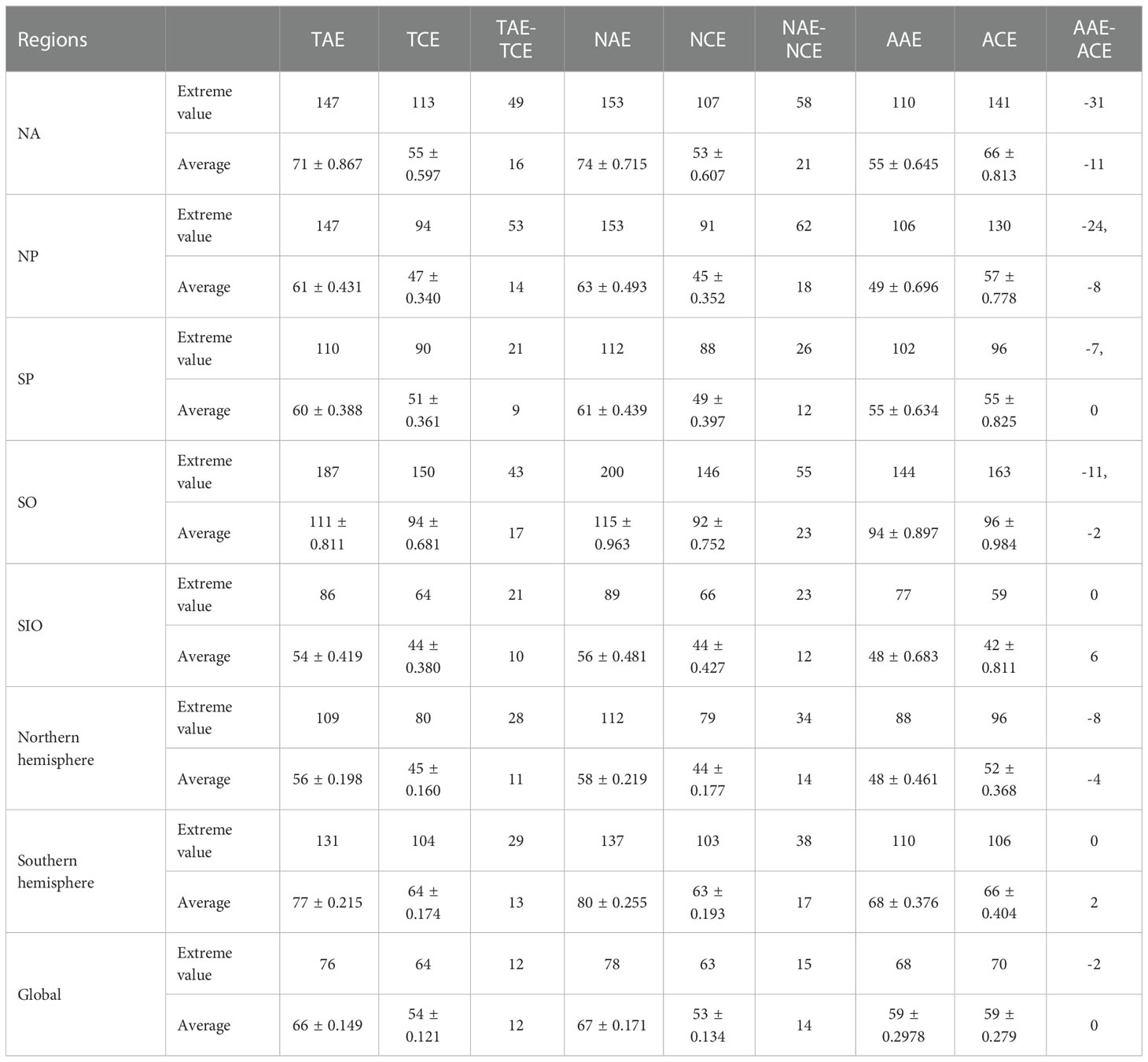
Table 2 Extreme values and averages of mixed layer depth caused by eddies in five regions, northern and southern hemispheres, and globally.

Regionally, the maximum (average) value of the deepening and uplifting of MLD caused by TAE and TCE were ~147 m (~71 m) and ~113 m (~55 m), respectively, in the North Atlantic (Figure 6A and Table 2). The maximum and average differences between TAE and TCE were ~49 m and ~16 m, respectively, with both larger than the corresponding values of the northern and southern hemispheres. NAE and NCE showed deeper and shallower MLD than the TAE and TCE, with the maximum values of ~153 m and ~107 m and with mean values of ~74 m and ~53 m, respectively. The maximum and mean differences between NAE and NCE significantly increased, reaching 58 m and 21 m, respectively, with an increase of ~18% and ~31%, respectively. AAE (ACE) weakened or even reversed the effect of TAE (TCE) on MLD, and their maximum value reached ~110 m (~141 m), and on an average, reached ~55 m (~66 m), respectively. The minimum and average differences between AAE and ACE plunged to a minimum value of the five regions (~-31 m and ~-11 m, respectively). On the contrary, the MLD reached its minimum in summer, but its signal was less significant than its maximum. The MLD shoaled to an average depth< ~20 m, and disturbances caused by eddies were no longer detectable. The minimum value of the MLD was close to ~50 m in the Indian Ocean sector of the Southern Ocean (Figure 6I and Table 2).

4.2.2. The variation of MLD associated with different types of mesoscale eddies MLD anomalies

Overall, positive (negative) MLD anomalies tend to be associated with TAE and TCE. This did not necessarily suggest that TAE (TCE) was only a positive (negative) MLD anomaly. This trend was not unique, as shown in Figure 7A, which indicates that TAE sometimes caused shallower MLD, whereas TCE sometimes caused deeper MLD. The distribution of the ratios showed the asymmetry of the response. In other words, TAE accounted for an increasingly significant share of positive MLD anomalies than the TCE accounting for negative MLD anomalies, as shown by the solid black line in Figure 7C. As can be seen from the solid red line in Figure 7C, the phenomena was more evident in normal eddies. While AAE and ACE accounted for a large proportion of negative and positive anomalies, respectively, AAE (ACE) exhibited more negative (positive) anomalies than the ACE(AAE), as shown in Figure 7B. There were more AAE (ACE) in the negative (positive) anomalies than there were ACE (AAE) anomalies in approximately ±50 m MLD, and subsequently the numbers became comparable. These indicate that abnormal eddies weaken the influence of normal eddies on MLD and even exert the opposite effect.

FIGURE 7

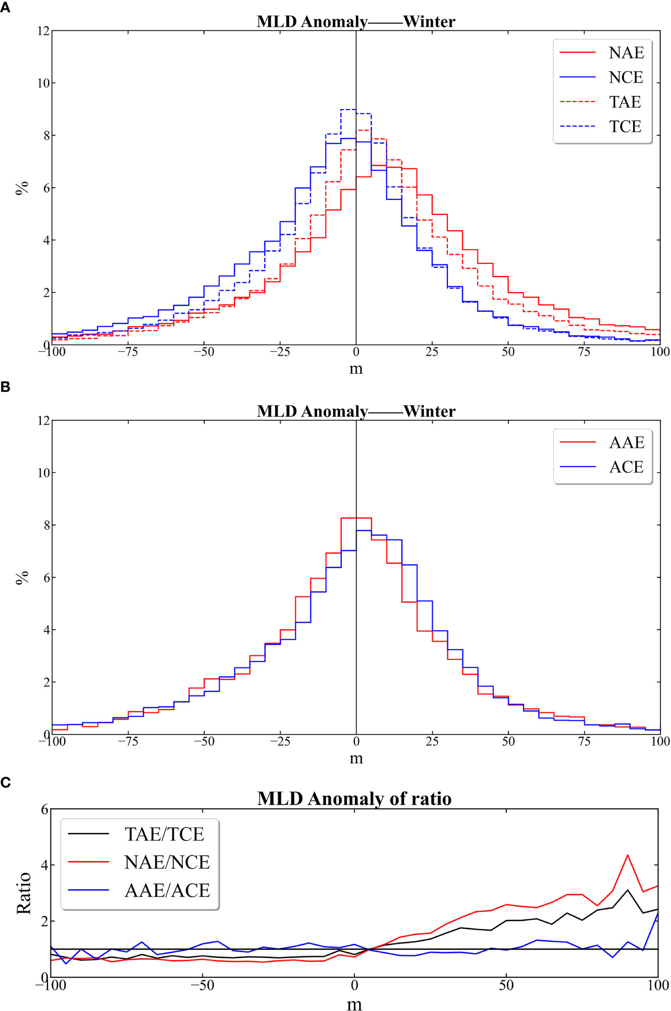
Figure 7 Histogram of global eddy-centric winter time MLD anomalies, including total matching eddies (A), normal eddies (A) and abnormal eddies (B). The solid (dashed) red and blue lines in (A) represent NAE (TAE) and NCE (TCE), the corresponding ratios are shown as solid red and black lines in (C), respectively. The scale of (B) is shown by solid blue lines in (C). The solid red and blue lines represent AAE, and ACE in (B). MLD, mixed layer depth.

Gaube et al. (2019) proposed that MLD anomalies were associated with eddy amplitude. As shown in Figure 8, MLD anomalies approximately showed a linear relationship with eddy amplitude and became more significant as the relative radius decreased in winter. This relationship is more obvious for TAE than TCE. Here, the eddies with amplitude< 2 cm are removed. This pattern was more significant in normal eddies (dashed magenta and cyan in Figure 8). As shown in Figure 8 , the ‘gap’ between normal eddies and total matching eddies was more significant with the increased relative radius, that is, the number of abnormal eddies increased with the rise of relative radius, as shown in Table 1. According to Figure 8 (the dashed red and blue lines), as the relative radius grew smaller, the relationship between MLD anomaly and abnormal eddy amplitude fluctuated, and the effect grew subtle. Overall, AAE (ACE) weakened the deepening (uplifting) effect of MLD.

FIGURE 8

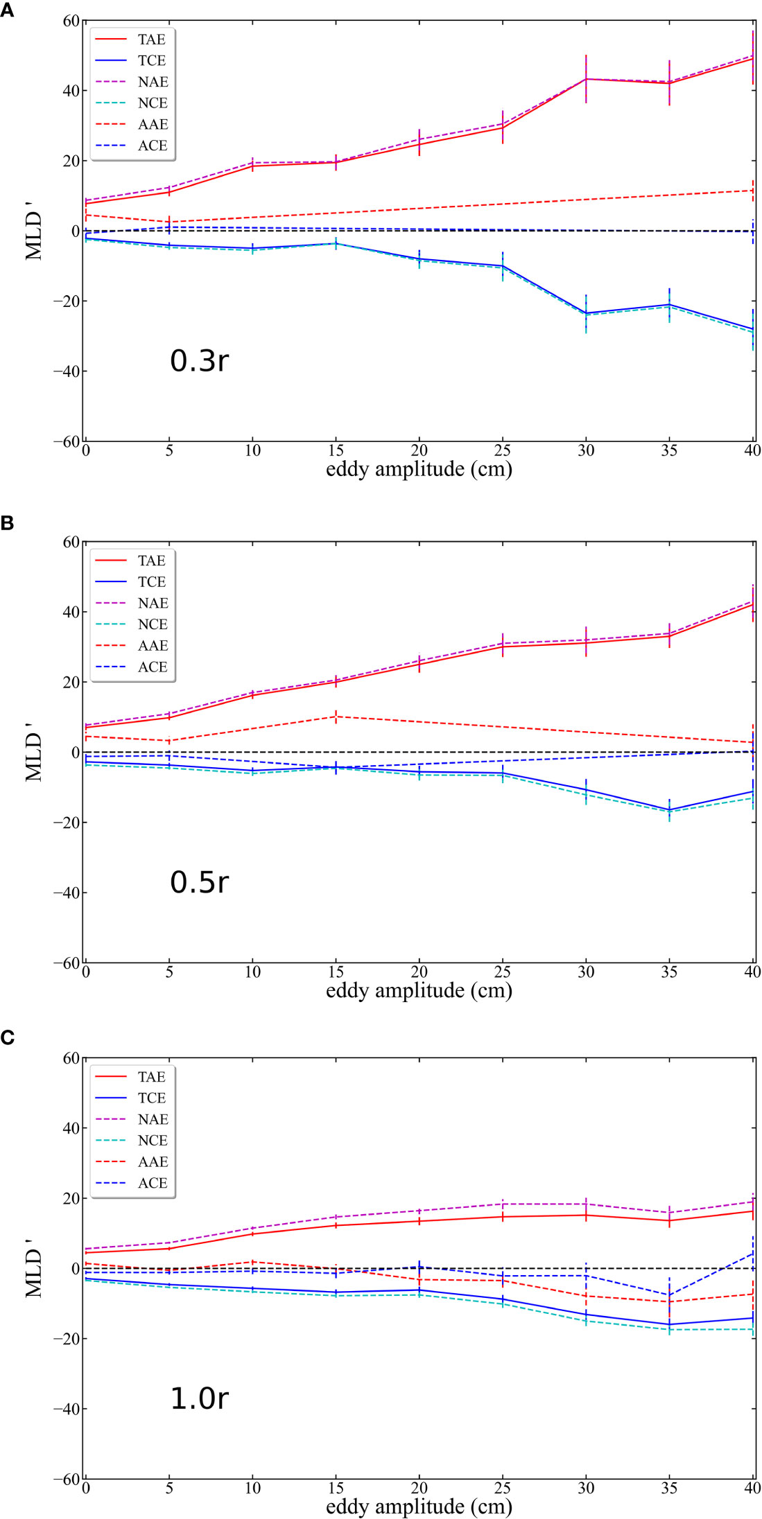
Figure 8 Average winter MLD anomalies (MLD anomalies) as a function of eddy amplitude. (A–C) mean 0.3r, 0.5r and 1r, respectively. TAE, TCE, NAE, NCE, AAE and ACE are represented by solid red, solid blue, dashed magenta, dashed cyan, dashed red and dashed blue respectively. MLD, mixed layer depth.

5. Discussion

In this study, the abnormal eddies refer to eddies whose enclosed PDA had an opposite sign concerning their altimeter-identified polarity. In other words, given the Argo perspective, they cannot be classified as eddies with the same polarity, as shown in Figure 3. Identifying abnormal eddies based on PDA was an essential method in this study, which was different from the previous method based on SST (Sun et al. (2019); Liu et al. (2021); Ni et al. (2021); Sun et al. (2021)). The reason for using PDA was that density is more robust than that in SST in the ocean because SST is susceptible to interference from other factors, such as solar radiation flux, sea surface wind speed, and rainfall, which can affect the identification-related results. Compared with the previous method, the new identification method of abnormal eddies has been improved in two specific ways. First, the abnormal rate was as high as 32% according to Liu et al. (2021). However, the ability of an altimeter ability to identify eddies was relatively stable; hence, their result appeared to be less reasonable. In the present study, the abnormal rate was about 20%, which was more convincing than their results. Second, this study showed a lower abnormal rate in the western boundary current regions because the energy and amplitude of the eddies in these regions are relatively large and cause a stronger PDA signal. Therefore, these places are less likely to be misclassified, which was absent in the results of Liu et al. (2021). Argo-based eddy identification can compensate for the lack of altimetry, partially rectifying its ineffectiveness in low-latitude areas. In particular, the altimeter misclassifies the polarity of the eddies in the oceanic range by approximately 4.3% (Chen et al., 2021a). The abnormal eddies can be divided into AAE and ACE according to the sign of PDAs. This study showed that 21.67% of TAE and 20.17% of TCE were abnormal. As evidenced in Figure 4 and Table 1, abnormal eddies were primarily concentrated in the tropical regions, confirming that altimeter-based eddy identification was less effective in low-latitude areas, which was consistent with the results of Ni et al. (2021) and Chen et al. (2021a). The generation mechanisms for AAE and ACE were also discussed in this study. (1) In tropical regions, where the seawater stratification is strong, and the eddy energy is weaker, less variation in the potential density was caused by the eddy pump. (2) Cyclonic and anticyclonic eddies were misclassified by the altimeter due to its sparse sampling and the weakened Coriolis force. (3) The abnormal eddy may be rendered by the eddy-wind interaction and unstable and complex for the boundary current. For example, the abnormal rate of AAE and ACE can reach 22.63% and 19.75% in the Indian Ocean sector of the Southern Ocean, respectively. As shown in Table 1, the closer to the eddy center, the lower the abnormal rate, which may be due to the strong kinetic energy of the eddy within 0.5r, and the resulting signal was also strong. With the increase relative radius, the eddy kinetic energy gradually weakened, and the abnormal rate gradually increased. The analysis of the error of the abnormal rate (Er) indicated that the error of the abnormal rate gradually increased with the increased relative radius. When r = 1, Er could reach 50%, and Er was less than 10% when r< 0.5. The calculation method assumes the abnormal rate within 0.1r as the reference value. Subsequently, the difference between the abnormal rate and the reference value was divided by the reference value as the error of the abnormal rate (not shown here). Thus, a suitable relative radius, such as 0.5 r, can be appropriately chosen as the criterion for differentiation when abnormal eddies are identified. In this study, the relative radii were calculated taking into account the irregular shape of the eddies considering the Argo fell inside the eddy, r< 1. If the eddies were calculated based on the normalized circle radius, Argo falling outside the eddies was also considered as the internal case. In contrast, the case where Argo fell inside the eddies was considered external.

According to Figures 5, 6, both abnormal and total matching eddies showed the most significant disturbances to MLD in winter. The MLD amplitude caused by abnormal eddy was smaller than the total matching eddy currents in most areas, with the opposite signal appearing. When the abnormal eddies were removed, the results showed that the normal eddies modulate MLD more significantly than the total matching eddies (Figures 5B, 6). From the perspective of eddy-induced MLD, the deeper (shallower) ML in TAE (TCE) was primarily explained by the enhanced (suppressed) ocean convection triggered by anomalous air-sea heat loss (gain) that resulted from positive (negative) SST anomalies associated with TAE (TCE) (Williams, 1988; Hausmann et al., 2017; Gaube et al., 2019). In contrast, the average MLD anomalies caused by AAE and ACE were found to be much smaller in magnitude and even appear as opposite signals. This result may be due to the opposite PDA of AAE and ACE compared to those of TAE and TCE, leading to weaker surface turbulent heat flow anomalies or even opposite signals on AAE and ACE. Subsequently, this resulted in weaker anomalous convective mixing in the surface layers of AAE and ACE. As expect, there was more than one reason for this, which has motivated further research and exploration. The effect of normal and abnormal eddies on MLD showed inter-annual variability, as shown in Figure 9. The northern and southern hemispheres showed an approximate mirror symmetry which also indicated a clear seasonality. In the northern hemisphere, the MLD variation caused by total matching and normal eddies gradually decreased, whereas this variation became less evident in the southern hemisphere. This pattern was also observed for abnormal eddies although their number was small, and their fluctuation was less stable. This phenomenon may be related to the difference in land area and global warming between the northern and southern hemispheres, which needs to be explored in future studies. In Figure 7, the number of TAE in positive MLD anomalies was greater than that of TCE in negative MLD anomalies, and the normal eddy made this effect more pronounced. This reveals that a considerable number of abnormal eddies have weakened or even reversed eddy-induced variation in MLD anomalies, which in turn verified the reliability of our identification method. We can infer from the relationship between eddy amplitude, MLD anomalies (Figure 8), and Table 1 that the closer to the eddy center the Argo profile was, the greater the vertical velocity and flux caused by the eddies, as well as the stronger the temperature and salt anomaly signals inside the eddies were. Thus, identifying the eddies was more accurate with the decreasing relative radius. Integrating the upper and lower limit intervals of the eddy core depth serves to identify abnormal eddies. Therefore, some MLDs caused by eddies located at the upper limit of eddy core depth were not affected by it.

FIGURE 9

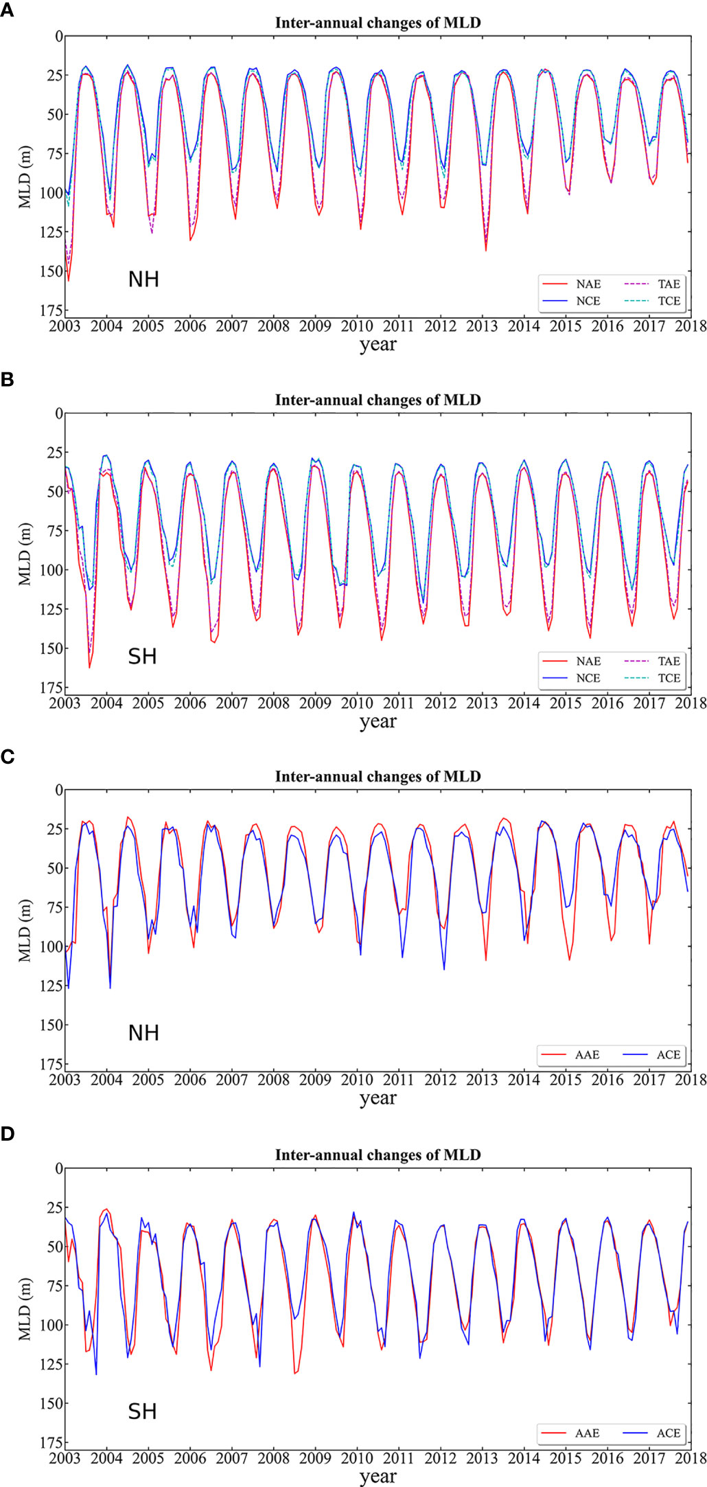
Figure 9 Inter-annual variability of eddies-induced MLD in NH (northern hemisphere) and SH (southern hemisphere). The solid (dashed) red (magenta) line and solid (dashed) blue (cyan) line represent NAE (TAE) and NCE (TCE) in (A, B) The solid red (blue) line in (C, D) indicates AAE (ACE), respectively.

In summary, the abnormal eddies were identified based on the finite Argo density profile, and some eddies without Argo inside them are not identifiable. Calculating MLD climatology was also important for MLD anomalies. The number of Argo profiles directly affected the resolution selection, which determined number and extent of each grid. As the number of Argo continues to increase, the number of eddies matched will increase, and the resolution will become finer. The threshold value selected in the methodology was 0, which can lead to misclassification, in particular, for relatively weak-signal eddies. It is also necessary to consider the distance between the Argo profile and the eddy center because the closer to the eddy center it was, the stronger the signal and the more accurate the results were. For an abnormal eddy, the closer the Argo profile is to the eddy center, the higher its probability of being identified as an abnormal eddy was. Correspondingly, if it was a normal eddy, the closer the Argo profile was to the eddy center, the lower its probability of being identified as an abnormal eddy was. The results indicated that some abnormal eddies exhibit similar properties to normal eddies, which in turn showed that the abnormal eddies were not entirely separated from the normal eddies. In terms of the methods for calculating eddy-induced MLD, there is no guarantee that the impact of other factors on MLD can be removed entirely, such as air-sea heat flux, Ekman transport, and ocean advection and entrainment. Accurately quantifying the net effect of the eddies on the MLD is a question for future research. In some seasons and regions where the changes in MLD are small, the vertical resolution of the Argo profiles needs to be appropriately adjusted for different conditions. In future research, we will continue to optimize the methodology and consider the issues discussed above to ensure that the identified abnormal eddies are more accurate. These will also provide new insights for future research.

The effects of normal and abnormal eddies on other factors are also approximately opposite, and their effects have regional and seasonal characteristics. Whether normal and abnormal eddies conduct regionally or seasonally in oceanographic studies should be considered. The discovery of abnormal eddies enriches the research content of eddy dynamics. The detailed discussion of the four types of eddies in the global region aid to deepen the understanding of global oceanography. Abnormal eddies can also have some influence on the climate. The abnormal eddies are usually the opposite of the latent heat flux (LHF) and sensible heat flux (SHF) of normal eddies. The peak magnitude of LHF anomalies associated with abnormal eddies is roughly half of those associated with total eddies. The eddy-induced SHF anomalies are almost identical to those of LHF anomalies, except for at a smaller magnitude (Ni et al., 2021). Physically, positive eddy SST anomalies induce anomalous upward surface turbulent heat fluxes, strengthening near-surface wind and wind stress, thus enhancing turbulent mixing and downward momentum transport in the atmospheric boundary layer (Chelton and Xie, 2010; Frenger et al., 2013; Gaube et al., 2015). This mechanism works regardless of whether the eddy is normal or abnormal (Liu et al., 2021; Ni et al., 2021). This is particularly significant in localized areas. More accurate maritime weather forecasts that consider the influence of abnormal eddies on atmospheric variables should be established (Chelton and Xie, 2010; Frenger et al., 2013). In addition, heat and material transports induced by eddies (Boas et al., 2015), in particular, those modulated by abnormal eddies and their generation mechanisms, are worthy of further investigation.

6. Conclusion

Using potential density based on the global Argo dataset spanning 15 years, the results indicate that abnormal eddies are surprisingly abundant in the global ocean, and ACE (AAE) account for approximately 20.17% (21.67%) of TCE (TAE). They are more abundant in the tropical regions than in the boundary current and strong eddy kinetic energy regions. Their generation mechanisms were described in the Introduction and Discussion sections. The changes in MLD caused by normal and abnormal eddies were estimated separately. The results showed that AAE (ACE) attenuated the deepening (uplifting) effect of TAE (TCE) on MLD and even plays the opposite role in some areas. For normal eddies, the impacts of NAE and NCE were more significant on MLD than those of TAE and TCE due to the difference between the PDAs inside the normal and abnormal eddies.

The results showed that abnormal and normal eddies may play a distinct role in regulating MLD even in the air-sea system (Chelton and Xie, 2010; Frenger et al., 2013; Boas et al., 2015). The number of normal and abnormal eddies observed in the global ocean may be related to instability of ocean currents, which reflects their long-term variation trend in the global ocean. Most of the current research does not consider the effect of abnormal eddies, which leads to inaccurate results, and the existence of AAE and ACE conceals the different ocean characteristics. Abnormal eddies significantly influence the transportation of mass (Pickart et al., 2005; Mathis et al., 2007; Everett et al., 2012), ocean circulation (Shimizu et al., 2001), and air-sea interaction (Leyba et al., 2017; Liu et al., 2020). Consequently, abnormal eddies need to be appropriately considered when the role of ocean eddies in the Earth’s climate system is assessed and quantified. With the launch of the Surface water and ocean topography satellite (Morrow et al., 2019) and the improvement of resolution and technology, not only can more and smaller scale eddies be identified more accurately but also quantitative studies of MLD and sea-air systems are becoming increasingly accurate.

Data availability statement

The original contributions presented in the study are included in the article/supplementary material. Further inquiries can be directed to the corresponding author.

Author contributions

JH performed algorithm, software, validation, data curation, visualization, writing of the original draft, writing review and editing. JY contributed to methodology, conceptualization and supervision. GC provided ideas for comment responses and funding acquisition. All authors contributed to the article and approved the submitted version.

Funding

This research was jointly supported by Laoshan Laboratory Science and Technology Innovation Project (No. LSKJ202201302), The National Natural Science Foundation of China (Grant No. 42030406), The International Research Center of Big Data for Sustainable Development Goals (No. CBAS2022GSP01), and Ocean University of China (Grant No. 202251004).

Conflict of interest

The authors declare that the research was conducted in the absence of any commercial or financial relationships that could be construed as a potential conflict of interest.

Publisher’s note

All claims expressed in this article are solely those of the authors and do not necessarily represent those of their affiliated organizations, or those of the publisher, the editors and the reviewers. Any product that may be evaluated in this article, or claim that may be made by its manufacturer, is not guaranteed or endorsed by the publisher.

References

Belcher S. E., Grant A. L. M., Hanley K. E., Fox-Kemper B., Van Roekel L., Sullivan P. P., et al. (2012). A global perspective on langmuir turbulence in the ocean surface boundary layer. Geophysical Res. Lett. 39. doi: 10.1029/2012GL052932

CrossRef Full Text | Google Scholar

Boas A. B. V., Sato O. T., Chaigneau A., Castelao G. P. (2015). The signature of mesoscale eddies on the air-sea turbulent heat fluxes in the south Atlantic ocean. Geophysical Res. Lett. 42, 1856–1862. doi: 10.1002/2015GL063105

CrossRef Full Text | Google Scholar

Carton J. A., Grodsky S. A., Liu H. (2008). Variability of the oceanic mixed layer 1960-2004. J. Climate 21, 1029–1047. doi: 10.1175/2007JCLI1798.1

CrossRef Full Text | Google Scholar

Chelton D. B., Schlax M. G., Samelson R. M. (2011). Global observations of nonlinear mesoscale eddies. Prog. Oceanography 91, 167–216. doi: 10.1016/j.pocean.2011.01.002

CrossRef Full Text | Google Scholar

Chelton D. B., Xie S. P. (2010). Coupled ocean-atmosphere interaction at oceanic mesoscales. Oceanography 23, 52–69. doi: 10.5670/oceanog.2010.05

CrossRef Full Text | Google Scholar

Chen D., Busalacchi A. J., Rothstein L. M. (1994). The roles of vertical mixing, solar-radiation, and wind stress in a model simulation of the Sea-surface temperature seasonal cycle in the tropical pacific-ocean. J. Geophysical Research-Oceans 99, 20345–20359. doi: 10.1029/94JC01621

CrossRef Full Text | Google Scholar

Chen G., Chen X. Y., Huang B. X. (2021a). Independent eddy identification with profiling argo as calibrated by altimetry. J. Geophysical Research-Oceans 126 (1). doi: 10.1029/2020JC016729

CrossRef Full Text | Google Scholar

Chen X. Y., Li H. T., Cao C. C., Chen G. (2021b). Eddy-induced pycnocline depth displacement over the global ocean. J. Mar. Syst. 221, 103577. doi: 10.1016/j.jmarsys.2021.103577

CrossRef Full Text | Google Scholar

Chen G., Yu F. J. (2015). An objective algorithm for estimating maximum oceanic mixed layer depth using seasonality indices derived from argo temperature/salinity profiles. J. Geophysical Research-Oceans 120, 582–595. doi: 10.1002/2014JC010383

CrossRef Full Text | Google Scholar

Chereskin T. K., Roemmich D. (1991). A comparison of measured and wind-derived ekman transport at 11\u00b0N in the Atlantic ocean. J. Phys. Oceanogr. 21, 869–878. doi: 10.1175/1520-0485(1991)021<0869:ACOMAW>2.0.CO;2

CrossRef Full Text | Google Scholar

Chu P. C., Fan C. W. (2010). Optimal linear fitting for objective determination of ocean mixed layer depth from glider profiles. J. Atmospheric Oceanic Technol. 27, 1893–1898. doi: 10.1175/2010JTECHO804.1

CrossRef Full Text | Google Scholar

CMEMS (2019). Product user manual for Sea level SLA products. CMEMS-SLPUM 008, 032–062.

Google Scholar

de Boyer Montegut C., Madec G., Fischer A. S., Lazar A., Iudicone D. (2004). Mixed layer depth over the global ocean: An examination of profile data and a profile-based climatology. J. Geophysical Research-Oceans 109 (C12). doi: 10.1029/2004JC002378

CrossRef Full Text | Google Scholar

de Marez C., L'hegaret P., Morvan M., Carton X. (2019). On the 3D structure of eddies in the Arabian Sea. Deep-Sea Res. Part I-Oceanographic Res. Papers 150, 103057. doi: 10.1016/j.dsr.2019.06.003

CrossRef Full Text | Google Scholar

Dufois F., Hardman-Mountford N. J., Greenwood J., Richardson A. J., Feng M., Herbette S., et al. (2014). Impact of eddies on surface chlorophyll in the south Indian ocean. J. Geophysical Research-Oceans 119, 8061–8077. doi: 10.1002/2014JC010164

CrossRef Full Text | Google Scholar

Everett J. D., Baird M. E., Oke P. R., Suthers I. M. (2012). An avenue of eddies: Quantifying the biophysical properties of mesoscale eddies in the Tasman Sea. Geophysical Res. Lett. 39, n/a–n/a. doi: 10.1029/2012GL053091

CrossRef Full Text | Google Scholar

Faghmous J. H., Frenger I., Yao Y. S., Warmka R., Lindell A., Kumar V. (2015). A daily global mesoscale ocean eddy dataset from satellite altimetry. Sci. Data 2 (1), 150028. doi: 10.1038/sdata.2015.28

PubMed Abstract | CrossRef Full Text | Google Scholar

Ferrari R., Wunsch C. (2010). The distribution of eddy kinetic and potential energies in the global ocean. Tellus Ser. a-Dynamic Meteorology Oceanography 62, 92–108. doi: 10.3402/tellusa.v62i2.15680

CrossRef Full Text | Google Scholar

Frenger I., Gruber N., Knutti R., Munnich M. (2013). Imprint of southern ocean eddies on winds, clouds and rainfall. Nat. Geosci. 6, 608–612. doi: 10.1038/ngeo1863

CrossRef Full Text | Google Scholar

Gaube P., Chelton D. B., Samelson R. M., Schlax M. G., O'neill L. W. (2015). Satellite observations of mesoscale eddy-induced ekman pumping. J. Phys. Oceanography 45, 104–132. doi: 10.1175/JPO-D-14-0032.1

CrossRef Full Text | Google Scholar

Gaube P., Chelton D. B., Strutton P. G., Behrenfeld M. J. (2013). Satellite observations of chlorophyll, phytoplankton biomass, and ekman pumping in nonlinear mesoscale eddies. J. Geophysical Research-Oceans 118, 6349–6370. doi: 10.1002/2013JC009027

CrossRef Full Text | Google Scholar

Gaube P., Mcgillicuddy D. J., Moulin A. J. (2019). Mesoscale eddies modulate mixed layer depth globally. Geophysical Res. Lett. 46, 1505–1512. doi: 10.1029/2018GL080006

CrossRef Full Text | Google Scholar

Hausmann U., Mcgillicuddy D. J., Marshall J. (2017). Observed mesoscale eddy signatures in southern ocean surface mixed-layer depth. J. Geophysical Research-Oceans 122, 617–635. doi: 10.1002/2016JC012225

CrossRef Full Text | Google Scholar

Holte J., Talley L. (2009). A new algorithm for finding mixed layer depths with applications to argo data and subantarctic mode water formation. J. Atmospheric Oceanic Technol. 26, 1920–1939. doi: 10.1175/2009JTECHO543.1

CrossRef Full Text | Google Scholar

Holte J., Talley L. D., Gilson J., Roemmich D. (2017). An argo mixed layer climatology and database. Geophysical Res. Lett. 44, 5618–5626. doi: 10.1002/2017GL073426

CrossRef Full Text | Google Scholar

Kadko D., Pickart R. S., Mathis J. (2008). Age characteristics of a shelf-break eddy in the western Arctic and implications for shelf-basin exchange. J. Geophysical Research-Oceans 113 (C2). doi: 10.1029/2007JC004429

CrossRef Full Text | Google Scholar

Kara A. B., Rochford P. A., Hurlburt H. E. (2000). An optimal definition for ocean mixed layer depth. J. Geophysical Research-Oceans 105, 16803–16821. doi: 10.1029/2000JC900072

CrossRef Full Text | Google Scholar

Klein P., Lapeyre G. (2009). The oceanic vertical pump induced by mesoscale and submesoscale turbulence. Annu. Rev. Mar. Sci. 1, 351–375. doi: 10.1146/annurev.marine.010908.163704

CrossRef Full Text | Google Scholar

Klein P., Treguier A. M., Hua B. L. (1998). Three-dimensional stirring of thermohaline fronts. J. Mar. Res. 56, 589–612. doi: 10.1357/002224098765213595

CrossRef Full Text | Google Scholar

Kouketsu S., Tomita H., Oka E., Hosoda S., Kobayashi T., Sato K. (2012). The role of meso-scale eddies in mixed layer deepening and mode water formation in the western north pacific. J. Oceanography 68, 63–77. doi: 10.1007/s10872-011-0049-9

CrossRef Full Text | Google Scholar

Le Vu B., Stegner A., Arsouze T. (2018). Angular momentum eddy detection and tracking algorithm (AMEDA) and its application to coastal eddy formation. J. Atmospheric Oceanic Technol. 35, 739–762. doi: 10.1175/JTECH-D-17-0010.1

CrossRef Full Text | Google Scholar

Leyba I. M., Saraceno M., Solman S. A. (2017). Air-sea heat fluxes associated to mesoscale eddies in the southwestern Atlantic ocean and their dependence on different regional conditions. Climate Dynamics 49, 2491–2501. doi: 10.1007/s00382-016-3460-5

CrossRef Full Text | Google Scholar

Liu Y. J., Chen G., Sun M., Liu S., Tian F. L. (2016). A parallel SLA-based algorithm for global mesoscale eddy identification. J. Atmospheric Oceanic Technol. 33, 2743–2754. doi: 10.1175/JTECH-D-16-0033.1

CrossRef Full Text | Google Scholar

Liu Y. J., Yu L. S., Chen G. (2020). Characterization of Sea surface temperature and air-Sea heat flux anomalies associated with mesoscale eddies in the south China Sea. J. Geophysical Research-Oceans 125 (4). doi: 10.1029/2019JC015470

CrossRef Full Text | Google Scholar

Liu Y. J., Zheng Q. A., Li X. F. (2021). Characteristics of global ocean abnormal mesoscale eddies derived from the fusion of Sea surface height and temperature data by deep learning. Geophysical Res. Lett. 48 (17). doi: 10.1029/2021GL094772

CrossRef Full Text | Google Scholar

Lorbacher K., Dommenget D., Niiler P. P., Kohl A. (2006). Ocean mixed layer depth: A subsurface proxy of ocean-atmosphere variability. J. Geophysical Research-Oceans 111 (C7). doi: 10.1029/2003JC002157

CrossRef Full Text | Google Scholar

Martin A. P., Richards K. J. (2001). Mechanisms for vertical nutrient transport within a north Atlantic mesoscale eddy. Deep-Sea Res. Part Ii-Topical Stud. Oceanography 48, 757–773. doi: 10.1016/S0967-0645(00)00096-5

CrossRef Full Text | Google Scholar

Mathis J. T., Pickart R. S., Hansell D. A., Kadko D., Bates N. R. (2007). Eddy transport of organic carbon and nutrients from the chukchi shelf: Impact on the upper halocline of the western Arctic ocean. J. Geophysical Research-Oceans 112 (C5). doi: 10.1029/2006JC003899

CrossRef Full Text | Google Scholar

Mcdougall T., Feistel R., Millero F., Jackett D., Spitzer P. (2010). The international thermodynamic equation of seawater 2010 (TEOS-10): Calculation and use of thermodynamic properties. Global ship-based repeat hydrography manual. IOCCP Report No. 14.

Google Scholar

Mcgillicuddy D. J. (2015). Formation of intrathermocline lenses by eddy–wind interaction. J. Phys. Oceanography 45, 606–612. doi: 10.1175/JPO-D-14-0221.1

CrossRef Full Text | Google Scholar

Morrow R., Fu L. L., Ardhuin F., Benkiran M., Chapron B., Cosme E., et al. (2019). Global observations of fine-scale ocean surface topography with the surface water and ocean topography (SWOT) mission. Front. Mar. Sci. 6. doi: 10.3389/fmars.2019.00232

CrossRef Full Text | Google Scholar

Ni Q. B. A., Zhai X. M., Jiang X. M., Chen D. K. (2021). Abundant cold anticyclonic eddies and warm cyclonic eddies in the global ocean. J. Phys. Oceanography 51, 2793–2806. doi: 10.1175/JPO-D-21-0010.1

CrossRef Full Text | Google Scholar

Ohlmann J. C., Siegel D. A., Gautier C. (1996). Ocean mixed layer radiant heating and solar penetration: A global analysis. J. Climate 9, 2265–2280. doi: 10.1175/1520-0442(1996)009<2265:OMLRHA>2.0.CO;2

CrossRef Full Text | Google Scholar

Pickart R. S., Weingartner T. J., Pratt L. J., Zimmermann S., Torres D. J. (2005). Flow of winter-transformed pacific water into the Western Arctic. Deep-Sea Res. Part Ii-Topical Stud. Oceanography 52, 3175–3198. doi: 10.1016/j.dsr2.2005.10.009

CrossRef Full Text | Google Scholar

Rabinovich A. B., Thomson R. E., Bograd S. J. (2002). Drifter observations of anticyclonic eddies near bussol' strait, the kuril islands. J. Oceanography 58, 661–671. doi: 10.1023/A:1022890222516

CrossRef Full Text | Google Scholar

Robinson A. R. (1983). Overview and summary of eddy science (Berlin, Heidelberg: Springer Berlin Heidelberg), 3–15.

Google Scholar

Roemmich D., Johnson G. C., Riser S., Davis R., Gilson J., Owens W. B., et al. (2009). The argo program observing the global ocean with profiling floats. Oceanography 22, 34–43. doi: 10.5670/oceanog.2009.36

CrossRef Full Text | Google Scholar

Shimizu Y., Yasuda I., Ito S. (2001). Distribution and circulation of the coastal oyashio intrusion. J. Phys. Oceanography 31, 1561–1578. doi: 10.1175/1520-0485(2001)031<1561:DACOTC>2.0.CO;2

CrossRef Full Text | Google Scholar

Spall M. A., Pickart R. S., Fratantoni P. S., Plueddemann A. J. (2008). Western Arctic Shelfbreak eddies: Formation and transport. J. Phys. Oceanography 38, 1644–1668. doi: 10.1175/2007JPO3829.1

CrossRef Full Text | Google Scholar

Sun W. J., Dong C. M., Tan W., He Y. J. (2019). Statistical characteristics of cyclonic warm-core eddies and anticyclonic cold-core eddies in the north pacific based on remote sensing data. Remote Sens. 11 (2), 208. doi: 10.3390/rs11020208

CrossRef Full Text | Google Scholar

Sun W. J., Liu Y., Chen G. X., Tan W., Lin X. Y., Guan Y. P., et al. (2021). Three-dimensional properties of mesoscale cyclonic warm-core and anticyclonic cold-core eddies in the south China Sea. Acta Oceanologica Sin. 40, 17–29. doi: 10.1007/s13131-021-1770-x

CrossRef Full Text | Google Scholar

Sun M., Tian F. L., Liu Y. J., Chen G. (2017). An improved automatic algorithm for global eddy tracking using satellite altimeter data. Remote Sens. 9 (3) , 206. doi: 10.3390/rs9030206

CrossRef Full Text | Google Scholar

Talley L. D. (1999). Some aspects of ocean heat transport by the shallow, intermediate and deep overturning circulations. Mech. Global Climate Change at Millennial Time Scales, Geophys. Monogr. 112, 1–22. doi: 10.1029/GM112p0001

CrossRef Full Text | Google Scholar

Thomson R. E., Fine I. V. (2003). Estimating mixed layer depth from oceanic profile data. J. Atmospheric Oceanic Technol. 20, 319–329. doi: 10.1175/1520-0426(2003)020<0319:EMLDFO>2.0.CO;2

CrossRef Full Text | Google Scholar

Tian F. L., Wu D., Yuan L. M., Chen G. (2020). Impacts of the efficiencies of identification and tracking algorithms on the statistical properties of global mesoscale eddies using merged altimeter data. Int. J. Remote Sens. 41, 2835–2860. doi: 10.1080/01431161.2019.1694724

CrossRef Full Text | Google Scholar

Williams R. G. (1988). Modification of ocean eddies by air-sea interaction. J. Geophysical Research: Oceans 93, 15523–15533. doi: 10.1029/JC093iC12p15523

CrossRef Full Text | Google Scholar

Yasuda I. Y., Ito S., Shimizu Y., Ichikawa K., Ueda K., Honma T., et al. (2000). Cold-core anticyclonic eddies south of the bussol' strait in the northwestern subarctic pacific. J. Phys. Oceanography 30, 1137–1157. doi: 10.1175/1520-0485(2000)030<1137:CCAESO>2.0.CO;2

CrossRef Full Text | Google Scholar