 Briannyn L. Woods1*
 Anton P. Van de Putte2,3
 Mark A. Hindell1
 Ben Raymond1,4
 Ryan A. Saunders5
 Andrea Walters1
 Rowan Trebilco6,7
- 1Institute for Marine and Antartic Studies, University of Tasmania, Hobart, TAS, Australia
- 2Royal Belgian Institute for Natural Sciences, OD-Nature, Brussel, Belgium
- 3Marine Biology Lab, Université Libre de Bruxelles, Brussel, Belgium
- 4Australian Antarctic Division, Integrated Digital East Antarctica Program, Kingston, TAS, Australia
- 5British Antarctic Survey, Natural Environment Research Council, Cambridge, United Kingdom
- 6CSIRO, Oceans and Atmosphere, Battery Point, TAS, Australia
- 7Centre for Marine Socioecology, University of Tasmania, Hobart, TAS, Australia
Introduction: Mesopelagic fishes play a central role in the transfer of energy through open-ocean food webs, particularly in the Southern Ocean where they are both important predators of zooplankton and a key prey group for many higher predators. However, they are notoriously difficult to sample, which has limited our understanding of the bio-physical predictors of their abundance and spatiotemporal variability. Species distribution models can be used to help understand species’ ecological requirements by relating records of their presence or abundance to environmental data.
Methods: Here, we used data from Myctobase – a new circumpolar database of mesopelagic fishes – to model patterns in abundance of eight key myctophid species (family Myctophidae) and the genus Bathylagus in the Southern Ocean south of 45°S. We developed species-specific boosted regression tree models to obtain circumpolar predictions of abundance. Average daytime and night-time summer predictions for the period 1997 to 2011 at 0 to 200m depths were generated for each species.
Results: Depth and solar position were important predictors and species were stratified in their depth distribution. For all species, except for G. nicholsi, there was an interaction between depth of capture and solar position, reflecting diel vertical migration. Other important variables included sea surface temperature, dissolved oxygen at 200 m, chlorophyll a, and sea surface height, indicating an association with water mass properties. Circumpolar patterns of abundance varied between species with some displaying affinities for oceanic regions at Antarctic latitudes (e.g., E. antarctica and Bathylagus spp.) or sub-Antarctic latitudes (e.g., K. anderssoni and P. tenisoni); and affinities for shelf regions (e.g., P. boliniand G. nicholsi).
Discussion: Our findings suggest that the abundance of mesopelagic fish is influenced by diel vertical migration and meso- and sub-mesoscale oceanographic features, with the Polar Front being a major delimiting feature. Our study showed contrasting patterns in community composition with higher species diversity north of the Polar Front that might be indicative of latitudinal variability in food web structure. Our spatial analysis is an important step toward resolving what determines important habitat for mesopelagic fishes, providing foundational information for understanding shifting food web dynamics into the future.
1 Introduction
Mesopelagic fish (predominantly inhabiting the mesopelagic zone, 200 – 1000 m) are a central part of open-ocean food webs and play an important role in both top-down and bottom-up ecosystem structuring processes (Griffiths et al., 2013; Caccavo et al., 2021). Myctophids (family Myctophidae) are the most diverse and abundant group of mesopelagic fishes globally, including in the Southern Ocean, where they comprise more than 60 species (Duhamel et al., 2014) and an estimated biomass between 212 and 396 million tonnes (Lubimova et al., 1987), although this is likely to be an underestimate due to previously unaccounted for net avoidance (Kaartvedt et al., 2012). In some regions of the Southern Ocean, particularly the Indian and West Pacific sectors, myctophids are the dominant prey resource sustaining top-predator biomass (McCormack et al., 2019; Saunders et al., 2019; McCormack et al., 2021). In turn, myctophids are important zooplanktivores, consuming copepods, amphipods and euphausiids, including Antarctic krill Euphausia superba (Saunders et al., 2018; Clarke et al., 2020; Riaz et al., 2020). Myctophids are key to linking this secondary productivity to higher predators i.e. flying seabirds, penguins, seals and Patagonian toothfish (e.g., Olsson and North, 1997; Gaskett et al., 2001; Cherel et al., 2002; Lea et al., 2002; Collins et al., 2007; Stowasser et al., 2012; O’Toole et al., 2014). Many species undertake diel vertical migration (DVM), where they reside at depths during the day and migrate to shallower waters at night (Brierley, 2014; Duhamel et al., 2014). DVM is a behavioral adaptation with important implications for prey availability to higher predators and enhances carbon sequestration by active transport of organic carbon from the surface to the deep ocean (Brierley, 2014; Irigoien et al., 2014; Anderson et al., 2018; Saba et al., 2021).
The critical importance of myctophids in Southern Ocean pelagic ecosystems is increasingly well-recognized, however, major gaps remain in our knowledge of their biodiversity, abundance and the processes that shape their distribution (Kaartvedt et al., 2012; Anderson et al., 2018; Caccavo et al., 2021). Their open-ocean habitats are logistically difficult to access and costly to sample given the remoteness of such environments (Rogers, 2015). Mesopelagic fishes are difficult to sample adequately at the ocean basin scale with pelagic nets (Kloser et al., 2009); catch efficiency is known to vary between net types (Pakhomov and Yamamura, 2010) and is poorly constrained for any given net (Davison et al., 2015). In contrast, acoustic methods can rapidly sample vast spatial extents (Benoit-Bird and Lawson, 2016; Dornan et al., 2022), however they are unable to capture changes in community composition (Dornan et al., 2019). Consequently, net sampling remains an important tool for examining patterns in biodiversity, abundance, and community composition (McClatchie et al., 2000; St John et al., 2016).
Species distribution models are a commonly used method in the study of biogeography, ecology, evolution, and conservation biology (Guisan and Zimmermann, 2000; Peterson, 2006; Elith et al., 2008). The overarching objective of species distribution models is to determine species’ ecological requirements by relating records of their presence or abundance to environmental predictors and to provide predictions of species’ geographic distribution (Guisan and Zimmermann, 2000; Peterson, 2006). Such models can provide many important insights to ecological and biogeographical dynamics of communities and broad scale projected species’ distribution under different climate change scenarios (Kissling et al., 2018; Freer et al., 2019; Jetz et al., 2019).
Circumpolar descriptions of mesopelagic fish distribution are most often based on occurrence (presence-absence or presence-only) data (Hulley and Duhamel, 2011; Koubbi et al., 2011b; Duhamel et al., 2014; Freer et al., 2019). Occurrence data are easier to collect compared to abundance data, particularly in logistically difficult to sample environments and are readily available in online data repositories (Kissling et al., 2018; Jetz et al., 2019). These occurrence-based studies have demonstrated the importance of meso- and sub-mesoscale oceanographic features on community composition where frontal zones are the major delimiting factors to species distributions (Hulley and Duhamel, 2011; Koubbi et al., 2011b; Duhamel et al., 2014; Freer et al., 2019). While a high probability of occurrence provides a broadscale picture of distribution it does not necessarily equate to a high density of individuals or indicate core habitat (Renwick et al., 2012; Johnston et al., 2015). Abundance trends of populations are additionally important to examine when assessing the status of species (O’Grady et al., 2004; Shoo et al., 2005; Clements et al., 2017), in particular for understanding prey fields for higher predators (Green et al., 2020), and the relative importance of different trophic pathways in food webs (Trebilco et al., 2020). A baseline understanding of the patterns in myctophid abundance would also underpin knowledge of how the mesopelagic fish population may change into the future and the implications of such changes to broader food web dynamics (Constable et al., 2014; Rogers, 2015; St John et al., 2016; Hidalgo and Browman, 2019).
Here, we make the important advance of investigating the drivers of circumpolar abundance of key mesopelagic fish species, taking advantage of Myctobase – a new data collation project that integrates and standardizes existing abundance, biomass, biodiversity, and methodological data on Southern Ocean mesopelagic fishes (Woods et al., 2021; Woods et al., 2022). We used data from Myctobase to develop species-specific models of the abundance of eight myctophid species and the genus Bathylagus. We used a set of environmental variables to develop species distribution models and subsequently used these models to obtain a circumpolar prediction of abundance for each species. The specific objectives of this study are to: 1) establish a robust framework for analyzing complex net data from Myctobase, accounting for differences in gear type and spatial and temporal coverage of surveys; 2) describe the environmental, vertical, and geographic patterns of Southern Ocean mesopelagic fish abundance at a circumpolar scale; and 3) compare model outputs with those from previous models based on occurrence data.
2 Materials and methods
2.1 Myctobase: Data collection
Survey data for mesopelagic fish species from midwater trawls in the Southern Ocean were collated in a purpose-built database, Myctobase. A detailed description of the database, including the data collection and processing steps can be found in Woods et al. (2022). The database currently holds 17, 491 records of occurrence from 4780 net hauls conducted across 72 different Southern Ocean research cruises between 1991 and 2019 by eight national research programs (Figure 1). The database includes detailed metadata for each sample (e.g. latitude, longitude, depth, date-time of trawl, net type and volume filtered), as well as taxonomic information, estimated species abundance and length-weight measurements.
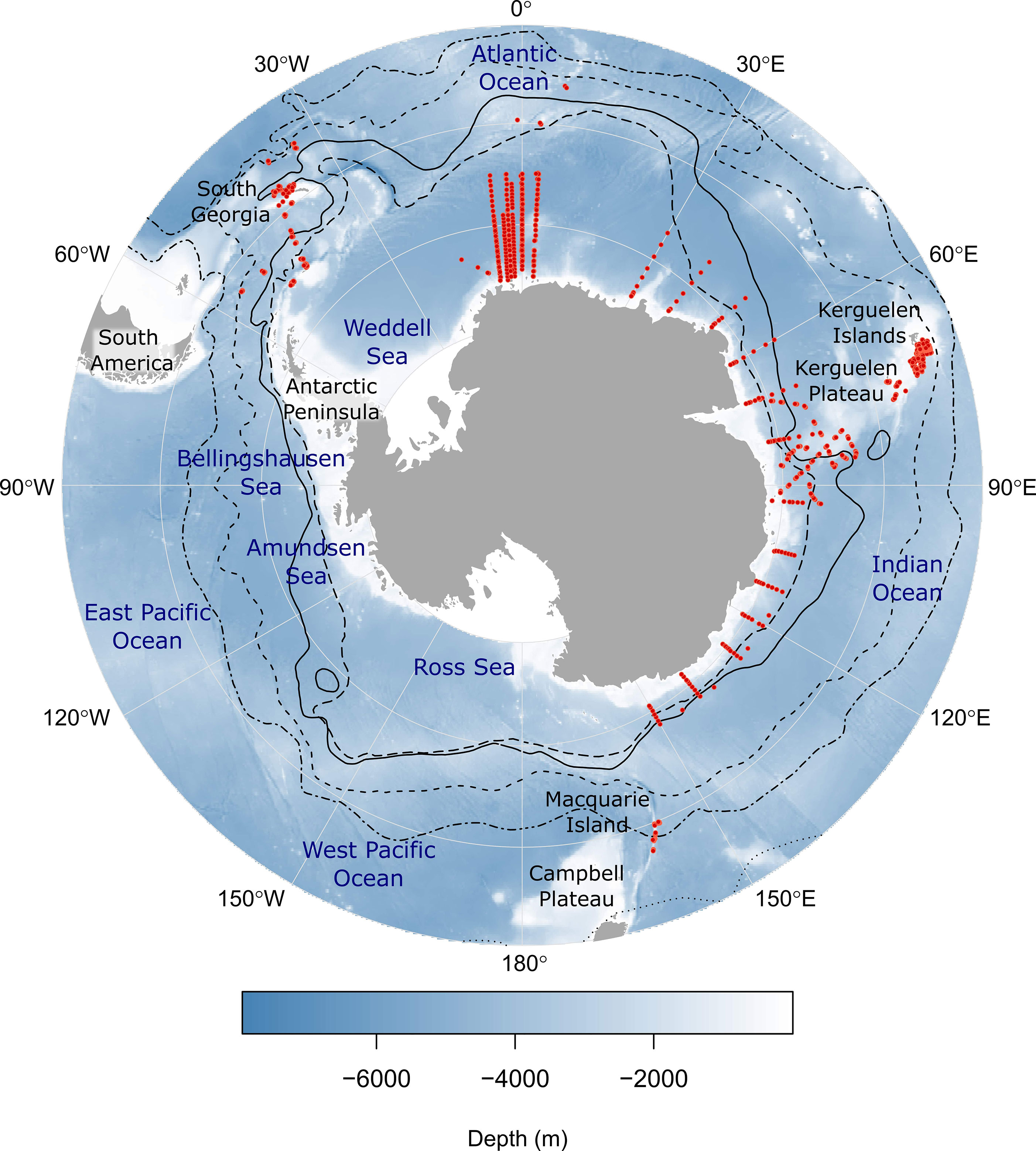
Figure 1 The sampling locations of 1905 mesopelagic trawl nets (red points) from which abundance records of mesopelagic fish species were used for this study. Black lines indicate mean frontal positions (Orsi et al., 1995). Starting from the outer line, frontal features are as follows: Subtropical Front (dotted line); sub-Antarctic Front (dash-dot line); Polar Front (dashed line); southern Antarctic Circumpolar Current Front (solid line); southern boundary of the ACC (long-dashed line). Numbered labels around the outside of the map indicate the longitude. Each latitude line represents 10° of latitude where 75°S is at the Antarctic continent and 45°S is at the external line.
Samples were collected from pelagic trawls using opening-closing net systems with a range of net types including Rectangular Midwater Trawl (RMT) and International Young Gadoid Pelagic Trawl (IYGPT) nets, an Isaacs-Kidd Midwater Trawl (IKMT) net and a Matsuda-Oozeki-Hu Trawl (MOHT) net. Detailed information for each net type can be found in Woods et al. (2022). Opening-closing net systems enabled the sampling of discrete depth intervals.
2.2 Species abundance records
This study focused on the eight most abundant myctophid species within Myctobase (Electrona antarctica, E. carlsbergi, Gymnoscopelus braueri, G. fraseri, G. nicholsi, Krefftichthys anderssoni, Protomyctophum bolini and P. tenisoni) and species of the genus Bathylagus (family Bathylagidae). Records for Bathylagus spp. were rarely identified to species level within the database and were grouped and analyzed at the genus level. Abundance records underwent a process of data cleaning and error checking as described in Woods et al. (2022). Target trawls (trawls undertaken on acoustically detected aggregations of fish) were excluded and only data from the most common net types were included (IYGPT with MIDOC, IYGPT, RMT 25 and RMT 8). Abundance was calculated as the number of individuals per filtered volume of water (individuals 1000 m-3) for each net haul.
2.3 Environmental data
We developed species-specific boosted regression tree models to obtain circumpolar predictions of relative abundance. Eleven environmental covariates were used to model the abundance of each species, guided by previous research demonstrating their importance in determining suitable habitat for mesopelagic fish species (Loots et al., 2007; Koubbi et al., 2011b; Flynn and Marshall, 2013; Duhamel et al., 2014; Proud et al., 2017; Freer et al., 2020; Dornan et al., 2022). We predominantly used variables from the top 200 m of the water column. Subsurface (deeper than 200 m) environmental variables have been suggested to be more informative than surface variables (Koubbi et al., 2011b); however, obtaining the appropriate data to achieve this is not always possible as at-depth environmental parameters are often unavailable or unrecorded. Freer et al. (2020) constructed depth-resolved occurrence models for several myctophid species using environmental predictor variables at different depth intervals, but due to the paucity and uncertainty in depth data used for the 3D models they found that this resulted in smaller sample sizes compared to 2D models increasing the uncertainty around predictions. They also showed high overlap between the two types of models in their final outputs, demonstrating that a balance must be struck between the quantity of data versus the quality of observations and that 2D and 3D models are often comparable (Freer et al., 2020). Given these findings, we consider the use of predominantly surface environmental variables in this study to provide a reasonable proxy for preferred conditions of mesopelagic fish species.
Environmental predictors were compiled in the statistical software R, version 4. 0. 4 (R Core Team, 2021) using the raadtools package (Sumner, 2018, Table 1) and the package maptools for solar position (Bivand et al., 2021). Monthly means were used for dynamic environmental variables across the temporal range of the data (January 1991 – February 2016). However, where monthly data were not available, monthly climatologies or annual means were used (e.g. mixed layer depth). All variables were resampled to a 0.1° x 0.1° grid using bi-linear interpolation (Figure S1). This bi-linear interpolation was a necessary step to fill gaps in covariate coverage. While unavoidable, we do acknowledge that this may introduce some bias/error (see discussion for further consideration of the implications of limited data coverage).
We selected physical oceanographic variables such as sea surface temperature, mixed layer depth, sea surface height and vertical velocity to act as proxies for different water masses, mesoscale eddies, and oceanic fronts that can indicate regions of increased primary productivity or influence the transport of taxa through advective processes (Bost et al., 2009, Table 1). We also selected two variables that relate to productivity, chlorophyll-a and particulate organic carbon that can indicate regions of high prey availability (Sokolov and Rintoul, 2007b; Proud et al., 2017).
Catch efficiency varies between net types, which may lead to differences in estimates of abundance (Pakhomov and Yamamura, 2010; Kaartvedt et al., 2012; Irigoien et al., 2014). To account for differences in the catch efficiency between sampling gear, net type and cod-end mesh size were included as categorical predictors for abundance. Further, the minimum and maximum depth of each net haul was included to account for depth preferences and varying DVM behaviors.
Spatial autocorrelation (SAC) is a common characteristic of ecological data. This occurs when observations close to one another have more similar values compared to observations further apart (Crase et al., 2012). Given our data were collected along transects we anticipated the presence of spatial autocorrelation. To account for this, we included an additional term as a predictor in the model (auto-covariate) to specify the relationship between observations at a location and the observations at a neighbouring location. We followed the three-step process outlined in Crase et al. (2012) to fit the models with an auto-covariate term. First, we fitted our full model, without an auto-covariate term, and extracted the residuals from the model for each grid cell. Using these residuals we calculated the auto-covariate with a mean focal operation for a first order neighborhood. The final step was to fit the full model again including the auto-covariate as an explanatory term within the model (Crase et al., 2012).
2.4 Boosted Regression Tree model fitting and evaluation
The boosted regression tree (BRT) modelling technique was used to model and predict the abundance of mesopelagic fish species in the Southern Ocean. BRT is an ensemble method that combines the strengths of many simple models to build a prediction model (Hastie et al., 2001). BRT uses two algorithms to achieve this, simple regression trees and a machine learning technique known as boosting. Simple regression trees partition the response data into subgroups by recursive binary splits as determined by the predictor variables. One of the advantages of regression trees is that they can accommodate missing values within predictor variables by using surrogates (Hastie et al., 2001; Leathwick et al., 2006; Elith et al., 2008). For example, when the best variable to determine the split is missing, the split will be performed on the next best variable. Regression trees structure the data hierarchically, meaning that a response to one input variable will depend on values at higher levels of the tree (Hastie et al., 2001; Elith et al., 2008). An advantage of this is interactions between predictors are automatically modelled. However, less favorably, this can lead to high variability in the final outputs. Any small change in the data can result in a very different series of splits and errors within the data will be propagated to lower levels of the tree (Hastie et al., 2001). However, the second algorithm used in BRT, boosting, reduces the variance introduced by tree-based methods and enhances predictive performance of regression trees (Hastie et al., 2001).
Boosting is a stagewise process in which regression trees are repeatedly fit to the training data and added to the model. At each step of the process, a new tree is added that best reduces the loss function, which is a measure of the loss in predictive performance due to a suboptimal model Hastie et al., 2001; Elith et al., 2008). The first regression tree best reduces the loss function and at each new iteration the emphasis is placed on the more difficult observations to predict by fitting to the residuals of the previous collection of trees (Elith et al., 2008). The resulting output is an additive regression model in which each tree is an individual term (Elith et al., 2008). The BRT modelling approach has been shown to outperform more traditional approaches, such as generalized additive models that aim to fit a single best model (Elith et al., 2006; Escobar-Flores et al., 2018; Guillaumot et al., 2018).
In this study, a BRT model was fitted for each species in the statistical software R, version 4. 0. 4 (R Core Team, 2021) using the gbm package (Ridgeway, 2006) and additional custom functions from Elith et al. (2008). Abundance models were fitted using a Gaussian distribution. Prior to model fitting, abundance data were log transformed to account for the skewed nature of the data. Data were subsequently reverse log-transformed using Duan’s Smearing Estimator (Duan, 1983) for interpretation of model outputs.
Boosted regression trees have three key parameters that must be fine-tuned to prevent over-fitting the models. The learning rate (lr) specifies the amount each new tree will contribute to the growing model; tree complexity (tc), also known as the interaction depth, specifies the number of nodes in a tree that determines the potential for fitting interactions; and the bag fraction (bf) controls the amount of stochasticity within the model by specifying the proportion of data to be randomly selected at each iteration (Elith et al., 2008). The parameters combine to specify the number of trees (nt) needed to achieve the lowest predictive deviance (Elith et al., 2008). To determine optimal parameters for final BRT models, we systematically altered: lr = 0.1, 0.5, 0.01 or 0.05; tc = 1 to 5; and bf = 0.5, 0.7 or 0.8, as recommended in Elith et al. (2008). The resulting candidate models were evaluated using the mean correlation coefficient between observed and predicted values and by comparing the deviance explained of the models resulting from 10-fold cross validation (Leathwick et al., 2006; Elith et al., 2008). The deviance explained is a measure of goodness-of-fit between the predicted and measured values (Elith et al., 2008). This was calculated following Leathwick et al. (2006), where deviance explained (%) = total deviance – CV residual deviance/total deviance x 100. We applied the random 10-fold cross-validation procedure recommended by Elith et al. (2008) where the data were randomly partitioned into testing and training sets. Here, the data were split into ten distinct subsets where the bag fraction determined the size of the subsets. In turn, each subset was used as test data and the remainder as training data (see Table S1 for the final model parameters). Finally, the relative importance of an environmental variable in the final model was based on the number of times it was selected for splitting in individual decision trees, weighted by the squared improvement to the model from each split and averaged across all trees (Friedman and Meulman, 2003; Elith et al., 2008).
Final fitted models (Table S1) were used to obtain circumpolar predictions of the abundance of individual species (areas south of 45°S). Predictions were made for the period of 1997 – 2011 for the summer months of November to February (the period in which most trawl data came from) and averaged to generate an overall summer prediction at 0 – 200 m depths for each species. The epipelagic depth layer (0 – 200 m) was selected for circumpolar predictions to match the common foraging depth of mesopelagic fish predators (Bost et al., 2009; McMahon et al., 2019; Proud et al., 2021). Net type and cod-end mesh were held constant for predictions (RMT 25 with a cod-end mesh of 5 mm) and separate predictions were made for both the daytime (SOLp = 30°) and night-time (SOLp = -30°) periods.
Uncertainty in model predictions were estimated using a bootstrap approach following the procedure outlined in Hindell et al. (2020). Each model was refitted 50 times to a bootstrap sample of the data, and the interquartile range was calculated for each cell from the 50 iterations. To demonstrate the size of the IQR in relation to the mean prediction for each cell, we divided the IQR by the prediction to determine a coefficient of variation. Optimized model parameters were used for each of the 50 iterations and half the data were sampled with replacement to fit the model each time.
3 Results
A total of 5446 records of abundance were analyzed for 8 different myctophid species and the genus Bathylagus from 1905 net trawls (Figure 1; Table S1). Approximately 67% of records were from the Indian sector and 29% were from the Atlantic sector of the Southern Ocean. The remaining 4% of records originated from the West Pacific sector of the Southern Ocean from the Macquarie Island region (Figure 1).
3.1 Model performance and prediction uncertainty
The mean cross-validated correlation coefficients from 10-fold cross validation ranged from a minimum of 0.49 for G. fraseri to a maximum of 0.69 for K. anderssoni explaining 23% and 47% of the deviance, respectively (Figure 2; Table S1). Differences in model performance across species did not appear to be related to differences in sample size (F1,7 = 0.320, r2 = 0.09, p = 0.59; Figure S2). For example, E. antarctica had the largest sample size (n = 1069) and a deviance explained of 39%, while E. carlsbergi had the smallest sample size (n = 337) and the BRT model performed similarly (deviance explained 39%) to that of E. antarctica (Figure S2). Additionally, including a spatial autocorrelation term (SAC) as a predictor in the model did not improve performance (Table S1). As such, we did not include the SAC term in our final predictions.
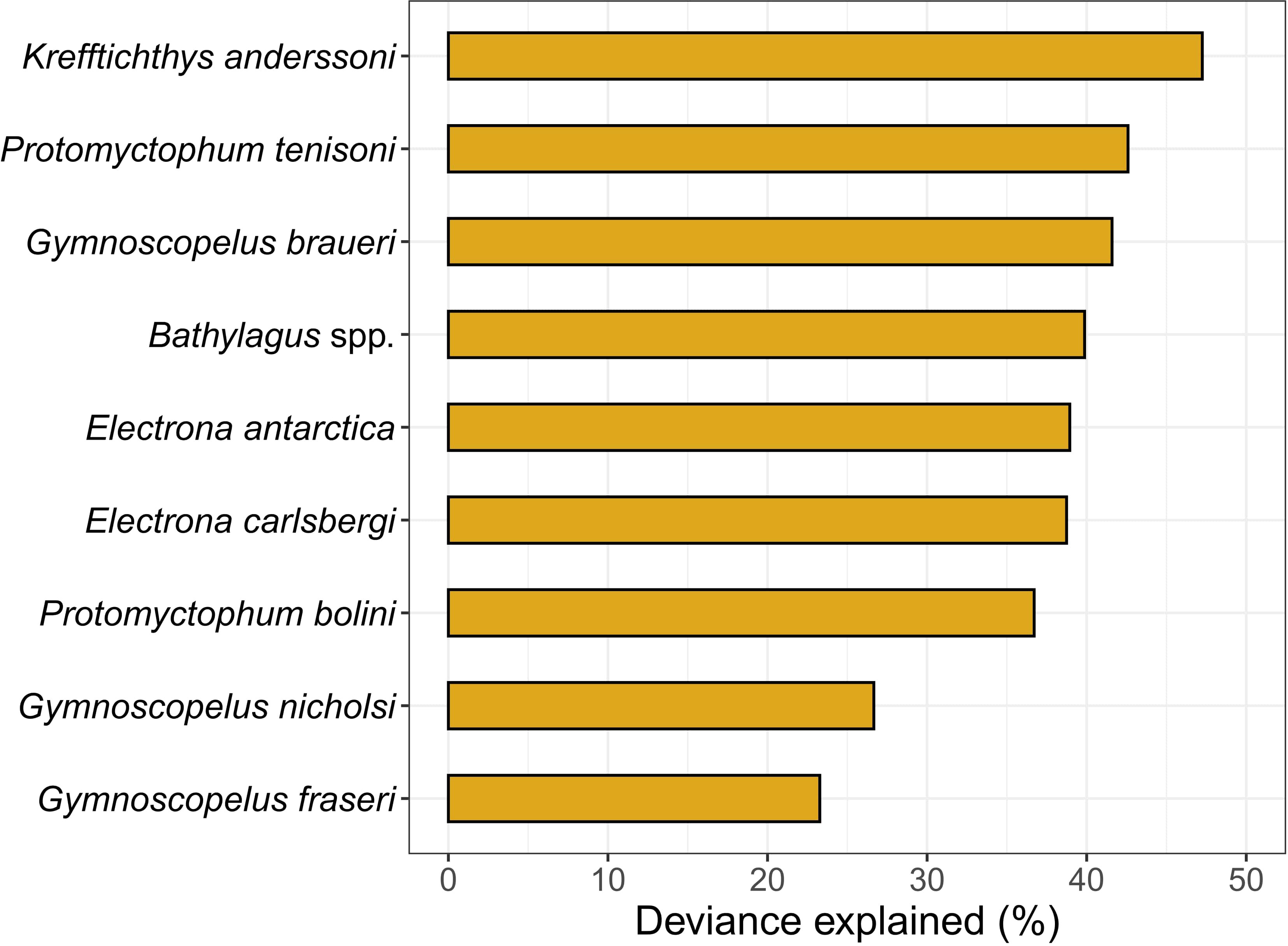
Figure 2 Model performance of Gaussian boosted regression tree models measured as the percent deviance explained, a measure of goodness-of-fit, for nine taxa from ten-fold cross validation.
To assess the robustness of individual BRT models, we analyzed prediction uncertainties using a coefficient of variation. Uncertainties in model predictions were highest for sample data poor regions, for which the predictions were necessarily extrapolations based on geographically distant data from other regions. Furthermore, areas in which abundance predictions were low were more variable compared to areas in which abundance predictions were high (Figure S3). There tended to be less variability for night-time predictions versus daytime. The highest level of uncertainty was seen for E. carlsbergi south of the Polar Front (PF) in the Atlantic Ocean where the IQR was 9 times the mean for some grid cells. Abundance models of Bathylagus spp. had the lowest levels of uncertainty compared to all other myctophid species with a maximum IQR approximately equal to the mean. The region of highest certainty for Bathylagus spp. was the Atlantic Sector south of the PF in areas associated with the highest abundance predictions (Figure S3).
3.2 Environmental predictors
The predictor variables differed in their relative importance (% contribution to the final model) across species (Figure S4). Dissolved oxygen at 200 m (DO200) showed the highest relative contribution score as the most important predictor of abundance for K. anderssoni (48.8%). DO200 also ranked in the top four covariates for two other species, P. bolini (28.4%) and E. antarctica (10.2%). Solar position (SOLp) and the maximum depth of the trawl (DEPTHmax) were consistently within the top four most important variables for predicting the abundance of species (six out of nine species models for SOLp and eight out of nine species models for DEPTHmax). The average contribution of SOLp and DEPTHmax across the nine species models was 10.5% and 13.6%, respectively. Chlorophyll-a concentration (CHLA) also commonly ranked in the top four most important covariates featuring in five out the nine species models with an average contribution of 8.4% across the nine species models. Vertical velocity at 250 m (VEL250) was important only to G. nicholsi ranking in the top four most important covariates with a relative importance of 19.4%. Similarly, particulate organic carbon (POC) was important only to G. braueri (12.1%).
The four most influential predictors for the abundance of each species are shown in Figure 3. Species responses to DO200 (for K. anderssoni, P. bolini and E. antarctica) were similar with the highest abundance predictions across a narrow range of 6 – 7 ml/L (Figure 3) suggesting an affinity for certain water masses. Abundance of E. antarctica and P. bolini increased with increasing CHLA; however, the overall response was more complex for P. tenisoni, E. carlsbergi and G. fraseri. Further, abundance estimates for G. braueri declined with increasing POC, which contrasts with what we might expect as POC is a proxy for productivity, which would indicate areas of high prey abundance (Proud et al., 2017). Sea surface temperature (SST) was important for P. bolini, G. braueri and Bathylagus spp. Physical oceanographic variables such as VEL250, sea surface height gradient (SSHg) and sea surface height anomaly (SSHa) were important for E. carlsbergi, P. tenisoni, G. nicholsi, G. fraseri and Bathylagus spp. suggesting affinities for certain frontal features and mesoscale eddies.
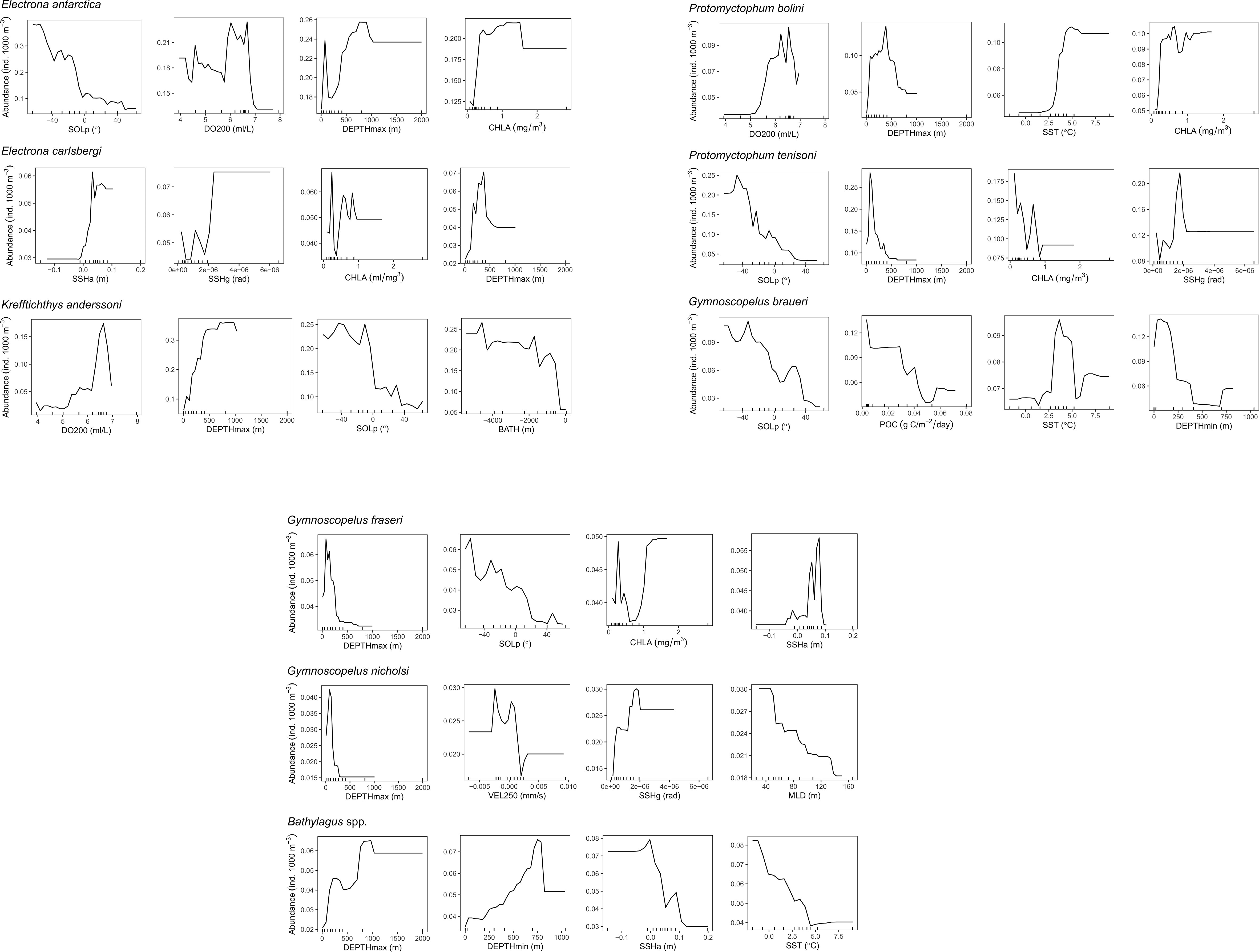
Figure 3 Partial dependence plots showing the effect of environmental covariates (horizontal axes) on the predicted abundance (vertical axes) of eight myctophid species and the genus Bathylagus, after accounting for the effects of all other variables in the boosted regression tree model. Tick marks inside the plots along the horizontal axes represent the distribution of data points used to build the model. Only the four most influential predictors for each taxonomic group are shown, ordered by level of importance from high to low. The full names and a description of all environmental covariates are given in Table 1.
Abundance predictions varied between net type (NET) and codend mesh size (CODEND) with the highest predictions for the RMT 25 with a codend mesh of 5 mm (see example Figure S5). However, different gear types produced the same patterns in relative abundance between predictions (Figure S5). Net type and codend mesh size did not fall within the top four most important covariates for any species-specific models and consistently showed the lowest relative contribution scores with an average of 1.0% and 1.9%, respectively.
3.2.1 Predictions in vertical space
The vertical distribution of all species, except for G. nicholsi, depended on SOLp (Figures 3–5); and depth preferences varied across species (Figures 3, 4). Clear day-night differences in abundance predictions were observed with higher abundances at night-time (SOLp < 0°) compared to daylight hours (SOLp > 0°). Although abundance predictions seemed to decrease later in the day (larger solar angle) for P. bolini compared to other species and abundance was relatively consistent across day and night for G. nicholsi (Figure 4). It must be noted that all species occurred in the top 200 m of the water column at night-time as depicted by the DEPTHmin covariate (Figure 5; Figure S6-S14). However, discussion of proceeding results is in relation to the DEPTHmax variable that reflects the maximum depth of capture for a species.
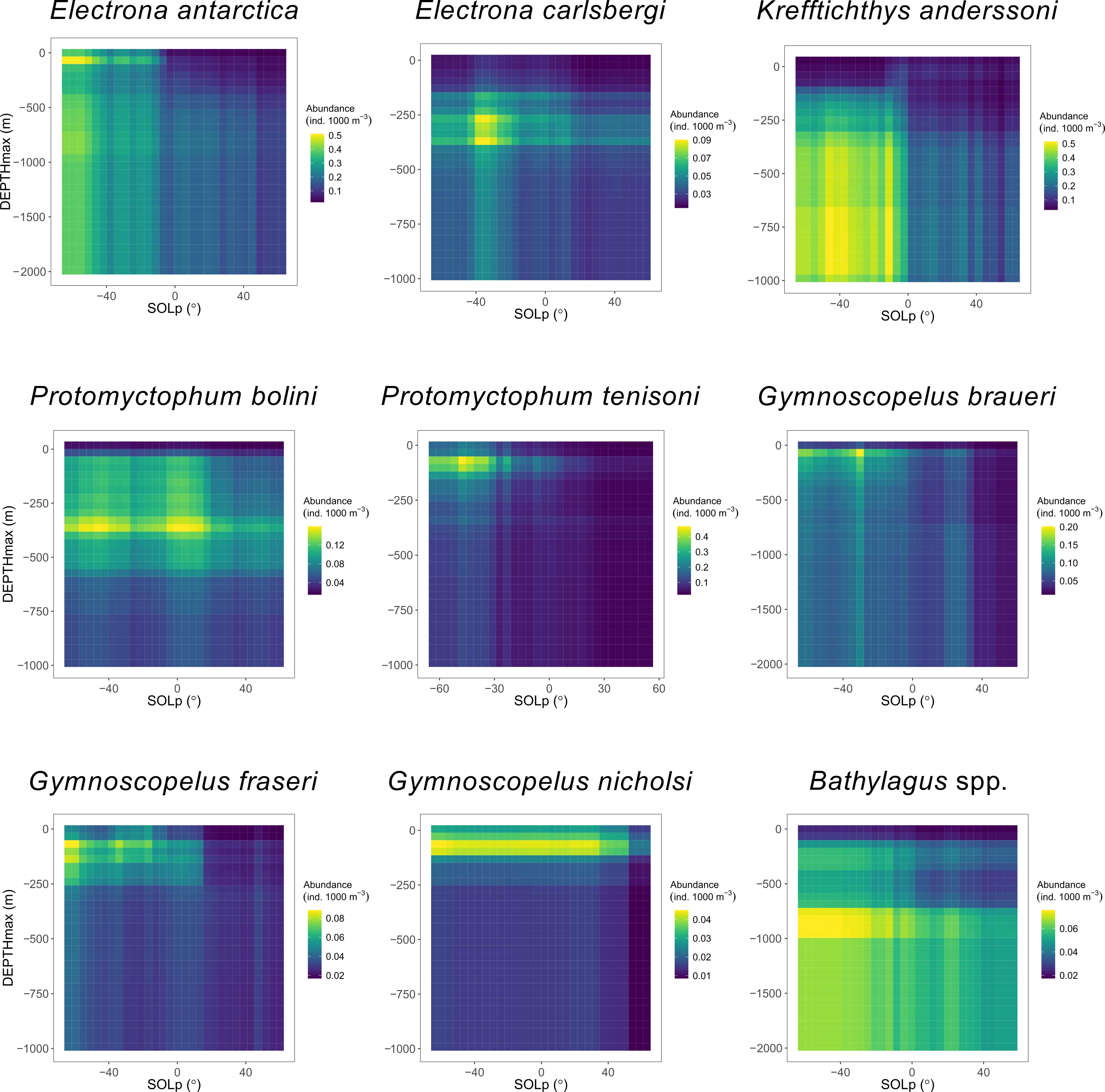
Figure 4 Predicted abundance of eight species of myctophid and the genus Bathylagus in relation to maximum depth (DEPTHmax) of the trawl, given the variation in solar position (SOLp; negative values indicate night-time, positive values indicate daytime) as predicted by species-specific boosted regression tree models. Color depicts abundance.
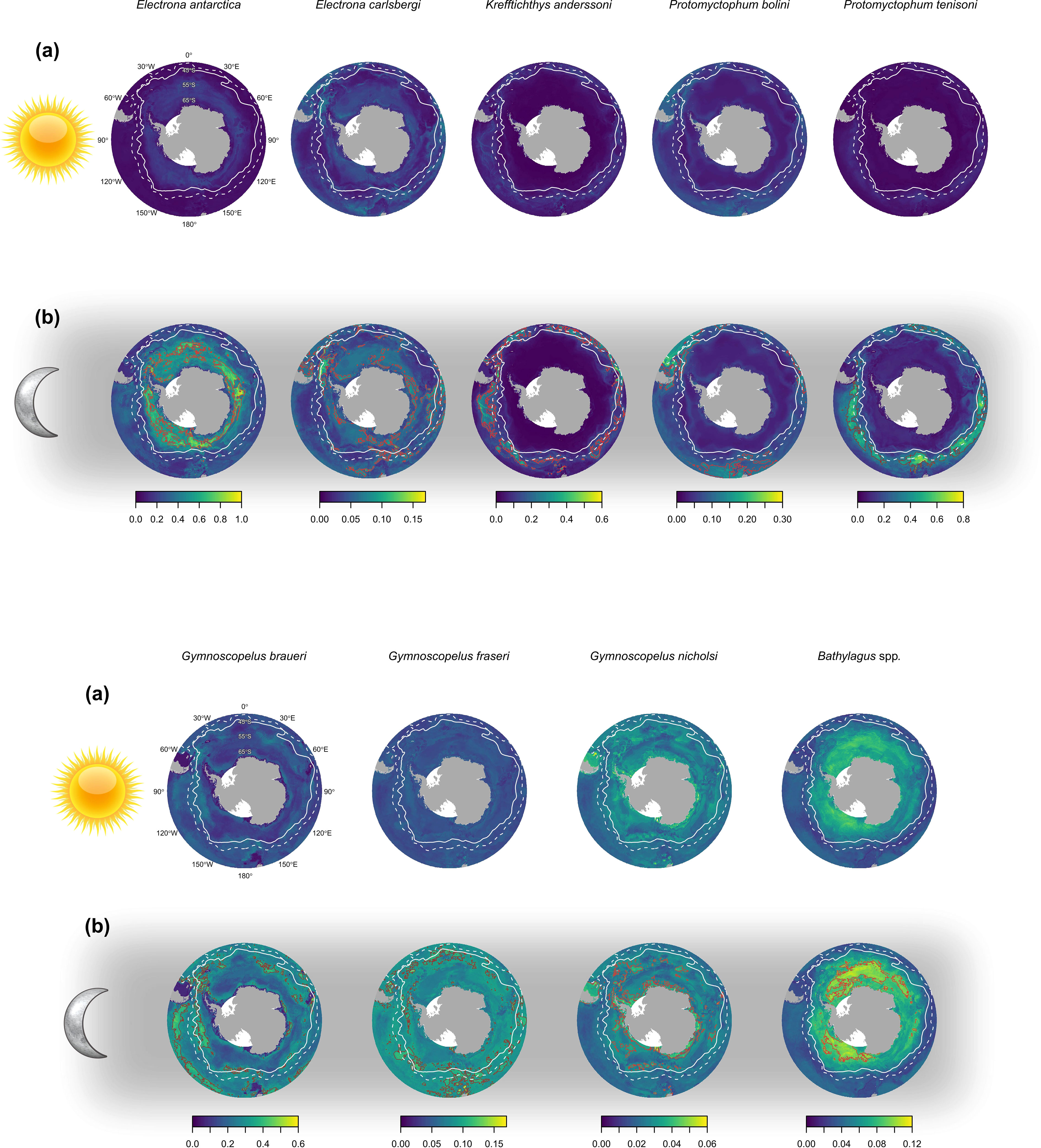
Figure 5 The predicted abundance (ind. 1000 m-3) of eight species of myctophid and the genus Bathylagus at (a) day and (b) night in the top 200 meters of the water column. The brown outline depicts the 90th percentile (top decile) that represents the most densely distributed 10% of the total abundance for the study area. The white solid line shows the position of the polar front (PF), and the white dashed line shows the position of the sub-Antarctic front (SAF). Predictions are for an RMT 25 with a codend mesh of 5 mm.
In the epipelagic zone (0 – 200 m) E. antarctica, P. tenisoni, G. braueri and G. fraseri were abundant at night (Figures 3, 4). Abundance predictions declined with depth and increasing SOLp. Electrona carlsbergi was sparse in the epipelagic (Figure 4). Predictions showed this species to be most abundant in the upper mesopelagic (200 – 400 m) at night where abundance gradually declined with increasing depth and SOLp. Krefftichthys anderssoni was less constrained by depth and predictions showed a consistent level of abundance across both the upper and lower mesopelagic (200 – 1000 m). However, this was constrained to the night-time hours as abundance predictions decreased from sunrise. Bathylagus spp. were most abundant at SOLp < 0° (i.e. night time) in the lower mesopelagic (600 to 1000 m). Abundance was predicted to reduce only marginally at depths deeper than 1000 m and during the daylight hours, showing minimal day-night differences. Bathylagus spp. were also relatively sparse at depths shallower than 600 m. Protomyctophum bolini showed highest abundances for the upper mesopelagic with their distribution extending into both the epipelagic and the lower mesopelagic. Gymnoscopelus nicholsi was most abundant in the epipelagic zone.
3.3 Spatial predictions
Abundance predictions for species groups revealed broadly circumpolar distribution patterns and clear day-night differences in the epipelagic zone (Figure 5). Predicted abundance in the epipelagic was lower during the day (Figure 5A) compared to the night (Figure 5B) for all species except for G. nicholsi.
Two taxonomic groups, E. antarctica and Bathylagus spp. showed distinct Antarctic distributions with the top decile of their predicted total abundance located south of the PF. Electrona carlsbergi showed a patchy spatial distribution with the highest densities close to the PF. Dense aggregations were predicted in areas of high productivity, for example frontal zones of the Scotia Sea, north of South Georgia, and the southern Patagonian slope spanning to the Falkland Islands. Highest abundance predictions were mainly associated with oceanic regions, except for the Argentinian slope region.
Krefftichthys anderssoni and P. tenisoni were distributed as circumpolar bands from the PF to north of the sub-Antarctic Front (SAF). The most densely distributed 10% of the total abundance for both species was centered on the SAF. The predicted distribution of both species extended as far north as 45°S off the eastern side of South America. Protomyctophum tenisoni appeared to be less common in the eastern sector of the Southern Ocean (from 0° to 90°E), while high abundance estimates were shown for K. anderssoni north of the Kerguelen Islands congruent with the SAF. Protomyctophum bolini abundance was sparsely distributed south of the PF, but it was densely distributed north of the SAF. The top decile of their predicted total abundance appeared to be constrained to three different regions: the southern Argentinian slope to the Falkland Islands and north of South Georgia, within the frontal zones to the north of the Kerguelen Islands, and in the region of the Campbell plateau south of New Zealand.
Gymnoscopelus braueri and G. fraseri showed a spatially broad and patchy circumpolar distribution from the Antarctic continent to 45°S. However, abundance predictions suggested an oceanic distribution for G. braueri with the highest densities associated with the sub-Antarctic, Polar Frontal and Antarctic zones. In contrast, high abundance areas for G. fraseri appeared to be associated with the slope waters around Falkland Islands, South Georgia, the Kerguelen Islands and south of New Zealand as well as the oceanic regions of frontal zones. Gymnoscopelus nicholsi showed a similarly patchy circumpolar distribution, however, distribution patterns were broadly Antarctic with highest densities predominantly south of the PF. The highest abundances were associated with the Antarctic continental shelf, Argentinian slope waters and the Kerguelen Islands, as well as the oceanic regions of the Antarctic zone.
Species were categorized into three broad groupings based on abundance predictions (Figure 6). We used the categories proposed by McGinnis (1982): “Antarctic”, “Broadly Antarctic”, and “sub-Antarctic”. Most of our study species were categorized as “Broadly Antarctic” (E. carlsbergi, K. anderssoni, P. tenisoni, G. nicholsi and G. braueri), while E. antarctica and Bathylagus spp. were classified as “Antarctic” and only one species was considered sub-Antarctic (P. bolini). We did not categorize G. fraseri as clear patterns in their distribution were difficult to distinguish.
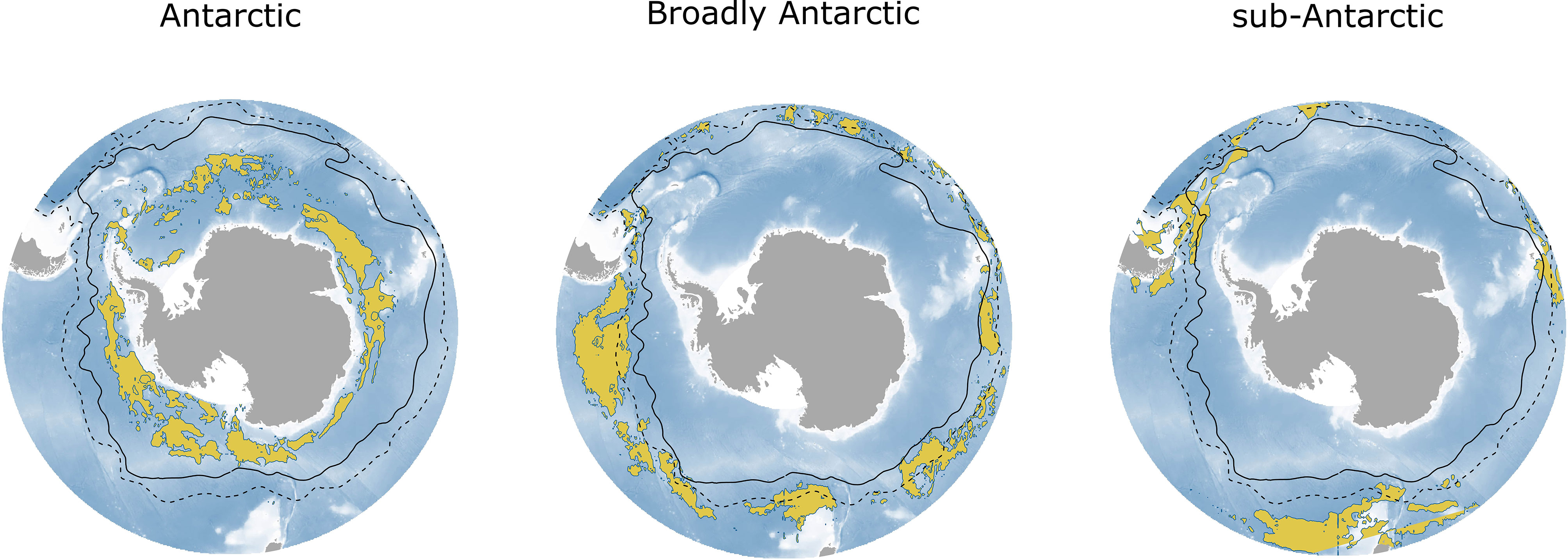
Figure 6 The total combined night-time abundance by the broad groupings: ‘Antarctic’, ‘Broadly Antarctic’ and ‘sub-Antarctic’. Abundance is shown in yellow as the 90th percentile (top decile) of the predicted abundance across the Southern Ocean. The ‘Antarctic’ grouping includes Bathylagus spp. and E. antarctica; ‘Broadly Antarctic’ includes E. carlsbergi, K. anderssoni, P. tenisoni, G. nicholsi and G. braueri; and ‘sub-Antarctic’ includes P. bolini only. The black solid line shows the position of the polar front (PF), and the black dashed line shows the position of the sub-Antarctic front (SAF).
4 Discussion
This study provides the first circumpolar predictions of the abundance of eight myctophid species and the genus Bathylagus. We used data from Myctobase, a database of survey data of mesopelagic fishes, which integrates and standardizes disparate biodiversity data. Boosted regression trees allowed us to examine the environmental, vertical, and geographic patterns of abundance. The novel findings from this study demonstrate the power of a collaborative database and modelling framework approach for dealing with data from heterogenous sources adding information value to existing data. This approach can be used to examine patterns in the circumpolar distribution of myctophid abundance building upon existing modelling efforts that have previously used presence-absence or presence only data. By examining patterns in abundance, we were able to highlight important geographic areas of mesopelagic fish occurrence.
4.1 Environmental predictors
The relative importance of selected environmental variables suggests some of the factors that influence the patterns of abundance of our study species. Depth and solar position were consistently important and interacting predictors of abundance. This result is not unexpected given that many mesopelagic fish species undertake diel vertical migration (Duhamel et al., 2000; Collins et al., 2008; Van de Putte et al., 2010; Collins et al., 2012; Saunders et al., 2015; Lourenco et al., 2017). The predominant driving factors of diel vertical migration include the physiological requirement to feed on high concentrations of zooplankton in the epipelagic and to avoid visual predators by migrating to depths during the day (Catul et al., 2011). However, the depth distributions of our study species may be confounded by the daytime net avoidance behaviors of mesopelagic fishes (Collins et al., 2008; Fielding et al., 2012), which might explain the higher abundances at night compared to day (e.g. Figure 4). Studies conducting daytime trawls on acoustically detected fish in the epipelagic have failed to catch aggregations whilst night-time trawls consistently yield higher catch rates, suggesting that fish are avoiding the trawl net (Collins et al., 2008; Collins et al., 2012). In this study, the depth distribution and day-night differences in abundance were likely the result of both diel vertical migration and net avoidance.
Maximum migration depth has been linked to dissolved oxygen levels, with the depth of migration shallower in regions with low oxygen levels at the subsurface (Bianchi et al., 2013; Klevjer et al., 2016). A suggested hypothesis for the link between migration depth and dissolved oxygen is that individuals need only travel as far as the oxygen minimum zone to use this region as a refuge from visual predators who generally have higher oxygen demands (Song et al., 2022). We suggest that the high relative importance of DO200 for predicting abundance of E. antarctica, P. bolini and K. anderssoni might be a consequence of these species utilizing oxygen minimum zones as a predator avoidance strategy. Alternatively, studies on Benthosema glaciale in the Boreal to Arctic northeast Atlantic show that the latitudinal variation in seasonal light regime may also be an important control of mesopelagic fish depth distribution patterns (Langbehn et al., 2019; Langbehn et al., 2022), highlighting the need for further investigations into the environmental drivers of myctophid vertical migration behavior in the Southern Ocean.
Chlorophyll-a (CHLA) concentration is a proxy for phytoplankton biomass indicating regions of nutrient rich water (Sokolov and Rintoul, 2007b) and potentially profitable foraging areas (Bost et al., 2009; Block et al., 2011). We found that CHLA concentration was important for some species, however the response curves between abundance and CHLA were complex. There might be a temporal or spatial lag between increased CHLA concentration and increasing fish abundance due to the temporal separation of primary and secondary production (Loots et al., 2007; Lehodey et al., 2010). Previous studies have shown similarly mixed results with negative relationships found for E. antarctica abundance and CHLA concentration at Kerguelen Islands (Loots et al., 2007), and the absence of a relationship between mesopelagic fish biomass and CHLA in the northeast Pacific Ocean (Saijo et al., 2017). Our results and those from previous studies suggest a decoupling in time and space between CHLA concentration and mesopelagic fish abundance.
Prey availability is likely to be a strong determinant of mesopelagic fish distribution. Direct measurements of prey availability across large spatial extents are difficult to obtain, so researchers typically rely on remotely sensed or modelled products that are linked to prey availability. We used particulate organic carbon (POC) as a proxy for prey availability, which was calculated from the seasonal variation index of net primary production monthly layers (Table 1). Ecological theory states that primary production constrains biomass at higher trophic levels (Jennings et al., 2008). Additionally, mesopelagic fish biomass has been linked to primary production (Irigoien et al., 2014; Proud et al., 2017). However, in this study POC was important for only one species, G. braueri. Ultimately, pelagic food webs are fuelled by the primary production produced in the epipelagic zones of the world’s ocean (Choy et al., 2017). Here, the biomass generated in the form of zooplankton and filter feeding gelatinous organisms is consumed by a range of taxa including mesopelagic fishes (Choy et al., 2017; Drazen and Sutton, 2017). Production is transported vertically by migratory species or sinking particles, partitioning energy across large depth gradients (Choy et al., 2015). Further, movement of organisms among habitats such as higher predators or expatriate populations can introduce new production and pathways for energy transfer enhancing local production (Polis et al., 1997; Trebilco et al., 2016). Clearly, pelagic food web dynamics are complex, and the lack of clear relationships in this study might be due to the mesopelagic fish assemblage being subsidized by production outside of what is captured by POC measurements.
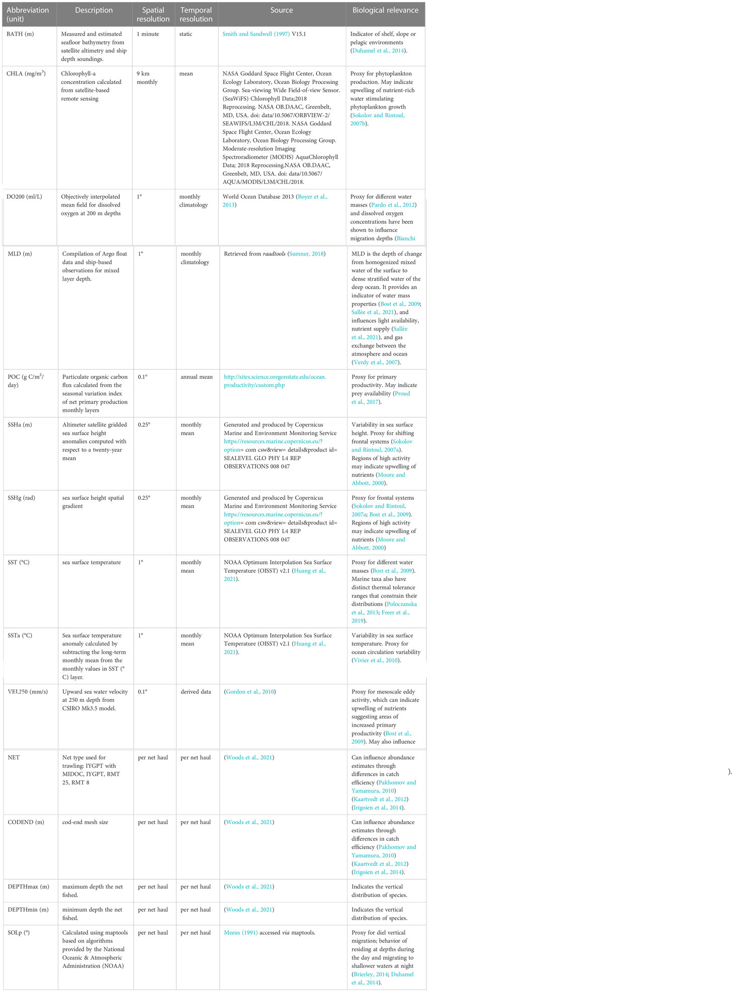
Table 1 Environmental covariates used to model the abundance of a selection of mesopelagic fish species in the Southern Ocean.
In ectotherms, metabolism is temperature dependent, which affects physiological functions such as growth and reproduction of marine organisms (Gillooly et al., 2001; Clarke, 2009). Mesopelagic fish species have a range of thermal tolerances with some having a narrower range than others (Freer et al., 2019). In this study, we suggest that SST was a proxy for this tolerance range as all species in this study either migrate to surface waters at night or inhabit near-surface waters as larvae or juveniles (Lancraft et al., 1989; Duhamel et al., 2000; Pusch et al., 2004; Collins et al., 2012). In this study G. braueri showed a narrower optimal temperature range compared to that of P. bolini, which agrees with predicted future distributions of myctophids (Freer et al., 2019). Freer et al. (2019) showed that G. braueri was predicted to lose suitable habitat under different climate change scenarios given its narrow thermal tolerance, while conversely, P. bolini was predicted to fair better as it had a wider thermal range.
Other important predictors included VEL250, SSHg and SSHa, which indicate ocean fronts and eddies. Regions of high water velocity increases the availability of nutrients fuelling marine food webs (Moore and Abbott, 2000). The increase in nutrients promotes increased productivity and zooplankton biomass (Bost et al., 2009) and areas of upwelling and downwelling help to aggregate prey. Myctophid fish concentrate along the periphery of anti-cyclonic eddies where other prey species aggregate (Pakhomov and Froneman, 2000). Additionally, abundance at Antarctic latitudes is driven by oceanic processes, such as high intensity eddies, which facilitate expatriation of mesopelagic fish (Langbehn et al., 2022), for example this has been shown to occur in the Scotia Sea (Saunders et al., 2017; Murphy et al., 2021).
Variability in abundance predictions between net type and codend mesh size aligns with previous research, which demonstrates differences in catch efficiency between net types (Pakhomov and Yamamura, 2010; Kaartvedt et al., 2012). However, we note the minimal influence of net type and codend mesh size on the explanatory power of the final models, which suggests that other environmental variables were more important in predicting abundance.
4.1.1 Vertical distribution
Patterns in the vertical distribution of mesopelagic fish exhibited clear diurnal differences in abundance for all species except for G. nicholsi. The night-time vertical habitat trends broadly followed that of previous research (Duhamel et al., 2000; Collins et al., 2008; Hulley and Duhamel, 2011; Saunders et al., 2015; Lourenco et al., 2017; Moteki et al., 2017). The epipelagic zone (0 – 200 m) was important night-time habitat for E. antarctica, P. tenisoni, G. braueri and G. fraseri, which follows their reported distribution in the Kerguelen region (Duhamel et al., 2000; Hulley and Duhamel, 2011), the Scotia Sea (Collins et al., 2008; Saunders et al., 2015), and off Wilkes Land, East Antarctica (Moteki et al., 2017). Deeper in the water column, E. carlsbergi, K. anderssoni and P. bolini showed highest night-time abundances within the upper mesopelagic zone (200 – 400 m) consistent with observations from the Kerguelen region (Duhamel et al., 2000) and the Scotia Sea (Collins et al., 2008; Lourenco et al., 2017). High night-time abundance for K. anderssoni extended beyond the upper mesopelagic to depths of 1000 m. Previous research has shown an increase in size of individuals with depth suggesting ontogenetic descent (Lourenco et al., 2017), which may reflect the presence of adults within the data we analyzed here. Typically, Bathylagus spp. are deep-sea species dominating the lower mesopelagic zone and are thought to undertake DVM (Lancraft et al., 1989; Koubbi et al., 2011a; Collins et al., 2012), which was reflected in this study. The observed reduced abundance for species during the day provided evidence of DVM consistent with previous reports (Duhamel et al., 2000; Collins et al., 2008; Van de Putte et al., 2010; Collins et al., 2012; Saunders et al., 2015; Lourenco et al., 2017), this is difficult to disentangle from net avoidance behaviors as we described earlier.
We found minimal day-night differences in abundance for G. nicholsi. Previously, G. nicholsi have been sampled across all three depth zones (epipelagic, upper, and lower mesopelagic) with the highest abundance observed in the top 200 m at night with evidence of DVM (Duhamel et al., 2000; Pusch et al., 2004; Collins et al., 2008; Saunders et al., 2015). In our study the depth range of G. nicholsi appeared to be limited to the epipelagic zone with no evidence of DVM.
Overall, our findings provide evidence for non-synchronous DVM patterns for some species. The presence of individuals over broad depth ranges at night-time, for example E. antarctica and K. anderssoni, could suggest foray-type behaviors among myctophids. Studies in the Scotia Sea have similarly demonstrated the presence of myctophid species at depth during the night (Collins et al., 2008; Saunders et al., 2014). Discrepancies between our findings and those of other studies may be linked to the spatially and temporally dynamic nature of the DVM habits of fish. DVM can vary with season (Saunders et al., 2015; Langbehn et al., 2019; Langbehn et al., 2022) and latitude (Proud et al., 2017; Langbehn et al., 2019; Langbehn et al., 2022), for example, during the summer months at high latitudes the longer daylight hours confine mesopelagic fish to greater depths to avoid predators, leading to a decline in vertical migration amplitude (Langbehn et al., 2019; Langbehn et al., 2022). Further, DVM behaviors can vary depending on the life stage of some species (Collins et al., 2008; Moteki et al., 2009; Lourenco et al., 2017). Survey data of mesopelagic fishes are sparse and highly heterogenous in space and time (Lehodey et al., 2010). The abundance data we had access to for these species may be inadequate to truly represent the nuanced nature of their DVM behaviors. For example, observations may not be representative of the life stages that exhibit DVM, possibly a consequence of the selectivity differences of trawl nets (Pakhomov and Yamamura, 2010; Kaartvedt et al., 2012). Accurately capturing the subtleties of DVM behavior would require repeated sampling to depict temporal dynamics and expanding the spatial extent and vertical resolution of sampling for broader geographical coverage.
4.2 Geographic distribution
We draw comparisons with habitat modelling studies that have used a range of modelling algorithms and data types at both regional and circumpolar scales (Loots et al., 2007; Hulley and Duhamel, 2011; Koubbi et al., 2011b; Flynn and Williams, 2012; Duhamel et al., 2014; Freer et al., 2019; Freer et al., 2020). In most instances our estimated regions of high abundances aligned with previous circumpolar habitat modelling studies (Duhamel et al., 2014; Freer et al., 2019). These studies used ensemble approaches with presence-only data, or presence-absence data, which provides a species’ probability of presence mapped to a geographic area giving an indication of suitable habitat. The relationship between a species presence and its abundance varies spatially, temporally and by species (Karlson et al., 2011; Johnston et al., 2015). Thus, a high probability of occurrence in a location might not always equate to a high abundance and may not effectively capture the core habitat of a species (Renwick et al., 2012; Johnston et al., 2015). The differences between our model predictions and those from the studies described may be explained by the different types of output information and differences in the spatial extent of datasets resulting from variability in modelling approaches.
Species distributions of mesopelagic fish have been categorized into the three broad groupings proposed by McGinnis (1982): “Antarctic”, “Broadly Antarctic”, and “sub-Antarctic” (Duhamel et al., 2014; Freer et al., 2020). In this study, E. antarctica showed an “Antarctic” distribution in agreement with circumpolar occurrence models (Duhamel et al., 2014; Freer et al., 2019; Freer et al., 2020) and abundance models at the Kerguelen Plateau (Loots et al., 2007). Bathylagus spp. were similarly “Antarctic” in their distribution. In the Southern Ocean, there are five known species, two of which match this distributional range, Bathylagus antarcticus (Gon and Heemstra, 1990; Moteki et al., 2009; Collins et al., 2012) and Bathylagus niger (Gon and Heemstra, 1990; Kobylianskii, 2006). Put together with our vertical distribution findings for Bathylagus spp. this may indicate that most of the individuals here were that of B. antarcticus and B. niger.
Krefftichthys anderssoni, and P. tenisoni were “Broadly Antarctic” in their distribution, again in agreement with occurrence models (Duhamel et al., 2014; Freer et al., 2020); and models of biomass at Macquarie Island (Flynn and Williams, 2012). Protomyctophum bolini showed a more northerly distribution compared to previous habitat models suggesting a “sub-Antarctic” distribution pattern. Models based on occurrence data have described their distribution as “broadly Antarctic”, ranging from the SACCF to the SAF (Duhamel et al., 2014; Freer et al., 2020). However, in this study, the core abundance for this species was located north of the SAF in three localized and highly productive regions (Moore and Abbott, 2000). Our findings agree with previous research showing core reproductive populations for P. bolini along with other myctophid species are centered at sub-Antarctic latitude (Saunders et al., 2017).
Gymnoscopelus nicholsi has been described as “broadly Antarctic” with an affinity for shelf and slope areas (Duhamel et al., 2014; Freer et al., 2020). Adults are benthopelagic and are typically distributed close to the seabed over the Argentinian slope, the Crozet slope, South Georgia slope and the Kerguelen Plateau (Linkowski, 1985). Larvae and juveniles are generally located in pelagic waters shallower in the water column (Linkowski, 1985). This may explain our abundance predictions across a diverse range of habitat types.
Predictions for E. carlsbergi show patterns of high abundance extending from the SAF to the continent suggesting a “broadly Antarctic” distribution. Freer et al. (2020) found high habitat suitability north of the PF at depths of 500 – 1000 m and high habitat suitability south of the PF at shallower depths (0 – 200 m) with 3D species distribution models. This pattern of deeper residency at lower latitude was first hypothesized by (Hulley, 1981). This corroborates our findings of regions of high abundance south of the PF in the epipelagic zone.
High abundance regions for G. braueri were predominately located near the PF. Previous habitat modelling studies have predicted suitable habitat in restricted regions south of the PF (Freer et al., 2020). High abundances have also been recorded at the South Orkneys and South Shetland Islands (Pusch et al., 2004; Saunders et al., 2015); and in the Polar Frontal Zone of the Scotia Sea (Saunders et al., 2015). However, this species has been documented north of the PF at Ridge Gap, Macquarie Island (Flynn and Williams, 2012). Our results match with the “broadly Antarctic” distribution suggested in Duhamel et al. (2014), rather than “Antarctic” as indicated by Freer et al. (2020).
Abundance predictions for G. fraseri were dispersed across the study area from 45°S to the Antarctic continent. Clear patterns in their distribution were difficult to distinguish from our predictions. Gymnoscopelus fraseri have previously been recorded between the SACCF and the PF (Collins et al., 2012; Saunders et al., 2015). Suitable habitat has also been predicted as far north as the SAF (Duhamel et al., 2014). The discrepancy between our study and observed distributions may be explained by the relatively poor performance of this model.
4.3 Developing ecological perspectives
Patterns in myctophid abundance are influenced by meso- and sub-mesoscale oceanographic features where the Polar Front acts as a major delimiting feature for community composition. The Polar Front is one of the most important oceanic fronts in delineating ecological communities in the Southern Ocean (Grant et al., 2006; Longhurst, 2007; Koubbi et al., 2011b; De Broyer et al., 2014). Southern Ocean marine ecosystems are heavily influenced by frontal systems that separate regions with distinct physical and chemical properties (Grant et al., 2006; Longhurst, 2007). The varying physical and chemical properties are important determinants of regional food web structure and function (Murphy et al., 2012). In our study the Polar Front marked a clear transition from a diverse mesopelagic fish community in the sub-Antarctic zone to a less diverse community south of the Polar Front in the Antarctic zone. Previous studies have demonstrated latitudinal variability in food web structure as indicated by the presence of longer food chains in the north (Stowasser et al., 2012; Ward et al., 2012; Saporiti et al., 2015; Woods et al., 2020). The increase in food chain length from south to north is accompanied by an increase in species richness (Koubbi et al., 2011b; Ward et al., 2012; Saporiti et al., 2015). Food chain theory dictates that food chain length increases with increasing ecosystem size and species richness (Cohen and Newman, 1991; Post et al., 2000; Post, 2002). In our study the contrasting patterns in community composition with higher species diversity north of the Polar Front may be indicative of latitudinal variability in food web structure.
Southern Ocean ecosystems are additionally characterized by a high degree of ecological connectivity between regions due to cross-frontal processes such as surface currents and eddy activity (Hunt et al., 2016; Murphy et al., 2021). Many myctophid species, such as E. carlsbergi, P. bolini, P. tenisoni, G. braueri, G. fraseri and G. nicholsi, found south of the Polar Front do not recruit locally and are thought to be of sub-Antarctic origin (Saunders et al., 2017). Spawning and recruitment is suggested to occur in waters north of the Polar Front and high-intensity eddies facilitate the movement of adults into Antarctic waters (Saunders et al., 2017). The mesopelagic fish biomass north of the Polar Front is likely to be of crucial importance to sustaining mesopelagic fish biomass at Antarctic latitudes (Murphy et al., 2013; Saunders et al., 2017). This means that expatriate populations may play a key role in the maintenance of ecosystem stability and sustaining higher-level predator biomass at Antarctic latitudes. Habitat modelling studies do not currently consider the extent that expatriation plays in determining habitat range. Future ecological studies are needed to resolve important areas for reproduction, migration pathways and connectivity processes.
4.4 Conclusion
We used data from Myctobase to model patterns in abundance of key mesopelagic fish taxa in the Southern Ocean. Data originated from multiple research cruises, each employing a specific sampling strategy. We accounted for the complexity and uncertainty in the data by explicitly modelling aspects of the survey methodology, providing an example of data usage from Myctobase. We demonstrate the value of net data to resolve patterns in relative abundance of species, providing a complementary approach to acoustic methods. Detailed knowledge of the environmental and latitudinal preferences of mesopelagic fishes is imperative to understand how the community may respond to future environmental change in the Southern Ocean. Our findings suggest that abundance could be influenced by meso- and sub-mesoscale oceanographic features where the Polar Front is a major delimiting feature for the distribution of species. Although finer resolution data are needed to test this hypothesis further. Specific environmental and latitudinal preferences will likely influence the vulnerability of certain species to shifting environmental conditions. For example, G. braueri showed a narrow optimal temperature range suggesting this species is likely to be vulnerable to ocean warming in the future, which corroborates findings by Freer et al. (2019). Further, a shift in frontal features may disrupt the influx of expatriate fish to Antarctic latitudes, leading to localized population depletion and a decrease in prey availability for predators. Our study highlights remaining uncertainties such as mesopelagic fish habitat in the Pacific sector. We found regions of high abundance for some species in the Ross, Bellingshausen, and Amundsen Seas despite this being a data poor region. Subsequently, this area would benefit from increased sampling effort. Our spatial analysis is an important step toward resolving important habitat of mesopelagic fishes, which underpins knowledge of shifting food web dynamics into the future. Future modelling efforts should investigate the use of more direct indicators of prey availability by including data layers such as those from the spatial ecosystem and population dynamics model or SEAPODYM (Lehodey et al., 2008). Continued contributions to Myctobase will allow improvement of the models we created here and establishment of a solid foundation upon which to understand future population change.
4.4.1 Permission to reuse and copyright
Figures, tables, and images will be published under a Creative Commons CC-BY license and permission must be obtained for use of copyrighted material from other sources (including re-published/adapted/modified/partial figures and images from the internet).It is the responsibility of the authors to acquire the licenses, to follow any citation instructions requested by third-party rights holders, and cover any supplementary charges.). It is the responsibility of the authors to acquire the licenses, to follow any citation instructions requested by third-party rights holders, and cover any supplementary charges.
Data availability statement
Publicly available datasets were analysed in this study. This data can be found on Zenodo: https://zenodo.org/record/6809070, GBIF: https://doi.org/10.15468/u25dy5, OBIS https://obis.org/dataset/d8b738c8-6eda-4735-8136-53630eedab6a and the SCAR Antarctic biodiversity Portal https://ipt.biodiversity.aq/resource?r=myctobase&v=1.0. The R code used in this paper can be found on GitHub: https://github.com/BreeWoods/Myctobase-SDMs.
Author contributions
BW led the project. BW, AVP, RT, and AW were responsible for the conceptualization and design of the project. All authors contributed to the data analysis. All authors contributed to the writing and editing of this manuscript and approved the submitted version.
Funding
We thank the following organizations for providing financial support: The Belgian Science Policy Office (BELSPO, contract n°FR/36/AN1/AntaBIS) in the Framework of EU-Lifewatch, The Australian Research Council’s Special Research Initiative for Antarctic Gateway Partnership, The Institute for Marine and Antarctic Studies, The Bottom of the Earth Society and the MESOPP project.
Acknowledgments
We thank and acknowledge all researchers and their institutions for contributing data to Myctobase. Thanks to Simon Wotherspoon (the Australian Antarctic Division) for his statistical advice and Mike Sumner for R support (the Australian Antarctic Division). Thanks to Sophie Bestley for providing custom code for calculating day/night periods (Institute for Marine and Antarctic Studies).
Conflict of interest
The authors declare that the research was conducted in the absence of any commercial or financial relationships that could be construed as a potential conflict of interest.
Publisher’s note
All claims expressed in this article are solely those of the authors and do not necessarily represent those of their affiliated organizations, or those of the publisher, the editors and the reviewers. Any product that may be evaluated in this article, or claim that may be made by its manufacturer, is not guaranteed or endorsed by the publisher.
Supplementary material
The Supplementary Material for this article can be found online at: https://www.frontiersin.org/articles/10.3389/fmars.2022.981434/full#supplementary-material
References
Anderson T. R., Martin A. P., Lampitt R. S., Trueman C. N., Henson S. A., Mayor D. J. (2018). Quantifying carbon fluxes from primary production to mesopelagic fish using a simple food web model. Ices. J. Mar. Sci. 76, 690–701. doi: 10.1093/icesjms/fsx234
Benoit-Bird K. J., Lawson G. L. (2016). “Ecological insights from pelagic habitats acquired using active acoustic techniques,” in Annual review of marine science, vol 8. Eds. Carlson C. A., Giovannoni S. J. (Palo Alto: Annual Reviews), 463–490. doi: 10.1146/annurev-marine-122414-034001
Bianchi D., Galbraith E. D., Carozza D. A., Mislan K. A., Stock C. A. (2013). Intensification of open-ocean oxygen depletion by vertically migrating animals. Nat. Geosci. 6, 545–548. doi: 10.1038/ngeo1837
Bivand R., Lewin-Koh N., Pebesma E., Archer E., Baddeley A., Bearman N., et al. (2021). Maptools: Tools for handling spatial objects. r package version 1.1-1.
Block B. A., Jonsen I. D., Jorgensen S. J., Winship A. J., Shaffer S. A., Bograd S. J., et al. (2011). Tracking apex marine predator movements in a dynamic ocean. Nature 475, 86–90doi: 10.1038/nature10082
Bost C. A., Cotte C., Bailleul F., Cherel Y., Charrassin J. B., Guinet C., et al. (2009). The importance of oceanographic fronts to marine birds and mammals of the southern oceans. J. Mar. Syst. 78, 363–376. doi: 10.1016/j.jmarsys.2008.11.022
Boyer T. P., Antonov J. I., Baranova O. K., Coleman C., Garcia H. E., Grodsky A., et al. (2013). World ocean database 2013. ( Silver Spring, MD, National Oceanographic Data Center) doi: 10.7289/V5NZ85MT
Brierley A. S. (2014). Diel vertical migration. Curr. Biol. 24, R1074–R1076. doi: 10.1016/j.cub.2014.08.054
Caccavo J. A., Christiansen H., Constable A. J., Ghigliotti L., Trebilco R., Brooks C. M., et al. (2021). Productivity and change in fish and squid in the southern ocean. Front. Ecol. Evol. 9. doi: 10.3389/fevo.2021.624918
Catul V., Gauns M., Karuppasamy P. K. (2011). A review on mesopelagic fishes belonging to family myctophidae. Reviews in Fish Biology and Fisheries 21, 339–354. doi: 10.1007/s11160-010-9176-4
Cherel Y., Bocher P., Trouvé C., Weimerskirch H. (2002). Diet and feeding ecology of blue petrels halobaena caerulea at iles kerguelen, southern Indian ocean. Mar. Ecol. Prog. Ser. 228, 283–299. doi: 10.3354/meps228283
Choy C. A., Haddock S. H. D., Robison B. H. (2017). Deep pelagic food web structure as revealed by in situ feeding observations. Proc. R. Soc. B-Biol. Sci. 284, 10. doi: 10.1098/rspb.2017.2116
Choy C. A., Popp B. N., Hannides C. C. S., Drazen J. C. (2015). Trophic structure and food resources of epipelagic and mesopelagic fishes in the north pacific subtropical gyre ecosystem inferred from nitrogen isotopic compositions. Limnol. Oceanogr. 60, 1156–1171. doi: 10.1002/lno.10085
Cisewski B., Hátún H., Kristiansen I., Hansen B., Larsen K. M. H., Eliasen S. K., et al. (2021). Vertical migration of pelagic and mesopelagic scatterers from ADCP backscatter data in the southern Norwegian Sea. Front. Mar. Sci. 7. doi: 10.3389/fmars.2020.542386
Clarke A. (2009). “Temperature and marine macroecology,” in Marine macroecology. Eds. Witman J. D., Roy K. (Chicago, IL: The University of Chicago Press), 251–278.
Clarke L. J., Trebilco R., Walters A., Polanowski A. M., Deagle B. E. (2020). DNA-Based diet analysis of mesopelagic fish from the southern kerguelen axis. Deep-Sea. Res. Part II.: Topical. Stud. Oceanogr. 174, 104494. doi: 10.1016/j.dsr2.2018.09.001
Clements C. F., Blanchard J. L., Nash K. L., Hindell M. A., Ozgul A. (2017). Body size shifts and early warning signals precede the historic collapse of whale stocks. Nat. Ecol. Evol. 1. doi: 10.1038/s41559-017-0188
Cohen J. E., Newman C. M. (1991). Community area and food-chain length: theoretical predictions. Am. Nat. 138, 1542–1554. doi: 10.1086/285299
Collins M. A., Ross K. A., Belchier M., Reid K. (2007). Distribution and diet of juvenile patagonian toothfish on the south Georgia and shag rocks shelves (Southern ocean). Mar. Biol. 152, 135–147. doi: 10.1007/s00227-007-0667-3
Collins M. A., Stowasser G., Fielding S., Shreeve R., Xavier J. C., Venables H. J., et al. (2012). Latitudinal and bathymetric patterns in the distribution and abundance of mesopelagic fish in the Scotia Sea. Deep-Sea. Res. Part II-Topical. Stud. Oceanogr. 59, 189–198. doi: 10.1016/j.dsr2.2011.07.003
Collins M. A., Xavier J. C., Johnston N. M., North A. W., Enderlein P., Tarling G. A., et al. (2008). Patterns in the distribution of myctophid fish in the northern Scotia Sea ecosystem. Polar. Biol. 31, 837–851. doi: 10.1007/s00300-008-0423-2
Constable A. J., Melbourne-Thomas J., Corney S. P., Arrigo K. R., Barbraud C., Barnes D. K. A., et al. (2014). Climate change and southern ocean ecosystems I: how changes in physical habitats directly affect marine biota. Global Change Biol. 20, 3004–3025. doi: 10.1111/gcb.12623
Crase B., Liedloff A. C., Wintle B. A. (2012). A new method for dealing with residual spatial autocorrelation in species distribution models. Ecography 35, 879–888. doi: 10.1111/j.1600-0587.2011.07138.x
Davison P., Lara-Lopez A., Anthony Koslow J. (2015). Mesopelagic fish biomass in the southern California current ecosystem. Deep-Sea. Res. Part II.: Topical. Stud. Oceanogr. 112, 129–142. doi: 10.1016/j.dsr2.2014.10.007
De Broyer C., Koubbi P., Griffiths H., Grant S. A. (2014). Biogeographic atlas of the southern ocean (Cambridge: Scientific Committee on Antarctic Research Cambridge, UK).
Dornan T., Fielding S., Saunders R. A., Genner M. J. (2019). Swimbladder morphology masks southern ocean mesopelagic fish biomass. Proc. R. Soc. B-Biol. Sci. 286, 8. doi: 10.1098/rspb.2019.0353
Dornan T., Fielding S., Saunders R. A., Genner M. J. (2022). Large Mesopelagic fish biomass in the southern ocean resolved by acoustic properties. Proc. R. Soc. B.: Biol. Sci. 289, 20211781. doi: 10.1098/rspb.2021.1781
Drazen J. C., Sutton T. T. (2017). Dining in the deep: The feeding ecology of deep-Sea fishes. Annu. Rev. Mar. Sci. 9, 337–366. doi: 10.1146/annurev-marine-010816-060543
Duan N. (1983). Smearing estimate: A nonparametric retransformation method. J. Am. Stat. Assoc. 78, 605–610. doi: 10.2307/2288126
Duhamel G., Hulley P. A., Causse R., Koubbi P., Vacchi M., Pruvost P., et al. (2014). “Biogeographic patterns of fish,” in Biogeographic atlas of the southern ocean (Cambridge, UK: Scientific Committee of Antarctic Research), 328–362.
Duhamel G., Koubbi P., Ravier C. (2000). Day and night mesopelagic fish assemblages off the kerguelen islands (Southern ocean). Polar. Biol. 23, 106–112. doi: 10.1007/s003000050015
Elith J., Graham C. H., Anderson R. P., Dudik M., Ferrier S., Guisan A., et al. (2006). Novel methods improve prediction of species’ distributions from occurrence data. Ecography 29, 129–151. doi: 10.1111/j.2006.0906-7590.04596.x
Elith J., Leathwick J. R., Hastie T. (2008). A working guide to boosted regression trees. J. Anim. Ecol. 77, 802–813. doi: 10.1111/j.1365-2656.2008.01390.x
Escobar-Flores P. C., O’Driscoll R. L., Montgomery J. C. (2018). Spatial and temporal distribution patterns of acoustic backscatter in the new Zealand sector of the southern ocean. Mar. Ecol. Prog. Ser. 592, 19–35. doi: 10.3354/meps12489
Fielding S., Watkins J. L., Collins M. A., Enderlein P., Venables H. J. (2012). Acoustic determination of the distribution of fish and krill across the Scotia Sea in spring 2006, summer 2008 and autumn 2009. Deep-Sea. Res. Part Ii-Topical. Stud. Oceanogr. 59, 173–188. doi: 10.1016/j.dsr2.2011.08.002
Flynn A. J., Marshall N. J. (2013). Lanternfish (Myctophidae) zoogeography off eastern Australia: a comparison with physicochemical biogeography. PloS One 8, 15. doi: 10.1371/journal.pone.0080950
Flynn A. J., Williams A. (2012). Lanternfish (Pisces: Myctophidae) biomass distribution and oceanographic-topographic associations at macquarie island, southern ocean. Mar. Freshw. Res. 63, 251–263. doi: 10.1071/mf11163
Freer J. J., Tarling G. A., Collins M. A., Partridge J. C., Genner M. J. (2019). Predicting future distributions of lanternfish, a significant ecological resource within the southern ocean. Diversity Distributions. 25, 1259–1272. doi: 10.1111/ddi.12934
Freer J. J., Tarling G. A., Collins M. A., Partridge J. C., Genner M. J. (2020). Estimating circumpolar distributions of lanternfish using 2D and 3D ecological niche models. Mar. Ecol. Prog. Ser. 647, 179–193. doi: 10.3354/meps13384
Friedman J. H., Meulman J. J. (2003). Multiple additive regression trees with application in epidemiology. Stat Med. 22, 1365–1381. doi: 10.1002/sim.1501
Gaskett A. C., Bulman C., He X., Goldsworthy S. D. (2001). Diet composition and guild structure of mesopelagic and bathypelagic fishes near macquarie island, Australia. New Z. J. Mar. Freshw. Res. 35, 469–476. doi: 10.1080/00288330.2001.9517016
Gillooly J. F., Brown J. H., West G. B., Savage V. M., Charnov E. L. (2001). Effects of size and temperature on metabolic rate. Science 293, 2248–2251. doi: 10.1126/science.1061967
Gon O., Heemstra P. C. (1990). Fishes of the southern ocean (Grahamstown, South Africa: J.L.B. Smith Institute of Ichthyology).
Gordon H. B., O’Farrell S., Collier M., Dix M., Rotstayn L., Kowalczyk E., et al. (2010). The CSIRO Mk3.5 climate model.
Grant S., Constable A., Raymond B., Doust S. (2006). Bioregionalisation of the southern ocean: Reports of experts workshop. WWF-Australia, ACE CRC.
Green D. B., Bestley S., Trebilco R., Corney S. P., Lehodey P., McMahon C. R., et al. (2020). Modelled mid-trophic pelagic prey fields improve understanding of marine predator foraging behaviour. Ecography 43, 1014–1026. doi: 10.1111/ecog.04939
Griffiths S. P., Olson R. J., Watters G. M. (2013). Complex wasp-waist regulation of pelagic ecosystems in the pacific ocean. Rev. Fish. Biol. Fish. 23, 459–475. doi: 10.1007/s11160-012-9301-7
Guillaumot C., Martin A., Eleaume M., Saucede T. (2018). Methods for improving species distribution models in data-poor areas: example of sub-Antarctic benthic species on the kerguelen plateau. Mar. Ecol. Prog. Ser. 594, 149–164. doi: 10.3354/meps12538
Guisan A., Zimmermann N. E. (2000). Predictive habitat distribution models in ecology. Ecol. Model. 135, 147–186. doi: 10.1016/s0304-3800(00)00354-9
Hastie T., Tibshirani R., Friedman J. H. (2001). The elements of statistical learning: Data mining, inference, and prediction. 2 edn (New York: Springer-Verlag).
Hidalgo M., Browman H. I. (2019). Developing the knowledge base needed to sustainably manage mesopelagic resources. ICES. J. Mar. Sci. 76, 609–615. doi: 10.1093/icesjms/fsz067
Hindell M. A., Reisinger R. R., Ropert-Coudert Y., Huckstadt L. A., Trathan P. N., Bornemann H., et al. (2020). Tracking of marine predators to protect southern ocean ecosystems. Nature 580, 87–92. doi: 10.1038/s41586-020-2126-y
Huang B., Liu C., Banzon V., Freeman E., Graham G., Hankins B., et al. (2021). Improvements of the daily optimum interpolation Sea surface temperature (DOISST) version 2.1. J. Climate 34, 2923–2939. doi: 10.1175/JCLI-D-20-0166.1
Hulley P. A. (1981). Results of the research cruises of FRV “Walther herwig” to south America: Family myctophidae (Osteichthyes, myctophiformes). LVIII 58, 1–303.
Hulley P. A., Duhamel G. (2011). “Aspects of lanternfish distribution in the kerguelen plateau region,” in The kerguelen plateau: marine ecosystems and fisheies. Eds. Duhamel G., Welsford D. C., 183–195.
Hunt G. L., Drinkwater K. F., Arrigo K., Berge J., Daly K. L., Danielson S., et al. (2016). Advection in polar and sub-polar environments: Impacts on high latitude marine ecosystems. Prog. Oceanogr. 149, 40–81. doi: 10.1016/j.pocean.2016.10.004
Irigoien X., Klevjer T. A., Rostad A., Martinez U., Boyra G., Acuna J. L., et al. (2014). Large Mesopelagic fishes biomass and trophic efficiency in the open ocean. Nat. Commun. 5, 10. doi: 10.1038/ncomms4271
Jennings S., Mélin F., Blanchard J. L., Forster R. M., Dulvy N. K., Wilson R. W. (2008). Global-scale predictions of community and ecosystem properties from simple ecological theory. Proc. R. Soc. B.: Biol. Sci. 275, 1375–1383. doi: 10.1098/rspb.2008.0192
Jetz W., McGeoch M. A., Guralnick R., Ferrier S., Beck J., Costello M., et al. (2019). Essential biodiversity variables for mapping and monitoring species populations. Nat. Ecol. Evol. 3, 539–551. doi: 10.1038/s41559-019-0826-1
Johnston A., Fink D., Reynolds M. D., Hochachka W. M., Sullivan B. L., Bruns N. E., et al. (2015). Abundance models improve spatial and temporal prioritization of conservation resources. Ecol. Appl. 25, 1749–1756. doi: 10.1890/14-1826.1
Kaartvedt S., Staby A., Aksnes D. L. (2012). Efficient trawl avoidance by mesopelagic fishes causes large underestimation of their biomass. Mar. Ecol. Prog. Ser. 456, 1–6. doi: 10.3354/meps09785
Karlson R. H., Connolly S. R., Hughes T. P. (2011). Spatial variance in abundance and occupancy of corals across broad geographic scales. Ecology 92, 1282–1291. doi: 10.1890/10-0619.1
Kissling W. D., Ahumada J. A., Bowser A., Fernandez M., Fernandez N., Garcia E. A., et al. (2018). Building essential biodiversity variables (EBVs) of species distribution and abundance at a global scale. Biol. Rev. 93, 600–625. doi: 10.1111/brv.12359
Klevjer T. A., Irigoien X., Røstad A., Fraile-Nuez E., Benítez-Barrios V. M., Kaartvedt S. (2016). Large Scale patterns in vertical distribution and behaviour of mesopelagic scattering layers. Sci. Rep. 6, 19873. doi: 10.1038/srep19873
Kloser R. J., Ryan T. E., Young J. W., Lewis M. E. (2009). Acoustic observations of micronekton fish on the scale of an ocean basin: potential and challenges. ICES. J. Mar. Sci. 66, 998–1006. doi: 10.1093/icesjms/fsp077
Kobylianskii S. G. (2006). Bathylagus niger sp. nova (Bathylagidae, salmoniformes) a new species of bathylagus from the subpolar waters of the southern ocean. J. Ichthyol. 46, 413–417. doi: 10.1134/S0032945206060014
Koubbi P., Hulley P., Pruvost P., Henri P., Labat J. P., Wadley V., et al. (2011a). Size distribution of meso- and bathypelagic fish in the Dumont d’Urville Sea (East Antarctica) during the CEAMARC surveys. Polar. Sci. 5, 195–210. doi: 10.1016/j.polar.2011.03.003
Koubbi P., Moteki M., Duhamel G., Goarant A., Hulley P. A., O’Driscoll R., et al. (2011b). Ecoregionalization of myctophid fish in the Indian sector of the southern ocean: Results from generalized dissimilarity models. Deep-Sea. Res. Part II.: Topical. Stud. Oceanogr. 58, 170–180. doi: 10.1016/j.dsr2.2010.09.007
Lancraft T. M., Torres J. J., Hopkins T. L. (1989). Micronekton and macrozooplankton in the open waters near Antarctic ice edge zones (Ameriez - 1983 and ameriez - 1986). Polar. Biol. 9, 225–233. doi: 10.1007/bf00263770
Langbehn T. J., Aksnes D. L., Kaartvedt S., Fiksen Ã., Jørgensen C. (2019). Light comfort zone in a mesopelagic fish emerges from adaptive behaviour along a latitudinal gradient. Mar. Ecol. Prog. Ser. 623, 161–174. doi: 10.3354/meps13024
Langbehn T. J., Aksnes D. L., Kaartvedt S., Fiksen Ã., Ljungström G., Jørgensen C. (2022). Poleward distribution of mesopelagic fishes is constrained by seasonality in light. Global Ecol. Biogeogr. 31, 546–561. doi: 10.1111/geb.13446
Lea M. A., Cherel Y., Guinet C., Nichols P. D. (2002). Antarctic Fur seals foraging in the polar frontal zone: inter-annual shifts in diet as shown from fecal and fatty acid analyses. Mar. Ecol. Prog. Ser. 245, 281–297. doi: 10.3354/meps245281
Leathwick J. R., Elith J., Francis M. P., Hastie T., Taylor P. (2006). Variation in demersal fish species richness in the oceans surrounding new Zealand: an analysis using boosted regression trees. Mar. Ecol. Prog. Ser. 321, 267–281. doi: 10.3354/meps321267
Lehodey P., Murtugudde R., Senina I. (2010). Bridging the gap from ocean models to population dynamics of large marine predators: A model of mid-trophic functional groups. Prog. Oceanogr. 84, 69–84. doi: 10.1016/j.pocean.2009.09.008
Lehodey P., Senina I., Murtugudde R. (2008). A spatial ecosystem and populations dynamics model (SEAPODYM) - modeling of tuna and tuna-like populations. Prog. Oceanogr. 78, 304–318. doi: 10.1016/j.pocean.2008.06.004
Linkowski T. B. (1985). Population biology of the myctophid fish gymnoscopelus nicholsi (Gillbert 1911) from the western south Atlantic. J. Fish. Biol. 27, 683–698. doi: 10.1111/j.1095-8649.1985.tb03213.x
Longhurst A. R. (2007). Ecological geography of the Sea (London: Academic Press). doi: 10.1016/B978-0-12-455521-1.X5000-1
Loots C., Koubbi P., Duhamel G. (2007). Habitat modelling of electrona antarctica (Myctophidae, Pisces) in kerguelen by generalized additive models and geographic information systems. Polar. Biol. 30, 951–959. doi: 10.1007/s00300-007-0253-7
Lourenco S., Saunders R. A., Collins M., Shreeve R., Assis C. A., Belchier M., et al. (2017). Life cycle, distribution and trophodynamics of the lanternfish krefftichthys anderssoni (Lonnberg 1905) in the Scotia Sea. Polar. Biol. 40, 1229–1245. doi: 10.1007/s00300-016-2046-3
Lubimova T., Shust K., Popkov V. (1987). “Specific features in the ecology of southern ocean mesopelagic fish of the family myctophidae,” in Biological resources of hydrosphere and their utilisation. biological resources of the Arctic and Antarctic(Moscow: Nauka Press), 320–337.
McClatchie S., Thorne R. E., Grimes P., Hanchet S. (2000). Ground truth and target identification for fisheries acoustics. Fish. Res. 47, 173–191. doi: 10.1016/s0165-7836(00)00168-5
McCormack S. A., Melbourne-Thomas J., Trebilco R., Blanchard J. L., Constable A. (2019). Alternative energy pathways in southern ocean food webs: Insights from a balanced model of prydz bay, Antarctica. Deep. Sea. Res. Part II.: Topical. Stud. Oceanogr 174, 104613. doi: 10.1016/j.dsr2.2019.07.001
McCormack S. A., Melbourne-Thomas J., Trebilco R., Blanchard J. L., Raymond B., Constable A. (2021). Decades of dietary data demonstrate regional food web structures in the southern ocean. Ecol. Evol. 11, 227–241. doi: 10.1002/ece3.7017
McGinnis R. F. (1982). Biogeography of lanternfishes (Myctophidae) south of 30°S (Washington, USA: American Geophysical Union).
McMahon C. R., Hindell M. A., Charrassin J. B., Corney S., Guinet C., Harcourt R., et al. (2019). Finding mesopelagic prey in a changing southern ocean. Sci. Rep. 9, 19013. doi: 10.1038/s41598-019-55152-4
Moore J. K., Abbott M. R. (2000). Phytoplankton chlorophyll distributions and primary production in the southern ocean. J. Geophys. Research-Oceans. 105, 28709–28722. doi: 10.1029/1999jc000043
Moteki M., Fujii K., Amakasu K., Shimada K., Tanimura A., Odate T. (2017). Distributions of larval and juvenile/adult stages of the Antarctic myctophid fish, electrona antarctica, off Wilkes land in East Antarctica. Polar. Sci. 12, 99–108. doi: 10.1016/j.polar.2017.02.004
Moteki M., Horimoto N., Nagaiwa R., Amakasu K., Ishimaru T., Yamaguchi Y. (2009). Pelagic fish distribution and ontogenetic vertical migration in common mesopelagic species off lutzow-Holm bay (Indian ocean sector, southern ocean) during austral summer. Polar. Biol. 32, 1461–1472. doi: 10.1007/s00300-009-0643-0
Murphy E. J., Cavanagh R. D., Hofmann E. E., Hill S. L., Constable A. J., Costa D. P., et al. (2012). Developing integrated models of southern ocean food webs: Including ecological complexity, accounting for uncertainty and the importance of scale. Prog. Oceanogr. 102, 74–92. doi: 10.1016/j.pocean.2012.03.006
Murphy E. J., Hofmann E. E., Watkins J. L., Johnston N. M., Pinones A., Ballerini T., et al. (2013). Comparison of the structure and function of southern ocean regional ecosystems: The Antarctic peninsula and south Georgia. J. Mar. Syst. 109, 22–42. doi: 10.1016/j.jmarsys.2012.03.011
Murphy E. J., Johnston N. M., Hofmann E. E., Phillips R. A., Jackson J. A., Constable A. J., et al. (2021). Global connectivity of southern ocean ecosystems. Front. Ecol. Evol. 9. doi: 10.3389/fevo.2021.624451
O’Grady J. J., Reed D. H., Brook B. W., Frankham R. (2004). What are the best correlates of predicted extinction risk? Biol. Conserv. 118, 513–520. doi: 10.1016/j.biocon.2003.10.002
Olsson O., North A. W. (1997). Diet of the king penguin aptenodytes patagonicus during three summers at south Georgia. Ibis 139, 504–512. doi: 10.1111/j.1474-919X.1997.tb04666.x
Orsi A, Whitworth T, Nowlin W (1995). On the meridional extent and fronts of the Antarctic Circumpolar Current. Deep Sea Research Part I: Oceanographic Research Papers 42 (5), 641–673. doi: 10.1016/0967-0637(95)00021-W
O’Toole M., Hindell M. A., Charrassin J. B., Guinet C. (2014). Foraging behaviour of southern elephant seals over the kerguelen plateau. Mar. Ecol. Prog. Ser. 502, 281–294. doi: 10.3354/meps10709
Pakhomov E. A., Froneman P. W. (2000). Composition and spatial variability of macroplankton and micronekton within the Antarctic polar frontal zone of the Indian ocean during austral autumn 1997. Polar. Biol. 23, 410–419. doi: 10.1007/s003000050462
Pakhomov E., Yamamura O. (2010). Report of the advisory panel on micronekton sampling inter-calibration experiment. Tech. rep. PICES.
Pardo P. C., Perez F. F., Velo A., Gilcoto M. (2012). Water masses distribution in the southern ocean: Improvement of an extended OMP (eOMP) analysis. Prog. Oceanogr. 103, 92–105. doi: 10.1016/j.pocean.2012.06.002
Peterson A. T. (2006). Uses and requirements of ecological niche models and related distributional models. Biodivers. Inf. 3, 59–72. doi: 10.17161/bi.v3i0.29
Polis G. A., Anderson W. B., Holt R. D. (1997). Toward an integration of landscape and food web ecology: The dynamics of spatially subsidized food webs. Annu. Rev. Ecol. Syst. 28, 289–316. doi: 10.1146/annurev.ecolsys.28.1.289
Poloczanska E. S., Brown C. J., Sydeman W. J., Kiessling W., Schoeman D. S., Moore P. J., et al. (2013). Global imprint of climate change on marine life. Nat. Climate Change 3, 919–925. doi: 10.1038/nclimate1958
Post D. M. (2002). The long and short of food-chain length. Trends Ecol. Evol. 17, 269–277. doi: 10.1016/S0169-5347(02)02455-2
Post D. M., Pace M. L., Halrston N. G. (2000). Ecosystem size determines food-chain length in lakes. Nature 405, 1047–1049. doi: 10.1038/35016565
Proud R., Cox M. J., Brierley A. S. (2017). Biogeography of the global ocean’s mesopelagic zone. Curr. Biol. 27, 113–119. doi: 10.1016/j.cub.2016.11.003
Proud R., Le Guen C., Sherley R. B., Kato A., Ropert-Coudert Y., Ratcliffe N., et al. (2021). Using predicted patterns of 3D prey distribution to map king penguin foraging habitat. Front. Mar. Sci. 8. doi: 10.3389/fmars.2021.745200
Pusch C., Hulley P. A., Kock K. H. (2004). Community structure and feeding ecology of mesopelagic fishes in the slope waters of king George island (South Shetland islands, Antarctica). Deep-Sea. Res. Part I-Oceanogr. Res. Papers. 51, 1685–1708. doi: 10.1016/j.dsr.2004.06.008
Renwick A. R., Massimino D., Newson S. E., Chamberlain D. E., Pearce-Higgins J. W., Johnston A. (2012). Modelling changes in species’ abundance in response to projected climate change. Diversity Distributions. 18, 121–132. doi: 10.1111/j.1472-4642.2011.00827.x
Riaz J., Trebilco R., Walters A., Bestley S., Lea M. A. (2020). Stomach content analysis of mesopelagic fish from the southern kerguelen axis. Deep-Sea. Res. Part II-Topical. Stud. Oceanogr. 174, 104659. doi: 10.1016/j.dsr2.2019.104659
Rogers A. D. (2015). Environmental change in the deep ocean. Annu. Rev. Environ. Resour. 40, 1–38. doi: 10.1146/annurev-environ-102014-021415
Saba G. K., Burd A. B., Dunne J. P., Hernandez-Leon S., Martin A. H., Rose K. A., et al. (2021). Toward a better understanding of fish-based contribution to ocean carbon flux. Limnol. Oceanogr. 66, 1639–1664. doi: 10.1002/lno.11709
Saijo D., Mitani Y., Abe T., Sasaki H., Goetsch C., Costa D. P., et al. (2017). Linking mesopelagic prey abundance and distribution to the foraging behavior of a deep-diving predator, the northern elephant seal. Deep-Sea. Res. Part II.: Topical. Stud. Oceanogr. 140, 163–170. doi: 10.1016/j.dsr2.2016.11.007
Sallée J. B., Pellichero V., Akhoudas C., Pauthenet E., Vignes L., Schmidtko S., et al. (2021). Summertime increases in upper-ocean stratification and mixed-layer depth. Nature 591, 592–598. doi: 10.1038/s41586-021-03303-x
Saporiti F., Bearhop S., Vales D. G., Silva L., Zenteno L., Tavares M., et al. (2015). Latitudinal changes in the structure of marine food webs in the southwestern Atlantic ocean. Mar. Ecol. Prog. Ser. 538, 23–34. doi: 10.3354/meps11464
Saunders R. A., Collins M. A., Foster E., Shreeve R., Stowasser G., Ward P., et al. (2014). The trophodynamics of southern ocean electrona (Myctophidae) in the Scotia Sea. Polar. Biol. 37, 789–807. doi: 10.1007/s00300-014-1480-3
Saunders R. A., Collins M. A., Shreeve R., Ward P., Stowasser G., Hill S. L., et al. (2018). Seasonal variation in the predatory impact of myctophids on zooplankton in the Scotia Sea (Southern ocean). Prog. Oceanogr. 168, 123–144. doi: 10.1016/j.pocean.2018.09.017
Saunders R. A., Collins M. A., Stowasser G., Tarling G. A. (2017). Southern ocean mesopelagic fish communities in the Scotia Sea are sustained by mass immigration. Mar. Ecol. Prog. Ser. 569, 173–185. doi: 10.3354/meps12093
Saunders R. A., Collins M. A., Ward P., Stowasser G., Shreeve R., Tarling G. A. (2015). Distribution, population structure and trophodynamics of southern ocean gymnoscopelus (Myctophidae) in the Scotia Sea. Polar. Biol. 38, 287–308. doi: 10.1007/s00300-014-1584-9
Saunders R. A., Hill S. L., Tarling G. A., Murphy E. J. (2019). Myctophid fish (Family myctophidae) are central consumers in the food web of the Scotia Sea (Southern ocean). Front. Mar. Sci. 6. doi: 10.3389/fmars.2019.00530
Shoo L. P., Williams S. E., Hero J. M. (2005). Climate warming and the rainforest birds of the Australian wet tropics: Using abundance data as a sensitive predictor of change in total population size. Biol. Conserv. 125, 335–343. doi: 10.1016/j.biocon.2005.04.003
Smith W. H. F., Sandwell D. T. (1997). Global seafloor topography from satellite altimetry and ship depth soundings. Science 277, 1957–1962. doi: 10.1126/science.277.5334.1956
Sokolov S., Rintoul S. R. (2007a). Multiple jets of the antarctic circumpolar current south of Australia. J. Phys. Oceanogr. 37, 1394–1412. doi: 10.1175/JPO3111.1
Sokolov S., Rintoul S. R. (2007b). On the relationship between fronts of the Antarctic circumpolar current and surface chlorophyll concentrations in the southern ocean. J. Geophys. Research-Oceans. 112, 17. doi: 10.1029/2006jc004072
Song Y., Wang C., Sun D. (2022). Both dissolved oxygen and chlorophyll explain the Large-scale longitudinal variation of deep scattering layers in the tropical pacific ocean. Front. Mar. Sci. 9. doi: 10.3389/fmars.2022.782032
St John M. A., Borja A., Chust G., Heath M., Grigorov I., Mariani P., et al. (2016). A dark hole in our understanding of marine ecosystems and their services: perspectives from the mesopelagic community. Front. Mar. Sci. 3. doi: 10.3389/fmars.2016.00031
Stowasser G., Atkinson A., McGill R. A. R., Phillips R. A., Collins M. A., Pond D. W. (2012). Food web dynamics in the Scotia Sea in summer: A stable isotope study. Deep-Sea. Res. Part Ii-Topical. Stud. Oceanogr. 59, 208–221. doi: 10.1016/j.dsr2.2011.08.004
Sumner M. D. (2018). Raadtools: Tools for synoptic environmental spatial data. r package version 0.6.0.9001.
Trebilco R., Dulvy N. K., Anderson S. C., Salomon A. K. (2016). The paradox of inverted biomass pyramids in kelp forest fish communities. Proc. R. Soc. London. Ser. B.: Biol. Sci. 283, 20160816. doi: 10.1098/rspb.2016.0816
Trebilco R., Melbourne-Thomas J., Constable A. J. (2020). The policy relevance of southern ocean food web structure: Implications of food web change for fisheries, conservation and carbon sequestration. Mar. Policy 115, 7. doi: 10.1016/j.marpol.2020.103832
Van de Putte A. P., Jackson G. D., Pakhomov E., Flores H., Volckaert F. A. (2010). Distribution of squid and fish in the pelagic zone of the cosmonaut Sea and prydz bay region during the BROKE-West campaign. Deep-Sea. Res. Part II.: Topical. Stud. Oceanogr. 57, 956–967. doi: 10.1016/j.dsr2.2008.02.015
Verdy A., Dutkiewicz S., Follows M. J., Marshall J., Czaja A. (2007). Carbon dioxide and oxygen fluxes in the southern ocean: Mechanisms of interannual variability. Global Biogeochem. Cycles. 21,1–10. doi: 10.1029/2006GB002916
Vivier F., Iudicone D., Busdraghi F., Park Y. H. (2010). Dynamics of sea-surface temperature anomalies in the southern ocean diagnosed from a 2D mixed-layer model. Climate Dynamics. 34, 153–184. doi: 10.1007/s00382-009-0724-3
Ward P., Atkinson A., Venables H. J., Tarling G. A., Whitehouse M. J., Fielding S., et al. (2012). Food web structure and bioregions in the Scotia Sea: A seasonal synthesis. Deep-Sea. Res. Part II-Topical. Stud. Oceanogr. 59, 253–266. doi: 10.1016/j.dsr2.2011.08.005
Woods B., Trebilco R., Walters A., Hindell M., Duhamel G., Flores H., et al. (2021). Myctobase. doi: 10.5281/zenodo.6562776
Woods B. L., Trebilco R., Walters A., Hindell M., Duhamel G., Flores H., et al. (2022). Myctobase, a circumpolar database of mesopelagic fishes for new insights into deep pelagic prey fields. Sci. Data 9, 404. doi: 10.1038/s41597-022-01496-y
Keywords: ecosystem modelling, micronekton, Myctophidae, diel vertical migration (DVM), food web, open-ocean, Polar Front, trawl net
Citation: Woods BL, Van de Putte AP, Hindell MA, Raymond B, Saunders RA, Walters A and Trebilco R (2023) Species distribution models describe spatial variability in mesopelagic fish abundance in the Southern Ocean. Front. Mar. Sci. 9:981434. doi: 10.3389/fmars.2022.981434
Received: 29 June 2022; Accepted: 05 December 2022;
Published: 07 February 2023.
Edited by:
Brian P. V. Hunt, University of British Columbia, CanadaReviewed by:
Audrey Delpech, University of California, Los Angeles, United StatesHelena McMonagle, University of Washington, United States
Copyright © 2023 Woods, Van de Putte, Hindell, Raymond, Saunders, Walters and Trebilco. This is an open-access article distributed under the terms of the Creative Commons Attribution License (CC BY). The use, distribution or reproduction in other forums is permitted, provided the original author(s) and the copyright owner(s) are credited and that the original publication in this journal is cited, in accordance with accepted academic practice. No use, distribution or reproduction is permitted which does not comply with these terms.
*Correspondence: Briannyn L. Woods, YnJlZS53b29kc0B1dGFzLmVkdS5hdQ==