 Jianfeng Tao
 Renjie Zhu
- College of Harbour, Coastal and Offshore Engineering, Hohai University, Nanjing, China
Combined with the observed data in the wet season in June 2015, structures of longitudinal and lateral residual current and characteristics of the estuarine turbidity maximum (ETM) in the Yongjiang estuary (YE) are studied using a three-dimensional baroclinic flow and sediment numerical model. The mechanisms of residual current and sediment trapping are investigated according to the momentum balance analysis and sediment transport decomposition. The results show that at spring tide, the outflowing longitudinal residual current is dominated by longitudinal advection and barotropic pressure gradient. At neap tide, a remarkable baroclinic effect emerges at the bottom of the river mouth area, driving the landward residual current and forming the estuarine circulation. Lateral residual current at upstream bends with lower salinity is dominated by longitudinal advection and barotropic pressure gradient. The flow directs toward the concave bank at the surface and toward the convex bank near the bottom at these sections. At downstream bends with higher salinity, the lateral residual current is greatly affected by the baroclinic gradient, which will shift the lateral flow circulation structure. In transition straight reaches located at Qingshuipu and Zhenhai, the lateral residual current presents a double-cell circulation with surface convergence and bottom divergence. During spring tide, the ETM is located near Qingshuipu, driven by landward tidal pumping transport due to the strong tidal energy. During neap tide, a strong exchange flow generates landward circulation transport around the river mouth, and the ETM moves downstream to Zhenhai. At bends, sediment along the cross section is laterally trapped on the convex bank, driven by bottom lateral flow induced circulation transport. While in transition straight reaches, high turbidity is still concentrated in the deep groove, caused by bottom divergent flow and circulation transport.
1 Introduction
The estuarine turbidity maximum (ETM) is a region with suspended sediment concentrations (SSCs) remarkably higher than in both the landward and seaward regions (Glangeaud, 1938; Dyer, 1986; Geyer et al., 2001; Jay et al., 2015; Li et al., 2016; Burchard et al., 2018). The ETM is a prominent manifestation of the sedimentary dynamic environment of the estuary. The higher turbidity often causes the siltation of the navigation channel (De Nijs et al., 2009; De Swart et al., 2009; Garnier et al., 2010; Zhang and Mao, 2015; Orseau et al., 2017), which directly affects the evolution of the channel–shoal system. Understanding the three-dimensional dynamics of the ETM is of great scientific significance for planning the construction of hydraulic structures, solving the siltation of waterways and harbor basins, rationally exploring resources and protecting the ecosystem (Holt and James, 1999; Liu et al., 2002; Little et al., 2017).
The ETM is formed by the entrapment of suspended sediment caused by various complex dynamic processes including runoff, tides, and estuarine circulation (De Jonge et al., 2014; Eidam et al., 2021). Its formation mechanism and type are closely related to the characteristics of the estuary and its dynamic processes (Schubel, 1968; Allen et al., 1980; Uncles et al., 2006). The study of flow and sediment dynamics is the key to exploring the pattern of estuarine sediment transportation, the characteristics of the ETM, and the evolution of estuarine morphology (Jay and Dungan Smith, 1990; Geyer, 1993; Grabemann et al., 1997; Schoellhamer, 2000; Chernetsky et al., 2010; Sommerfield and Wong, 2011). The previous analysis of the estuarine dynamics was mostly limited to the longitudinal profile (Burchard and Baumert, 1998; Wai et al., 2004; Burchard et al., 2018; Xiao et al., 2018; Jalón-Rojas et al., 2021; Zhu et al., 2021). However, in recent years, more attention has been paid to the lateral tidal current and sediment transport pattern mechanism in the estuary. Because of the lateral bathymetric variation, the channels and shoals on the cross section demonstrate different hydrodynamics and distribution patterns of salinity and SSC (Geyer et al., 1998; Fugate et al., 2007), resulting in lateral circulation (secondary flow) and lateral trapping of salinity and suspended sediments (Lerczak and Geyer, 2004; MacCready and Geyer, 2010). Although the lateral tidal current is generally only about 10% of that of longitudinal current (Geyer and MacCready, 2014), the former will significantly alter the longitudinal momentum budget through the lateral advection, thereby influencing the structure of longitudinal flow (Alahmed et al., 2021). Moreover, owing to the tidal asymmetry and the density gradient, the lateral circulation during flood tide is several times that of ebb (Lerczak and Geyer, 2004). During flood tide, the lateral circulation transports the near-bottom sediment from channel to shoal. While during the ebb, the resuspended sediment is transported to the junction area of the channel-shoal (Geyer et al., 1998; Ralston et al., 2012), causing sediment deposition and consolidation (Winterwerp et al., 2018) near shoal, which may transform the lateral distribution of the bed sediment. This phenomenon is also very common in the exchange of sediment between tidal creeks and tidal flats in the coastal region (Le Hir et al., 2001; Mariotti and Fagherazzi, 2012; Yellen et al., 2017). In addition, as a result of the Coriolis acceleration and centrifugal acceleration caused by the channel curvature, the current will also promote the transport of sediment to the bank side (McSweeney et al., 2016), which becomes the main dynamic mechanism of the lateral movement of suspended sediment in some estuaries (Fugate et al., 2007). Zhou et al. (2019; 2021) found that the lateral density gradient induced by differential advection within the groyne fields is the principal cause for the lateral flow and lateral suspended sediment transport in the north passage of the Changjiang Estuary. The lateral flow will influence the vertical mixing of the water column in the river channel and the settling and resuspension of sediment as well and redistribute the sediment along the cross section, sequentially changing the pattern of longitudinal sediment transportation (Zhou and Stacey, 2020; Zhou et al., 2020). Considering the lateral density gradient and settling lag respectively, Huijts et al. (2006) and Yang et al. (2014) established an analytical model for the lateral entrapment of suspended sediment and applied it to the James estuary, United States, in which sediment tended to be laterally trapped in the shoal on the south bank. McSweeney et al. (2016) analyzed in situ observations of the Delaware estuary in the United States and found that the sediment trapping and ETM manifested a remarkable three-dimensional structure, and the lateral dynamic process trapped fine-grained sediment to the tidal flat or the shoal on the convex bank; thus, more resuspended sediment would participate in the longitudinal transport and capture of suspended sediment in the river channel. As mentioned above, in some specific estuaries, the suspended sediment transport, entrapment, and its impact mechanism within the longitudinal profile of ETMs are well investigated, while study of them along the lateral direction needs more efforts. However, the ETM appears a notable three-dimensional structure. The lateral dynamics are bound up with the lateral trapping of sediment and play a vital role in getting insight into the spatial structure of the ETM and the bed evolution.
Since abundant land resources and port shipping resources were provided for the social and economic development, previous studies have mostly focused on large estuaries. Nevertheless, it has been proved that small and medium rivers transport more material fluxes than large ones globally. Their contribution to ocean sedimentation is gradually increasing, and they also play a considerable role in the land–sea interaction (Gao, 2006; Milliman and Farnsworth, 2011). Moreover, the contact between small and medium estuaries and humans is more frequent, and they are more sensitive to climate and anthropogenic changes (He et al., 2015; Leuven et al., 2019). However, sediment trapping mechanisms for current and future sediment dynamics and potential morphodynamic adjustment in the smaller estuaries are poorly understood and their importance is usually ignored as compared with larger ones. Consequently, our research aims to address several questions as follows: in both the longitudinal and lateral directions in a typical small or medium estuary, (1) what are the hydrodynamic characteristics and their dominant momentum mechanisms, (2) what are the sediment trapping patterns and mechanisms, and (3) do these mechanisms vary with time (e.g., spring and neap tides or flood and dry seasons) and space (e.g., different reaches within the estuary or channel and shoal within the cross section)?
The Yongjiang estuary (YE) studied in this paper is a curved, medium estuary (located on the eastern coast of China). Most studies of the YE focused on the longitudinal flow-sediment transport pattern, which ignored the lateral pattern (Kuai et al., 2017; Xiao et al., 2018). In order to comprehensively understand the estuarine physical processes in this estuary, we establish a three-dimensional baroclinic flow and sediment transport numerical model of the YE, which takes the salinity effects on sediment transport into account. Based on the in situ observations and simulation results, the longitudinal and lateral patterns of the water and sediment transport are studied. With a momentum balance analysis, the sediment trapping mechanisms in the curved, medium estuaries such as the YE is revealed, which provides theoretical support for estuarine regulation.
The rest of this paper is organized as follows. The study area is introduced in Section 2. In Section 3, the sampling protocol, the numerical model, and methods of data analysis are described. The results for the residual current, salinity, and SSC are presented in Section 4, followed by a more in-depth analysis of the mechanisms of flow and sediment transport (Section 5). Finally, conclusions are drawn in Section 6.
2 Study area
The YE is located in the south of Hangzhou Bay and west of the Zhoushan Islands, on the eastern coast of Zhejiang Province, China (Figure 1A). Hangzhou Bay, a typical funnel-shaped estuary, is located immediately south of the Yangtze Estuary. Previous studies (Wan et al., 2009; Xie et al., 2017) have revealed that there is intensive sediment exchange between the Yangtze Estuary and Hangzhou Bay, and more than 27% of suspended sediment from the Yangtze River is transported southward into Hangzhou Bay along with the Jiangsu-Zhejiang littoral current and secondary Yangtze plume. The sediment deposited in the Hangzhou Bay mainly originates from the Yangtze Estuary. The movement of sediment in Hangzhou Bay is dominated by suspended load, of which the main component is fine silt (Xie et al., 2017; Xiao et al., 2018).
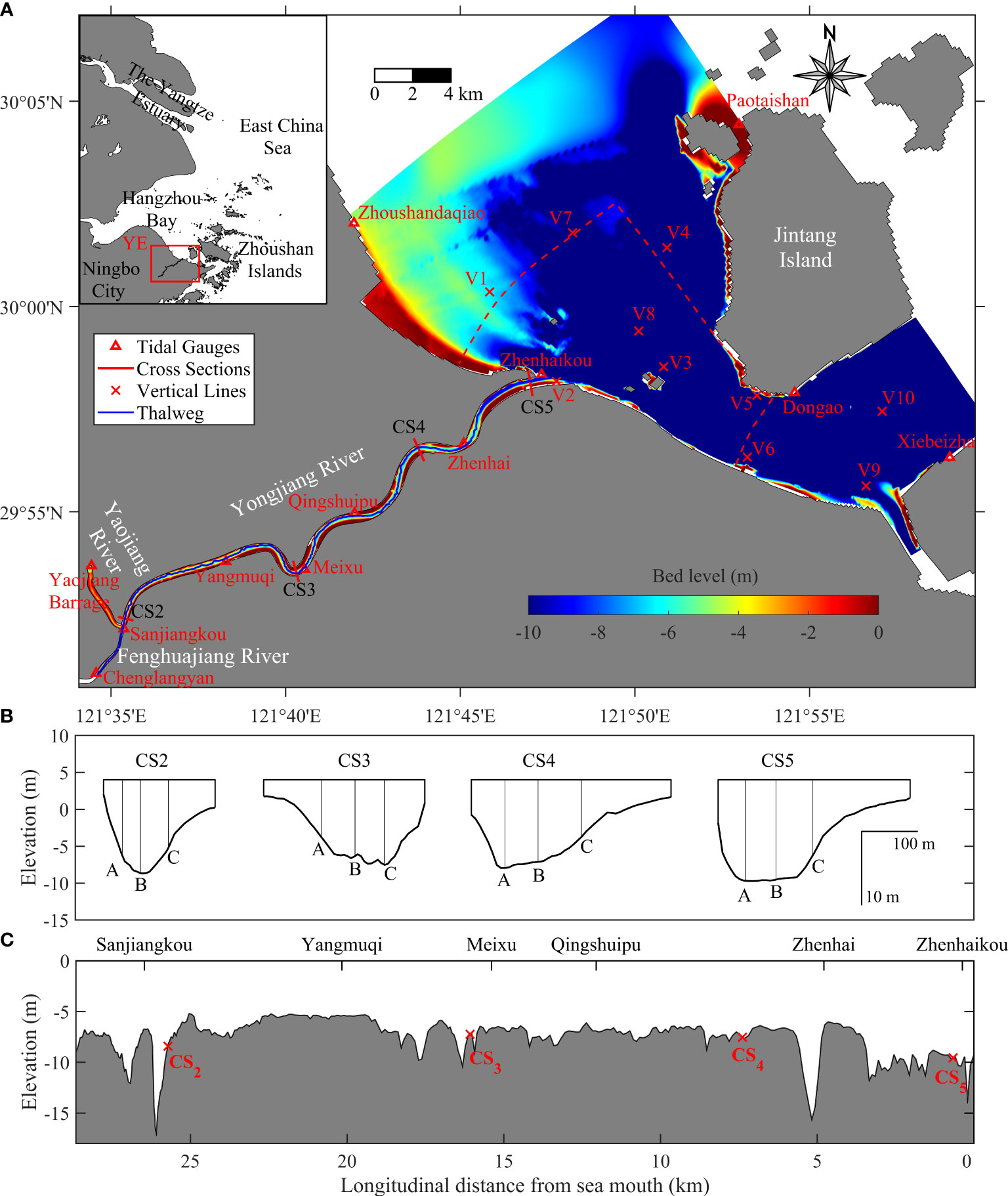
Figure 1 (A) Domain and bathymetry of the YE; (B) profiles of four measured cross sections (the view is looking seaward); (C) profile of the thalweg (the right origin denotes the river mouth). Areas covered by the color representing the bed level denotes the overall large model domain, and the red dashed line indicates the nested small model domain.
Our study focuses on the region between Zhenhaikou and Sanjiangkou in the YE, which is featured with tortuous geometry, narrow river channels (~300 m), and shallow water depth (~5 m). The YE is classified as a well-mixed estuary, and its sediment mainly comes from the adjacent sea area (Xiao et al., 2018). The tidal current in the adjacent sea area outside the YE is toward the northwest during flood tide and toward the southeast during ebb tide (Kuai et al., 2017). Water of high turbidity from the northern coast outside the YE (in the south of Hangzhou Bay) is transported to the vicinity of the river mouth by the ebb tide and then moves back toward the northwest or into the YE by the flood current. Historically, a number of hydraulic projects have been constructed in the Yongjiang River, including the Yaojiang barrage in 1959, the seawall in the river mouth in 1975, 17 large reservoirs, 18 bridges, 212 wharves, and many tidal and drainage gates situated on both sides of the river (Yan, 2011). Affected by the hydraulic structures, the equilibrium of the flow-sediment dynamics in the Yongjiang River has been broken, leading to remarkable siltation all over the river, and it has taken many years to achieve a new equilibrium. Since the construction of the Yaojiang barrage in 1959, the riverbed in the Yongjiang River has gone through the following six stages: intense deposition of the whole reach (1959–1961), gradual balance between the erosion and deposition (1962–1974), re-siltation while the balance was broken again (1975–1979), dynamic equilibrium of erosion and deposition (1980–1985), slow deposition (1986–2000), and deposition on the side shoal (2001–present) (Zhao et al., 2015).
3 Data and methodology
3.1 Sampling protocol
The field observations were conducted during spring and neap tides respectively in June 2015. During measuring, 12 sites at four cross sections (three sites at each cross section) were set in the YE, and 10 sites were set in the adjacent sea area (see detailed locations in Figure 1A). In each measured site, the horizontal tidal current velocity and direction, salinity, and SSC are synchronously measured at 0.0H, 0.2H, 0.4H, 0.6H, 0.8H, and 1.0H (H: the total water depth) each hour (refer to Xiao et al., 2018 for details).
Based on the simultaneous bathymetric surveying, lateral profiles of four cross sections CS2- CS5 and the longitudinal profile of the thalweg are displayed (Figures 1B, C). CS2 is located in the straight section, and its channel is relatively symmetric and slightly tilted to the left bank. CS3 is set at the sharp bend section of Meixu, with the deep channel tilted to the right bank. CS4 is situated near the bend of Zhenhai, and its channel is tilted to the left bank. CS5 lies at the bend just near the river mouth with its deep channel tilted to the left bank. An obvious channel–shoal system has been formed on the cross sections of the bends in the YE. Due to the lateral bathymetric variation, the longitudinal estuarine circulation will manifest a significant lateral structure (Alahmed et al., 2021) and will be accompanied by considerable lateral residual circulation.
3.2 Numerical model
A 3D numerical model of the YE is set up utilizing the Delft3D model system (Deltares, 2021), which simulates flow, salinity, and sediment transport. The horizontal and vertical directions of the model use orthogonal curvilinear and σ coordinates, respectively. Vertical mixing is computed with a k- ϵ turbulence model (Jones and Launder, 1972). The continuity and momentum equations of water motion respectively read:
and
where ξ, η and σ represent orthogonal curvilinear and σ coordinates; and are Lame coefficients; u, v, and ω are the current velocity components in the ξ, η and σ directions, respectively; d is the still water depth; ζ is the tidal level;ρ (ρ0) is the (reference) water density; the Coriolis force coefficient f=2Ωsinϕ (Ω is the angular velocity of the earth’s rotation, and ϕ is the local latitude); Fξand Fη are the horizontal Reynolds stress terms in the ξ and η directions, respectively; and υV is the vertical eddy viscosity coefficient.
The salinity and suspended sediment transport model satisfies the advection–diffusion equations as follows:
and
where s is the salinity; c is the SSC; ws is the settling velocity for sediment; and DH and DV are horizontal and vertical eddy diffusion coefficients, respectively.
In a previous study, the overall 2D depth-averaged hydrodynamic model of the YE was set up (refer to Kuai et al., 2017 for details), which captured well the 2D characteristics of water motion. Based on the previous larger model, a nested model with a smaller domain and higher grid resolution is established, in order to configure reliable boundary conditions for the salinity and SSC and save computing time and storage space. The overall model covered the entire YE and the adjacent sea region, which was north to Zhoushandaqiao, south to Xiebeizha, and upstream to Yaojiangzha and Chenglangyan. Its hydrodynamic boundary conditions were all given by observed temporal tidal-level variation from tide gauges deployed around model boundaries. The nested model (see the dashed line in Figure 1A) covers north to V1 and V7, south to V5 and V6, and its upstream extends to the same location as the overall one.
The hydrodynamic boundary conditions of the nested model are extracted from the overall one, and boundary conditions of salinity and SSC are extrapolated from each layer based on the observed data of the measured sites set near boundaries. The model has 403×174 cells with a high resolution in the river part (~100 m longitudinally and ~15 m laterally). The grid is gradually coarsening toward the outer sea (~150 m). Ten equidistant σ layers are prescribed over the vertical direction. The initial tidal level, current velocity, salinity, and SSC are all set to zero. At the closed boundaries, a no-transport condition due to impermeability is imposed, then normal components of the current velocity, salinity, and SSC gradient are set to zero. In order to calculate the accurate approximation of the horizontal gradients both in the baroclinic pressure term and in the horizontal diffusion term and reduce the truncation errors which may cause artificial vertical mixing and artificial flow (Stelling and Van Kester, 1994), the correction for σ coordinates (Deltares, 2021) is implemented to improve the accuracy of simulated salinity and stratification, especially at neap tide when the strong stratification occurs as described below. The erosion and deposition are calculated with the Partheniades-Krone formulation (Partheniades, 1965) for cohesive sediment. The 3D baroclinic model is calibrated with Manning’s n coefficient, which spatially varies from 0.018 to 0.025 s/m1/3 depending on the water depth. The calibrated parameters are summarized in Table 1.
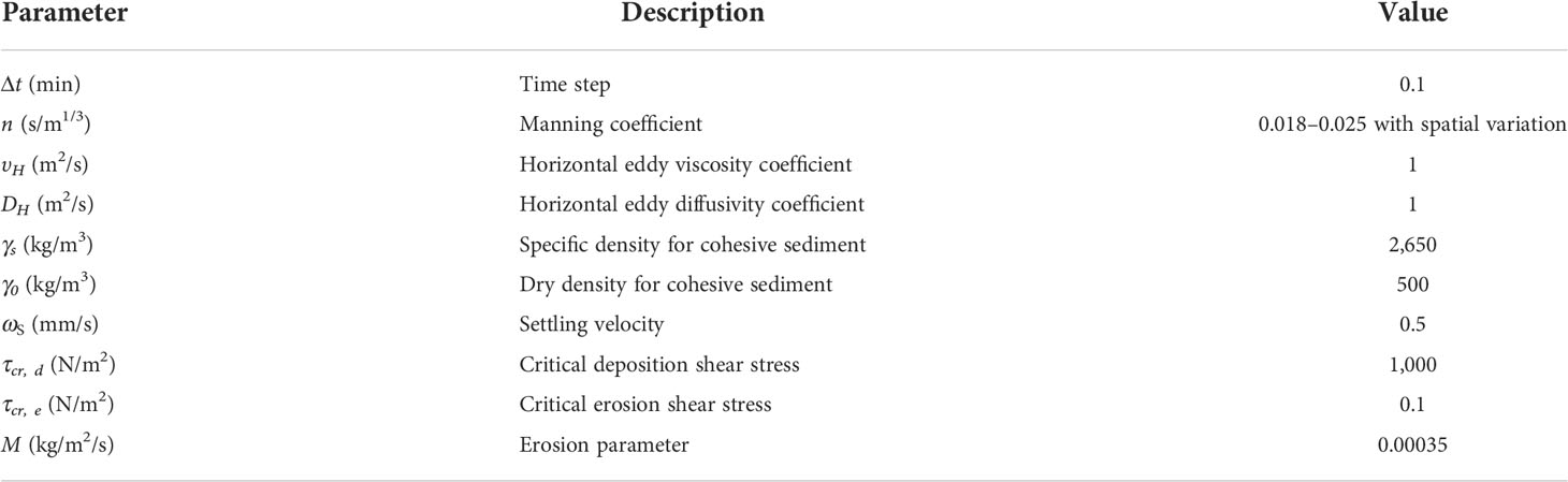
Table 1 Parameter settings in the model.
We have run a model simulation from 12 to 26 June 2015 (14 days), which has been validated extensively based on the data observed during spring and neap tides. The correlation coefficient (CC), skill score (SS), and root mean square error (RMSE) are calculated to assess the agreement between the simulation and the observation. The CC, SS, and RMSE are calculated as follows, respectively:
where xs and xo are model results and observations, respectively, and the overbar represents the mean value. The CC/SS represent the agreement between the model and the observations, with a CC/SS value of 1 indicating perfect agreement and a value of 0 indicating complete disagreement. The RMSE indicates the average deviation between the model results and the observations.
3.3 Data analysis methods
3.3.1 Residual current
The tidal dynamics are strong in the YE causing motion of saltwater and suspended sediment. The tide-induced residual current can better reveal the net transport trend of water, salinity, and suspended sediment. According to the mass transport flow theory (Robinson, 1983), the residual current of the layer k can be calculated as follows:
where the angle brackets denote a tidally averaged quantity, u is the longitudinal or lateral current velocity, subscript k refers to layer k, T is the tidal cycle, and Δzk is the water depth of layer k.
3.3.2 Momentum balance
According to Eq. (2), the longitudinal and lateral momentum balance is analyzed (Fugate et al., 2007), in order to find the mechanisms of the residual current. The left hand of the equation is the local acceleration term, and on the right hand, M1–M8 denote the longitudinal, lateral, and vertical advection, Coriolis force, barotropic and baroclinic pressure gradient, and horizontal and vertical momentum diffusion terms, respectively. Based on the calculated results, the vertical advection (M3) and horizontal and vertical momentum diffusion terms (M7 and M8) are small in magnitude and negligible; thus, only the longitudinal advection (M1), lateral advection (M2), Coriolis force (M4), barotropic pressure gradient (M5), and baroclinic pressure gradient (M6) terms are considered in the following analysis of their contribution to the residual current.
3.3.3 Residual sediment flux and decomposition
To explore the relative importance of various underlying physical processes in more detail, depth-integrated and tidally averaged suspended sediment flux (SSF) per unit width over both the longitudinal and lateral is calculated and decomposed into seven components (Uncles et al., 1985; Dyer, 1988; Burchard et al., 2018), as follows:
where the total water depth H= d+ ζ, the subscript t and d denote the deviations from the tidal and vertical means respectively, and the overbars signify the means over the depth.
F1 represents the mean flow induced transport, i.e., transport due to Eulerian flow; F2 is transport due to Stokes drift; and together F1 + F2 denotes the advective sediment flux (the Lagrangian flux) due to the residual flux of water and the tidally and vertically averaged SSC. F3, F4, and F5 are the tidal pumping terms (Uncles et al., 1985) that are generated by the phase differences between the depth-averaged SSC, the depth-averaged current velocity, and tidal level. F6 and F7 arise from the vertical circulation effects. Thus, the SSF is composed of three terms, which are advection, tidal pumping, and vertical circulation transport terms, respectively.
4 Results
4.1 Field data results
Based on Eq. (6), both the longitudinal and lateral residual currents at four cross sections are computed respectively during spring and neap tides (Figure 2). According to the measured results, the longitudinal residual current in the YE is -0.1 to 0.2 m/s generally, which decreases gradually from the surface to the bottom, and presents a significant lateral difference (Figures 2A, B). During the spring tide, the residual current at all cross sections shows an outflow trend and is stronger at CS5 near the river mouth, while the residual current of CS4 is weaker than that in the upper and lower reaches. During the neap tide, the deep channel of downstream CS4 and CS5 presents an exchange flow with inflow near the bottom and outflow at the surface, while the residual current at upstream CS2 and CS3 and shallow water regions (shoal) of downstream CS4 and CS5 are still controlled by runoff and each layer displays a stronger outflow trend.
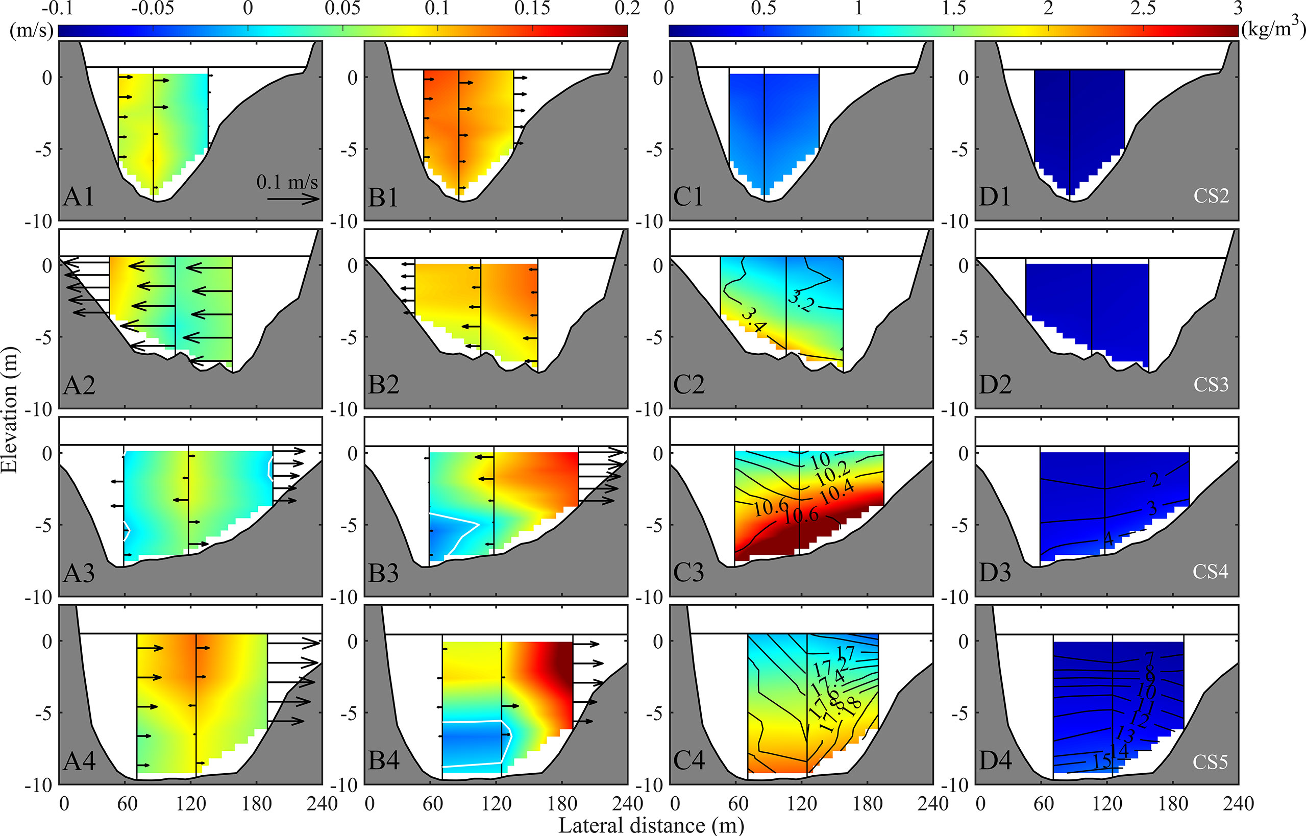
Figure 2 Observed lateral distribution of the longitudinal (color) and lateral (arrow) residual current at spring (A1–A4) and neap (B1–B4) tides, and the residual SSC (color, kg/m3) and salinity (contours, psu) at spring (C1–C4) and neap (D1–D4) tides. The white contours indicate the zero values of the longitudinal flow. The view is looking seaward. Positive values (red) for longitudinal flow indicate a seaward flow, while for lateral flows, positive is toward the right bank. Salinity is contoured in 0.2 and 1 psu at spring and neap tides, respectively. The absence of salinity contours indicates that the water within cross sections is freshwater. SSC, suspended sediment concentration.
The lateral water motion in the river channel generates a significant net transport, with its value ranging from -0.1 to 0.1 m/s, which is comparable to the magnitude of the longitudinal residual current. The lateral residual current presents quite different structures at various sites during spring and neap tides. At upstream CS2, the lateral flow is predominantly toward the shoal at both spring and neap tides, but its magnitude is small. At CS3 of the Meixu bend, the lateral residual current also tends to flow to the shoal, and the flow is stronger during spring tide (~0.1 m/s) than neap (~0.02 m/s). At CS4 of the Zhenhai bend, the deep channel shows a three-layer circulation structure with flow toward the convex bank in the upper and lower layers and toward the concave bank in the middle layer during spring tide, while a weak counterclockwise circulation emerges at neap tide, and the lateral flow on the shoal is toward the convex bank both at spring and neap tides with its value up to 0.05 m/s. At CS5 of the Zhenhaikou river mouth, the lateral flow is generally toward the shoal of the convex bank during spring tide and shows a clockwise circulation regionally, while during neap tide the deep channel presents a weak counterclockwise circulation with a strong shoreward current on the shoal (~0.05 m/s).
The SSC at upstream CS2 is relatively low and generally not affected by salinity. At CS3 of the Meixu bend, the isohalines generally slope downward toward the right bank and the suspended sediment is accumulated on the shoal of the left bank at spring tide (Figure 2C2), which is consistent with residual flow toward the convex bank near the bottom (Figure 2A2). Due to the tidal current weakening at neap tide, the salinity and SSC at CS3 become very low. At downstream CS4, the lateral flow toward the convex bank in the lower layer (Figures 2A3, B3) causes suspended sediment trapped on the shoal of the right bank, and the isohalines are slightly lifted toward the surface of the shoal of the right bank which means that high salinity accumulates near the bottom of the right bank (Figures 2C3, D3). At CS5 of the river mouth, the contours of SSC are horizontally distributed and the SSC at the deep channel is slightly higher than that at the shoal, i.e., no obvious lateral sediment trapping occurs.
During spring tide, there is no significant lateral variation of residual salinity in each cross section, and the stratification is quite weak with the maximum difference between the surface and bottom salinity only 1.5 psu. However, at neap tide, a conspicuous stratification emerges near the river mouth area, with the maximum difference between the surface and bottom salinity up to 3 and 10 psu at CS4 and CS5, respectively. Due to the weaker tidal current during the neap tide, the saltwater intrusion distance is much shorter than that of spring tide, which causes a larger longitudinal salinity gradient. Both the vertical stratification and longitudinal salinity gradient at neap tide are stronger as compared with the spring tide, so the larger baroclinic effect will drive the longitudinal residual circulation near the river mouth.
In the longitudinal direction of the river channel, the SSC at CS4 during spring tide is significantly higher than that of upper and lower reaches (Figure 2C3), exhibiting an obvious ETM phenomenon, which is consistent with the weaker longitudinal flow here (Figure 2A3). While during neap tide, the SSC in the YE is greatly reduced because of the weaker tidal current with the spatial distribution decreasing gradually from the river mouth to the upper reaches; thus, no obvious ETM exists inside the river mouth.
The suspended sediment is laterally trapped on the shoal of the convex bank at both CS3 and CS4, which can easily cause deposition in the shoal. It is noteworthy that regardless of spring and neap tides, the lateral residual current near the bottom of each cross section at the bend demonstrates a net transport to the shoal of the convex bank. The salinity and SSC increase gradually from the surface to the bottom; thus, the lateral motion of bottom water determines the net depth-integrated transport of salt and suspended sediment, which will play an important role in the lateral sediment trapping. This pattern of lateral flow agrees with the suspended sediment laterally trapped on the shoal described.
4.2 Numerical results
4.2.1 Model validation
The validation of the tidal level, current velocity, current direction, salinity, and SSC on 17 to 26 June 2015 at some measured stations is shown in Figure 3. During spring–neap tidal cycles, the overall CC/SS/RMSE of the tidal level, current velocity, direction, salinity, and SSC are 0.99/0.97/0.10, 0.86/0.88/0.15, 0.91/0.85/11.30, 0.81/0.80/2.02, and 0.57/0.61/0.59, respectively. They are averaged from four cross sections in the lower, middle, and upper layers. Although the CC and SS of SSC are slightly lower than those of hydrodynamic variables due to the extremely complicated suspended sediment processes, the twin peak SSC signals inside the river mouth during a semidiurnal tidal cycle is well reproduced by the model (Figure 3E). Therefore, the model is proved to be able to reliably reproduce the flow movement and salinity and suspended sediment transport processes in the YE.
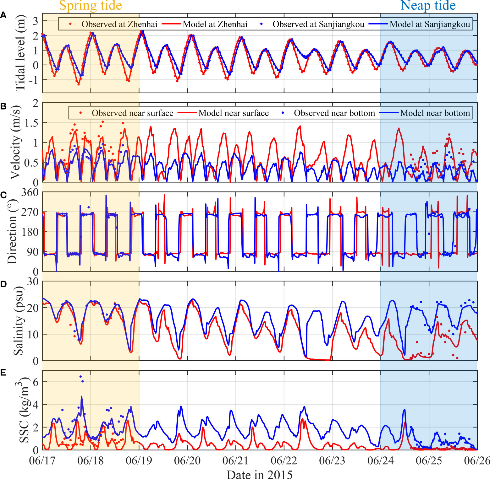
Figure 3 Model-data comparison between observed (dot) and simulated (line) results for tidal level (A) at Zhenhai (red) and Sanjiangkou (blue), current velocity (B), current direction (C), salinity (D), and SSC (E) near surface (red) and bottom (blue) at the measured site CS5B, respectively. SSC, suspended sediment concentration.
4.2.2 Lateral distribution of residual flow and SSC
In order to reveal mechanisms of the residual flow and sediment trapping along the YE, eight transects S1–S8 are selected from Zhenhaikou to Meixu (Figure 4A). Transects S1, S4 and S8 separately correspond to CS5, CS4, and CS3. Transects S2, S5 and S7 suited the bends between Meixu and Zhenhai. Transects S3 and S6 are located in the transition straight reaches near Qingshuipu and Zhenhai, respectively. Both S3 and S6 transects are relatively wide, shallow, and symmetrical, and there is no obvious structure like transects at bends where the deep channel is located near the concave bank and the shoal is located near the convex bank.
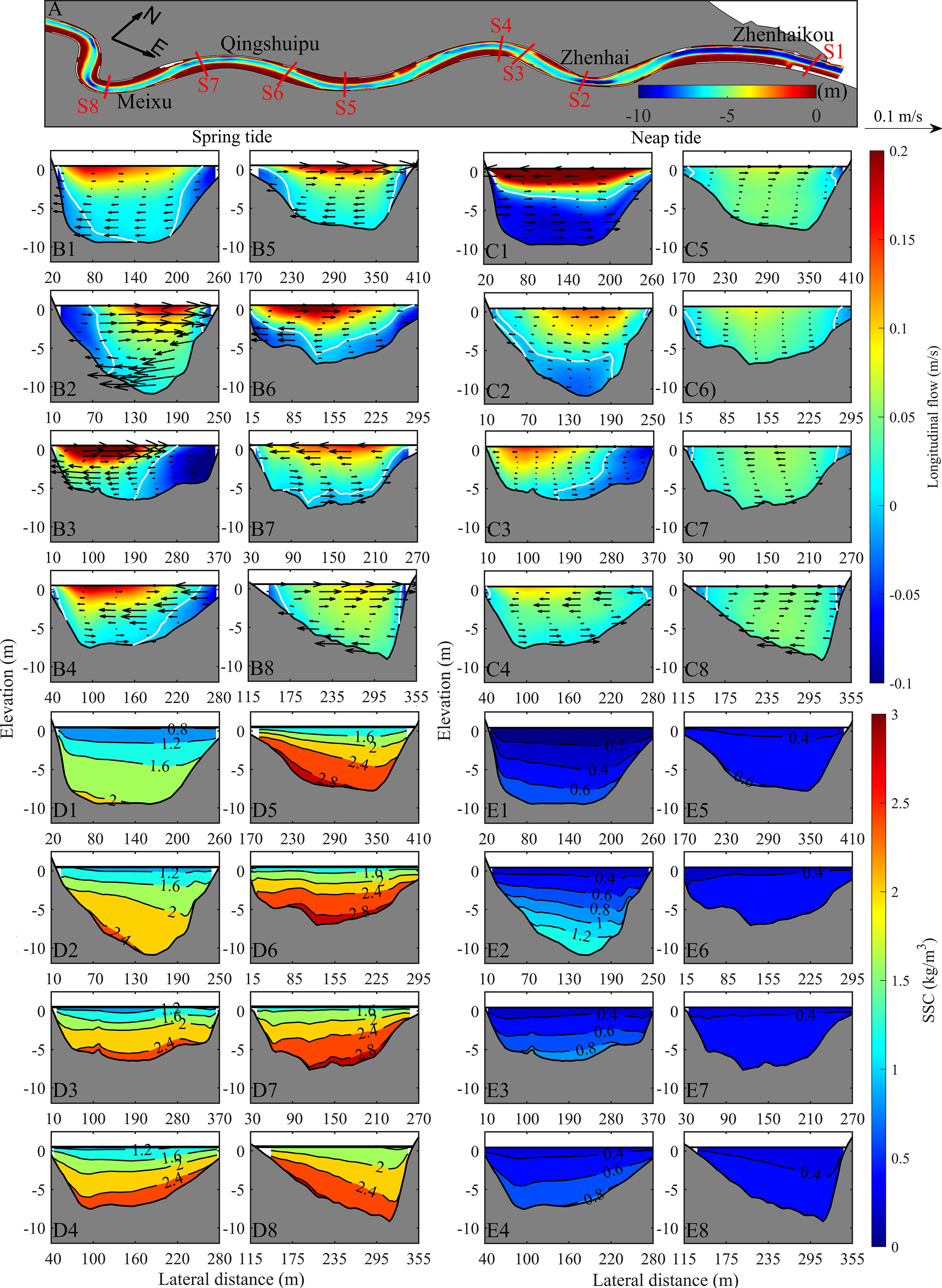
Figure 4 Patterns of residual flow and SSC at eight selected transects S1–S8 (A, color indicates the bed level). Lateral distribution of the longitudinal (color) and lateral (arrow) residual current at spring (B1–B8) and neap (C1–C8) tides, and the residual SSC during spring (D1–D8) and neap (E1–E8) tides is displayed. SSC is contoured in 0.4 and 0.2 kg/m3 at spring and neap tides, respectively. The view is looking seaward. SSC, suspended sediment concentration.
The residual current of each transect is calculated according to the simulated results (Figures 4B, C). During spring tide, the residual flow at these transects shows an outflow trend except S6 and S7. There is a weak landward residual flow at the bottom of transects S6 and S7 (Figures 4B6, B7). During neap tide, the residual flow at upstream transects still demonstrates an outflow trend, while near the river mouth, the flow in the lower layer is landward (Figures 4C1–C3), and that in the upper layer is seaward, generating the estuarine circulation here.
In the curved reaches, transects S2, S5, S7, and S8 show a circulation structure with flow toward the concave bank at the surface and toward the convex bank near the bottom during spring tide (Figures 4B2, B5, B7, B8). The surface residual flow at transect S1 is toward the convex bank, while the bottom flow is toward the concave bank, forming a clockwise circulation (Figure 4B1). The lateral flow at transect S4 presents a three-layer circulation structure as described above (Figures 2A3, 4B4). During neap tide, the lateral residual current at transects S2, S4. S5, S7, and S8 is toward the concave bank at the surface and toward the convex bank near the bottom. The circulation pattern at transect S1 is opposite to that of the spring tide, with flow toward the concave bank at the surface and toward the convex bank near the bottom.
In the transition straight reaches, the lateral circulation structure is different from that of the curved reaches. During spring tide, it presents a double-cell lateral circulation structure with surface convergence and bottom divergence at both sides of the transects S3 and S6 (Figures 4B3, B6). The lateral residual flow is weak during neap tide but still presents a divergent trend near the bottom (Figures 4C3, C6).
The distribution of the tidally averaged SSC of eight transects is shown in Figures 4D, E. Along the river channel, the tidally averaged SSC at spring tide reaches the maximum between transects S5 and S7 with its value up to 2.8 kg/m3, indicating that the suspended sediment is longitudinally trapped in the Qingshuipu reach (Figures 4D5–D7). During neap tide, the maximum SSC zone shifts downstream to the vicinity of transect S2, with its value reduced to 1.2 kg/m3 due to the weakening of the tidal current, i.e., the sediment is longitudinally captured in the Zhenhai reach.
Along the cross section of the river, the high turbidity does not always aggregate in the deep channel, but it will be laterally trapped on the shoal to some extent. The contours of the SSC at the Zhenhai bend (transects S2 and S4), Qingshuipu bend (transects S5 and S7), and Meixu bend (transect S8) are all lifted toward the surface of the shoal of the convex bank, especially transect S8 (Figure 4D8). Its high-turbidity zone spreads to the surface along the shoal of the convex bank, and obvious lateral sediment entrapment emerges here. While at the river mouth bend (transect S1) and transition straight reaches (transects S3 and S6), no obvious deflection of the high-turbidity zone occurs, indicating that the lateral sediment trapping is weak, and the sediment mainly aggregates in the deep channel.
4.2.3 Longitudinal distribution of residual flow and SSC
Figure 5 shows the pattern of longitudinal residual current along the thalweg of the YE. During spring tide, the flow shows an outflow trend for each layer but a weak inflow at the bottom of some regions exists. During neap tide, the residual flow in the upper reaches is still seaward, but a really stng estuarine circulation emerges within about 7 km upstream from the river mouth, which is seaward at the surface and landward near the bottom. This is consistent with the previous analysis of the observations (Figures 2A, B).
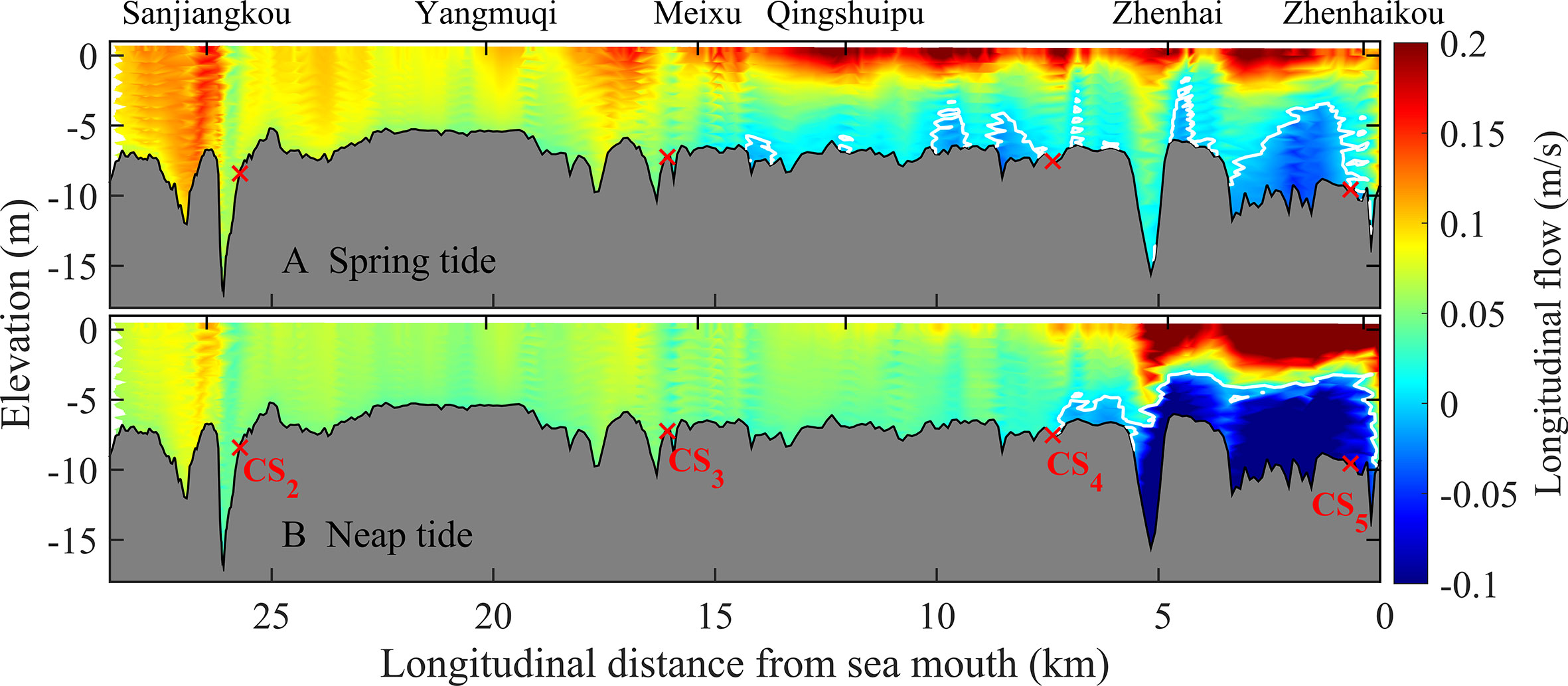
Figure 5 Distribution of the longitudinal residual current in the thalweg at spring (A) and neap (B) tides. The white contours indicate the zero values of the longitudinal flow. Positive values (red) for longitudinal flow indicate a seaward flow. The right origin denotes the river mouth.
During spring tide, the isohalines are generally vertical, i.e., the vertical mixing of salinity is relatively strong. The salt intrusion can be as far as the vicinity of Yangmuqi (Figure 6A). During neap tide, salinity near the river mouth is significantly stratified with the maximum difference between the surface and bottom salinity up to 10 psu. The salt intrusion becomes weaker and can only be up to Qingshuipu. The distance of salt intrusion is about 7 km shorter than that of spring tide, resulting in a larger longitudinal density gradient (Figure 6B).
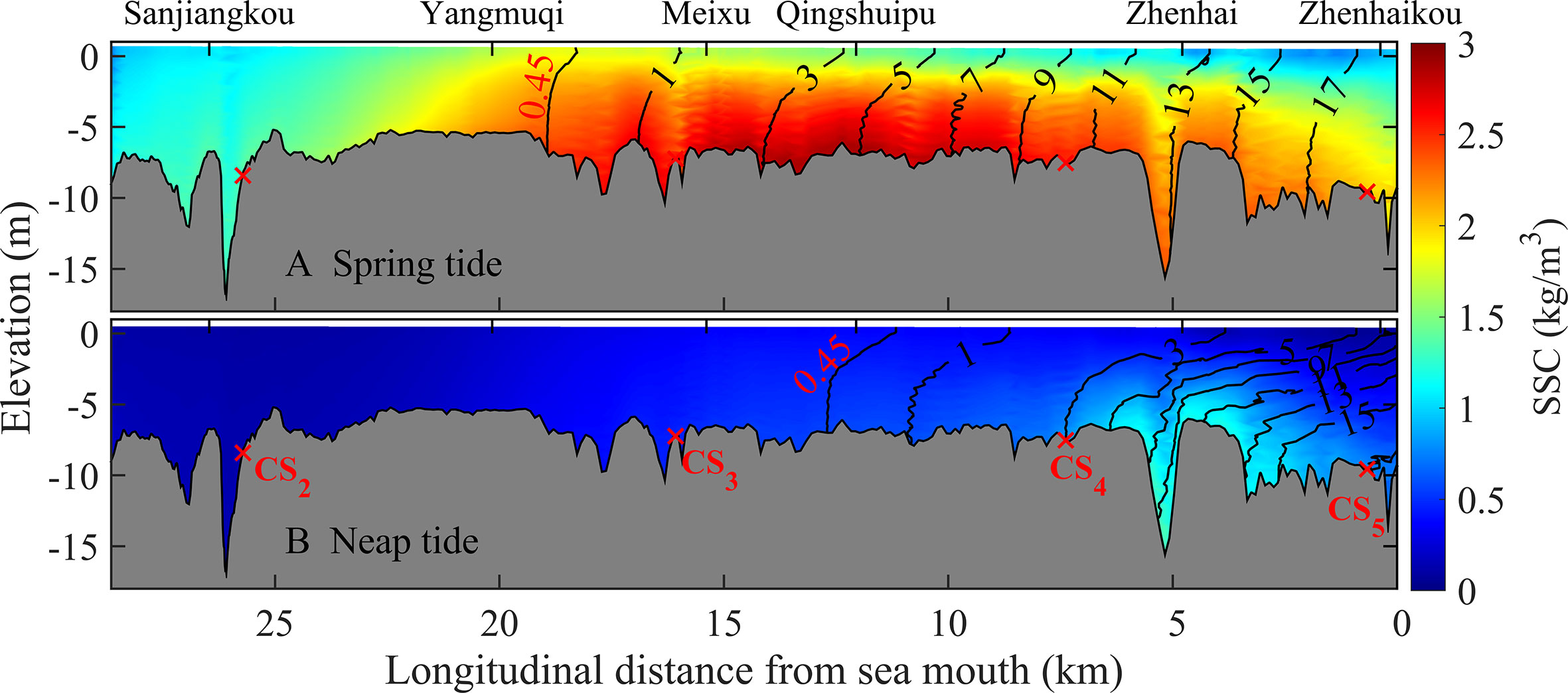
Figure 6 Distribution of the residual SSC (color, kg/m3) and salinity (contours, psu) in the thalweg at spring (A) and neap (B) tides. Salinity is contoured in 2 psu, and the salinity 0.45 psu represents the limit of the saltwater intrusion. The right origin denotes the river mouth. SSC, suspended sediment concentration.
The SSC reaches its maximum of about 12 km upstream from the river mouth during the spring tide (Figure 6A), so the ETM of the YE is situated near Qingshuipu. However, the ETM moves downstream to Zhenhai (~5 km from the river mouth) at neap tide. It indicates that the ETM will gradually shift downstream with the tidal current weakening. Corresponding to Figure 5, the ETM core area during spring tide is located around the front of the bottom inflow near Qingshuipu, and during neap tide located on the front of the strong exchange flow inside the river mouth.
The intratidal motion of the ETM at typical times during spring tide is displayed in Figure 7. At early flood, the ETM is mainly accumulated within about 4 km upstream from the river mouth (Figure 7A), as a result of the high turbidity seawater flowing into the YE from the adjacent sea area (Xiao et al., 2018) with the flood tide. As the flood current strengthens, the high SSC zone further moves toward the upper reaches up to the vicinity of Yangmuqi (Figure 7B). At later flood, the sediment begins to settle and the ETM continues to go upstream as far as Sanjiangkou with the flood current weakening (Figure 7C). During early ebb, a large amount of sediments is deposited and the ETM narrows and moves downstream to the vicinity of Meixu (Figure 7D). As the ebb current strengthens, the SSC of the ETM gradually increases and continues to be transported downstream to the river mouth and then decreases as the current weakens (Figure 7E). Then, the ETM will move to and fro with the next tidal cycle, which carries the high-turbidity water into the estuary again. It can be found that during spring tide, sediment is trapped in the vicinity of Qingshuipu (Figure 6A) and the ETM moves on a large scale within the Yongjiang River (Figure 7). They are important reasons for severe siltation in the whole reach (Yan, 2011).
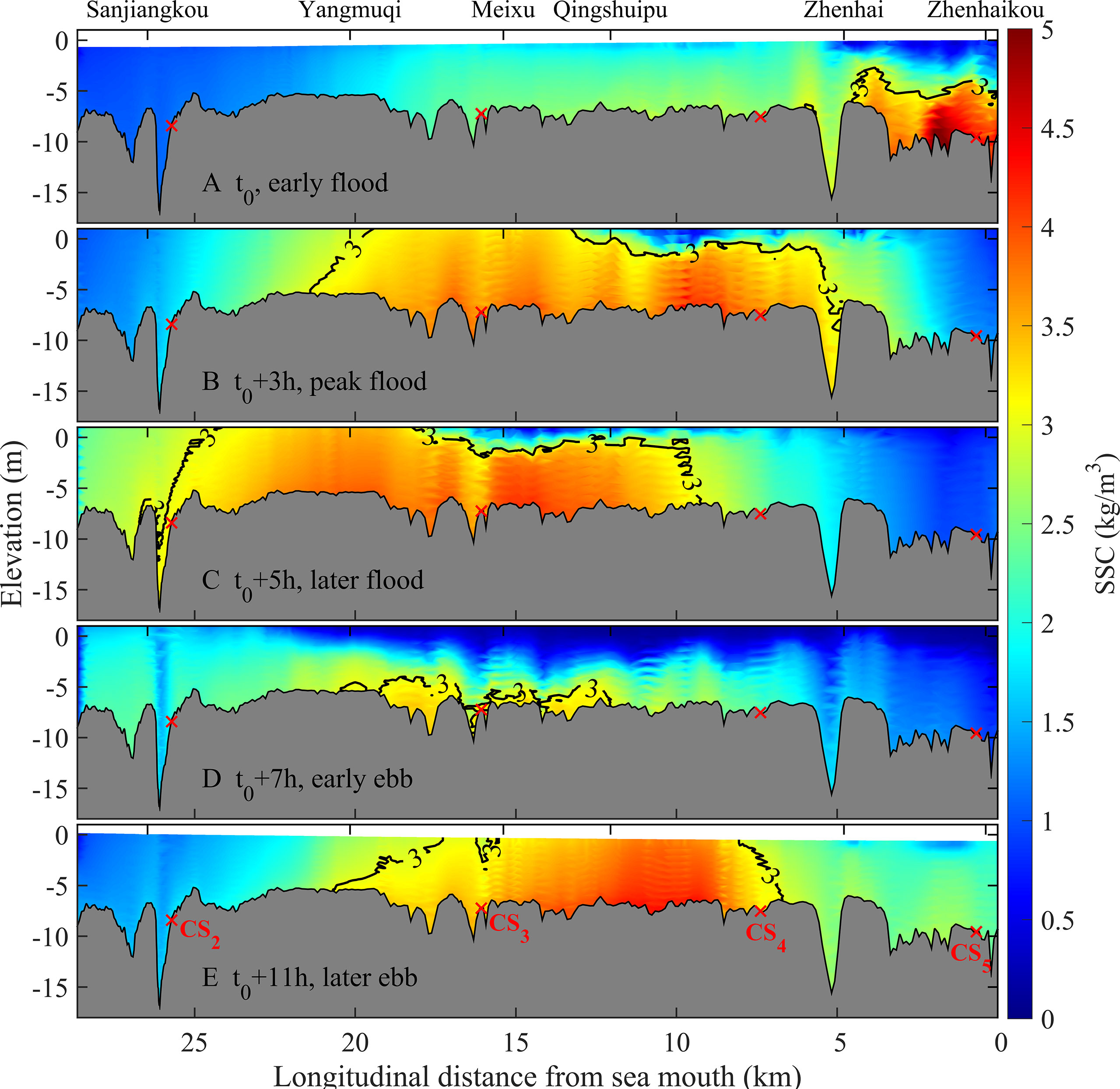
Figure 7 Intratidal motion of the ETM at typical time during spring tide including early flood (A), peak flood (B), later flood (C), early ebb (D) and later ebb (E). The black line indicates that the SSC is 3 kg/m3, and areas encircled by the blackline and riverbed indicate the high-turbidity zone. The right origin denotes the river mouth. ETM, estuarine turbidity maximum.
4.2.4 Residual sediment transport and morphological changes
By Eq. (7), the residual SSF are shown in Figure 8. Due to the stronger current and higher turbidity, the SSF at spring tide (~1.5 kg/(m·s)) is generally larger than that of the neap tide (~0.5 kg/(m·s)). At spring tide, sediment between Zhenhaikou and Qingshuipu is mainly transported landward, while sediment between Meixu and Qingshuipu is flushed downstream (Figure 8A), which causes the transport convergence at Qingshuipu. Thus, much sediment is trapped here, forming the ETM around Qingshuipu (Figure 6A). Sediment at the river mouth is exported, which may be caused by the tidal current in the outer-estuary regions. At neap tide, the convergence of sediment transport also exists but shifts downstream to the vicinity of Zhenhai (Figure 8B), similarly forming the ETM around Zhenhai (Figure 6B). Because of the strong exchange flow inside the river mouth at neap tide, the landward transport in the lower reaches of Zhenhai is stronger than the seaward transport in the upper reaches.
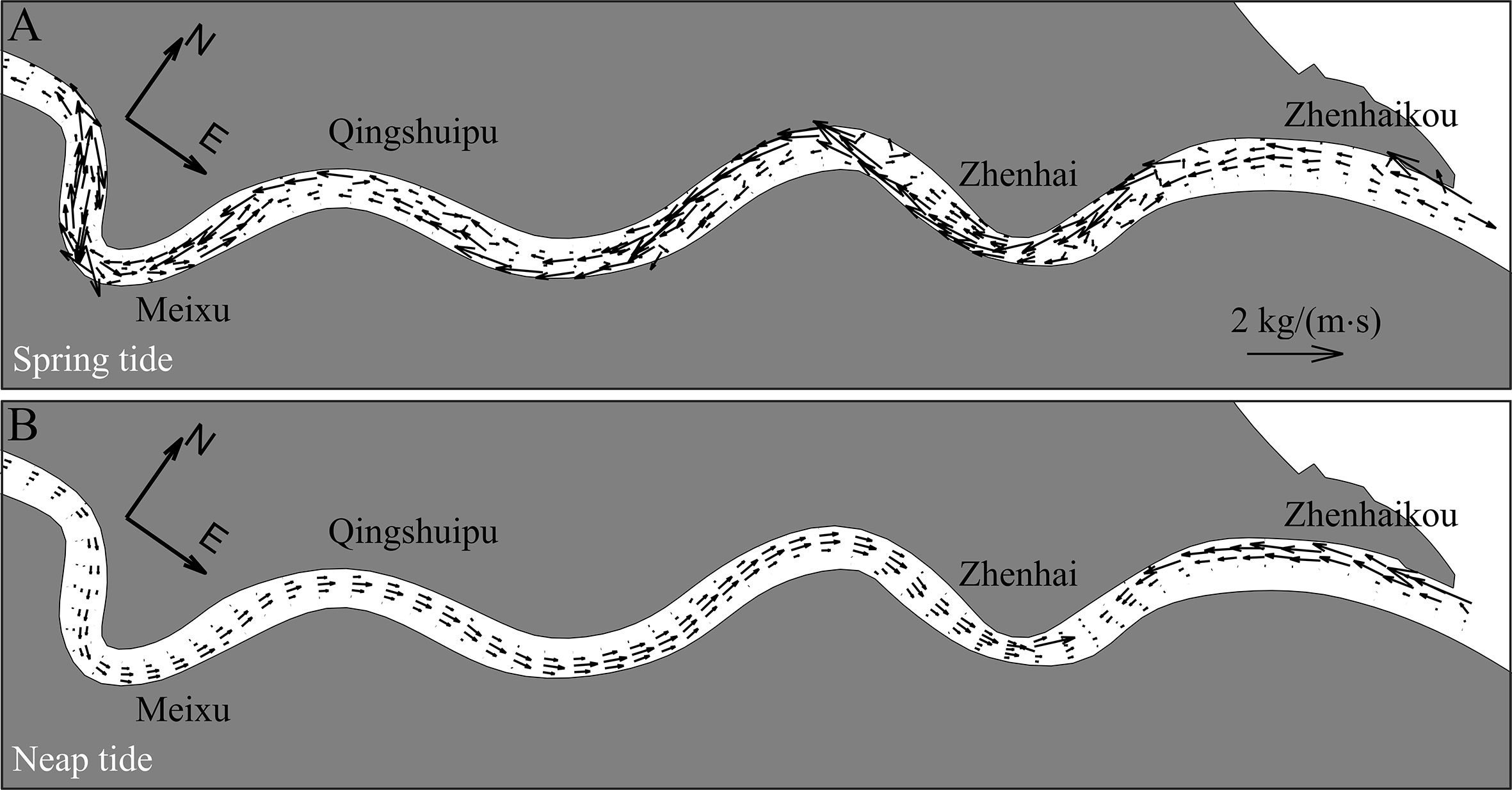
Figure 8 Distribution of residual SSF in the YE at spring (A) and neap (B) tides. The north direction is rotated by 35° clockwise. SSF, suspended sediment flux; YE, Yongjiang estuary.
The model has also simulated the riverbed evolution in the YE (Figure 9). Compared with the water depth, the bathymetry change (up to ~0.3 m) is relatively small within the whole simulation period (14 days). Therefore, the feedback of bathymetry change on the flow and sediment dynamics is not considered (Zhu et al., 2021). After 7 days, i.e., at spring tide, erosion generally occurs in the deep channel while deposition occurs in the shoal with both the value up to 0.3 m (Figure 9A), which is consistent with the suspended sediment laterally trapped on the shoal described above. In the Zhenhai reach, deposition occurs both in the shoal and in the channel. One of the primary reasons is that the larger depth here provides the area for sediment and salinity to accumulate and create a stratified region to promote the retention of sediment in the deep channel (Yellen et al., 2017). Severe deposition occurs just outside the pink contours near the junction area of the channel–shoal. However, the deposition is weaker in the shoal near the bank because of the weak current and low turbidity. After 14 days, i.e., at neap tide (Figure 9B), the erosion and deposition pattern of the riverbed is similar to that of spring tide. Nevertheless, the erosion in the Qingshuipu reach becomes stronger and the deposition becomes stronger between Zhenhai and Zhenhaikou. At the Zhenhaikou bend, contrary to erosion in the deep channel at spring tide, a deposition pattern is presented, which is caused by the weakening of the tidal current and sediment trapped around Zhenhai during neap tide.
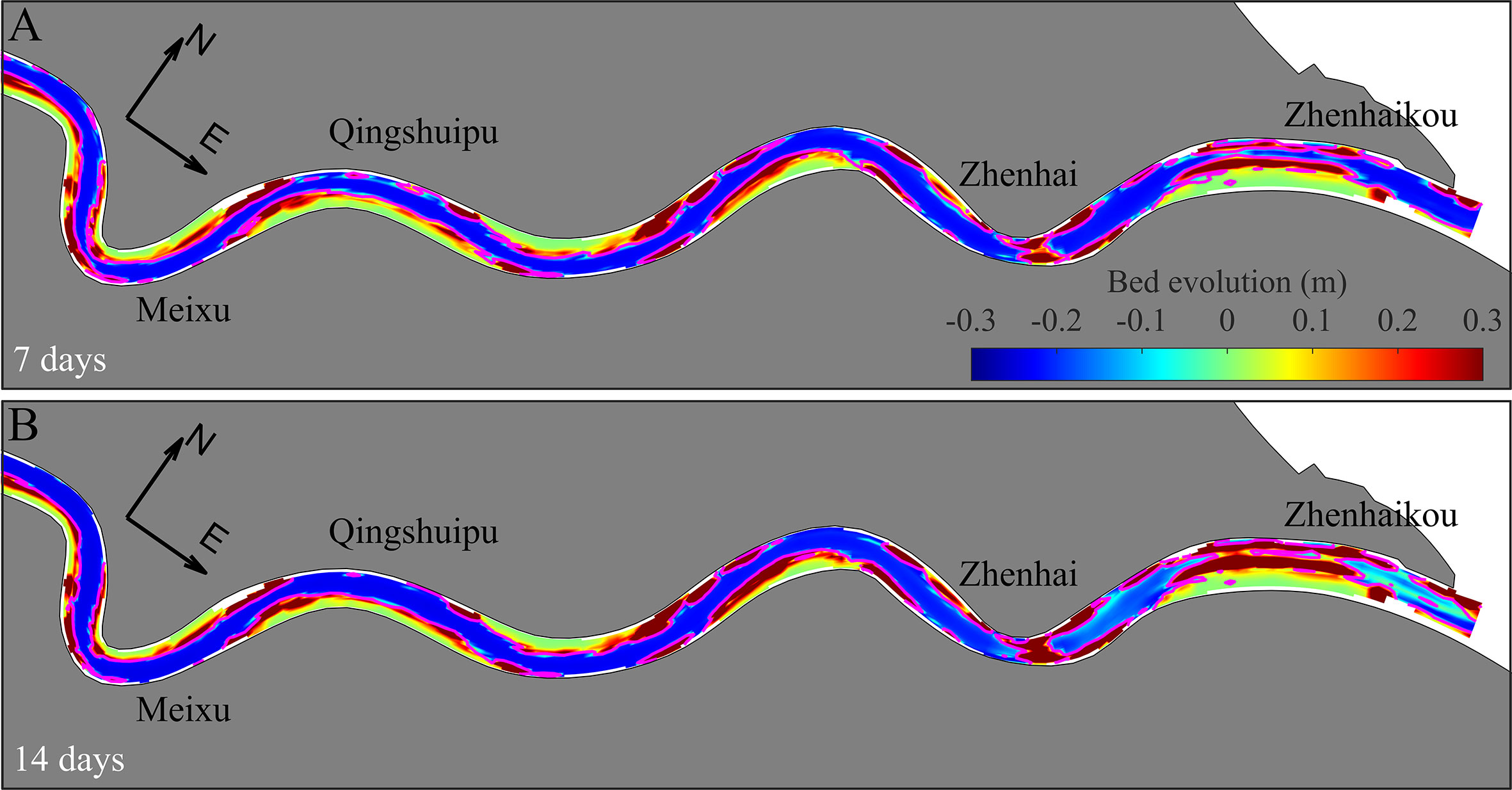
Figure 9 Pattern of bed evolution in the YE after 7 (A) and 14 (B) days. The north direction is rotated by 35° clockwise. Positive values (red) indicate deposition. The pink contours indicate the zero values of the bed evolution. YE, Yongjiang estuary.
5 Discussion
5.1 Momentum balance mechanisms
Based on the momentum balance analysis, the tidally averaged results of each momentum term at the right hand of Eq. (2) are calculated in the vertical direction of each transect center (Figures 10A, B). The contribution of each mechanism to the residual current is analyzed.
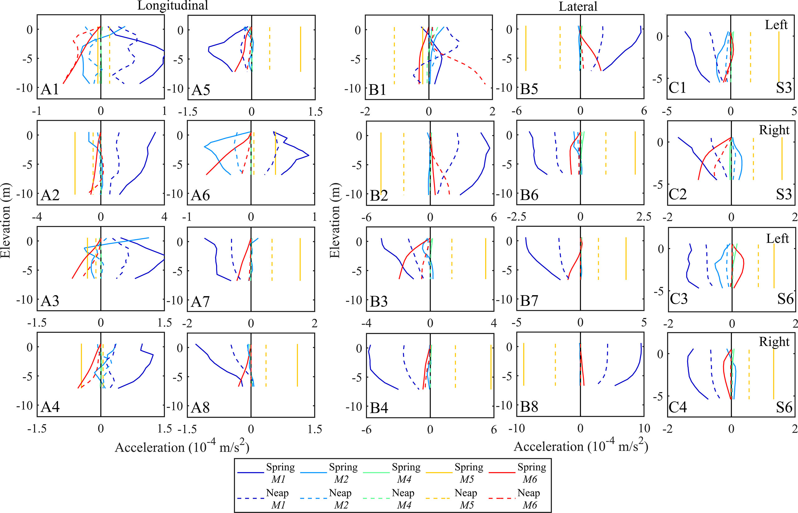
Figure 10 Momentum balance analysis of eight selected transects. The longitudinal (A1–A8) and lateral (B1–B8) momentum balance analysis in the vertical line of each transect center, and lateral momentum balance analysis of transects S3 (C1, C2) and S6 (C3, C4) calculated in the 1/4 (left) and 3/4 (right) of the river width away from the left bank are displayed. M1, M2, M4, M5 and M6 indicate the longitudinal advection, lateral advection, Coriolis force, barotropic pressure gradient, and baroclinic pressure gradient terms in Eq. (2). Positive is toward the river mouth and right bank for the longitudinal and lateral directions, respectively.
The longitudinal residual flow at Qingshuipu and its upper reaches are dominated by the barotropic pressure gradient during the spring tide (Figures 10A5–A8), while the residual flow at Zhenhai and its lower reaches are dominated by the longitudinal advection (Figures 10A1–A4). Although a large landward baroclinic pressure gradient exists near the bottom at the downstream transects of Zhenhai, it cannot counteract the seaward flow generated by the longitudinal advection. The weak landward residual flow at the bottom of transects S6 and S7 (Figures 4B6, B7) is caused together by the larger baroclinic pressure gradient, longitudinal advection, and lateral advection (Figures 10A6, A7). During neap tide, the residual flow at upstream transects is still dominated by the barotropic pressure gradient like during spring tide, while near the river mouth, the inflow in the lower layer is generated by a considerable baroclinic pressure gradient (Figures 4C1–C3), and the outflow in the upper layer is dominated by the longitudinal advection.
During spring tide, the salinity between transects S7 and S8 is relatively small. Therefore, the lateral baroclinic pressure gradient is weaker than the other forces (Figures 10B7, B8). The barotropic pressure gradient and longitudinal advection are dominant factors in the lateral momentum balance. At transects S5 and S6, the influence of salinity on the lateral residual current becomes more significant, accompanied by a relatively large baroclinic pressure gradient (Figures 10B5, B6). Although the barotropic pressure gradient and longitudinal advection effects still dominate, the existence of the baroclinic pressure gradient changes the momentum balance dominated only by the barotropic pressure gradient and longitudinal advection. It can generate the residual circulation toward the concave bank at the surface and toward the convex bank near the bottom. At transect S1, the surface residual flow is dominated by the lateral advection and Coriolis force, while the bottom flow is caused by the baroclinic and barotropic pressure gradient (Figures 4B1, 10B1). At transect S2, the lateral baroclinic pressure gradient is weak (Figure 10B2), so the lateral momentum balance is the same as that without the effect of salinity. The lateral flow at transect S4 in the upper and lower layers is dominated by the barotropic pressure gradient term, while the flow in the middle layer is dominated by the longitudinal advection, baroclinic pressure gradient, and lateral advection (Figure 10B4). Although the baroclinic pressure gradient is large at transect S5, its magnitude is not enough to shift the direction of the circulation structure, so the lateral momentum balance is the same as transects S2, S7, and S8.
Compared with the spring tide, the intensity of salt intrusion weakens during the neap tide. Thus, the lateral momentum balance at transect S5 is no longer controlled by the baroclinic pressure gradient. The lateral residual current at Qingshuipu and its upper reaches are dominated by the longitudinal advection at the surface and by the barotropic pressure gradient near the bottom. The opposite circulation pattern at transect S1 is caused by the opposite baroclinic pressure gradient. It is dominated by the barotropic pressure gradient at the surface and the baroclinic pressure gradient near the bottom. This momentum balance is completely different from that of spring tide. Despite the large baroclinic pressure gradient at transects S2 and S4, its magnitude is insufficient to transform the overall structure of the circulation.
In summary, the baroclinic pressure gradient can significantly affect the pattern of the estuarine circulation. It not only drives the landward residual current at the bottom of some reaches near Qingshuipu during spring tide and the vertical exchange flow near the river mouth but also shifts the lateral flow structure in the reaches closer to the river mouth. Therefore, the baroclinic pressure gradient plays an important role in the formation of the lateral residual circulation in the lower reaches that is greatly affected by salt intrusion.
In addition, in order to illustrate mechanisms of the double-cell circulation in the transition straight reaches respectively near Qingshuipu and Zhenhai, the vertical distribution of each momentum term at the right hand of Eq. (2) is calculated in the 1/4 and 3/4 of the river width away from the left bank, respectively (Figure 10C). On the left side of the channel, the divergent flow at the bottom, dominated by the longitudinal and lateral advection, is toward the left bank. On the right side, the divergent flow directs toward the right bank due to the barotropic pressure gradient dominated. Besides, the convergent flow at the surface is toward the right bank at the left side caused by the barotropic pressure gradient and toward the left bank at the right side caused by the longitudinal advection.
5.2 Residual sediment flux decomposing
According to Eq. (7), Figures 11 and 12 present the residual sediment flux and its decomposition along the longitudinal channel and lateral eight transects. The total sediment transport is composed of advection (F1+F2), tidal pumping (F3+F4+F5), and circulation transport (F6+F7). At spring tide (Figure 11A), sediment is mainly imported in the lower reaches 12 km away from the river mouth, which is dominated by the landward tidal pumping transport (up to ~2 kg/(m·s)). In the upper reaches, due to the seaward advection-dominated transport (~1 kg/(m·s)), sediment is mainly exported. The landward circulation transport in the YE is generally small (<0.4 kg/(m·s)). Thus, upstream seaward advection transport and downstream landward tidal pumping transport generate the transport convergence in the reach 12 km away from the river mouth, i.e., the vicinity of Qingshuipu (Figure 6A), forming the ETM around Qingshuipu during spring tide. At neap tide (Figure 11B), the sediment transport becomes weaker than that of spring tide. The effect of circulation transport becomes significant near the river mouth. In the lower reaches (~5 km away from the river mouth), sediment is mainly imported by the landward circulation (up to ~0.3 kg/(m·s)) and tidal pumping transport (up to ~0.5 kg/(m·s)). In the upper reaches, sediment is exported by the seaward advection (~0.2 kg/(m·s)) and tidal pumping transport (~0.2 kg/(m·s)). Because the strong exchange flow exists, circulation transport becomes significant near the river mouth. However, in the upper reaches 7 km away from the river mouth, it almost disappears. Thus, upstream seaward advection and tidal pumping transport and downstream landward circulation and tidal pumping transport generate the transport convergence in the reach 5 km away from the river mouth, i.e., the vicinity of Zhenhai (Figure 6B), forming the ETM around Zhenhai during neap tide.
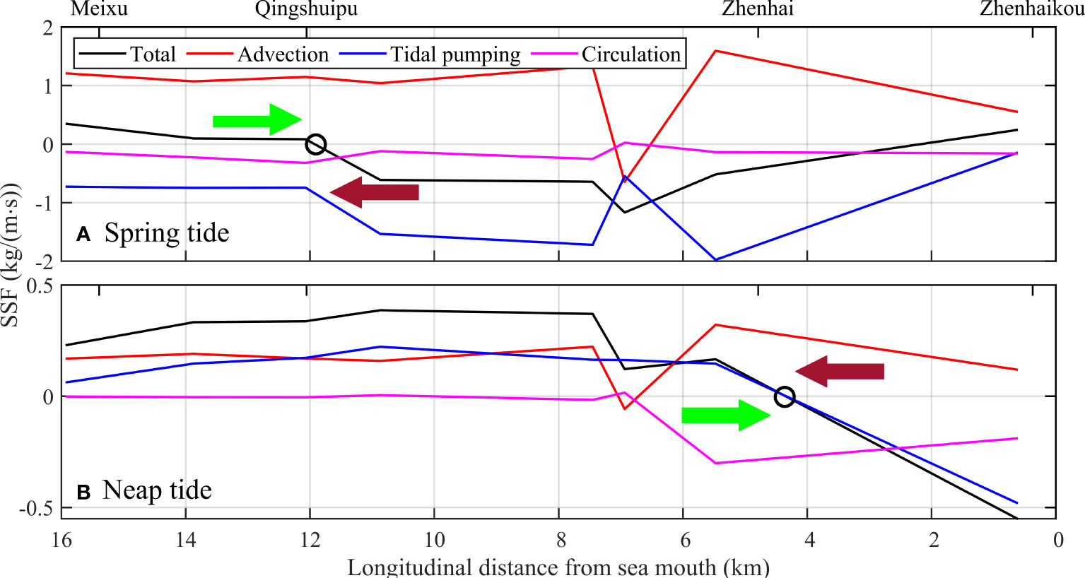
Figure 11 Distribution of longitudinal residual SSF and decomposition at eight transects during spring (A) and neap (B) tides. Longitudinal SSF is calculated in the vertical line of each transect center, and the right origin denotes the river mouth. Positive values indicate seaward flux. Colored arrows indicate the direction of total sediment transport. Hollow black circles indicate convergence of the sediment transport, i.e., sediment trapping. SSF, suspended sediment flux.
Although the lateral residual SSF is much smaller (~0.1 kg/(m·s)) than longitudinal ones (Figure 12), the lateral transport is extraordinarily important for the lateral sediment entrapment. At transect S1, sediment transport is dominated by the advection transport toward the left bank at spring tide (Figure 12A1) and by the tidal pumping and circulation transport toward the right bank at neap tide (Figure 12B1), respectively. It is consistent with the opposite circulation structure (Figures 4B1, C1). Correspondingly, the directions of circulation transport terms agree with the bottom flow of the circulation structure. At transect S2 (Figures 12A, B2), the convergence of sediment transport, driven by the circulation transport, occurs on the convex bank at both spring and neap tides. Here, advection or tidal pumping tends to transport sediment downslope toward the channel, while circulation transport will always drive sediment upslope toward the shoal. It can also be seen in other transects in bend reaches (transects S5, S7, and S8). Sometimes, the former can exceed circulation transport and drive total transport downslope toward the channel (Figures 12A8, B5, B8), but the latter can still transport considerable amounts of sediment in the bottom layer toward the shoal.
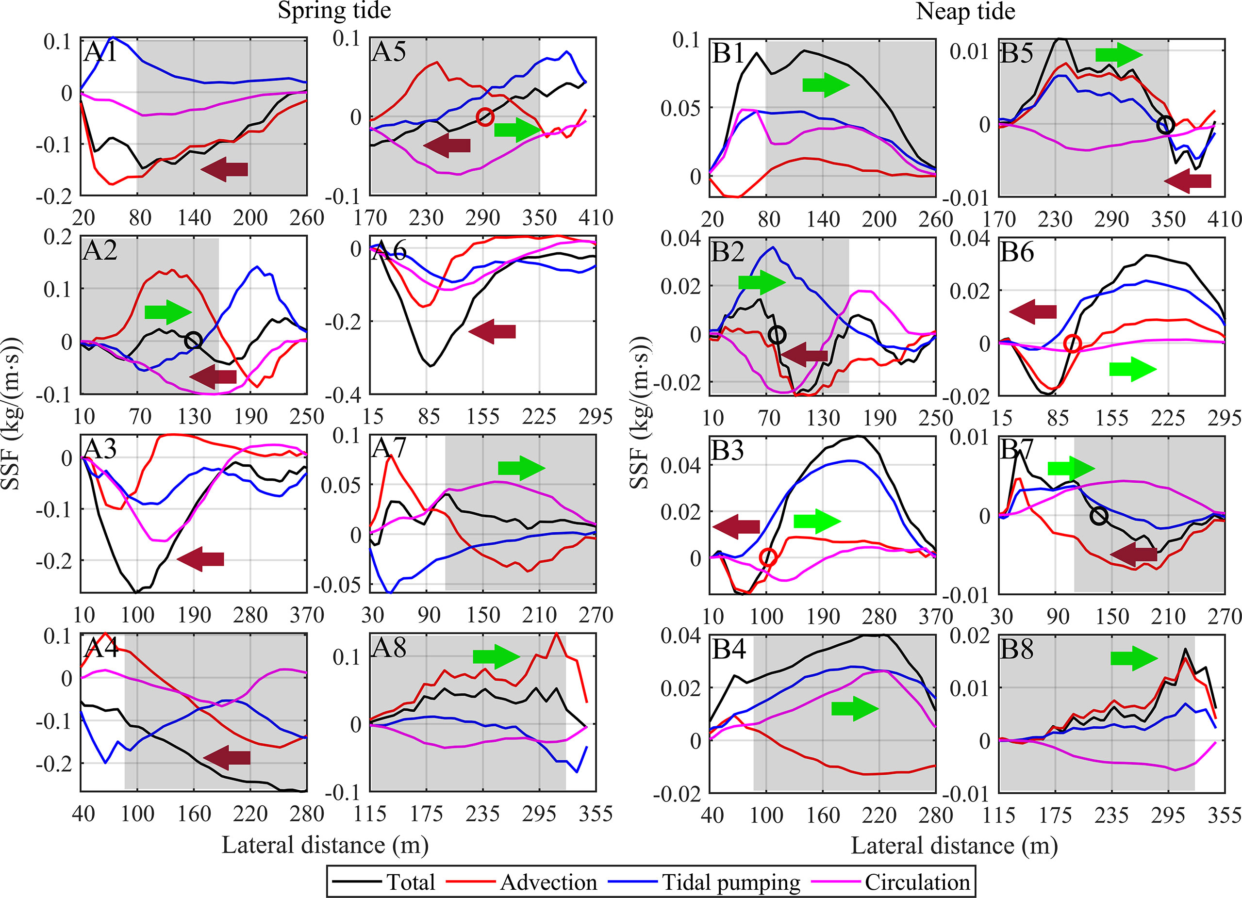
Figure 12 Distribution of lateral residual SSF and decomposition at eight transects during spring (A1–A8) and neap (B1–B8) tides. Positive values indicate transport toward the right bank, and the left origin denotes the left bank. Gray indicates the area between the deepest part of the channel and the convex bank side, i.e., the slope of the convex bank. Transects S3 and S6 are situated in the transition straight reaches; thus, no gray areas or convex bank exist here. Colored arrows indicate the direction of total sediment transport. Hollow black and red circles indicate convergence and divergence of the sediment transport, respectively. SSF, suspended sediment flux.
At transect S4, with the three-layer lateral circulation structure at spring tide (Figure 4B4), a stronger current directs toward the right bank in the middle layer. Driven by all three terms on the slope of the convex bank, sediment is mainly transported toward the right bank at spring tide (Figure 12A4), while at neap tide, circulation changes into the two-layer structure (Figure 4C4). The tidal pumping and circulation transport dominate the rightward transport (Figure 12B4), which is consistent with the bottom flow of the two-layer circulation. At transect S5 (Figure 12A5), the divergence of sediment transport occurs on the slope of the convex bank at spring tide, which is dominated by the circulation transport toward the shoal and by the tidal pumping toward the channel. At neap tide, the convergence of sediment transport occurs in the deepest part of the channel (Figure 12B5). It is dominated by the advection and tidal pumping transport toward the channel on the slope of the convex bank. However, the circulation transport is still toward the shoal, the same as that of spring tide. At transect S7 (Figure 12A7), circulation transport dominates the rightward transport toward the convex bank at spring tide. At neap tide, transport convergence emerges on the slope of the convex bank (Figure 12B7), which is driven by circulation transport toward the shoal and advection transport toward the channel. At transect S8, although the circulation transport is still toward the shoal, sediment is transported toward the channel at both spring and neap tides due to the advection-dominated transport (Figures 12A8, B8).
At transects S3 and S6 in the transition straight reaches, sediment is transported toward the left bank at spring tide (Figures 12A3, A6), even though the circulation transport presents the divergence pattern in the vicinity of the deep channel. At neap tide, both total transport and circulation transport show a divergence pattern in the channel (Figures 12B3, B6). Also, the divergence pattern of circulation transport that occurs at both spring and neap tides is consistent with the bottom flow direction of the double-cell circulation structure at transects in the transition straight reaches.
Although the dominant mechanisms of lateral sediment transport at various transects are different from each other, circulation transport plays an important role in lateral sediment transportation and trapping as described below (Section 5.3). The circulation transport is dependent on the bottom flow of the lateral circulation structure. It transports sediment toward the convex bank in the bend reaches, while in the transition straight reaches it presents the divergence pattern.
5.3 Sediment trapping mechanisms
The tidal pumping and circulation transport are the main driving mechanisms for landward sediment transport (Figure 11). At spring tide, the stronger tidal energy will generate larger landward transport by the tidal pumping, transporting the ETM upstream farther away from the estuary. While at neap tide, the weakening tidal energy reduces the tidal pumping transport. The exchange flow inside the estuary driven by the larger longitudinal density gradient will enhance the circulation transport and drive the sediment importation from the outer sea, but the ETM is closer to the estuary compared with the ones of spring tide.
At the river mouth bend, due to the total transport toward the left bank, the high-turbidity zone is slightly deflected to the channel at spring tide (Figures 4D1, 12A1). However, no obvious deflection occurs at neap tide because total transport shifts toward the right bank with opposite circulation structure (Figures 4E1, 12B1). The direction or convergence of the total transport tends to determine patterns of sediment trapping, i.e., the position that sediment will be trapped in, such as at transects S2, S4, and S7 (Figures 12A2, A7, B2, B4, B7). Here, sediment is trapped on the shoal of the convex bank by the circulation transport (Figures 4D2, D7, E2, E4, E7). The bottom flow of the circulation is toward the convex bank and moves sediment upslope toward the shoal, while advection and tidal pumping often transport sediment downslope toward the channel.
However, the trapping position is not always consistent with the direction of total transport. At transects S4, S5, and S8, circulation transport toward the convex bank is smaller than advection and tidal pumping toward the channel; thus, total transport is toward the deep channel on the slope of the convex bank (Figures 12A4, A5, A8, B5, B8). Nevertheless, sediment is still trapped on the shoal of the convex bank (Figures 4D4, D5, D8, E5, E8). Take transect S8 as an example, in the upper layer, sediments are transported toward the channel due to advection or tidal pumping. Its SSF per unit width over a tidal cycle is 18.929 t and 2.339 t toward the channel at spring and neap tides, respectively. In the bottom layer, the circulation transport moves sediment upslope to the convex bank, of which SSF is 14.468 and 1.810 t toward the shoal. It is smaller than that of the upper layer. Eventually, the total transport toward the channel is 4.460 and 0.529 t, respectively. Because transect S8 is located near the ETM at spring tide, the SSC is large in the whole water column. Also, during neap tide, the SSC is very small in the water column. Thus, the SSC in the upper layer is not much less than that of the lower layer. A stronger flow toward the channel causes a larger sediment transport in the upper layer. While in the lower layer, a large SSC leads to a considerable transport toward the shoal which is slightly smaller than that of the upper layer. Although the total sediment transport integrated over the depth is toward the channel (Figures 12A8, B8), the high turbidity at the bottom layer is still transported to the shoal (Figures 4D8, E8). Thus, the direction of bottom flow and circulation transport determine patterns of sediment trapping.
The lateral trapping of the suspended sediment on the shoal of the convex bank at the bend reaches is consistent with the direction of the bottom residual flow toward the convex bank and the circulation transport. In other words, the lateral flow will produce a strong lateral circulation transport, thereby redistributing bottom sediment along the cross section. In addition, the bottom lateral flow will determine the direction of sediment trapping. For bends, the prominent channel–shoal morphology, where the deep channel is located near the concave bank and the shoal is located near the convex bank, will generate the bottom residual current toward the shoal of the convex bank (Figures 4B8, C8), causing sediment to be laterally trapped there (Figures 4D8, E8). However, without the obvious channel–shoal morphology like bends, the symmetrical cross section in the transition straight reaches and divergence of the lateral residual current at the bottom and circulation (total) transport (Figures 4B3, B6, C3, C6) will not produce an obvious lateral trapping phenomenon. Thus, the high-turbidity zone is still located in the center of the deep channel (Figures 4D3, D6, E3, E6). Abundant sediment is trapped on the shoal of the convex bank in the bend reaches, which can cause severe siltation on the shoal (Figure 9). It is consistent with the present riverbed evolution trend in the YE, in that sediment deposition has been found widespread on the side shoal since 2001 (Zhao et al., 2015).
5.4 Limitations
The data set utilized in this paper is admittedly limited as it consists of only several tidal cycles. A longer temporal variation of the flow-sediment dynamics needs to be studied further. Combined with the observed data in the dry season, we can gain insight into the shift of the sediment trapping mechanisms with the various tidal ranges and river runoffs in different seasons in the future study. Also, only four-cross-section data are collected in the Yongjiang River, which is inadequate. Supplementary measurement of other typical cross sections will be conducted in the future to produce more in situ data support, drawing conclusions more reliably.
In the model, many hydraulic structures constructed in the YE (Yan, 2011) are not considered, which may affect the hydro and sediment dynamics to some extent. Furthermore, only one sediment fraction, cohesive mud, is included in the model. Improvement to the model would be to account for multiple suspended sediment fractions, flocculation, and hindered settling to calculate sediment settling velocity with spatial and temporal variation, which can result in distinctive sediment transport patterns (Winterwerp, 2002; Winterwerp, 2011; Yang et al., 2014). Other limitations include not considering the effect of sediment on fluid density, which has been confirmed to significantly shift the ETM dynamics in the Yangtze Estuary by the sediment-induced density gradient (Zhu et al., 2021), wind stress, and sediment resuspension by wind waves (Huijts et al., 2006).
Finally, an idealized or generalized model will be established in the future according to the basic data of the YE, in which various processes of the longitudinal and lateral sediment trapping will be analyzed by numerical tests of sensitivity with different flow-sediment conditions in the upper reaches of the estuary, tidal constituents in the outer sea, sediment fractions, and cross section shapes, aiming to provide support for theories of sediment trapping in other curved estuaries.
6 Conclusions
Based on the measured water and sediment data in the flood season and the results of the three-dimensional baroclinic flow and sediment numerical model, the spatial structure of the water and sediment dynamics in the YE and the spatial and temporal distribution characteristics of the ETM are analyzed. Also, mechanisms of the residual flow and sediment trapping are discovered according to the momentum balance analysis and sediment flux decomposing, respectively.
Results reveal that baroclinic effects are extremely important for both residual flow and sediment transport in the lower reaches. They drive the estuarine circulation and significantly shift the longitudinal/lateral momentum balance. The ETM during spring tides is generated by the landward tidal pumping, and longitudinally trapped in the upmost estuary. With the weakening of the tidal forcing, the location of the ETM is shifted to lower reaches closer to the sea mouth during neap tides, and it is dominated by the circulation transport. In the medium estuary such as the YE, the intratidal bidirectional transport of the ETM can be throughout the estuary during spring tides, which can cause severe deposition within the whole estuary.
The patterns of the lateral sediment trapping are different in the curved and straight reaches. The sediment at the curved reaches is laterally trapped on the shoal of the convex bank, caused by the circulation transport of which the direction is consistent with the bottom flow of the lateral circulation. Although the advection and tidal pumping transport tend to transport sediment downslope toward the channel and dominate total transport, the circulation transport determined by the bottom flow of the lateral circulation can move abundant sediment in the bottom layer upslope to the convex bank. Eventually, the sediment is trapped on the convex bank caused by the circulation transport and the bottom flow. In the transition straight reaches, the bottom divergent flow and circulation (total) transport cause the high-turbidity zone to be still located in the center of the deep channel, without any obvious lateral trapping phenomenon.
Data availability statement
The raw data supporting the conclusions of this article will be made available by the authors, without undue reservation.
Author contributions
JT acted as RZ supervisor in guiding the whole study, provided the in situ observed data, performed the results analysis, and revised the manuscript. RZ designed the modeling study, performed the data analysis, prepared the figures, and wrote the manuscript draft. All authors contributed to the article and approved the submitted version.
Funding
The work was funded by the National Natural Science Foundation of China (Grant No. 52071129).
Acknowledgments
The authors would like to thank two reviewers for constructive and helpful comments and the editor AS for handling the manuscript.
Conflict of interest
The authors declare that the research was conducted in the absence of any commercial or financial relationships that could be construed as a potential conflict of interest.
Publisher’s note
All claims expressed in this article are solely those of the authors and do not necessarily represent those of their affiliated organizations, or those of the publisher, the editors and the reviewers. Any product that may be evaluated in this article, or claim that may be made by its manufacturer, is not guaranteed or endorsed by the publisher.
References
Alahmed S., Ross L., Sottolichio A. (2021). The role of advection and density gradients in driving the residual circulation along a macrotidal and convergent estuary with non-idealized geometry. Cont. Shelf Res. 212, 104295. doi: 10.1016/j.csr.2020.104295
Allen G. P., Salomon J. C., Bassoullet P., Du Penhoat Y., de Grandpré C. (1980). Effects of tides on mixing and suspended sediment transport in macrotidal estuaries. Sediment. Geol. 26 (1), 69–90. doi: 10.1016/0037-0738(80)90006-8
Burchard H., Baumert H. (1998). The formation of estuarine turbidity maxima due to density effects in the salt wedge. a hydrodynamic process study. J. Phys. Oceanogr. 28 (2), 309–321. doi: 10.1175/1520-0485(1998)028<0309:TFOETM>2.0.CO;2
Burchard H., Schuttelaars H. M., Ralston D. K. (2018). Sediment trapping in estuaries. Annu. Rev. Mar. Sci. 10 (1), 371–395. doi: 10.1146/annurev-marine-010816-060535
Chernetsky A. S., Schuttelaars H. M., Talke S. A. (2010). The effect of tidal asymmetry and temporal settling lag on sediment trapping in tidal estuaries. Ocean Dyn. 60 (5), 1219–1241. doi: 10.1007/s10236-010-0329-8
De Jonge V. N., Schuttelaars H. M., van Beusekom J. E. E., Talke S. A., de Swart H. E. (2014). The influence of channel deepening on estuarine turbidity levels and dynamics, as exemplified by the ems estuary. Estuar. Coast. Shelf Sci. 139, 46–59. doi: 10.1016/j.ecss.2013.12.030
Deltares (2021) Delft3D-flow hydro-morphodynamics user manual. Available at: https://oss.deltares.nl/web/delft3d/.
De Nijs M. A. J., Winterwerp J. C., Pietrzak J. D. (2009). On harbour siltation in the fresh-salt water mixing region. Cont. Shelf Res. 29 (1), 175–193. doi: 10.1016/j.csr.2008.01.019
De Swart H. E., Schuttelaars H. M., Talke S. A. (2009). Initial growth of phytoplankton in turbid estuaries: A simple model. Cont. Shelf Res. 29 (1), 136–147. doi: 10.1016/j.csr.2007.09.006
Dyer K. R. (1986). Coastal and estuarine sediment dynamics Vol. 173 (England, Chichester: John Wiley & Sons Inc).
Dyer K. R. (1988). “Fine sediment particle transport in estuaries,” in Physical processes in estuaries. Eds. Dronkers J., van Leussen W. (Berlin, Heidelberg: Springer), 295–310.
Eidam E., Sutherland D. A., Ralston D. K., Conroy T., Dye B. (2021). Shifting sediment dynamics in the coos bay estuary in response to 150 years of modification. J. Geophys. Res.-Oceans 126, e2020JC016771. doi: 10.1029/2020JC016771
Fugate D. C., Friedrichs C. T., Sanford L. P. (2007). Lateral dynamics and associated transport of sediment in the upper reaches of a partially mixed estuary, Chesapeake bay. U.S.A. Cont. Shelf Res. 27 (5), 679–698. doi: 10.1016/j.csr.2006.11.012
Gao S. (2006). Catchment-coast interactions of the Asian region: APN recent research topics. Adv. Earth Sci. 21 (07), 680–686. doi: 10.3321/j.issn:1001-8166.2006.07.004
Garnier J., Billen G., Némery J., Sebilo M. (2010). Transformations of nutrients (N, p, Si) in the turbidity maximum zone of the seine estuary and export to the sea. Estuar. Coast. Shelf Sci. 90 (3), 129–141. doi: 10.1016/j.ecss.2010.07.012
Geyer W. R. (1993). The importance of suppression of turbulence by stratification on the estuarine turbidity maximum. Estuaries 16 (1), 113–125. doi: 10.2307/1352769
Geyer W. R., MacCready P. (2014). The estuarine circulation. Annu. Rev. Fluid Mech. 46, 175–197. doi: 10.1146/annurev-fluid-010313-141302
Geyer W. R., Signell R. P., Kineke G. C. (1998). “Lateral trapping of sediment in partially mixed estuary,” in Physics of estuaries and coastal seas. Ed. Dronker J., Scheffers M. (Netherlands, Rotterdam: A. A. Balkema), 115–124.
Geyer W. R., Woodruff J. D., Traykovski P. (2001). Sediment transport and trapping in the Hudson river estuary. Estuaries 24 (5), 670–679. doi: 10.2307/1352875
Glangeaud L. (1938). Transport of sedimentation chlans l estuare et l embouchure de la girronde. Bull. Soc Geol. Fr. 8 (3), 599–630.doi: 10670/1.tt2zs2
Grabemann I., Uncles R. J., Krause G., Stephens J. A. (1997). Behaviour of turbidity maxima in the Tamar (U.K.) and weser (F.R.G.). Estuaries. Estuar. Coast. Shelf Sci. 45 (2), 235–246. doi: 10.1006/ecss.1996.0178
He X., Wang Y. P., Zhu Q., Zhang Y., Zhang D., Zhang J., et al. (2015). Simulation of sedimentary dynamics in a small-scale estuary: The role of human activities. Environ. Earth Sci. 74 (1), 869–878. doi: 10.1007/s12665-015-4100-9
Holt J. T., James I. D. (1999). A simulation of the southern north Sea in comparison with measurements from the north Sea project part 2 suspended particulate matter. Cont. Shelf Res. 19 (12), 1617–1642. doi: 10.1016/S0278-4343(99)00032-1
Huijts K., Schuttelaars H. M., And H., Valle-Levinson A. (2006). Lateral entrapment of sediment in tidal estuaries: An idealized model study. J. Geophys. Res.-Oceans 111, C12016. doi: 10.1029/2006JC003615
Jalón-Rojas I., Dijkstra Y. M., Schuttelaars H. M., Brouwer R. L., Schmidt S., Sottolichio A. (2021). Multidecadal evolution of the turbidity maximum zone in a macrotidal river under climate and anthropogenic pressures. J. Geophys. Res.-Oceans 126 (5), e2020JC016273. doi: 10.1029/2020JC016273
Jay D. A., Dungan Smith J. (1990). Circulation, density distribution and neap-spring transitions in the Columbia river estuary. Prog. Oceanogr. 25 (1), 81–112. doi: 10.1016/0079-6611(90)90004-L
Jay D. A., Talke S. A., Hudson A., Twardowski M. (2015). “Estuarine turbidity maxima revisited: Instrumental approaches, remote sensing, modeling studies, and new directions,” in Fluvial-tidal sedimentology. Eds. Ashworth P. J., Parsons J. L. B. &D. R. (Amsterdam: Elsevier), 49–109.
Jones W. P., Launder B. (1972). The prediction of laminarization with a two-equation model of turbulence. Int. J. Heat Mass Transf. 15 (2), 301–314. doi: 10.1016/0017-9310(72)90076-2
Kuai Y., Tao J., Zhang Q., Zhang C. (2017). Numerical simulation on the tidal current and sediment for the yongjiang river and out sea area. Port Waterway Eng. 531 (07), 58–67. doi: 10.16233/j.cnki.issn1002-4972.2017.07.013
Le Hir P., Ficht A., Jacinto R. S., Lesueur P., Dupont J. P., Lafite R., et al. (2001). Fine sediment transport and accumulations at the mouth of the seine estuary (France). Estuaries 24 (6B), 950–963. doi: 10.2307/1353009
Lerczak J. A., Geyer W. R. (2004). Modeling the lateral circulation in straight, stratified estuaries*. J. Phys. Oceanogr. 34 (6), 1410–1428. doi: 10.1175/1520-0485(2004)034<1410:MTLCIS>2.0.CO;2
Leuven J. R. F. W., Pierik H. J., Vegt M., Bouma T. J., Kleinhans M. G. (2019). Sea-Level-rise-induced threats depend on the size of tide-influenced estuaries worldwide. Nat. Clim. Change 9 (12), 986–992. doi: 10.1038/s41558-019-0608-4
Little S., Spencer K. L., Schuttelaars H. M., Millward G. E., Elliott M. (2017). Unbounded boundaries and shifting baselines: Estuaries and coastal seas in a rapidly changing world. Estuar. Coast. Shelf Sci. 198, 311–319. doi: 10.1016/j.ecss.2017.10.010
Liu W.-C., Hsu M.-H., Kuo A. Y. (2002). Modelling of hydrodynamics and cohesive sediment transport in tanshui river estuarine system, Taiwan. Mar. pollut. Bull. 44 (10), 1076–1088. doi: 10.1016/S0025-326X(02)00160-1
Li X., Zhu J., Yuan R., Qiu C., Wu H. (2016). Sediment trapping in the changjiang estuary: Observations in the north passage over a spring-neap tidal cycle. Estuar. Coast. Shelf Sci. 177, 8–19. doi: 10.1016/j.ecss.2016.05.004
MacCready P., Geyer W. R. (2010). Advances in estuarine physics. Annu. Rev. Mar. Sci. 2, 35–58. doi: 10.1146/annurev-marine-120308-081015
Mariotti G., Fagherazzi S. (2012). Channels-tidal flat sediment exchange: The channel spillover mechanism. J. Geophys. Res.-Oceans 117 (C3), C03032. doi: 10.1029/2011jc007378
McSweeney J. M., Chant R. J., Sommerfield C. K. (2016). Lateral variability of sediment transport in the Delaware estuary. J. Geophys. Res.-Oceans 121 (1), 725–744. doi: 10.1002/2015jc010974
Milliman J. D., Farnsworth K. L. (2011). River discharge to the coastal ocean: A global synthesis (Cambridge, New York: Cambridge University Press).
Orseau S., Lesourd S., Huybrechts N., Gardel A. (2017). Hydro-sedimentary processes of a shallow tropical estuary under Amazon influence. the mahury estuary, French Guiana. Estuar. Coast. Shelf Sci. 189, 252–266. doi: 10.1016/j.ecss.2017.01.011
Partheniades E. A. (1965). Erosion and deposition of cohesive soils. J. Hydraulic Division 91 (1), 105–139. doi: 10.1061/JYCEAJ.0001461
Ralston D. K., Geyer W. R., Warner J. C. (2012). Bathymetric controls on sediment transport in the Hudson river estuary: Lateral asymmetry and frontal trapping. J. Geophys. Res.-Oceans 117, C10013. doi: 10.1029/2012jc008124
Robinson I. S. (1983). “Tidally induced residual flows,” in Physical oceanography of coastal and shelf seas. Ed. Johns B. (Netherlands, Amsterdam: Elsevier), 321–356.
Schoellhamer D. H. (2000). “Influence of salinity, bottom topography, and tides on locations of estuarine turbidity maxima in northern San Francisco bay,” in Proceedings in marine science. Eds. McAnally W. H., Mehta A. J. (Netherlands, Amsterdam: Elsevier), 343–357.
Schubel J. R. (1968). Turbidity maximum of the northern chesapeake bay. Science 161 (3845), 1013–1015. doi: 10.1126/science.161.3845.1013
Sommerfield C. K., Wong K.-C. (2011). Mechanisms of sediment flux and turbidity maintenance in the Delaware estuary. J. Geophys. Res.-Oceans 116 (C1), C01005. doi: 10.1029/2010JC006462
Stelling G. S., Van Kester J. A. T. M. (1994). On the approximation of horizontal gradients in sigma co-ordinates for bathymetry with steep bottom slopes. Int. J. Numer. Methods Fluids 18 (10), 915–935. doi: 10.1002/fld.1650181003
Uncles R. J., Elliott R. C. A., Weston S. A. (1985). Dispersion of salt and suspended sediment in a partly mixed estuary. Estuaries 8 (3), 256–269. doi: 10.2307/1351486
Uncles R. J., Stephens J. A., Law D. J. (2006). Turbidity maximum in the macrotidal, highly turbid Humber estuary, UK: Flocs, fluid mud, stationary suspensions and tidal bores. Estuar. Coast. Shelf Sci. 67 (1), 30–52. doi: 10.1016/j.ecss.2005.10.013
Wai O. W. H., Wang C. H., Li Y. S., Li X. D. (2004). The formation mechanisms of turbidity maximum in the pearl river estuary. China. Mar. pollut. Bull. 48 (5-6), 441–448. doi: 10.1016/j.marpolbul.2003.08.019
Wan X., Li J., Shen H. (2009). Distribution and fluxes of suspended sediments in the offshore waters of the changjiang (yangtze) estuary. Acta Oceanol. Sin. 28 (4), 86–95. doi: 10.3969/j.issn.0253-505X.2009.04.012
Winterwerp J. C. (2002). On the flocculation and settling velocity of estuarine mud. Cont. Shelf Res. 22 (9), 1339–1360. doi: 10.1016/S0278-4343(02)00010-9
Winterwerp J. C. (2011). Fine sediment transport by tidal asymmetry in the high-concentrated ems river: indications for a regime shift in response to channel deepening. Ocean Dyn. 61 (2), 203–215. doi: 10.1007/s10236-010-0332-0
Winterwerp J. C., Zhou Z., Battista G., Van Kessel T., Jagers H. R. A., Van Maren D. S., et al. (2018). Efficient consolidation model for morphodynamic simulations in low-SPM environments. J. Hydraul. Eng.-ASCE 144 (8), 04018055. doi: 10.1061/(ASCE)HY.1943-7900.0001477
Xiao Y., Wu Z., Cai H., Tang H. (2018). Suspended sediment dynamics in a well-mixed estuary: The role of high suspended sediment concentration (SSC) from the adjacent sea area. Estuar. Coast. Shelf Sci. 209, 191–204. doi: 10.1016/j.ecss.2018.05.018
Xie D., Pan C., Wu X., Gao S., Wang Z. (2017). The variations of sediment transport patterns in the outer changjiang estuary and hangzhou bay over the last 30 years. J. Geophys. Res.-Oceans 122 (4), 2999–3020. doi: 10.1002/2016JC012264
Yan W. (2011). Water and sediment characteristics and their scouring and silting law in the three rivers of ningbo. Hydro-Science Eng. 04, 143–148. doi: 10.3969/j.issn.1009-640X.2011.04.023
Yang Z., de Swart H. E., Cheng H., Jiang C., Valle-Levinson A. (2014). Modelling lateral entrapment of suspended sediment in estuaries: The role of spatial lags in settling and m-4 tidal flow. Cont. Shelf Res. 85, 126–142. doi: 10.1016/j.csr.2014.06.005
Yellen B., Woodruff J. D., Ralston D. K., MacDonald D. G., Jones D. S. (2017). Salt wedge dynamics lead to enhanced sediment trapping within side embayments in high-energy estuaries. J. Geophys. Res.-Oceans 122 (3), 2226–2242. doi: 10.1002/2016JC012595
Zhang S., Mao X.-z. (2015). Hydrology, sediment circulation and long-term morphological changes in highly urbanized shenzhen river estuary, China: A combined field experimental and modeling approach. J. Hydrol. 529, 1562–1577. doi: 10.1016/j.jhydrol.2015.08.027
Zhao C., Wang L., Yu D. (2015). The influence of desilting engineering on flood control and drainage in tidal river network area and study on engineering proposal. J. Water Resour. Res. 2), 199. doi: 10.12677/jwrr.2015.42023
Zhou Z., Ge J., van Maren D. S., Wang Z. B., Kuai Y., Ding P. X. (2021). Study of sediment transport in a tidal channel-shoal system: lateral effects and slack-water dynamics. J. Geophys. Res.-Oceans 126 (3), e2020JC016334. doi: 10.1029/2020JC016334
Zhou Z., Ge J., Wang Z. B., van Maren D. S., Ma J., Ding P. (2019). Study of lateral flow in a stratified tidal channel-shoal system: the importance of intratidal salinity variation. J. Geophys. Res.-Oceans 124 (9), 6702–6719. doi: 10.1029/2019JC015307
Zhou J., Stacey M. T. (2020). Residual sediment transport in tidally energetic estuarine channels with lateral bathymetric variation. J. Geophys. Res.-Oceans 125, e2020JC016140. doi: 10.1029/2020JC016140
Zhou J., Stacey M. T., Holleman R. C., Nuss E., Senn D. B. (2020). Numerical investigation of baroclinic channel-shoal interaction in partially stratified estuaries. J. Geophys. Res.-Oceans 125 (10), e2020JC016140. doi: 10.1029/2020JC016135
Keywords: residual current, estuarine turbidity maximum, lateral dynamics, momentum balance analysis, sediment trapping, curved estuary
Citation: Tao J and Zhu R (2022) Exploring the three-dimensional flow-sediment dynamics and trapping mechanisms in a curved estuary: The role of salinity and circulation. Front. Mar. Sci. 9:976332. doi: 10.3389/fmars.2022.976332
Received: 23 June 2022; Accepted: 03 August 2022;
Published: 05 September 2022.
Edited by:
Zhan Hu, Sun Yat-sen University, Zhuhai Campus, ChinaCopyright © 2022 Tao and Zhu. This is an open-access article distributed under the terms of the Creative Commons Attribution License (CC BY). The use, distribution or reproduction in other forums is permitted, provided the original author(s) and the copyright owner(s) are credited and that the original publication in this journal is cited, in accordance with accepted academic practice. No use, distribution or reproduction is permitted which does not comply with these terms.
*Correspondence: Renjie Zhu, MjAxMzAzMDIwMDU4QGhodS5lZHUuY24=