A lens-shaped, cold-core anticyclonic surface eddy in the northern South China Sea

Typically, compared with the normal ocean, an anticyclonic eddy has higher sea surface temperature (SST), greater surface mixed-layer depth (MLD), and a bowl-shaped structure under the action of geostrophy. This study is the first to report an abnormal anticyclonic eddy characterized by a lens-shaped structure, cold core, and shallower MLD, which were observed in situ in the northern South China Sea (SCS) in September 2021. The SST at core of the anticyclonic eddy was 0.4°C lower than that in its peripheral region. The MLD at the center of the eddy was about half of that outside the eddy. Below the surface mixed layer, a lens-shaped structure containing relatively well-mixed water was observed between the two high-gradient layers. Within this lens-shaped structure, the isothermal layers were stretched, but accompanied by water mixing that was about one third of that at the upper and lower bounds of the structure. This eddy originated from a Kuroshio Current intrusion in late October 2020 and died in November 2021, such that its lifespan exceeded 1 year. The shedding of the Kuroshio Loop into the SCS under strong air–sea interactions under continuous sea surface cooling in winter was considered a key mechanism for the generation of the cold core of the eddy. The lens-shaped structure formed below the surface mixed layer and was maintained through geostrophic balance by the subsurface maximum speeds of the Kuroshio Current intrusion (50–100 m), thereby forming a shallower MLD in the eddy center. The subsurface speed maximum within the eddy was also observed by a shipborne acoustic Doppler current profiler at 10 months after its formation, confirming the hypothesized mechanism. This type of abnormal anticyclonic may be a common phenomenon in the northern SCS and has potential implications for the local biogeochemistry, local heat budget, and regional oceanic models.

1 Introduction

Mesoscale eddies, with horizontal scales on the order of 100 km (Chelton et al., 2011a), are among the most significant features of the global ocean; they contain approximately 90% of the total kinetic energy of the world’s oceans (Ferrari and Wunsch, 2009). They have a strong impact on ocean circulation and climate through transporting and stirring momentum and tracers such as heat, salinity, and carbon dioxide along the density surface (Bryden and Brady, 1989; McGillicuddy et al., 2007; Dong et al., 2014; Zhang et al., 2014; Qiu et al., 2021, 2022).

Mesoscale eddies can be classified into two types based on their polarity, cyclonic and anticyclonic, each of which has different effects on sea surface temperature (SST). Cyclonic (anticyclonic) mesoscale eddies correspond to low (high) sea surface height (SSH), promoting sea surface divergence (convergence) under the action of geostrophy, resulting in the increase (fall) of lower (upper) sea water and leading to lower (higher) SSTs. Therefore, mesoscale eddies can be divided into cold and warm eddies, corresponding to cyclonic and anticyclonic eddies, respectively. These eddies can also alter the vertical structure of the ocean, such as the surface mixed layer (SML) (Hausmann et al., 2017; Gaube et al., 2019), which is deepened through anticyclonic eddy downwelling and shoaled through cyclonic eddy upwelling (Gaube et al., 2019). They produce physical and ecological characteristics on the sea surface that differ from the surrounding ocean; therefore, they can be detected in altimetric SSH images (Chelton et al., 2007; Chelton et al., 2011a; Faghmous et al., 2015), infrared/microwave SST images (Castellani, 2006; Isern-Fontanet et al., 2006; Dong et al., 2011), and sea surface chlorophyll maps (Chelton et al., 2011b; Gaube et al., 2014; Wang et al., 2018; Xu et al., 2019; Yang et al., 2020; Zhang & Qiu, 2020).

Abnormal eddies include anticyclonic cold-core eddies (ACEs) and cyclonic warm-core eddies (CWEs); their characteristics are the opposite of those of normal eddies. Abnormal eddies are common ocean phenomena that have been observed in many regional oceans, such as the South China Sea (SCS) (Liu et al., 2020; Sun et al., 2021), the North Pacific (Itoh and Yasuda, 2010; Sun et al., 2019), the Brazil–Malvinas Confluence Zone (Leyba et al., 2017), the Canada Basin, the Arctic Ocean (Timmermans et al., 2008), and the Bay of Bengal (Yang et al., 2020). One study reported that in the Tasman Sea, up to 44% of mesoscale eddies are CWEs, and 22% were ACEs (Everett et al., 2012). Abnormal eddies were found to account for approximately one third of all total mesoscale eddies in the global ocean using a combination of historical SSH and temperature data with deep learning (Liu et al., 2021). Like normal eddies, abnormal eddies have significant impacts on mass transport (Mathis et al., 2007; Everett et al., 2012), air–sea interactions (Leyba et al., 2017; Liu et al., 2020), and ocean circulation (Shimizu et al., 2001).

Previous studies have reported that the generation mechanisms of abnormal eddies include strong mixing (Martin and Richards, 2001), interaction between different water masses (Rabinovich et al., 2002), instability processes (Pickart et al., 2005; Spall et al., 2008; Kadko et al., 2008; Sun et al., 2019), eddy–wind interactions (McGillicuddy, 2015), Kuroshio Current intrusions (Sun et al., 2021), and changes in upper ocean stratification (He et al., 2020). For example, Martin and Richards (2001) revealed that an ACE formed from mode water created by deep winter mixing in the Iceland Basin region. Rabinovich et al. (2002) observed that an ACE was generated near Bussol Strait and intensified with the supply of cold freshwater from the Okhotsk Sea. Sun et al. (2021) studied abnormal eddies in the north Pacific Ocean and discussed two possible generation mechanisms, instability that dramatically changed the radius of a normal cyclonic eddy and absorbed warm sea water during the eddy decaying stage, and interaction between adjacent eddies that transported warm water into the surrounding area and entrained cold water into the interior of the anticyclonic eddy. McGillicuddy (2015) used numerical simulations to examine how eddy wind-driven upwelling (i.e., Ekman pumping) in anticyclones can yield a convex lens reminiscent of an ACE (a mode water eddy), whereas eddy wind-driven downwelling in cyclones produces an ACE. He et al. (2020) suggested that decreased sea surface salinity (SSS) resulted in changes in upper ocean stratification due to air–sea interactions in winter, and may also have formed ACEs in the Bay of Bengal in the India Ocean.

The SCS is a hotspot for energetic mesoscale eddy activity. On average, models have predicted approximately 33 eddies in the SCS every year that were verified by satellite data from 1993 to 2007 (Xiu et al., 2010). Recently, Sun et al. (2021) reported that abnormal eddies account for approximately 15% of all eddies in the SCS, based on model data. However, only a few studies have concentrated on abnormal eddies in the SCS, and no field observations have been conducted. The internal structural characteristics of abnormal eddies including temperature, salinity, size, influence depth, and generation mechanism have not been elucidated through field observations. Kuroshio Current intrusions are thought to be a key mechanism for abnormal eddy generation in the northeastern SCS (Sun et al., 2021). However, the factors influencing this process remain unknown. Therefore, in the present study, we examined the spatial characteristics of an ACE through in situ observations. The ACE formed in the Luzon Strait, with a life cycle of > 1 year and movement distance of >1000 km. Then, we evaluated the key dynamic factors that formed the ACE and maintained its cold core throughout its lifespan.

The remainder of this paper is organized as follows. Section 2 describes the field observations and auxiliary data used in this study, including remotely sensed satellite data and climatological data. Section 3 presents the characteristics of the ACE according to the in situ observation data. Section 4 discusses the possible generation mechanisms of the ACE. Section 5 presents our conclusions.

2 Data

2.1 In situ observations

Measurements were conducted in the northern SCS from 7 to 9 September 2021. The main objective of these observations was to investigate the temperature, salinity, and flow field structure of an anticyclonic eddy in the northern SCS. A total of 11 stations were positioned throughout the study area (Figure 1), which were grouped into two transects, latitudinal transect S1 (7 stations) and longitudinal transect S2 (5 stations, middle station taken in S1). Observations at transect S1 were conducted from 7 to 8 September, and those at transect S2 were conducted in 9 September. Detail information about the stations, such as observation time, latitude/longitude, water depths, and maximum depth of profile, is given in Table 1.

FIGURE 1

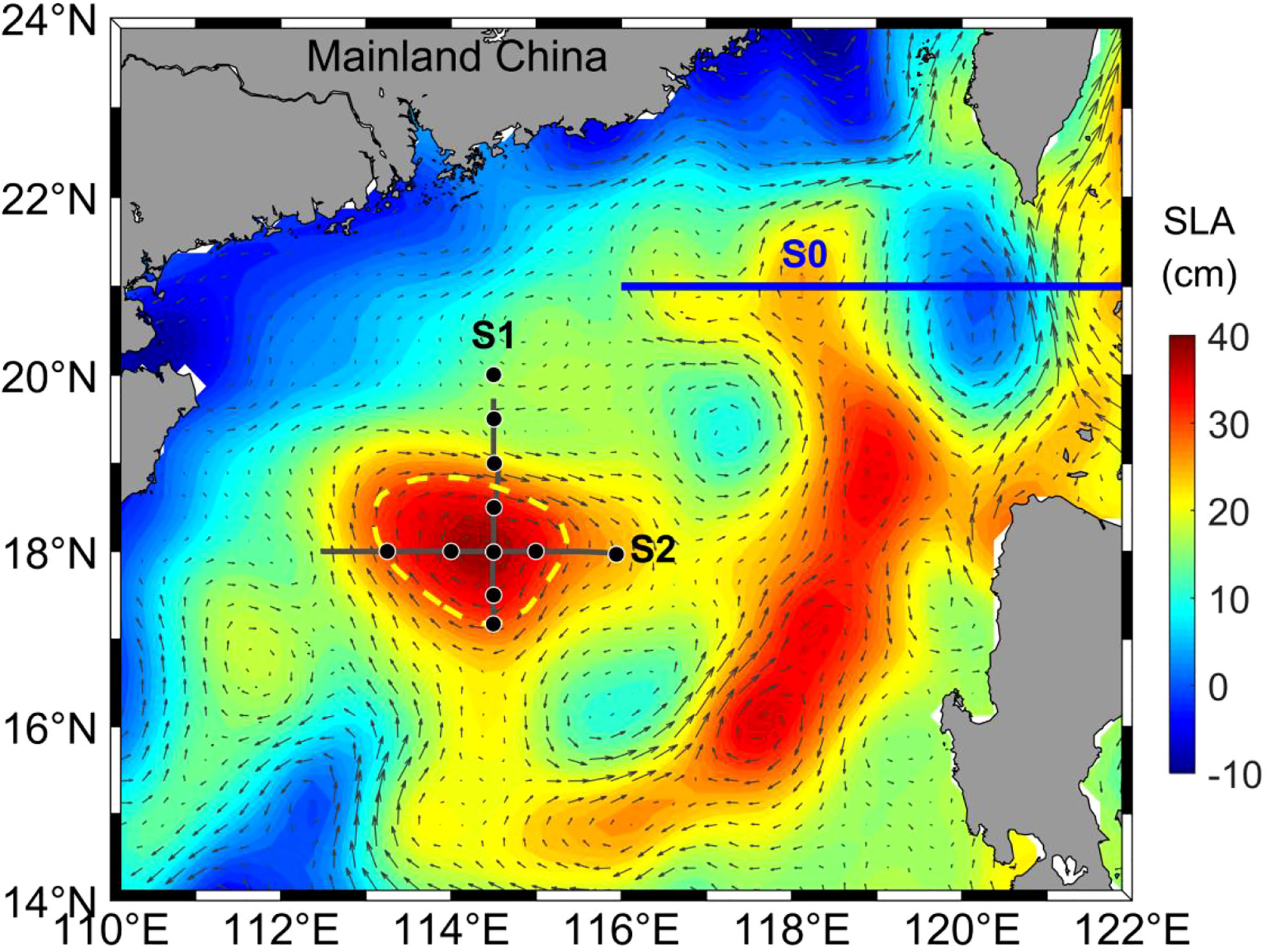
Figure 1 Sea level anomaly (SLA) and surface geostrophic flow in the South China Sea (SCS) on 8 September, 2021. The SLA data were produced by SSALTO/DUACS and distributed by Archiving, Validation and Interpretation of Satellite Oceanographic data (AVISO), with support from the Centre national d’études spatiales. Green dots indicate fine-scale electrical conductivity, temperature, and depth (CTD) observation locations; black dashed line indicates the anticyclonic eddy; green line indicates the zonal transect (S0) used to calculate geostrophic velocity in Section 4.2.

TABLE 1

Table 1 Information of the stations in this study.

An electrical conductivity, temperature, and depth (CTD) instrument (SBE 911plus; Sea-Bird Scientific, Philomath, OR, USA) was used to collect fine-scale temperature and salinity data. Accuracy of temperature and conductivity sensors are ±0.001°C and ±0.0003S/m, respectively. The CTD data were processed as recommended by the instrument manufacturer, and the bin was averaged to 1 m resolution. A shipborne broadband acoustic Doppler current profiler (ADCP; 150 kHz; Teledyne RD Instruments, Poway, CA, USA) operated continuously during the cruise, providing velocity information for the water column in the upper layer from surface to approximately 200 m depth. A bin size of 8 m and sampling interval of 1 min were adopted for the shipboard ADCP. Thus, the instrument captured one sample per minute.

2.2 Satellite data and climatological data

To examine the surface characteristics of the studied anticyclonic eddy, we obtained satellite altimeter-based sea level anomaly (SLA) data distributed by the Copernicus Marine Environment Monitoring Service (CMEMS, http://marine.copernicus.eu). The SLA dataset merged observations from different altimetry satellites (Jason-3, Sentinel-3A, HY-2A, Saral/AltiKa, Cryosat-2, Jason-2, Jason-1, T/P, ENVISAT, GFO, and ERS1/2), and corrected them geophysically and meteorologically for tides, ionospheric effects, and atmospheric pressure at gridded spatial and temporal resolutions of 1/4° and 1 day, respectively. The SLA data represent differences between absolute dynamic topography (ADT) and mean dynamic topography (MDT). The specific product used was SEALEVEL_GLO_PHY_L4_REP_OBSERVATIONS_008_046; a full description of the dataset is available at http://cmems-resources.cls.fr/documents/PUM/CMEMS-SL-PUM-008-032-051.pdf.

In addition to the SLA data, we obtained SST data collected by the Moderate Resolution Imaging Spectroradiometer (MODIS) from the National Aeronautics and Space Administration (NASA) OceanColor website (http://oceancolor.gsfc.nasa.gov). The MODIS-derived SST data used in this study were level-3, 8-day composite products with a spatial resolution of 4 km.

Climatological temperature and salinity fields were obtained from the World Ocean Atlas 2001 (http://apdrc.soest.hawaii.edu/data/data.php), at a spatial resolution of 0.25° × 0.25°. These data were used to calculate the geostrophic flow at transect S0 (Figure 1), with 1,000 m selected as the reference level.

The Archiving, Validation and Interpretation of Satellite Oceanographic data (AVISO) Mesoscale Eddy Trajectory Atlas product was used to display the moving path of the mesoscale eddy (https://www.aviso.altimetry.fr). The data processing methods used in constructing this dataset are described in detail elsewhere (Chelton et al., 2011a).

Historical temperature and salinity data from the Argo dataset (http://argo.ucsd.edu) were used to identify the origin of the eddy.

Winter sea surface wind data (January) were obtained from climatological sea surface wind data from a blended wind dataset (Zhang et al., 2006). These blended wind data combine multiple satellite observations and were used to fill data gaps in both time and space (https://www.ncei.noaa.gov/products/blended-sea-winds).

3 Results

3.1 Water mass characteristics of the ACE

The vessel sufficiently transited the center of the anticyclonic eddy (Figure 1) to study its structure. Vertical distributions of potential temperature (θ), salinity (S), potential density (σ_θ), and stratification (N²) are shown for both transects in Figure 2. The stratification, or squared buoyancy frequency, was calculated as,

$$N^2=–g/\rho \bullet \partial \rho /\partial z$$

FIGURE 2

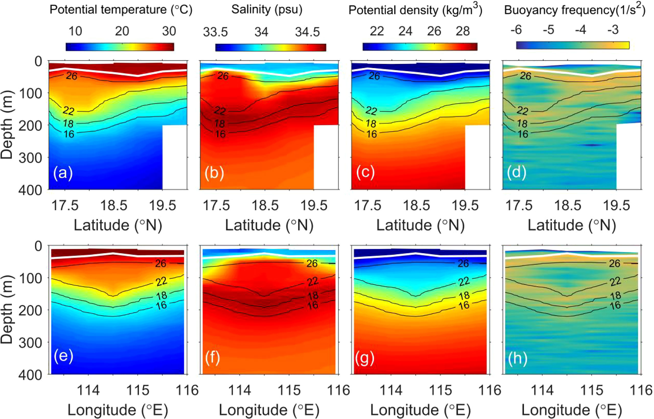
Figure 2 Distributions of thermohaline properties on transects S1 (top row) and S2 (bottom row), including (A, E) potential temperature, (B, F) salinity, (C, G) potential density, and (D, H) squared buoyancy frequency (N²). Grey lines indicate the mixed-layer depth (MLD). Isotherms of 26°C, 22°C, 18°C, and 16°C are indicated.

where g is the acceleration due to gravity and ρ is the density. In a normal anticyclonic eddy, we intuitively expect high SSTs, deeper mixed-layer depth (MLD), and a bowl-shaped temperature distribution (Frenger et al., 2015). However, the anticyclonic eddy observed in this study exhibited abnormal features including a lens-shaped core structure, MLD shoaling, and lower SSTs. These abnormal features also differ from those observed in a region near the study area in 2020 (Qi et al., 2021).

The main abnormal feature of the studied mesoscale eddy was its peculiar lens-shaped structure beneath the sea surface. This lens of relatively well-mixed water was squeezed between the two high-gradient layers that defined its upper and lower bounds (Lin et al., 2017). On transect S1, the lens-shaped structure was clearly observed at a vertical depth of approximately 25–150 m, between the 26°C and 22°C isotherms. The depth of the 26°C isotherm was approximately 40 m at the eddy core and approximately 60 m at the edge. By contrast, the depth of the 22°C isotherm was 150 m at the core and 90 m at the edge. Thus, the depth difference between the 26°C and 22°C isotherms increased from 30 m at the edge to 110 m at the eddy core. The horizontal extent of the lens was >160 km. This lens-shaped structure also had distinct vertical buoyancy frequency characteristics. Two high-gradient layers lay at the 26°C and 22°C isotherm depths (Figures 2D, H). The buoyancy frequency was two orders larger in these high-gradient layers than within the lens-shaped structure, where the isotherms and isosalinity lines appeared stretched, showing a low-gradient layer with low buoyancy frequency. By contrast, at the upper and lower boundaries of the structure, isotherms and isosalinity lines appeared compressed, showing a high-gradient layer with high buoyancy frequency. In the ocean thermocline, isotherm stretching is often accompanied by strong water mixing, such that well-mixed water is often detected between stretched isotherms (Dillon, 1982; Qi et al., 2020). In this study, the lens-shaped structure did not contain well-mixed water, but calm water with a dissipation rate and diffusivity that were much smaller than those of the surrounding water (Section 3.3). The same lens-shaped structure was also observed on the transect S2.

Lens-shaped subsurface anticyclonic eddies have been observed worldwide (Zhang et al., 2017; McCoy et al., 2020). The center of these lens-shaped subsurface eddies is usually located within or even below the main thermocline; thus, a considerable proportion of subsurface eddies are difficult to detect using satellite imagery because they lack strong surface signals. Lens-shaped subsurface eddies have previously been detected in the southern SCS, generated through the mixture of local mixed-layer water and water from Vietnam coastal jet separation (Lin et al., 2017). The lens-shaped structure within the core of the anticyclonic eddy examined in this study was not classified as a subsurface eddy due to its clear positive SLA signal (Figure 1), as well as its origin and development (Section 4). To the best of our knowledge, this study is the first to document a lens-shaped structure within a surface eddy.

The second abnormal feature of the mesoscale anticyclonic eddy examined in this study is MLD shoaling. Here, the MLD was identified as the depth at which the potential temperature varied by less than 0.5°C. The surface mixed layer (SML) is the conduit by which the atmosphere influences the ocean interior. Previous studies have reported that the MLD is deeper in anticyclonic eddies and shallower in cyclonic eddies (Williams, 1988; Gaube et al., 2019; Qi et al., 2021) due to the convergence and accumulation of warm water at the center of anticyclonic eddies; divergence at the center of cyclonic eddies cause upwelling of deep cold water. In this anticyclonic eddy, the MLD of the core was much smaller than that outside the eddy. On transect S1, the minimum MLD within the eddy was only 25 m, whereas the maximum MLD outside the eddy reached 48 m (Figure 3). A similar MLD pattern was also recorded on transect S2, with a minimum MLD within the eddy of 25 m and a maximum MLD outside the eddy of 40 m. To the best of our knowledge, this substantial MLD shoaling within an anticyclonic eddy has not been reported previously.

FIGURE 3

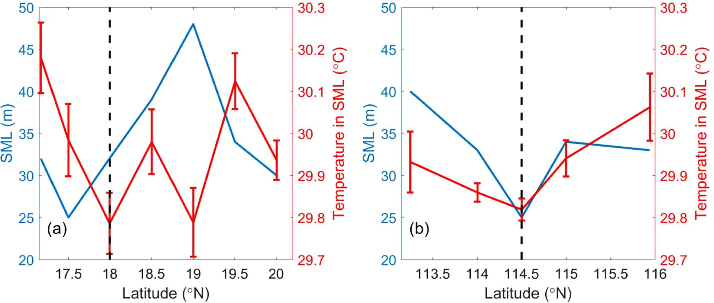
Figure 3 Distributions of surface mixed layer (SML) depth and its average temperature on transects (A) S1 and (B) S2. Black dash indicates the eddy center inferred from SLA data. Error bars indicate the standard deviation of temperature in SML at each station.

The interior of the anticyclonic eddy was also characterized by low SSTs. As a result of the well-mixed water within the SML, we used averaged temperature in the SML to represent this abnormal feature. On transect S1, the lowest averaged temperature within the SML was 29.8°C at the core of the eddy, which increased to 30.2°C at the left edge of eddy and 30.1°C at the right edge (Figure 3). Similar spatial distribution of temperatures was also observed on transect S2. Temperature within the SML can be affected by solar radiation (Liang et al., 2017), which rises toward noon and falls at night. In this study, observations at each transect were completed within 1 days, at a sampling interval of 4 h. Observations of the eddy core were recorded at noon and in the morning on transects S1 and S2, respectively, such that lower SSTs observed at core of the anticyclonic eddy were not caused by solar radiation. The lower SSTs within the anticyclonic eddy were validated by infrared SST images (Figure 4). Figure 4 shows distributions of MODIS 8-day (5–13 September 2021) composite 4 km SSTs. During this period, abnormally low SSTs were observed within the eddy. Although the feature of lower SSTs within the eddy was not obvious, it can be clearly shown in other periods (section 3.4). Remotely sensed SSTs were consistent with on-site CTD measurements (Figures 3, 4).

FIGURE 4

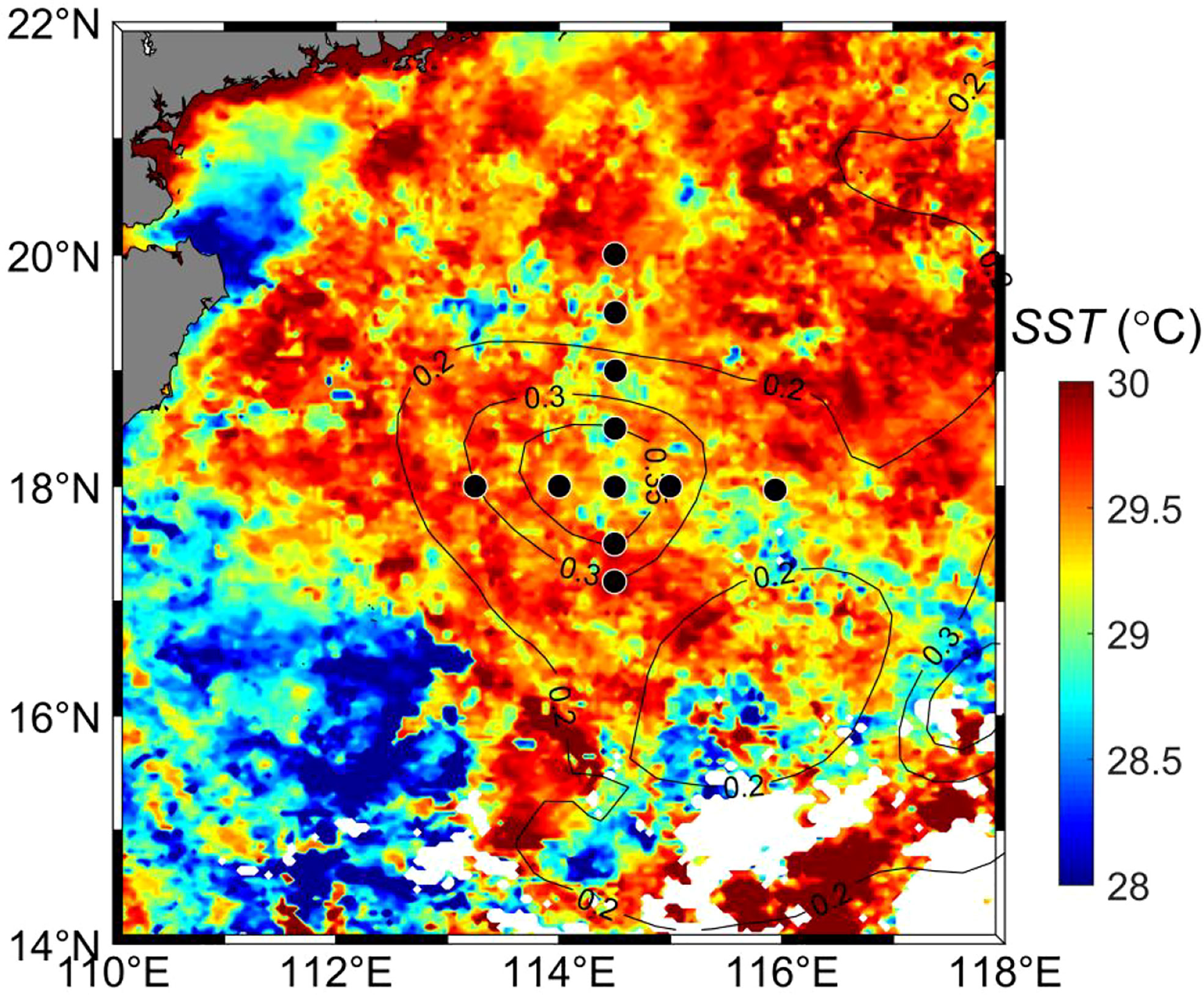
Figure 4 Maps of Moderate Resolution Imaging Spectroradiometer (MODIS) 8-day composite SSTs in the northeastern SCS recorded from 5to 13 September, 2021. White areas indicate poor data retrieval due to clouds. Black lines indicate 0.2, 0.3 and 0.35 m contours of the 8-day-averaged SLA during the same period. Black dots indicate measurement stations.

3.2 Flow field structure of the ACE

Depth profiles of the zonal velocity u, meridional velocity v, shear variance S², and Richardson number are shown in Figures 5A–D. This first layer of velocity lay at a depth of 14 m. The zonal velocity measured with the shipborne ADCP displayed obvious eddy structure characteristics, with northward flow to the left side of the anticyclonic eddy and southward flow to the right, eastward flow to the north and westward flow to the south (Figures 5A, F). Strong currents were detected within the lens‐shaped structure (Figures 5A, B, E, F). Notably, both zonal and meridional velocities within the lens-shaped structure were higher than those outside it. Within the lens-shaped structure, the maximum absolute zonal and meridional velocities were >0.5 m/s at a depth of 90 m, which corresponds to the vertical center. The currents decreased vertically to both sides, i.e., the velocity decreased as depth increased at >90 m and velocity decreased as depth decreased at<90 m. This vertical velocity distribution differed from the surrounding ocean, where currents typically decrease from the surface downward, and also from that of a normal surface anticyclonic eddy (Qi et al., 2021; Evans et al., 2022).

FIGURE 5

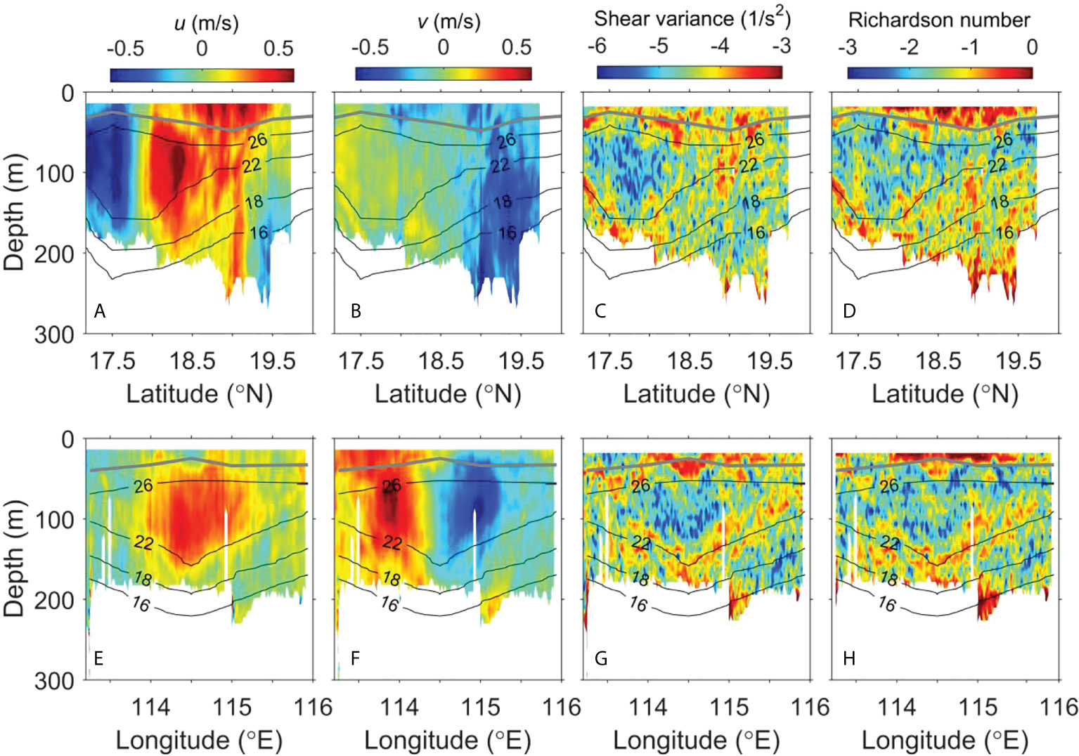
Figure 5 Flow field distributions on transects S1 (top row) and S2 (bottom row) for (A, E) zonal velocity u and (B, F) meridional velocity v, and log-transformed (C, G) shear variance [log₁₀(S)²] and (D, H) Richardson number [log₁₀(Ri^–1/4)]. Grey lines indicate the MLD. Isotherms of 26°C, 22°C, 18°C, and 16°C are indicated.

Above and below the lens‐core depth, currents weakened sharply with decreasing and increasing depth, consistent with the vertical stratification (Figures 2D, H). This pattern led to strong shear variance at the upper and lower boundaries of the lens-shaped structure (Figures 2C, G). The shear variance is calculated as,

$$S^2={\left(\partial u/\partial z\right)}^2+{\left(\partial v/\partial z\right)}^2$$

where u and v are the zonal and meridional velocities, respectively. The shear variance reached 1 × 10⁻³ s^–2 at the 22°C isotherm depth, but was two orders lower at the core of the lens-shaped structure.

3.3 Diapycnal mixing pattern of the ACE

Corresponding to the strong velocity shear mentioned above, the Richardson number (Ri = N²/S²), a metric of shear instability, was greatly related to the lens-shaped structure (Figures 2D, H). At the boundaries of the lens-shaped structure, a large portion of Ri values become below or close to 1/4 [i.e., log₁₀(Ri^–1/4)=0], suggesting that strong shear instabilities and therefore enhanced turbulent mixing may have occurred there (Thorpe, 2005). In the core of the structure (isotherms between 22-26°C), in contrast, Ri remained high due to weaker shear variances. To further evaluate the diapycnal mixing associated with the lens-shaped structure, the diapycnal diffusivity (κ_ρ) from the Ri-based parameterization proposed by Liu et al. (2017) was estimated:

$${\kappa }_{\rho }={\kappa }_0+{\kappa }_m/\left(1+Ri/R{i}_c\right)$$

(1)

where Ri_c = 0.25 is the critical Ri value due to shear instability, κ₀  represents the background mixing presumably sustained by breaking of internal waves, and κ_m represents the maximum diffusivity corresponding to vanishing Ri. The formula to derive κ_ρ was proved by Qi et al. (2021), who parameterized the turbulence within an anticyclonic eddy in the northern SCS and proposed values ofκ₀ =5.1×10^-6 m²/s and κ_ρ =1.4×10^-4 m²/s.

The diapycnal diffusivities observed across transect S1 and S2 are shown in Figure 6; these were significantly larger in the SML than below the SML due to wave breaking, surface wind stirring, and positive buoyancy fluxes at the surface, even in calm weather. The patterns diffusivity was lens-shaped, consistent with the structure of the observed anticyclonic eddy. Turbulent mixing was weaker at the center of the lens-shaped structure than in its peripheral area (Figures 6A, B). Within the core of the structure, the diapycnal diffusivity κ_ρ was mainly on the order of 10^–5 m²/s. In the lower boundary of the structure, mixing was elevated. The maximum diffusivity increased to approximately 10^–4 m²/s. To better illustrate the disapycnal mixing pattern of the ACE, we calculated ensemble-averaged diffusivity profiles within the lens-shaped structure (23–26°C isotherms) and its boundary (18–23°C isotherms) (Figures 6C, D). In the transect S2 (Figure 6D), the averaged κ_ρ value at the core was approximately 8 × 10^–6 m²/s, with approximately 3 × 10^–5 m²/s at the boundary, indicating an approximately 3.5 times increased diffusivity due to shear instability at its lower boundary. These large discrepancies between the two isotherm ranges were not observed outside the ACE. In the transect S1 (Figure 6C), there did not exist similar distribution of averaged κ_ρ in transect S2 (Figure 6D), for missing data of velocity in 18–23°C isotherms.

FIGURE 6

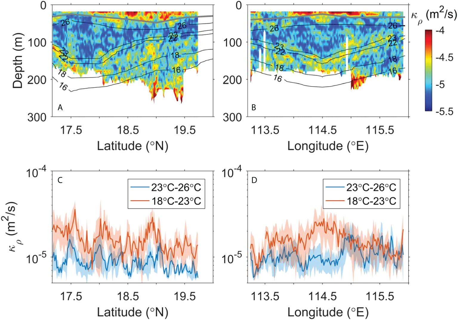
Figure 6 (A, B) are depth profiles of diffusivity κρ on transect S1 and transect S2, respectively. Grey lines indicate the MLD. Isotherms of 26°C, 23°C, 22°C, 18°C, and 16°C are indicated. (C) is the averaged diffusivities between isotherm depths of 23°C and 26°C and between isotherm depths of 18°C and 23°C on transect S1. (D) same as (C) but for transect S2. Shades indicate the corresponding standard deviation of diffusivity.

In summary, the lower boundary of the lens-shaped structure showed significantly elevated diapycnal mixing through shear instability of the eddy‐induced currents (Figures 5, 6). The Richardson number Ri was greatly reduced to ≤¼ due to the significant enhancement of S².

3.4 Origin and development of the ACE

To determine the origin of the studied anticyclonic eddy, historical salinity and temperature data for the Kuroshio Current in the northern SCS (17°–20° N, 114°–117° E) and the Pacific Ocean (19°–22° N, 121°–122.5° E) were obtained from the Argo Data Center and compared to in situ T/S data (Figure 7). Historical profiles of the northern SCS and the Kuroshio Current were derived by averaging 2,443 and 654 data profiles, respectively. A comparison of the water mass characteristics within and outside of the eddy, as well as historical data from the northern SCS and Kuroshio Current, revealed that the upper layer of water within the eddy differed significantly from the upper layer of water outside of the eddy and from the upper layer of water from the northern SCS. This finding indicates that the studied anticyclonic eddy originated from the Kuroshio Current.

FIGURE 7

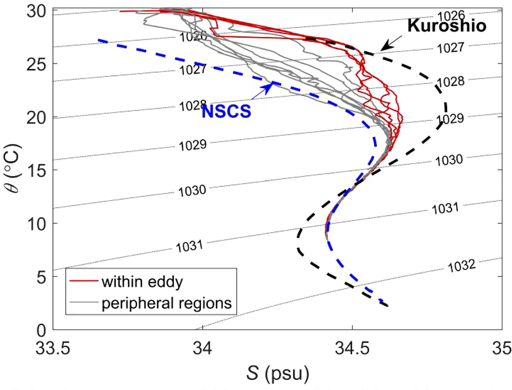
Figure 7 Diagram of θ–S for the water mass within and outside of the eddy examined in this study, in relation to the Kuroshio Current and northern SCS.

The AVISO Mesoscale Eddy Trajectory Atlas product was adopted to confirm the origin of the eddy. These data show that the mesoscale eddy was generated in Luzon Strait on 16 October, 2020, moved to the southwest, and then disappeared at 114°E, 17°N on 27 November, 2021 (Figure 8A). The survival time of this anticyclonic eddy (>12 months) was longer than that of most ocean eddies (Chelton et al., 2011a). The abnormally low SSTs within the eddy (Figure 8C) were present in the early stage of eddy formation in the Luzon Strait. SSTs derived from MODIS during five different periods are shown in Figures 8B–F. According to the 8-day composite SST data collected from 31 November, 2020 to 7 December, 2020, high, rather than low, SSTs were detected in the eddy core (Figure 9B). Lower SSTs appeared within the eddy during the period from 25 January to 1 February, 2021, and continued thereafter (Figures 4, 8C–F). Thus, the ACE persisted existed for a long period between its early formation and extinction.

FIGURE 8

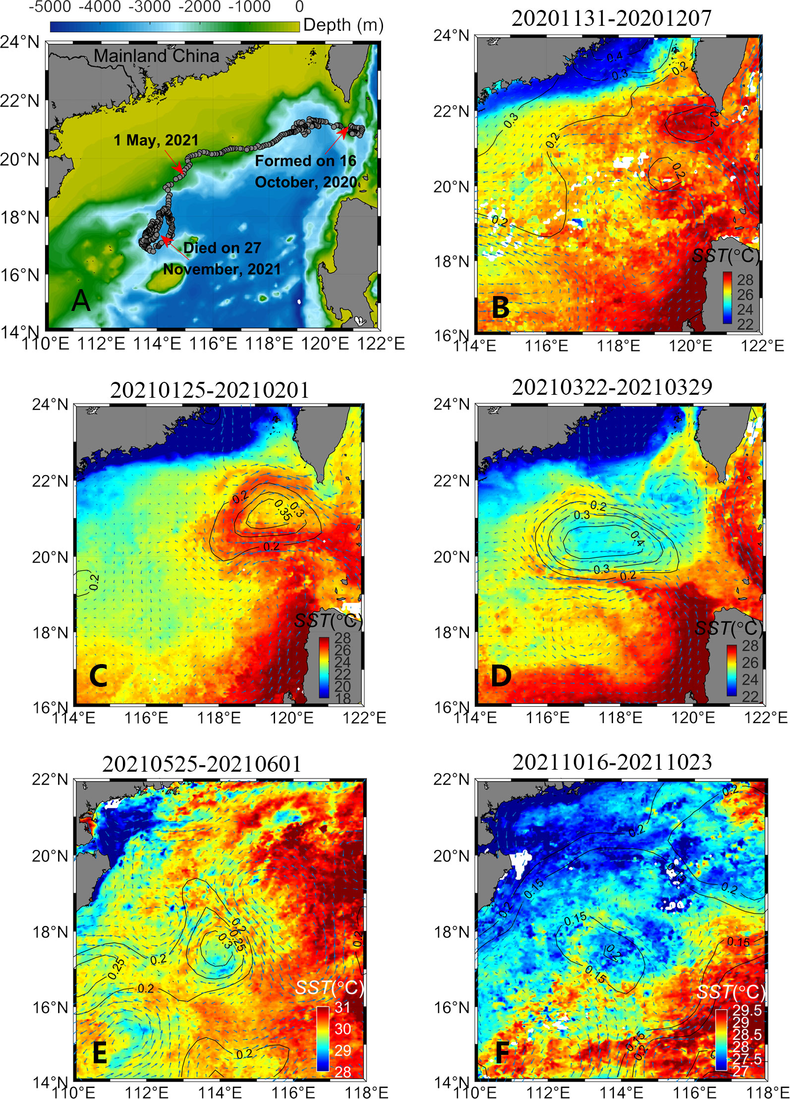
Figure 8 (A) Trajectory of the studied eddy. (b–f) MODIS 8-day composite SSTs in the northeastern SCS for the periods 31 November–7 December 2020, 25 January–1 February 2021, 22–29 March 2021, 25 May–1 June 2021, and 16–23 October 2021. Eddy formation time and location are indicated in (A). Black lines in (B–F) indicate the 0.2, 0.25, 0.3, 0.35, and 0.4 m contours of 8-day averaged SLA. Sea surface geostrophic currents are also indicated.

FIGURE 9

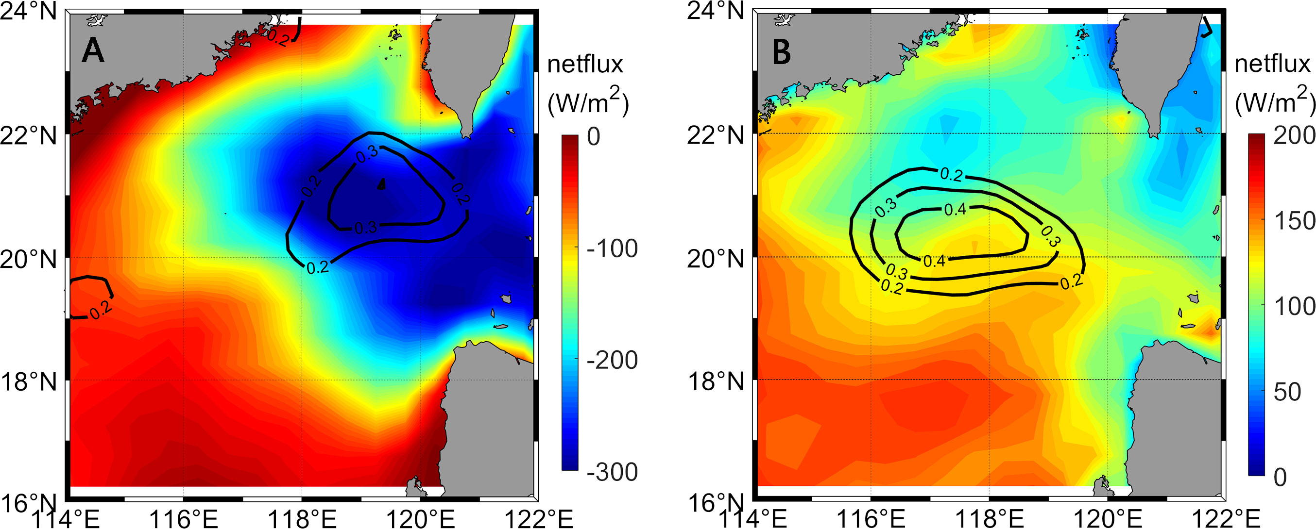
Figure 9 (A) and (B) are the averaged net downwards heat flux at the surface for the periods 25 January–1 February 2021 and 22–29 March 2021. Black lines indicate the SLA.

Previous studies have demonstrated that ACEs with lower SSTs are not uncommon in the northern SCS and northern Pacific Ocean (Sun et al., 2019; Sun et al., 2021). In the northern SCS, many such eddies form in the Luzon Strait. Sun et al. (2021) observed that abnormal eddies appear to have much shorter survival times than normal eddies, sometimes lasting for only 5–10 days. Normal eddies in the SCS have an average lifespan of approximately 50 days (Lin et al., 2015), and similar lifespans have been observed in abnormal eddies of the northern Pacific Ocean (Sun et al., 2019), the abnormal eddy examined in the present study appears to be an unusual case for the SCS.

4 Discussion

4.1 Proposed generation mechanism of the surface cold-core ACE

In the SCS, ACEs mainly appear to the northwest of the Luzon Strait, under the influence of Kuroshio Current intrusions (Sun et al., 2021). The ACE examined in this study also originated from a Kuroshio intrusion (Figure 8). In the early stage of eddy formation, a warm-water Kuroshio intrusion was observed (Figure 8B). Over time, a loop appeared in the path of the Kuroshio Current, and a cold-water mass was trapped in the eddy core (Figure 8C). Subsequently, the water mass was pinched off from the Kuroshio Current to form the eddy, which then migrated into the SCS.

In order to study the mechanism of the surface cold-core ACE, temperature budgets of two periods 25 January-1 February 2021 and 22-29 March 2021 are calculated. The temperature budget equation is was evaluated using the equation given by Huang et al., 2010,

$$T_t=Q_{Hor-Adv}+Q_w+Q_q+Q_{zz}$$

(2)

where T_t is the surface layer temperature tendency, which is a sum of horizontal advection (Q_Hor-Adv), vertical entrainment (Q_w), net surface heat flux (Q_q), and vertical diffusion (Q_zz). Within a short period of 8 days, the eddy remained stable that the shape and size are relatively consistent, thus Q_w and Q_zz are supposed to be ignored. Then the right side of equation (2) remains Q_Hor-Adv and Q_q.

Term of Q_q are derived by the averaged hourly timeseries analysis data of the NCEP Climate Forecast System Version 2 (http://apdrc.soest.hawaii.edu/datadoc/cfsv2_hourly_ts.php), which is calculated as the sum of the net shortwave radiation (NSW), net longwave radiation (NLW), latent heat flux (LHF), and sensible heat flux (SHF). Q_Hor-Adv is a sum of zonal advection and meridional advection,

$$Q_{Hor-Adv}=-\rho C_{p}h\left(u\frac{\partial T}{\partial x}+v\frac{\partial T}{\partial y}\right)$$

(3)

Here ρ is the density of the seawater (1025 kg/m³), C_p is the specific heat capacity of the seawater [3903 J/(Kg·K)], h is set to 20 m as we focus on the near sea surface process.

Figure 9 shows the total downward heat flux at surface for the periods 25 January-1 February 2021 and 22-29 March 2021, respectively. For the period 25 January-1 February 2021, net surface fluxes within the eddy were less than -200 W/m2, indicating the surface of ocean is losing heat rapidly. And for the period 22-29 March 2021, net surface fluxes within eddy changed to positive. Averaged net surface fluxes in the cold-core region of the eddy for those two periods were -256 W/m2 and 99 W/m2, respectively. Here the cold-core area is defined as a closed area with an SLA of 0.3 m (Figures 8C, D).

The horizontal advection is calculated by analysis datasets of the global ocean physics analysis and forecast system (GLOBAL_ANALYSIS_FORECAST_PHY_001_024) distributed by the Copernicus Marine Environment Monitoring Service (CMEMS; http://marine.copernicus.eu/). Firstly, validation of CMEMS analysis is shown. Comparing with the satellite remote sensing data of MODIS (Figures 8C, D), CMEMS analysis is able to reproduce the SST features in the study region (Figures 10A, B). Figures 10C, D show the horizontal advection. A negative (positive) flux indicates the cold (warm) advection. Averaged net surface fluxes in the cold-core region of the eddy for those two periods was -15 W/m2 and -32 W/m2, respectively.

FIGURE 10

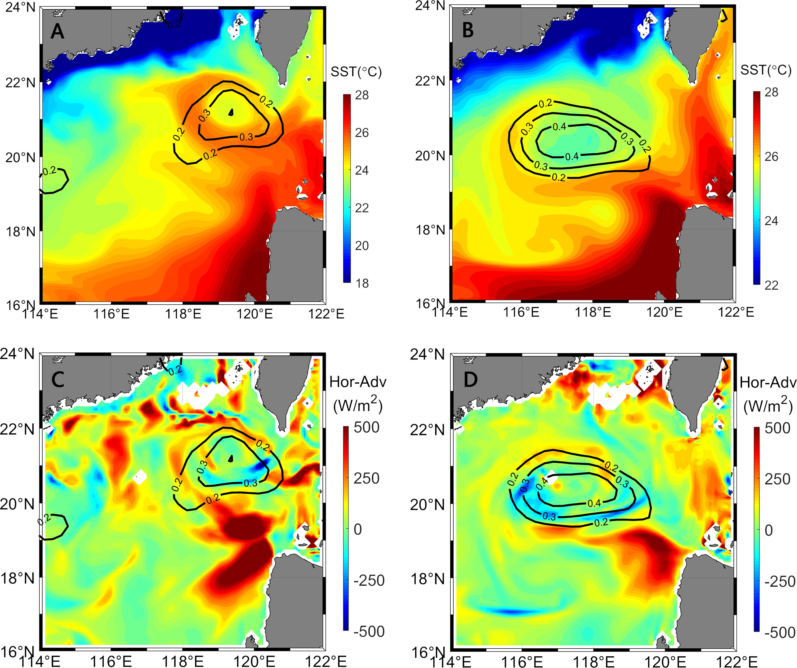
Figure 10 (A) and (B) are the CMEMS analysis 8-day averaged SSTs for the periods 25 January–1 February 2021 and 22–29 March 2021, respectively. (C) and (D) are the averaged horizontal advection for the two periods. Black lines indicate the SLA.

For the period 25 January-1 February 2021, the horizontal advection within the cold-core region was much smaller than the net surface flux, suggesting that formation of the surface cold-core eddy was closely related to air-sea interactions in winter. In the loop of the Kuroshio Current, warm water was supplied by Kuroshio waters at low latitudes, whereas the core of eddy received no warm water supply, but continuous surface cooling, in the winter, decreasing the water temperature at the center relative to that in the Kuroshio loop (Figure 11). With the eddy propagating westward (22-29 March 2021), compared with the net surface flux, the horizontal advection cannot be ignored. The former is positive value of 99 W/m² and the latter is negative value of -32 W/m², meaning the horizontal advection is important to maintain the surface cold-core feature of the ACE as it propagated westward.

FIGURE 11

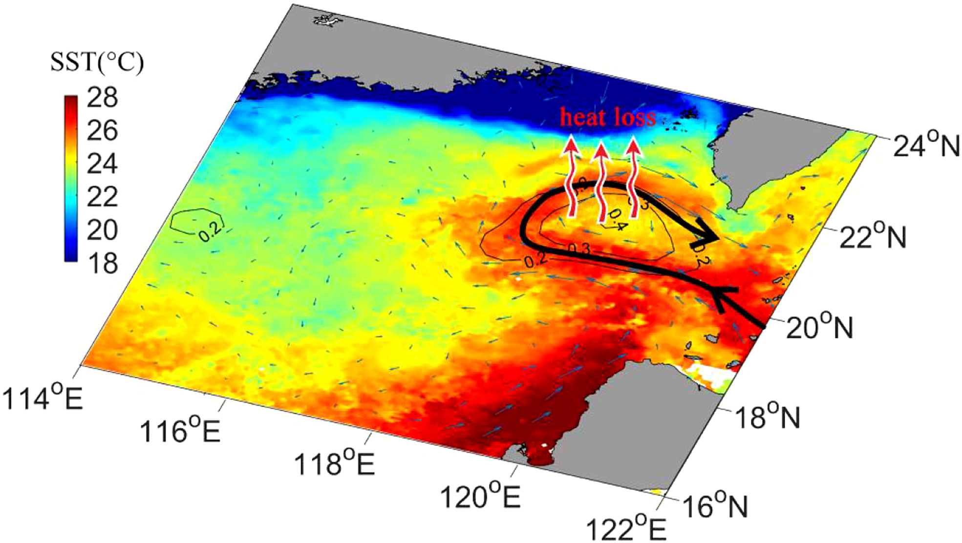
Figure 11 Sketch of the generation of the surface cold-core anticyclonic eddy following heat loss at its core. Background colors indicate MODIS 8-day composite SSTs during 25 January–1 February 2021. Black line indicates a loop in the path of the Kuroshio Current. Red arrow indicates ocean heat loss.

4.2 Possible generation mechanism of the lens-shaped feature of the ACE

The formation of lens-shaped feature in the eddy may be closely related to the vertical distribution of water velocity. The observed data show that a subsurface speed maximum appeared at depth of 90 m in the center of the lens-shaped structure, in the vertical direction (Figures 5A, E). Above (below) that depth, velocity decreased with decreasing (increasing) depth. This subsurface speed maximum induced the lens-shaped structure, as explained through the following thermal wind relationship:

$$\frac{\partial u}{\partial z}=\frac{1}{f{\rho }_0}\frac{\partial \rho }{\partial y}$$

, and

$$\frac{\partial v}{\partial z}=–\frac{1}{f{\rho }_0}\frac{\partial \rho }{\partial x}$$

(2)

where u and v represent the zonal and meridional velocity, respectively, ρ₀ is the reference density (1025 kg/m³), ρ is the potential density of sea water, and f is the local Coriolis parameter. Negative (positive) values of the meridional velocity

∂v/∂z correspond to positive (negative) ∂ρ/∂x values at the left (right) side of the eddy, above the center of the lens-shaped structure, in the vertical direction. Below the center of the structure, in the vertical direction, positive (negative) ∂v/∂z values occur at the left (right) side of the eddy, corresponding to negative (positive) values of ∂ρ/∂x. This subsurface speed maximum resulting from the geostrophic equilibrium relationship is likely the main reason for the formation and maintenance of this lens-shaped structure beneath the surface (Figure 12B).

FIGURE 12

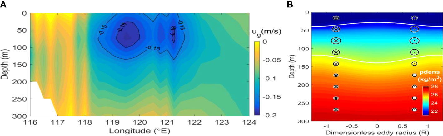
Figure 12 (A) Distribution of geostrophic zonal flow (u_g) along S0 in January, derived from the WOA01 annual mean data set. Negative values indicate westward zonal geostrophic flow. (B) Sketch of the generation of the lens-shaped anticyclonic eddy, caused by the subsurface geostrophic speed maximum. Circled × indicates outward current flow; circled dot indicates inward current flow. The sizes of circled × and dot represent the intensity of the velocity. White line indicates the lens shape of the eddy.

Recently, subsurface speed maxima between 40 and 120 m in the northern SCS were confirmed by mooring observations (Wang et al., 2020); the studied eddy originated from such an intrusion in the Luzon Strait, experienced shoals during this intrusion, and finally disappeared on the western slope of the northern SCS. These subsurface speed maxima in the Luzon Strait are weak in summer and are strong in winter, resulting in a negative correlation with Kuroshio Current strength (Wang et al., 2020). Strong subsurface speed maximum intrusions result in strong baroclinic instability, triggering vigorous baroclinic conversion, leading to active mesoscale eddy variability in the northern SCS, and vice versa.

Zonal geostrophic flow along 21°N in the northern SCS (i.e., transect S0 in Figure 1) reflects the intrusion of the subsurface speed maximum from the entrance of the Luzon Strait to the northern SCS (Figure 12A). The geostrophic flow was calculated from the thermal wind relationship using January climatological temperature and salinity fields obtained from the World Ocean Atlas 2001, selecting 1,000 m as the reference level. The results show a subsurface speed maximum between 50 and 100 m and between 119 and 120°E. Negative values indicate westward flow from the Luzon Strait to the northern SCS. This feature was also confirmed by Wang et al. (2020).

The studied eddy was generated in late October 2020 and persisted until November 2021, indicating a lifespan of >1 year (Figure 8A). It is reasonable to infer that the subsurface speed maximum and lens-shaped structure were present throughout the eddy’s life cycle. The subsurface speed maximum intrusion from the Kuroshio Current appears to have formed the lens-shaped structure of the anticyclonic eddy. This structure maintained the subsurface speed maximum as the eddy migrated west within the SCS, carrying warm saline water; this process may be the main mode of transport of Kuroshio Water to the center and west of the SCS, which maintains a high‐pressure belt along the northern SCS slope and allows material exchange between the continental shelf and open sea (Wang et al., 2010; Wang et al., 2013; Wang et al., 2015).

4.3 Potential impact of the ACE

The SML is the conduit through which the atmosphere influences the ocean interior; conversely, the ocean regulates fluxes into the atmosphere. Mesoscale eddies modulate the spatial and temporal evolution of the mixed layer (Klein et al., 1998; Gaube et al., 2019), and surveys have shown that the MLD is deeper in anticyclonic eddies (Williams, 1988; Waite et al., 2007; Qi et al., 2021). The present study reveals a new type of anticyclonic eddy, with shallower MLD dominated by a lens-shaped structure caused by subsurface speed maximum intrusion from the Kuroshio Current, which is a distinct mechanism from the mixing of local mixed-layer and coastal current water (Lin et al., 2017), salinity-forced restratification of the sea surface (He et al., 2020), and subsurface mode-water forms (McGillicuddy, 2015; Gordon et al., 2017; Zhang et al., 2017). In a normal anticyclonic eddy, deeper MLD and enhanced mixing lead to enhanced nutrient fluxes in regions where the nutricline is collocated with the base of the mixed layer (Gaube et al., 2019). As a consequence, the relationship between anticyclonic or cyclonic eddies and the MLD can form a basis for parameterizing the effects of mesoscale eddies on biogeochemical cycling (Harrison et al., 2018). By contrast, these effects of anticyclonic eddies on biogeochemical cycling would not hold for the abnormal eddy examined in this study. The shallower MLD of the abnormal eddy indicates a weakening of the vertical nutrient flux, reflecting much lower upper-ocean productivity within eddies (Sherin et al., 2018). ACEs in the northern SCS originate from the shedding of Kuroshio water (Figure 9) and are common in the northern SCS (Sun et al., 2021), indicative of their considerable influence on local biogeochemistry.

Anticyclonic eddies are also usually found to have physical impacts, such as increased SSTs, wind speeds, and air–sea heat fluxes (Frenger et al., 2013; Villas Bôas et al., 2015; Byrne et al., 2016). Anticyclonic eddies are associated with positive heat flux anomalies that tend to warm the marine atmospheric boundary layer. However, the ACE examined in this study had low core SSTs. Negative heat flux anomalies probably arise under these conditions. SST images are useful for confirming ocean mesoscale eddies that are tracked and classified based on SST signatures, particularly in the northern SCS (Qiu et al., 2020). Our results may have a profound impact on knowledge of local heat budgets that cannot be captured by coarse-resolution, non-eddy-resolving regional oceanic models.

5 Conclusion

An abnormal anticyclonic eddy characterized by a lens-shaped structure, low SSTs, and shallower MLD was observed in the northern SCS in September 2021. To the best of our knowledge, this is the first study to report such an anticyclonic eddy in the ocean. Normal anticyclonic eddies typically have high SSTs, deeper MLD, and a bowl-shaped structure under the action of geostrophy. The main abnormal feature of the studied eddy is a lens-shaped structure of temperature and density below the SML. A lens of relatively well-mixed water was squeezed between two high-gradient layers that defined the upper and lower bounds of its structure, which was clearly observed at a vertical depth between the 26°C and 22°C isotherms, at approximately 25–150 m. Within the lens-shaped structure, the isothermal layers were stretched, but accompanied by a lower vertical shear of horizontal velocity, higher Richardson number, and a water mixing rate that was one order weaker than that of the surrounding water. A subsurface speed maximum was detected at the center of the lens-shaped structure, in the vertical direction. Another abnormal feature was lower SSTs at core of the anticyclonic eddy, at approximately 30.2°C in the peripheral regions of the eddy, and 0.4°C lower at its core. This cold core was confirmed using MODIS satellite data, demonstrating that anticyclonic eddies are not always equivalent to warm eddies. A third abnormal feature of the studied eddy was the shallower MLD at its center; the MLD was approximately 50 m outside the eddy, and ≈25 m at its center.

The abnormal anticyclonic eddy originated from a Kuroshio Current intrusion in late October 2020, and persisted for >1 year. MODIS data revealed that the cold core was present early in the development of the eddy. Before the eddy was shed from the Kuroshio loop, warm water in the path of the loop was supplied from Kuroshio waters at low latitudes. By contrast, the eddy core received no supplement of warm water, but experienced continuous surface cooling in winter, leading to the development of its cold core. The subsurface speed maximum of the Kuroshio intrusion in the Luzon Strait, also recently confirmed by Wang et al. (2020), appears to be a key mechanism for the generation of this lens-shaped structure, which causes shallower MLD at the center of the anticyclonic eddy.

The phenomenon of anticyclonic eddy formation through water shedding from a Kuroshio loop is common in the northern SCS, indicating that the studied abnormal mesoscale eddy is not unique. Such eddies are expected to have different physical and biogeochemical influences, and potentially to have far-reaching implications for local heat budgets and regional oceanic models. To understand these influences in greater depth, further observational studies are required.

Data availability statement

The raw data supporting the conclusions of this article will be made available by the authors, without undue reservation.

Author contributions

YQ: conceptualization. XL, ZY, KX, HX, YY, WZ, and FZ: data curation. HM and YD: supervision. YQ, HM, and LY: writing—review. All authors contributed to the article and approved the submitted version.

Funding

This study is supported by the National Key R&D Plan of China under contract Nos 2021YFC2803104 and 2021YFC3101301; Key Special Project for Introduced Talents Team of Southern Marine Science and Engineering Guangdong Laboratory (Guangzhou) (GML2019ZD0303); the National Natural Science Foundation of China under contract Nos 42006020 and 41876022; the Guangdong Science and Technology Project under contract No 2019A1515111044. The CAS Key Technology Talent Program under contract No 202012292205.

Acknowledgments

Data and samples were collected onboard of R/V Shiyan 6, we thank the crew for their help during the cruise.

Conflict of interest

The authors declare that the research was conducted in the absence of any commercial or financial relationships that could be construed as a potential conflict of interest.

Publisher’s note

All claims expressed in this article are solely those of the authors and do not necessarily represent those of their affiliated organizations, or those of the publisher, the editors and the reviewers. Any product that may be evaluated in this article, or claim that may be made by its manufacturer, is not guaranteed or endorsed by the publisher.

References

Bryden H. L., Brady E. C. (1989). Eddy momentum and heat fluxes and their effect on the circulation of the equatorial pacific ocean. J. Mar. Res. 47, 55–79. doi: 10.1357/0022240054663187

CrossRef Full Text | Google Scholar

Byrne D., Munnich M., Frenger I., Gruber N. (2016). Mesoscale atmosphere ocean coupling enhances the transfer of wind energy into the ocean. Nat. Commun. 7, 11867. doi: 10.1038/ncomms11867

CrossRef Full Text | Google Scholar

Castellani M. (2006). Identification of eddies from sea surface temperature maps with neural networks. Int. J. Remote Sens. 27, 1601–1618. doi: 10.1080/01431160500462170

CrossRef Full Text | Google Scholar

Chelton D. B., Gaube P., Schlax M. G., Early J. J., Samelsom R. M. (2011b). The influence of nonlinear mesoscale eddies on near-surface oceanic chlorophyll. Science 334, 328–332. doi: 10.1126/science.1208897

PubMed Abstract | CrossRef Full Text | Google Scholar

Chelton D. B., Schlax M. G., Samelson R. M. (2011a). Global observations of nonlinear mesoscale eddies. Prog. Oceanog. 91, 167–216. doi: 10.1016/j.pocean.2011.01.002

CrossRef Full Text | Google Scholar

Chelton D. B., Schlax M. G., Samelson R. M., de Szoeke R. A. (2007). Global observations of large oceanic eddies. Geophys. Res. Lett. 34, L15606. doi: 10.1029/2007GL030812

CrossRef Full Text | Google Scholar

Dillon T. M. (1982). Vertical overturns: A comparison of Thorpe and ozmidov length scales. J. Geophys. Res.- Oceans. 87, 9601–9613. doi: 10.1029/JC087iC12p09601

CrossRef Full Text | Google Scholar

Dong C. M., McWilliams J. C., Liu Y., Chen D. K. (2014). Global heat and salt transports by eddy movement. Nat. Commun. 5, 3294. doi: 10.1038/ncomms4294

PubMed Abstract | CrossRef Full Text | Google Scholar

Dong C. M., Nencioli F., Liu Y., Williams J. C. (2011). An automated approach to detect oceanic eddies from satellite remotely sensed sea surface temperature data. IEEE Geosci. Remote S. 8, 1055–1059. doi: 10.1109/LGRS.2011.2155029

CrossRef Full Text | Google Scholar

Evans D. G., Frajka-Williams E., Naveira, Garabato A. C. (2022). Dissipation of mesoscale eddies at a western boundary via a direct energy cascade. Sci. Rep-UK. 12, 887. doi: 10.1038/s41598-022-05002-7

CrossRef Full Text | Google Scholar

Everett J. D., Baird M. E., Oke P. R., Suthers I. M. (2012). An avenue of eddies: Quantifying the biophysical properties of mesoscale eddies in the Tasman Sea. Geophys. Res. Lett. 39, L16608. doi: 10.1029/2012GL053091

CrossRef Full Text | Google Scholar

Faghmous J. H., Frenger I., Yao Y. S., Warmka R., Lindell A., Kumar V. (2015). A daily global mesoscale ocean eddy dataset from satellite altimetry. Sci. Data. 2, 150028. doi: 10.1038/sdata.2015.28

PubMed Abstract | CrossRef Full Text | Google Scholar

Ferrari R., Wunsch C. (2009). Ocean circulation kinetic energy: Reservoirs, sources, and sinks. Annu. Rev. Fluid Mech. 41, 253–282. doi: 10.1146/annurev.fluid.40.111406.102139

CrossRef Full Text | Google Scholar

Frenger I., Gruber N., Knutti R., Munnich M. (2013). Imprint of southern ocean eddies on winds, clouds and rainfall. Nat. Geosci. 6, 608–612. doi: 10.1038/ngeo1863

CrossRef Full Text | Google Scholar

Frenger I., Münnich M., Gruber N., Knutti R. (2015). Southern ocean eddy phenomenology. J. Geophys. Res.- Oceans. 120, 7413–7449. doi: 10.1002/2015JC011047

CrossRef Full Text | Google Scholar

Gaube P., McGillicuddy D. J., Chelton D. B., Behrenfeld M. J., Strutton P. G. (2014). Regional variations in the influence of mesoscale eddies on near-surface chlorophyll. J. Geophys. Res.-Oceans. 119, 8195–8220. doi: 10.1002/2014JC010111

CrossRef Full Text | Google Scholar

Gaube P., McGillicuddy D. J., Moulin A. J. (2019). Mesoscale eddies modulate mixed layer depth globally. Geophys. Res. Lett. 46, 1505–1512. doi: 10.1029/2018GL080006

CrossRef Full Text | Google Scholar

Gordon A. L., Shroyer E., Murty V. S. (2017). An intrathermocline eddy and a tropical cyclone in the bay of Bengal. Sci. Rep-UK. 7, 46218. doi: 10.1038/srep46218

CrossRef Full Text | Google Scholar

Harrison C. S., Long M. C., Lovenduski N. S., Moore J. K. (2018). Mesoscale effects on carbon export: A global perspective. Global Biogeochem. Cy. 32, 680–703. doi: 10.1002/2017GB005751

CrossRef Full Text | Google Scholar

Hausmann U., McGillicuddy D. J., Marshall J. (2017). Observed mesoscale eddy signatures in southern ocean surface mixed-layer depth. J. Geophys. Res.- Oceans. 122, 617–635. doi: 10.1002/2016JC012225

CrossRef Full Text | Google Scholar

He Q. Y., Zhan H. G., Cai S. Q. (2020). Anticyclonic eddies enhance the winter barrier layer and surface cooling in the bay of Bengal. J. Geophys. Res.-Oceans. 125, e2020JC016524. doi: 10.10292020/JC016524

CrossRef Full Text | Google Scholar

Huang B., Xue Y., Zhang D., Kumar A., McPhaden M. J. (2010). The NCEP GODAS ocean analysis of the tropical pacific mixed layer heat budget on seasonal to interannual time scales. J. Clim. 23, 4901–4925. doi: 10.1175/2010JCLI3373.1

CrossRef Full Text | Google Scholar

Isern-Fontanet J., Chapron B., Lapeyre G., Klein P. (2006). Potential use of microwave sea surface temperatures for the estimation of ocean currents. Geophys. Res. Lett. 33, L24608. doi: 10.1029/2006gl027801

CrossRef Full Text | Google Scholar

Itoh S., Yasuda I. (2010). Water mass structure of warm and cold anticyclonic eddies in the western boundary region of the subarctic North Pacific. J. Phys. Oceanogr. 40, 2624–2642. doi: 10.1175/2010JPO4475

CrossRef Full Text | Google Scholar

Kadko D., Pickart R. S., Mathis J. (2008). Age characteristics of a shelfbreak eddy in the western Arctic and implications for shelfbasin exchange. J. Geophys. Res.-Oceans. 113, C02018. doi: 10.1029/2007jc004429

CrossRef Full Text | Google Scholar

Klein P., Treguier A.-M., Hua B. L. (1998). Three-dimensional stirring of thermohaline fronts. J. Mar. Res. 56, 589–612. doi: 10.1357/002224098765213595

CrossRef Full Text | Google Scholar

Leyba I. M., Saraceno M., Solman S. A. (2017). Air-sea heat fluxes associated to mesoscale eddies in the southwestern Atlantic Ocean and their dependence on different regional conditions. Clim. Dynam. 49, 2491–2501. doi: 10.1007/s00382-016-3460-5

CrossRef Full Text | Google Scholar

Liang C. R., Chen G. Y., Shang X. D. (2017). Observations of the turbulent kinetic energy dissipation rate in the upper central South China Sea. Ocean Dynam. 67, 597–609. doi: 10.1007/s10236-017-1051-6

CrossRef Full Text | Google Scholar

Lin X. Y., Dong C. M., Chen D. K., Liu Y., Yang J. S., Zou B., et al. (2015). Three-dimensional properties of mesoscale eddies in the South China Sea based on eddy-resolving model output. Deep-Sea Res. Pt I. 99, 46–64. doi: 10.1016/j.dsr.2015.01.007

CrossRef Full Text | Google Scholar

Lin H. Y., Hu J. Y., Liu Z. Y., Belkin I. M., Sun Z. Y., Zhu J. (2017). A peculiar lens-shaped structure observed in the South China Sea. Sci. Rep. -UK. 7, 478. doi: 10.1038/s41598-017-00593-y

CrossRef Full Text | Google Scholar

Liu Y. L., Yu L. S., Chen G. (2020). Characterization of sea surface temperature and air-sea heat flux anomalies associated with mesoscale eddies in the south China Sea. J. Geophys. Res.-Oceans. 125, e2019JC015470. doi: 10.1029/2019JC015470

CrossRef Full Text | Google Scholar

Liu Y. L., Zheng Q. A., Li X. F. (2021). Characteristics of global ocean abnormal mesoscale eddies derived from the fusion of sea surface height and temperature data by deep learning. Geophys. Res. Let. 48, e2021GL094772. doi: 10.1029/2021GL094772

CrossRef Full Text | Google Scholar

Martin A. P., Richards K. J. (2001). Mechanisms for vertical nutrient transport within a north Atlantic mesoscale eddy. Deep-Sea Res. Pt II. 48, 757–773. doi: 10.1016/S0967-0645(00)00096-5

CrossRef Full Text | Google Scholar

Mathis J. T., Pickart R. S., Hansell D. A., Kadko D., Bates N. R. (2007). Eddy transport of organic carbon and nutrients from the chukchi shelf: Impact on the upper halocline of the western Arctic Ocean. J. Geophys. Res.-Oceans. 112, C05011. doi: 10.1029/2006JC003899

CrossRef Full Text | Google Scholar

McCoy D., Bianchi D., Stewart A. L. (2020). Global observations of submesoscale coherent vortices in the ocean. Prog. Oceanogr. 189, 102452. doi: 10.1016/j.pocean.2020.102452

CrossRef Full Text | Google Scholar

McGillicuddy D. J. (2015). Formation of intrathermocline lenses by eddy–wind interaction. J. Phys. Oceanogr. 45, 606–612. doi: 10.1175/JPO-D-14-0221.1

CrossRef Full Text | Google Scholar

McGillicuddy D. J., Anderson L. A., Bates N. R., Bibby T., Buesseler K. O., Carlson C. A., et al. (2007). Eddy/wind interactions stimulate extraordinary mid-ocean plankton blooms. Science 316, 1021–1026. doi: 10.1126/science.1136256

PubMed Abstract | CrossRef Full Text | Google Scholar

Pickart R. S., Weingartner T. J., Pratt L. J., Zimmermann S., Torres D. J. (2005). Flow of winter transformed pacific water into the Western Arctic. Deep-Sea Res. Pt II. 52, 3175–3198. doi: 10.1016/j.dsr2.2005.10.009

CrossRef Full Text | Google Scholar

Qi Y. F., Mao H. B., Wang X., Yu L. H., Lian S. M., Li X. P., et al. (2021). Suppressed thermocline mixing in the center of anticyclonic eddy in the north South China Sea. J. Mar. Sci. Eng. 9, 1149. doi: 10.3390/jmse9101149

CrossRef Full Text | Google Scholar

Qi Y. F., Shang C., Mao H., Qiu C. H., Liang C. R., Yu L. H., et al. (2020). Spatial structure of turbulent mixing of an anticyclonic mesoscale eddy in the northern South China Sea. Acta Oceanol. Sin. 39, 69–81. doi: 10.1007/s13131-020-1676-z

CrossRef Full Text | Google Scholar

Qiu C. H., Ouyang J., Yu J. C., Mao H. B., Qi Y. F., Wu J. X., et al. (2020). Variations of mesoscale eddy SST fronts based on an automatic detection method in the northern South China Sea. Acta Oceanol. Sin. 39, 82–90. doi: 10.1007/s13131-020-1669-y

CrossRef Full Text | Google Scholar

Qiu C. H., Liang H., Sun X. J., Mao H. B., Wang D. X., Yi Z. H., et al. (2021). Extreme sea-surface cooling induced by eddy heat advection during tropical cyclone in the northwestern Pacific Ocean. Front. Mar. Sc. 8:726306. doi: 10.3389/fmars.2021.726306

CrossRef Full Text | Google Scholar

Qiu C. H., Yi Z. H., Su D. Y., Wu Z. W., Liu H. L., Lin P. F., et al. (2022). Cross-slope heat and salt transport induced by slope intrusion eddy’s horizontal asymmetry in the northern South China Sea. J. Geophys. Res.-Oceans. 08. doi: 10.1029/2022JC018406

CrossRef Full Text | Google Scholar

Rabinovich A. B., Thomson R. E., Bograd S. J. (2002). Drifter observations of anticyclonic eddies near bussol’ strait, the kuril islands. J. Oceanogr. 58, 661–671. doi: 10.1023/A:1022890222516

CrossRef Full Text | Google Scholar

Sherin C. K., Sarma V. V. S. S., Rao G. D., Viswanadham R., Omand M. M., Murty V. S. N. (2018). New to total primary production ratio (f-ratio) in the bay of Bengal using isotopic composition of suspended particulate organic carbon and nitrogen. Deep-Sea Res. Pt I. 139, 43–54. doi: 10.1016/j.dsr.2018.06.002

CrossRef Full Text | Google Scholar

Shimizu Y., Yasuda I., Ito S. (2001). Distribution and circulation of the coastal oyashio intrusion. J. Phys. Oceanogr. 31, 1561–1578. doi: 10.1175/1520-0485(2001)031<1561:dacotc>2.0.co;2

CrossRef Full Text | Google Scholar

Spall M. A., Pickart R. S., Fratantoni P. S., Plueddemann A. J. (2008). Western Arctic Shelfbreak eddies: Formation and transport. J. Phys. Oceanogr. 38, 1644–1668. doi: 10.1175/2007JPO3829.1

CrossRef Full Text | Google Scholar

Sun W. J., Dong C. M., Tan W., He Y. J. (2019). Statistical characteristics of cyclonic warm-core eddies and anticyclonic coldcore eddies in the north pacific based on remote sensing data. Remote Sens.-Basel. 11, 208. doi: 10.3390/rs11020208

CrossRef Full Text | Google Scholar

Sun W. J., Liu Y., Chen G. X., Tan W., Lin X. Y., Guan Y. P., et al. (2021). Three-dimensional properties of mesoscale cyclonic warm-core and anticyclonic cold-core eddies in the South China Sea. Acta Oceanol. Sin. 40, 17–29. doi: 10.1007/s13131-021-1770-x

CrossRef Full Text | Google Scholar

Thorpe S. A. (2005). The turbulent ocean (Cambridge, UK: Cambridge University Press), 485.

Google Scholar

Timmermans M. L., Toole J., Proshutinsky A., Krishfield R., Plueddemann A. (2008). Eddies in the Canada basin, Arctic ocean, observed from ice-tethered profilers. J. Phys. Oceanogr. 38, 133–145. doi: 10.1175/2007JPO3782.1

CrossRef Full Text | Google Scholar

Villas Bôas A. B., Sato O. T., Chaigneau A., Castelao G. P. (2015). The signature of mesoscale eddies on the air-sea turbulent heat fluxes in the south Atlantic Ocean. Geophys. Res. Lett. 42, 1856–1862. doi: 10.1002/2015GL063105

CrossRef Full Text | Google Scholar

Waite A. M., Pesant S., Griffin D. A., Thompson P. A., Holl C. M. (2007). Oceanography, primary production and dissolved inorganic nitrogen uptake in two leeuwin current eddies. Deep-Sea Res. Pt II. 54, 981–1002. doi: 10.1016/j.dsr2.2007.03.001

CrossRef Full Text | Google Scholar

Wang D. X., Hong B., Gan J. P., Xu H. Z. (2010). Numerical investigation on propulsion of the counter-wind current in the northern South China Sea in winter. Deep-Sea Res. Pt I. 57, 1206–1221. doi: 10.1016/j.dsr.2102.06.07

CrossRef Full Text | Google Scholar

Wang D. X., Wang Q., Zhou W. D., Cai S. Q., Li L., Hong B. (2013). An analysis of the current deflection around dongsha islands in the northern South China Sea. J. Geophys. Res.-Oceans. 118, 490–501. doi: 10.1029/2012JC008429

CrossRef Full Text | Google Scholar

Wang Q., Wang Y. X., Zhou W. D., Wang D. X., Sui D. D., Chen J. (2015). Dynamic of the upper cross isobath’s flow on the north South China Sea in summer. Aquat. Ecosyst. Health 18, 357–366. doi: 10.1080/14634988.2015.1112124

CrossRef Full Text | Google Scholar

Wang Q., Zeng L., Chen J., He Y. K., Zhou W. D., Wang D. X. (2020). The linkage of kuroshio intrusion and mesoscale eddy variability in the northern South China Sea: Subsurface speed maximum. Geophys. Res. Lett. 46, e2020GL087034. doi: 10.1029/2020GL087034

CrossRef Full Text | Google Scholar

Wang Y. T., Zhang H. R., Chai F., Yuan Y. P. (2018). Impact of mesoscale eddies on chlorophyll variability off the coast of Chile. PloS One 13, e0203598. doi: 10.1371/journal.pone.0203598

PubMed Abstract | CrossRef Full Text | Google Scholar

Williams R. (1988). Modification of ocean eddies by air-sea interaction. J. Geophys. Res. 93, 15,523–15,533. doi: 10.1029/JC093iC12p15523

CrossRef Full Text | Google Scholar

Xiu P., Chai F., Shi L., Xue H. J., Chao Y. (2010). A census of eddy activities in the South China Sea during 1993–2007. J. Geophys. Res.-Oceans. 115, C03012. doi: 10.1029/2009JC005657

CrossRef Full Text | Google Scholar

Xu G. J., Dong C. M., Liu Y., Gaube P., Yang J. S. (2019). Chlorophyll rings around ocean eddies in the north pacific. Sci. Rep.-UK. 9, 2056. doi: 10.1038/s41598-018-38457-8

CrossRef Full Text | Google Scholar

Yang X., Xu G. J., Liu Y., Sun W. J., Xiao C. S., Dong C. M. (2020). Multi-source data analysis of mesoscale eddies and their effects on surface chlorophyll in the bay of Bengal. Remote Sens.-Basel. 12, 3485. doi: 10.3390/rs12213485

CrossRef Full Text | Google Scholar

Zhang H. M., Bates J. J., Reynolds R. W. (2006). Assessment of composite global sampling: Sea surface wind speed. Geophys. Res. Lett. 33, L17714. doi: 10.1029/2006GL027086

CrossRef Full Text | Google Scholar

Zhang Z. G., Qiu B. (2020). Surface chlorophyll enhancement in mesoscale eddies by submesoscale spiral bands. Geophys. Res. Lett. 47, e2020GL088820. doi: 10.1029/2020GL088820

CrossRef Full Text | Google Scholar

Zhang Z. G., Wang W., Qiu B. (2014). Oceanic mass transport by mesoscale eddies. Science 345, 322–324. doi: 10.1126/science.1252418

PubMed Abstract | CrossRef Full Text | Google Scholar

Zhang Z. G., Zhang Y., Wang W. (2017). Three-compartment structure of subsurface-intensified mesoscale eddies in the ocean. J. Geophys. Res.-Oceans. 122, 1653–1664. doi: 10.1002/2016JC012376

CrossRef Full Text | Google Scholar