 Wei Zhong
 Jun Lin1,2*
94% of researchers rate our articles as excellent or good
Learn more about the work of our research integrity team to safeguard the quality of each article we publish.
Find out more
ORIGINAL RESEARCH article
Front. Mar. Sci., 23 August 2022
Sec. Physical Oceanography
Volume 9 - 2022 | https://doi.org/10.3389/fmars.2022.973155
This article is part of the Research TopicMulti-Scale Fluid Physics in Oceanic Flows: New Insights from Laboratory Experiments and Numerical SimulationsView all 16 articles
The hydrodynamic effects of the largest suspended mussel farms in the East China Sea near Gouqi Island, was investigated using a high-resolution 3D ocean model and field observations. To capture the 3D farm effects on hydrodynamics, an additional depth dependent momentum sink term was introduced in the model. The model results compared well with the field observations. The present model and observational results indicate that the presence of farms reduces the flow by more than 79%, 55%, and 34% in the upper, middle, and bottom layers at the farm center, respectively. According to the harmonic analysis of predicted current, mussel farms reduce the magnitude of the semidiurnal tidal current and also alter the magnitude and direction of the diurnal tidal current. The blockage by the farm weakens the Eulerian residual tidal current within the farm in the NE-SW direction, while strengthens that at the edge of the farm in the SE-NW direction. Cross sections, Sec1 and Sec2 are perpendicular to these two major residual currents and intercept with the center of the farm from SE to NW and from NE to SW respectively. The farm effect on the total water flux over a month through the Sec2 displays a semi-lunar periodic oscillation and is one order of magnitude smaller than that at Sec1. An asymmetry tidal current was observed in the farm north of Gouqi Island. The field observation of vertical profiles of current suggests that the thickness of surface canopy boundary layer can reach 5 m upstream from the farm during flood tide, increases gradually downstream up to 10 m under the cumulative influences of the farm. And a wake zone was observed downstream from the farm during flood tide. Better understanding of farm-induced hydrodynamic effects provides insight into how to optimize farm layouts based on local hydrodynamics, to maximize farm productivity and minimize environmental impacts.
Global aquaculture production has grown dramatically over the past 50 years to meet the rising demand for food (Mustafa et al., 2017; Garlock et al., 2019). The global shellfish production attained 17.5 million tons in live weight with a value of USD 29.2 billion in 2018, accounting for 56.2% of the total aquaculture production. As the largest producer of aquaculture bivalves in the world, China produced 14.4 million tons, which is 82% of worldwide shellfish production (FAO, 2020). Gouqi Island is located in the East China Sea, just south-east of Shanghai and east of Hangzhou. As one of the top mussel producer in China, the island features a 12 km2 mussel farm with an annual production of more than 180, 000 tons.
The ‘off-bottom’ cultivation with raft, pole, and longline is commonly used for mussel aquaculture to prevent predation by predators such as crabs and starfish. The longline aquaculture system employed in the mussel farms of Gouqi Island, is the most used technology since it requires the least amount of infrastructure (Mascorda Cabre et al., 2021). This farming system forms a suspended canopy and acts as a porous medium in the water column. Suspended canopy such as aquaculture farms on hydrodynamics has received much less attention than submerged or emergent canopy (Plew, 2011a; O’Donncha et al., 2015). Nevertheless, the hydrodynamic effects of suspended canopy is of fundamental importance (Grant and Bacher, 2001; Plew et al., 2005; Stevens et al., 2008; Delaux et al., 2011; O’Donncha et al., 2013, O’Donncha et al., 2015; Duarte et al., 2014; Aguiar et al., 2015; Filgueira et al., 2015; Konstantinou et al., 2015; Lin et al., 2016; Filgueira, 2018; Liu and Huguenard, 2020).
At Gouqi Island, there has been increased in conflicts over coastal space in recent years, as the space suitable for aquaculture has been gradually used up. Accordingly, the fishermen repeatedly lengthen the mussel ropes and raise the stocking density, which causes overstocking. The production and quality of mussels, however, have not increased with the expansion of the aquaculture unit. In addition, the complex flow patterns near the island have led to significant geographical variation in the yield of mussel farms. Therefore, the mussel farms on Gouqi Island needs a comprehensive farming plan to optimize the farming layout and enhance overall productivity and quality.
The hydrodynamics modifications by the aquaculture structures has significant effect on the growth of cultured populations especially non-feeding mussels. The suspended canopy layer inhibits the surface layer water flow, therefore, change the circulation pattern inside and around the farm (Konstantinou et al., 2015; Lin et al., 2016; Konstantinou and Kombiadou, 2020; Liu and Huguenard, 2020). The flow responses to the presence of farm in turn affect the mussel food availability through increased water residence time and nutrient depletion, therefore, the carrying capacity of ecosystem (Byron et al., 2011a; Byron et al., 2011b; Anaïs et al., 2020; Gao et al., 2020). Quantifications of effect of suspended farms on circulation is critical in evaluating carrying capacity, ecosystem sustainable and effective management of the aquaculture activities (Filgueira et al., 2015; Froján et al., 2018; Konstantinou and Kombiadou, 2020).
The objective of this study is to investigate the hydrodynamic effects of a large-scale suspended mussel farms using, in-situ and navigational field observations and 3D ocean circulation numerical model that incorporate the farm effect. Ocean models have become a popular tool to assess the environmental effects and interactions among open water aquaculture systems (Reid et al., 2018; Broch et al., 2020). Thus, a high-resolution three-dimensional hydrodynamic model, Estuarine Coastal Ocean Model semi-implicit (ECOM-si) (Wu and Zhu, 2010; Wu et al., 2011) of Gouqi Island is also developed to further explore the hydrodynamic processes related to farms. To incorporate the blockage effect of the suspended farms into the model, a depth dependent momentum sink term representing the loss of momentum is added to the momentum equations of the model (Roc et al., 2013; Yang et al., 2013; Li et al., 2017; O’Hara Murray and Gallego, 2017). Introduction to the geographic location and farm configurations of Gouqi Island, field observations and numerical model are presented in section 2. In section 3, the field observations, are analyzed to provide insight into the hydrodynamic effects of the farm. In section 4, the model results are compared against the field observations to evaluate the model performance. In section 5, the model results of farm effects on tides are highlighted and discussed. Implications of the present study and future research needs are summarized in section 6.
Gouqi Island is known as the hometown of mussels in China. It has the largest mussel farming area in the East China Sea, with an aquaculture area of 12 km2. It has a subtropical climate, with an average surface water temperature ranges between 17 and 19°C. It is dominated by a semidiurnal tide with a spring tidal range of approximately 2.5 m and neap tidal range of 1.0 m. The western part of the farm is influenced by the runoff of the Changjiang and Qiantang rivers (Figure 1A), while the eastern part of the farm is affected by the Taiwan warm current and Zhebei upwelling, which leads to a large horizontal salinity gradient from the east to the west of the farm (Zhang et al., 2008). A significant amount of nutrients is transported in the aquaculture area by river runoff and strong tidal current, which raises the primary productivity and supplies the farm with a rich food source. Typhoons frequently pass by Gouqi Island and pose a serious threat to the aquaculture infrastructure and personnel. In order to minimize the typhoon damages to the aquaculture facilities, most mussel farms are located to the northwest of Gouqi Island (Figure 1B) which protect the farms from most typhoons come from the southeast. Additionally, a suitable water depth of ~ 20 m and a reasonably close operational distance is convenient for fishermen.
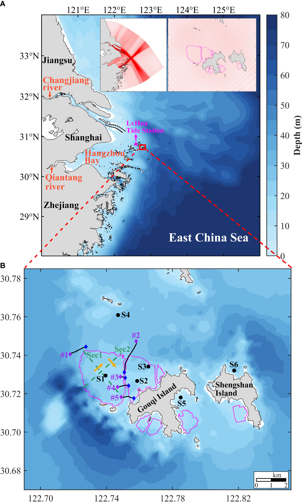
Figure 1 Map of the study area, field stations and model grid system. (A) Geographic location of Gouqi Island. The model domain and mesh. Pink triangle indicates the location of LvHua Tide Station (30°49′N,122°36′E). Red rectangle indicates the range of Gouqi Island area. (B) Field observation stations (S1 to S6). The orange arrows show the positive direction of water transport across Sec1 and Sec2 indicated in green dashed lines. The black lines indicate the boat cruise route #1 to #5 for ADCP measurements. The purple and blue diamond are the starting and end point, respectively. The pink lines indicate the borderlines of suspended mussel farms.
There are seven mussel farming zones in Gouqi Island area (Figure 1B). The largest one is to the northwest of the island with 6.76 km2 (Figure 2A). A suspended aquaculture system is used for mussel farms. The suspended aquaculture system consists of buoys, lanyards, suspended sleeves (aquaculture lines with mussels attached), and longlines used to attach sleeves in the vertical direction (Figure 2C) (Lin et al., 2016). The mussel farms in Gouqi Island are owned by different individuals, which complicate the layouts both within and across the aquaculture units. And it is difficult to count the actual number of mussel sleeves during the field observations.
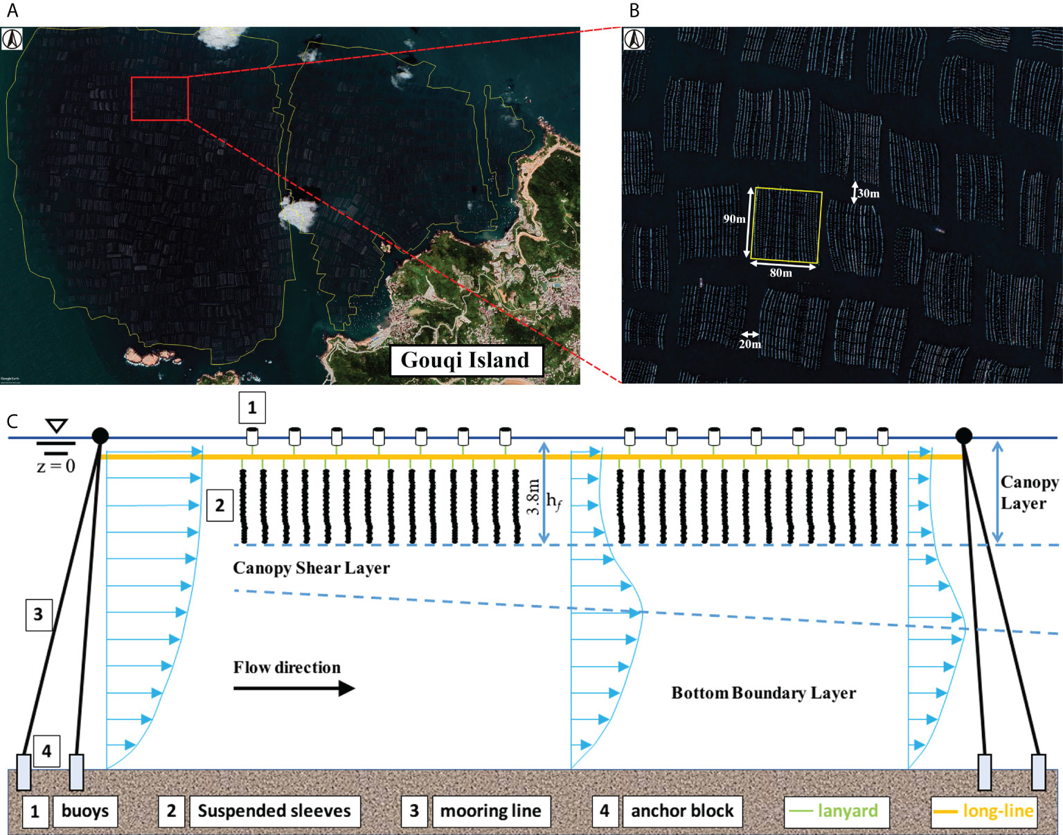
Figure 2 (A) Satellite view of farms at the north of Gouqi Island from Google Earth, August 20, 2018. (B) A zoom-in satellite view of a local farming region that shows the configuration of mussel farms. A typical aquaculture unit of mussel farms outlined by the yellow line. (C) Side view of the components of aquaculture facilities. Three layer flow structures exist around the facility. hf is the farm penetration depth.
Making use of the Google Earth high-resolution remote-sensing image, we estimated that a typical aquaculture unit is roughly 7200 m2 (90m×80m) (Figure 2B), with 20 rows and 90 mussel sleeves in each row. We assumed that the mussel sleeves are evenly distributed across the model grid. Therefore, in the model, the mussel sleeves density is approximately 4 m2 sleeves-1.
In order to investigate the hydrodynamic effects due to mussel farms in Gouqi Island area, in-situ observations of velocity fields and tidal elevations were conducted during spring and neap tidal conditions. An Acoustic Doppler Current Profiler (ADCP) was installed on buoys at the field station S1, S2, S3 and S4 (Figure 1B). Current profiles were measured with a 0.5 m vertical bin using a 500 Hz Teledyne RD Instrument (RDI). The measurements were conducted at S1 for 96 hours starting on July 21, 2020 (spring tide), at S2 for 72 hours starting on July 25, 2020 (neap tide), at S3 for 48 hours starting on March 10, 2021 (spring tide), and at S4 for 25 hours starting on November 5, 2018 (spring tide).
Furthermore, five boat cruise observations were also conducted across mussel farms using a navigational ADCP (Nortek, 1000Hz) mounted on a boat with a 0.2 m vertical bin. The #1 boat cruise track lies in the northwest of Gouqi Island (Figure 1B), from southwest to northeast and away from the farm, nearly paralleling to the coast of the island. The ADCP data was collected for about 7 minutes on July 10, 2021 during spring tide. The #2 boat cruise track is located in the north of Gouqi Island (Figure 1B), stretching from outside to inside of the farm. The ADCP data was collected for about 17 minutes on June 29, 2021 during neap tide. The #3, #4 and #5 boat cruise is located across the waterway between the two major farms (Figure 1B). The ADCP data was collected for about 2, 4 and 5 minutes respectively on July 10, 2021 during spring tide.
The tidal elevation data were collected every 5 minutes at S4, S5 and S6 stations in Figure 1B using a RBR wave tidal gauge. At S4, the tidal data was collected from November 5, 2018 to November 10, 2018. At S5, the tidal data was collected from July 19, 2020 to July 29, 2020. And at S6, the tidal data was collected from November 9, 2018 to November 11, 2018. Also, the tide elevation data at Lvhua tidal station (30°49′N, 122°36′E) from the National Marine Information Center (https://www.cnss.com.cn/tide) was also used to verify the present model results of tidal elevation from July 18, 2020 to July 31, 2020.
In this study, an Estuarine Coastal Ocean Model semi-implicit (ECOM-si) developed by Blumberg (1994) and improved by Wu and Zhu (2010) was used to simulate the hydrodynamic conditions of mussel farms around Gouqi Island. The model uses an orthogonal curvilinear coordinate system that accommodates complicated coastlines. Wu and Zhu (2010) developed a robust third-order advection scheme to reduce the numerical oscillations in solving the transport equations. To increase the computational efficiency, the time step was set to vary automatically based on the Courant-Friedrich-Levy (CFL) criterion (Wu et al., 2011).
In order to quantify the mussel farms blockage effect in the transport equations, the water flux at a given transect is calculated by applying the following equation (Wu et al., 2006; Lin et al., 2015):
where WR(t)|Γ is the water volume flux, with a unit of cubic meters per second, perpendicular to a given transect Γ.
The direction of positive water transport is defined in Figure 1B, d is the local still water depth, ζ is the surface water level, L is the length of the transect Γ, dξ is the line segment along the transect Γ, Vn(x,y,z,t) is the horizontal velocity component perpendicular to the transect Γ
The accumulated total water flux over a time period is calculated by integrating (1) (Zhang et al., 2022):
where τ⋲[t0,tf] is the time interval, t0 the initial time, and tf the final time.
The model domain included the Changjiang River Estuary, the Hangzhou Bay, and part of the East China Sea (Figure 1A). A curvilinear orthogonal coordinate was employed in the horizontal direction, and the sigma coordinate was used in the vertical direction. The horizontal mesh grid was refined to 336×256 cells with the highest spatial resolution of 100 m inside the mussel farms. The model was divided into 35 layers in the vertical direction with refinement in the aquaculture surface layer and the bottom layer. At the offshore open boundary, the model was driven by 16 tidal constituents (M2, S2, N2, K2, K1, O1, P1, Q1, MU2, NU2, T2, L2, 2N2, J1, M1 and OO1), with amplitude and phase from the TPXO7.1 dataset (http://g.hyyb.org/archive/Tide/TPXO/TPXO_WEB/global.html). The annual average discharge of the Changjiang River was set to 30000 m3s-1. A variable time step was taken according to the instantaneous CFL criteria at each time step, with the maximum time step of 30s and the minimum time step of 10s. Only tidal currents were considered in the present study. Wind driven currents and the effects of density stratification (baroclinic force) on circulation were not considered.
In this study, two numerical model cases were carried out. For case 1, the blocking effects of the mussel farms was considered. For case 2, the computations were done without the mussel farms. The time duration of the simulation was 66 days from 14 July, 2020 to 20 September, 2020. We also conducted another numerical experiment for the simulation period between 1 November, 2018 and 15 November, 2018.
A drag coefficient is often introduced into ocean numerical models to represent the blocking effects of marine aquaculture structures, such as kelp ropes (Shi and Wei, 2009; Shi et al., 2011). The drag coefficient applied at the surface and bottom layer may only influence the flow around the boundary layer, which is not the case of mussel sleeves. Hence, a depth-dependent momentum sink term was added to the momentum conservation equation to adequately represent the suspended structures in the water column (Yang et al., 2013; Beudin et al., 2017; Li et al., 2017; O’Hara Murray and Gallego, 2017). In this study, the blocking effect of suspended mussel farms was modeled using the additional sink term (O’Hara Murray and Gallego, 2017) as:
where Fu and Fv are the additional sink term for the x and y direction momentum equation per unit area, CT is the drag coefficient of the suspended mussel farms which determines the strength of the sink term, Wk and Lσ is the width and height of each aquaculture components, n is the number of aquaculture components in a cell, is the magnitude of the velocity in a cell.
The Wk and Lσ are used to represent the vertical difference in momentum sink caused by different components of the aquaculture facilities (Table 1). The CT was set to 1 (Beudin et al., 2017; Liu and Huguenard, 2020). The value of n was determined by the cell area and the area occupied by each sleeve (4 m2 sleeves-1). The width of mussel sleeve was measured during harvest, and the variation of sleeve width in different mussel growth stage is not considered in this study.

Table 1 Geometric parameters of the aquaculture facility components.
A series of field observations were conducted to examine the impact of mussel farms on the vertical variation of flow field. The results of in-situ observations of vertical profiles of current by ADCP mounted to a buoy at S1, S2 and S3 station were shown in Figure 3. The tidal current direction at three stations is almost the same during flood tide, which was southwest, but different during ebb tide (Figure 3). At S1 station, the ebb current is in the southeast direction, and the flood current is greater than the ebb current by about 0.1m/s (Figure 3B). However, at S2 station, the ebb current is in the northeast direction, and the flood current is smaller than the ebb current by about 0.2 m/s (Figure 3C). At S3 station at the edge of farm, the ebb current is in the east direction (Figure 3D). The flood current is also greater than the ebb current at S3 station, which is consistent with S1 station. It is evident that an asymmetry tidal current field was observed in the north farming area.
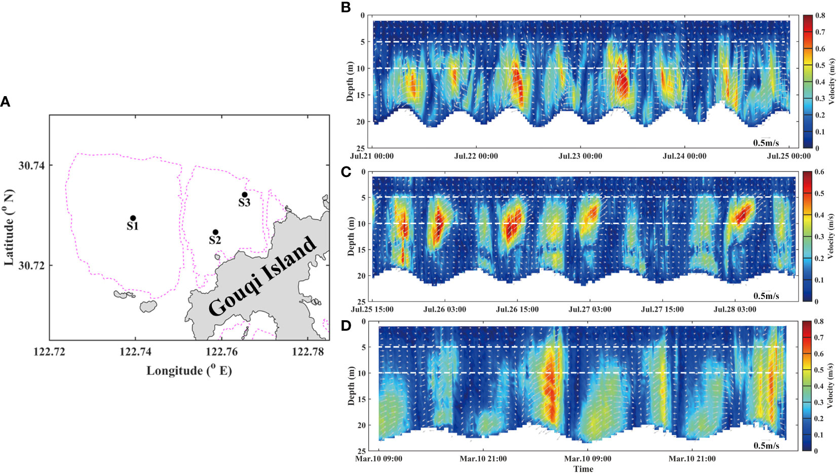
Figure 3 In-situ observed vertical profile of current collected by the ADCP mounted to a buoy for S1, S2 and S3 station. (A) Station location diagram. Time series of vertical current profile (B) at S1 during spring tide, from July 21, 2020 for 96 hours. (C) at S2 during neap tide, from July 25, 2020 for 72 hours. (D) at S3 during spring tide, from March 10, 2021 for 48 hours. The gray arrows indicate the horizontal direction and magnitude of tidal current.
S3 station is less affected by the farm since it is located at the edge of farm, the flow velocity of canopy layer thus reached 0.5 m/s during flood and ebb tide (Figure 3D). However, at S1 and S2 station located inside the farm, under the cumulative blockage influences of farm, the thickness of surface canopy boundary layer is maintained at about 5 m, and can be greater than 10 m when the hydrodynamic is weakened. The spatiotemporal variation of natural hydrodynamics environment in the aquaculture area cause significant spatiotemporal variation of surface canopy boundary layer thickness by suspended aquaculture facilities.
In addition to in-situ measurements, we also carried out a series of current measurements using ADCP mounted to a moving boat. The velocity profiles produced by suspended canopies such as mussel ropes and kelp may be divided into three layers: a bottom boundary layer, a canopy shear layer (i.e., a structure-induced boundary layer), and an internal canopy layer (Plew, 2011a; Cheng et al., 2019).The measured current profile outside and inside the farm (Figure 4) shows that the velocity is reduced in the upper water column, and the thickness of surface canopy boundary layer increased entering the farming area, up to about 10 m (Figure 4). The flow within the surface canopy boundary layer is attenuated by the drag force of suspended mussel farms.
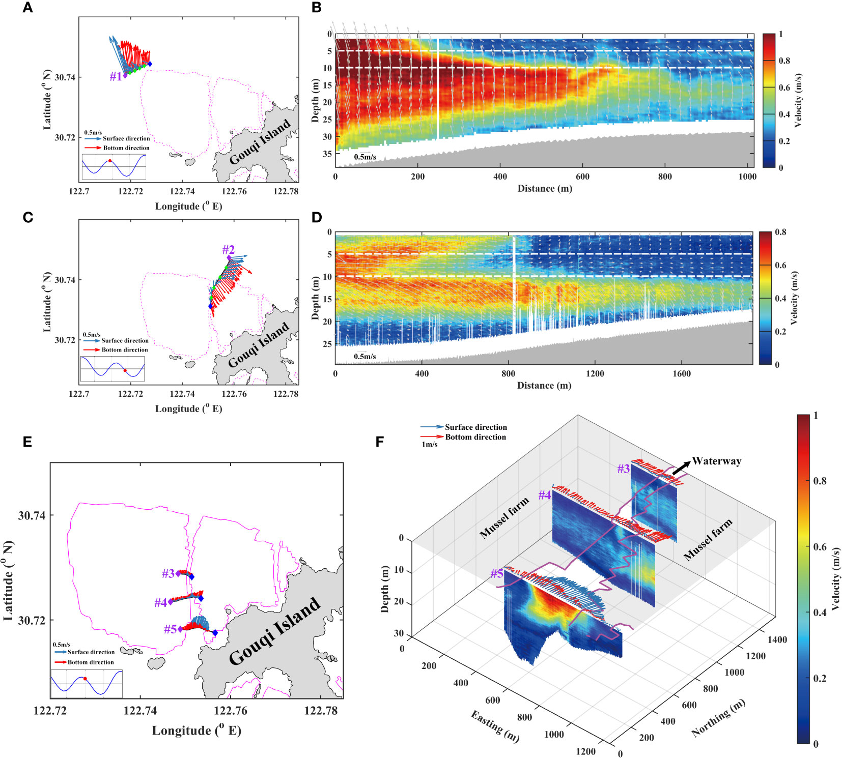
Figure 4 Observed vertical profiles of flow for transect lines #1, #2, #3, #4 and #5 collected by ADCP mounted to a boat. Pink lines indicate the borderlines of mussel farms. The insert plot is the time series of tidal elevation at Shengshan Tide station (122°28′E,30°43′N) with the red dot indicate the time instant of the tidal elevation. Blue and red arrows show the current vector at the surface and bottom, respectively. The gray arrows in (B, D) indicate the horizontal tidal current vector. The purple and blue diamond is the starting and end point of boat cruises respectively. The green diamonds in (A, C) indicate observation point of 400 meters intervals. (A) Transect line #1 & (C) Transect line #2 &(E) Transect line #3, #4 and #5 location diagram. (B) Vertical current profile along transect line #1 on July 10, 2021 during spring tide. (D) Vertical current profile along transect line #2 on June 29, 2021 during neap tide. (F) Vertical current profile along transect line #3, #4 and #5 on July 10, 2021 during spring tide within 30 minutes for 2 minutes, 4 minutes and 5 minutes, respectively.
A region of flow recirculation behind an object, a wake zone, may form downstream from the mussel farm (Plew et al., 2005; Plew et al., 2006; Cornejo et al., 2014; Tseung et al., 2015; Qiao, 2016), where lower velocity is present. The wake zone consists of, a steady wake zone with approximately constant velocity and a velocity recover zone where velocity increases downstream (Tseung et al., 2015). The results show that the wake zone occurred in the surface layer (Figure 4) with a thickness increasing closer to the farming area, up to 10 m.
In order to assess whether the current layout of central waterway in the north of Gouqi Island is suitable, we conducted three current profile observations from west to east along the waterway (Figure 4). The observed current profile at transect line #5 show that the horizontal velocity of the whole water column at the waterway is large with a maximum value of about 1m/s (Figure 4) due to the reduced cross section for flow to pass through by the farm. Due to the cumulative flow attenuation by the aquaculture facilities, the current at transect line #3 is smaller than that at line #4 which in turn is smaller than that at line #5 from south to north (Figure 4). The observations indicated that the spatiotemporal variation of natural hydrodynamic conditions around the farm have an important impact on that of tidal current within the farm. As a results, the hydrodynamic effect of large-scale aquaculture farm in the field has a sophisticated temporal and spatial variations.
Tidal elevation measurements at S4, S5, S6 and the Lvhua Tide Station were used to validate the model results. Skill score (SS) and correlation coefficient (CC) were calculated to quantify the model-data comparison.
where N is the number of samples for the time series, xm and xo are the predicted and observed tidal elevation respectively, and are the average of the variables.
The simulated and observed time series of tidal elevation at 4 stations are compared in Figure 5. Model performances quantified by SS and CC as follows: >0.65 excellent, 0.65–0.5 very good, 0.5–0.2 good, <0.2 poor (Wu et al., 2011). The root-mean-square error (RMSE) was also used to judge the accuracy of model results:
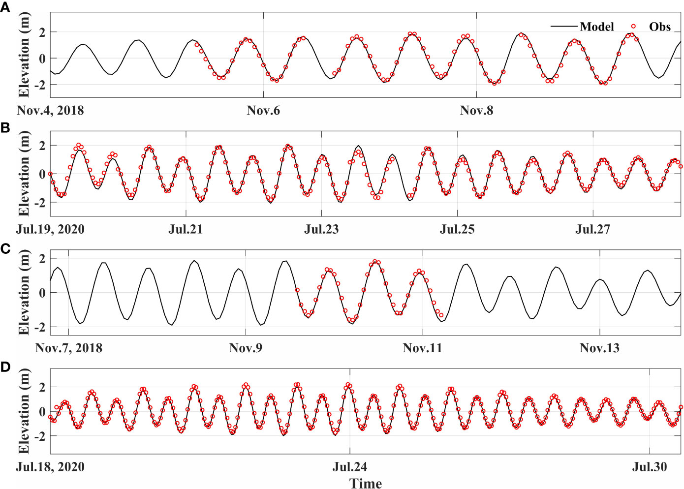
Figure 5 Model-data comparisons of tidal elevations at (A) S4 outside the farm, north of farm, (B) S5 outside the farm, south of Gouqi Island, (C) S6 north of Shengshan Island and (D) LvHua Tide Station (30°49′N, 122°36′E).
The SS and CC of model results are greater than 0.98 at all stations, and the RMSE is less than 0.2, which indicates that the simulated tidal elevations accurately reproduced the observed tidal elevations (Table 2).
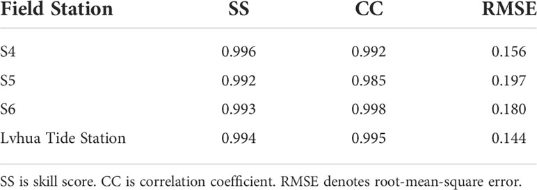
Table 2 The model-data comparisons of tidal elevation.
Simulated tidal currents were evaluated against observed data collected at S1 in the center of the mussel farm and S4 outside the mussel farm across the mussel farm (Figure 6). The skill score (SS), correlation coefficient (CC) and root-mean-square error (RMSE) are listed in Table 3. The SS and CC of surface and middle layer at S4 are both greater than 0.8 and the RMSE are less than 0.3, which are excellent scores. At S1, the model accuracies of middle and bottom layer are better than that of the surface layer. The SS and CC at S4 are better than those at S1 throughout the water column, whereas the RMSE at S1 is better than that of S4. The reason is probably that the surface layer flow velocity is consistently less than 0.2 m/s at S1 (Figure 7A), which is difficult to simulate.
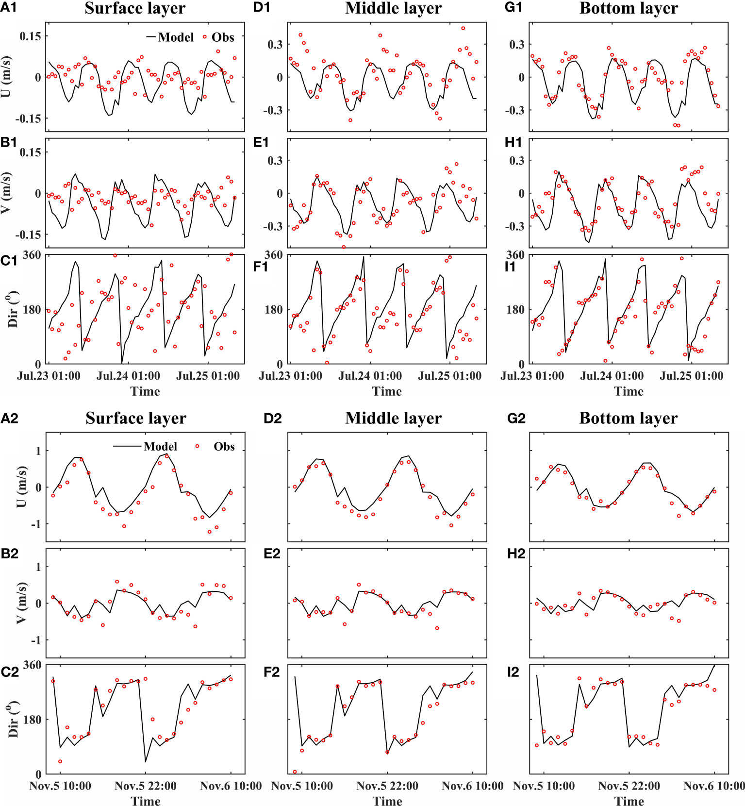
Figure 6 Model-data comparisons of tidal current velocity components and direction at S1 (A1-I1) inside the farm and S4 (A2-I2) outside the farm: (Upper) u in the x-direction, (Middle) v in the y-direction, (Lower) direction of current. (A–C) surface layer. (D–F) middle layer. (G–I) bottom layer.
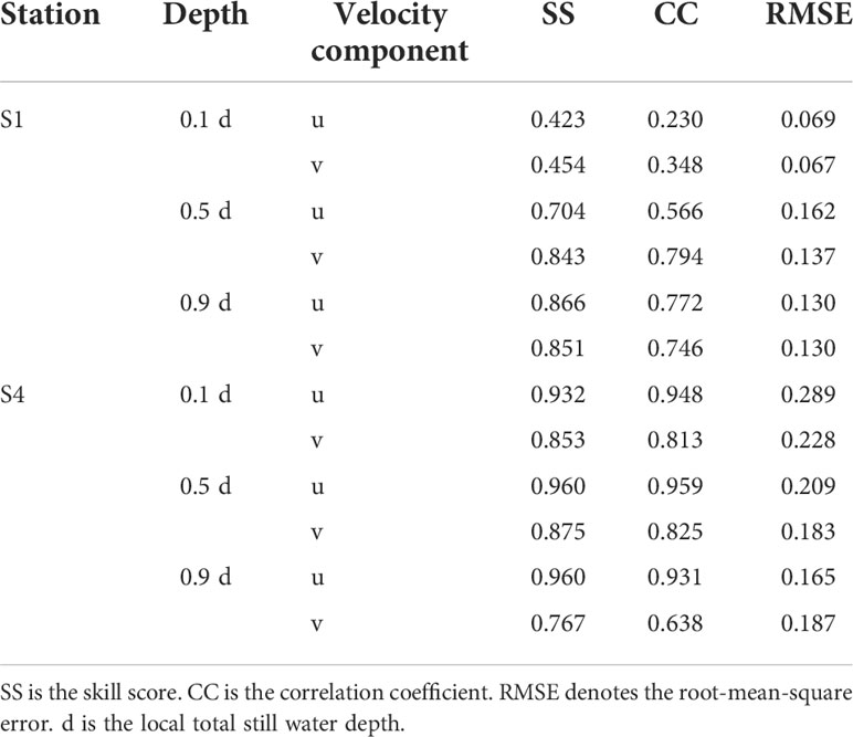
Table 3 The model-data comparisons of tidal current.
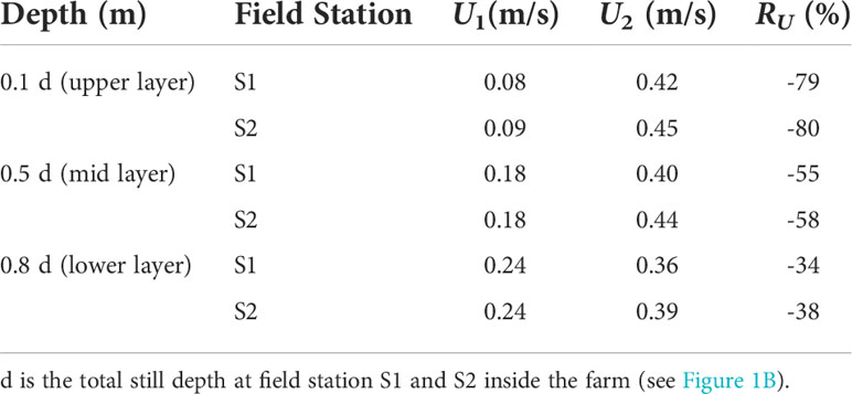
Table 4 The average relative difference of velocity RU (%) between with (U1) and without farm (U2).
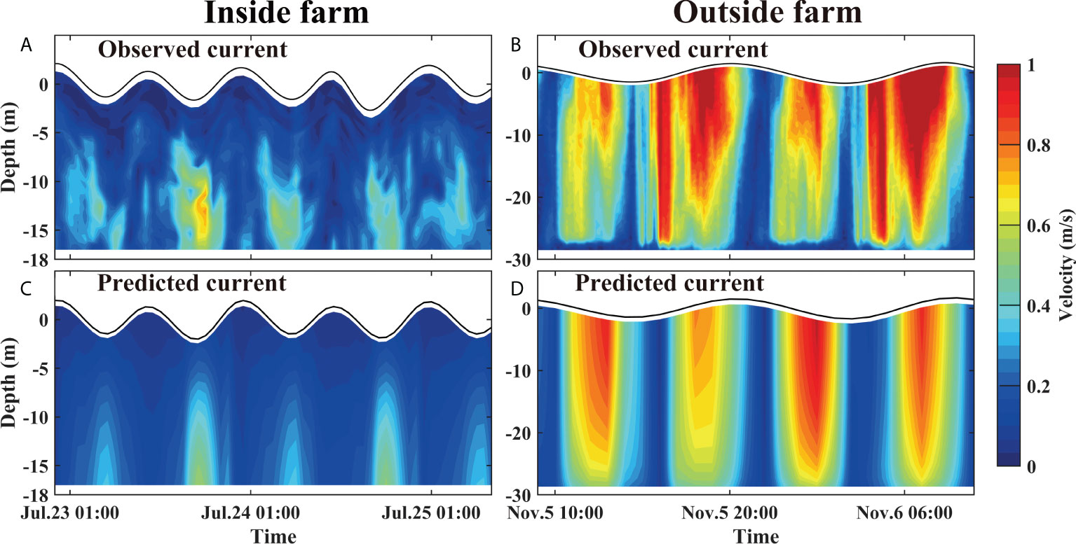
Figure 7 Model-data comparisons of time series of current profile at S1 station inside the farm (Left) and S4 station outside the farm (Right). (A) observed & (C) predicted current profile at S1. (B) observed & (D) predicted current profile at S4.
As stated previously, the effect of mussel farms was represented by assigning Wk and Lσ values individually to the sigma layers. The values of Wk and Lσ were determined by the field measurements. However, the horizontal spatial distribution of mussel farm is not uniform in the field, but limited by mesh resolution, the model cannot exactly represent each mussel farm. The mussel stocking density also have a significant influence on the flow field (Tseung et al., 2015; Xu and Dong, 2018). All these factors make the simulation of surface layer flow in the farm difficult.
The model results suggest that it is difficult to reproduce the complex three-dimensional flow structure inside suspended mussel farms using the present model. A CFD model such as that developed by Chen and Zou (2019) for fluid interaction with flexible suspended canopy are needed to fully resolve the 3D flow patterns within the farm. The flow pattern and its temporal variation, however, are well captured (Figure 7), thus the model can be used to study the hydrodynamic effects of large-scale suspended mussel farms around Gouqi Island. In addition, the simulation results demonstrate that the additional momentum sink term is suitable for modelling the effects of suspended mussel farms.
Large scale suspended mussel farms may attenuate the local ocean circulation considerably (Stevens et al., 2008; Campbell and Hall, 2019; Liu and Huguenard, 2020). The model is run with and without the mussel farms to assess the impacts of farms on the tidal currents. The tidal currents at depth = 0.1d where d is local water depth with and without farm during flood and ebb phase are shown in Figure 8.
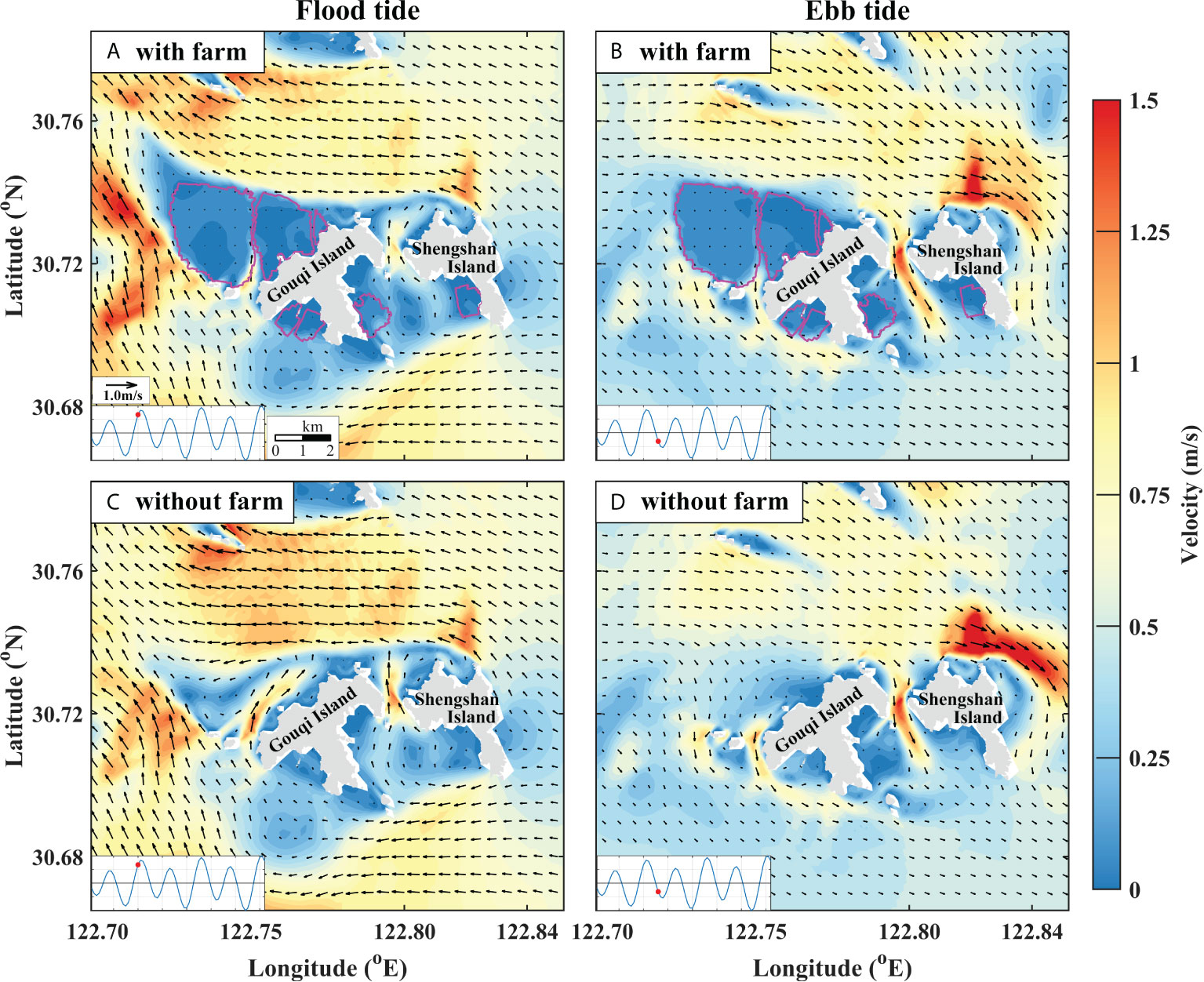
Figure 8 Predicted instantaneous surface layer (depth=0.1d, where d is local depth) flow field. (A, B) with and (C, D) without mussel farms during flood (Left) and ebb (Right) tide. The pink lines indicate the borderlines of the farm. The insert plot is the time series of the observed tidal elevation at Shengshan Tide station (122°28′E,30°43′N) with the red dot indicates the time instant of tidal elevation shown in the plot.
The main farm effect is the substantial reduction of surface flow during both flood and ebb tide. During flood tide, the tidal current from the east to the west at the north of Gouqi Island is weakened by the farm, whereas the tidal current from the southeast to the northwest at the west of the largest mussel farm is strengthened (Figures 8A, C). When the suspended mussel farms were removed, the tidal currents at the northeast of Shengshan Island and the west of Gouqi Island are strengthened, and the tidal currents at the middle of the islands is weakened (Figure 8C, D). The model results show that a wake zone appeared downstream from the farming area, the northwest of Gouqi Island during the flood tide (Figure 8A), under the combined influence of islands and aquaculture facilities. Therefore, we carried out moving-boat ADCP current profile observations (Figure 4) along a transect parallel to the coast of island outside the northwest farm during flood tide, when the tidal current direction is northwest that is consistent with the numerical results. These results indicate that the impact of suspended mussel farms is not limited to the immediate farm area, but extended to the local circulation outside the farms, which has significant implication on the ecosystem.
In order to quantify the degree of tidal current reduction around farms, the relative difference of tidal current velocity between with and without farm was evaluated by the following equation (Wu et al., 2014):
where U1 and U2 is the average tidal current velocity over tidal cycles of with farm and without farm. U is defined as:
where T is the averaging period (T = 58 days), A is the area of water layer, | u | is the magnitude of instantaneous tidal current velocity.
S1 and S2 stations inside the farm (see Figure 1B) were selected to represent the velocity change due to the mussel farms in water column (Table 4). The tidal current decrease is by more than 79%, 55% and 34% in the upper layer (depth=0.1d, where d is local water depth), middle layer (depth=0.5d) and lower layer (depth=0.8d) respectively, which is consistent with the previous study (Lin et al., 2016).
A harmonic analysis (T-Tide toolbox: Pawlowicz et al., 2002) for tidal currents of with and without farm case was conducted to obtain the amplitudes and phases of M2 (principal lunar semi-diurnal), S2 (principal solar semi-diurnal), K1 (lunar diurnal) and O1 (lunar diurnal) tidal constituents. Figure 9 presents the tidal ellipse at depth=0.1d where d is local water depth with and without farm. The semi major and minor axis of tidal ellipse represent the maximum and minimum current velocity within one period for the tidal constituent respectively. And the inclination of major and minor axis is equivalent to the orientation of the maximum and minimum current induced by each tidal constituent respectively.
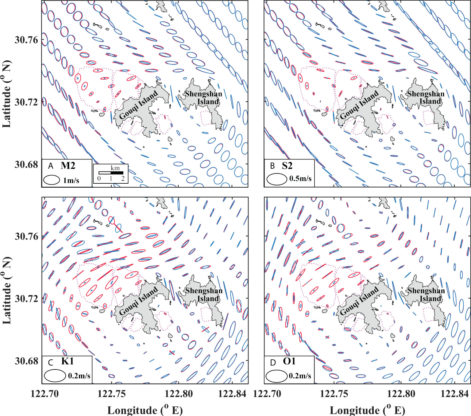
Figure 9 Modeled tidal ellipse in the surface layer (depth=0.1d, where d is local depth) with (blue) and without (red) farm. (A) M2 semi-tide. (B) S2 semi-tide. (C) K1 diurnal tide. (D) O1 diurnal tide. The pink dash lines indicate the borderlines of mussel farms.
M2 is the dominant tidal component around Gouqi Island. In the aquaculture farm at the north of Gouqi Island, without farm, the tidal current is in the southwest direction. At the edge of the farm, the tidal current gradually changes to the west direction, and so does S2 tidal constituent. The farm has little effect on the tidal current in the eastern area of Shengshan Island. The tidal ellipse of semidiurnal tide in the northeast area of Shengshan Island is almost perpendicular to that of diurnal tide. The semidiurnal tide comes from the southeast of the island, while that of diurnal tide comes from the northeast of the island. Due to the shelter effect of islands, the tides are divided into two branches, which lead to the complicated tidal currents around Gouqi Island.
The farm has a direct impact on the major axis and inclination of four tidal constituent ellipses, and its scope of influence can extend to a certain distance away from the farming area. The ellipse inclination variation of diurnal tide caused by the farm is greater than that of semidiurnal tide especially to the west of Gouqi Island (Figure 9). In case of K1, tidal constituent the blockage of farms changes the major axis of ellipse from northeast-southwest (NE-SW) to northwest-southeast (NW-SE) degenerating to rectilinear motion to the west of Gouqi Island (Figure 9C). Similar effects are observed for the O1 tidal constituent. (Figure 9D).
The variation of semidiurnal tides due to the farm is significantly enhanced within the farm but not so outside the farm (Figures 9A, B). The length of major axes is shortened inside the farm, and the reduction is the largest for the M2 tidal constituent. Besides, the influence of mussel farms on tides at the south of Gouqi Island is weaker than that at the north of Gouqi Island due to the fact that the former is weakened by the island with lower tidal current velocity, while the latter is adjacent to the open ocean with higher tidal current velocity.
The farm may affect both the magnitude and direction of the tidal current of the four tidal components which are both important for water transport. Therefore, in order to understand the major net water transport direction around Gouqi Island, the Euler residual tidal current was derived from model results. The Euler residual tidal current is derived an arithmetically averaged the tidal current to filter out the periodic oscillating component (Lee et al., 2017). In this study, the model results with and without farm for 58 days were averaged to obtain the Euler residual tidal current for surface layer (depth=0.1d where d is local water depth) and bottom layer (depth=0.8d). The Euler residual tidal current of with and without farm were presented in Figure 10.
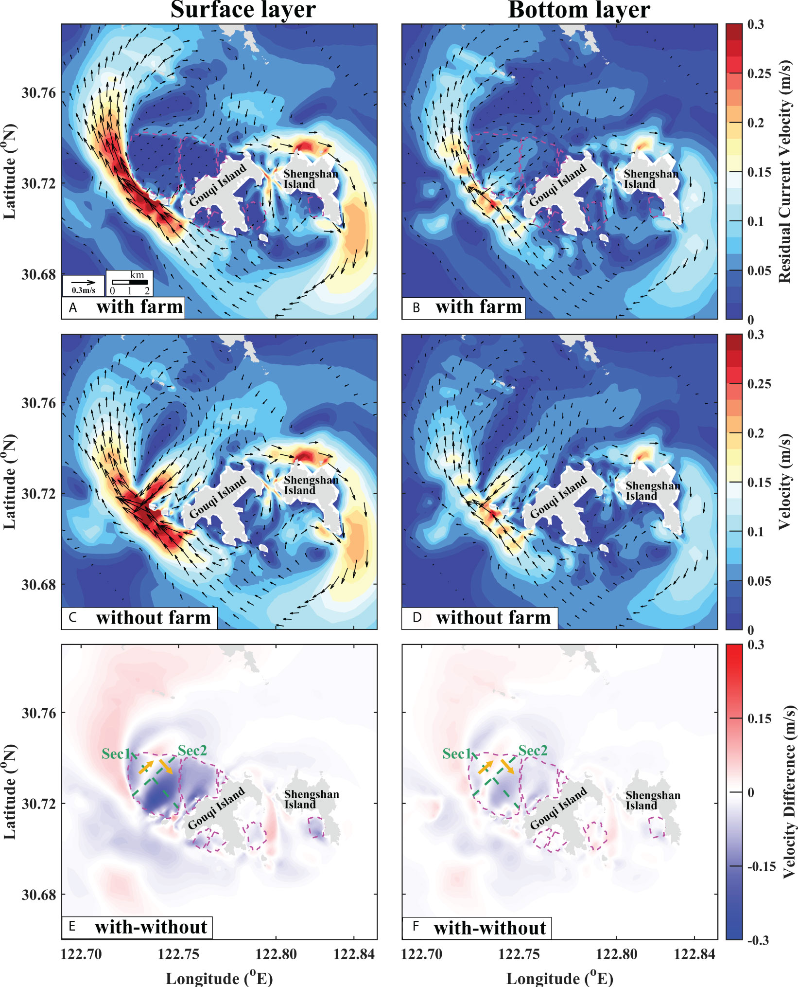
Figure 10 Modeled Eulerian residual tidal current. (A, B) with and (C, D) without mussel farms at the surface (Left, depth=0.1d, where d is local depth) and bottom (Right, depth=0.8d) layer. (E, F) is the difference of residual current with and without farm at the surface (Left) and bottom (Right) layer. The orange arrows show the positive direction of water transport across Sec1 and Sec2 in the figure. Pink dash lines indicate the borderlines of mussel farms.
With farm, a major residual current transport is observed around the farm, the northwest of Gouqi Island flowing from southeast (SE) to northwest (NW) (Figure 10A). Without farm, an additional residual current transport is observed flowing from northeast (NE) to southwest (SW) within the farm at the north of Gouqi Island (Figure 10C). The NE to SW residual tidal current also appears in the bottom layer with and without farm but the latter is stronger than that of the former (Figure 10B). The direction of the two residual tidal current is perpendicular to each other, and the magnitude of the residual tidal current outside the farm is greater than that inside the farm (Figures 10C, D). The presence of farm not only weaken the surface and bottom residual transport inside the farm, but also strengthened the residual transport at the north of the farm (Figure 10E). Moreover, the bottom layer residual transport is also strengthened inside the farm (Figure 10F). Overall, it is evident that the presence of mussel farms intensifies the residual transport in the SE to NW direction but weakens that in the NE to SW direction (Figures 10E, F).
Based on the residual transport pattern, Sec1 and Sec2 (see Figures 10E, F) were set up to estimate the change in the net water flux in the aquaculture area by the presence of farm. The Sec1 cuts the largest farm into almost two halves from SE to NW with a length of 3.6 km, and the Sec2 cuts the largest farm into two halves from NE to SW with a length of 3 km. The time evolution of water flux and the sum of the water flux along two transects over a month calculated by the Eq. (1) and (2) were shown in Figure 11.
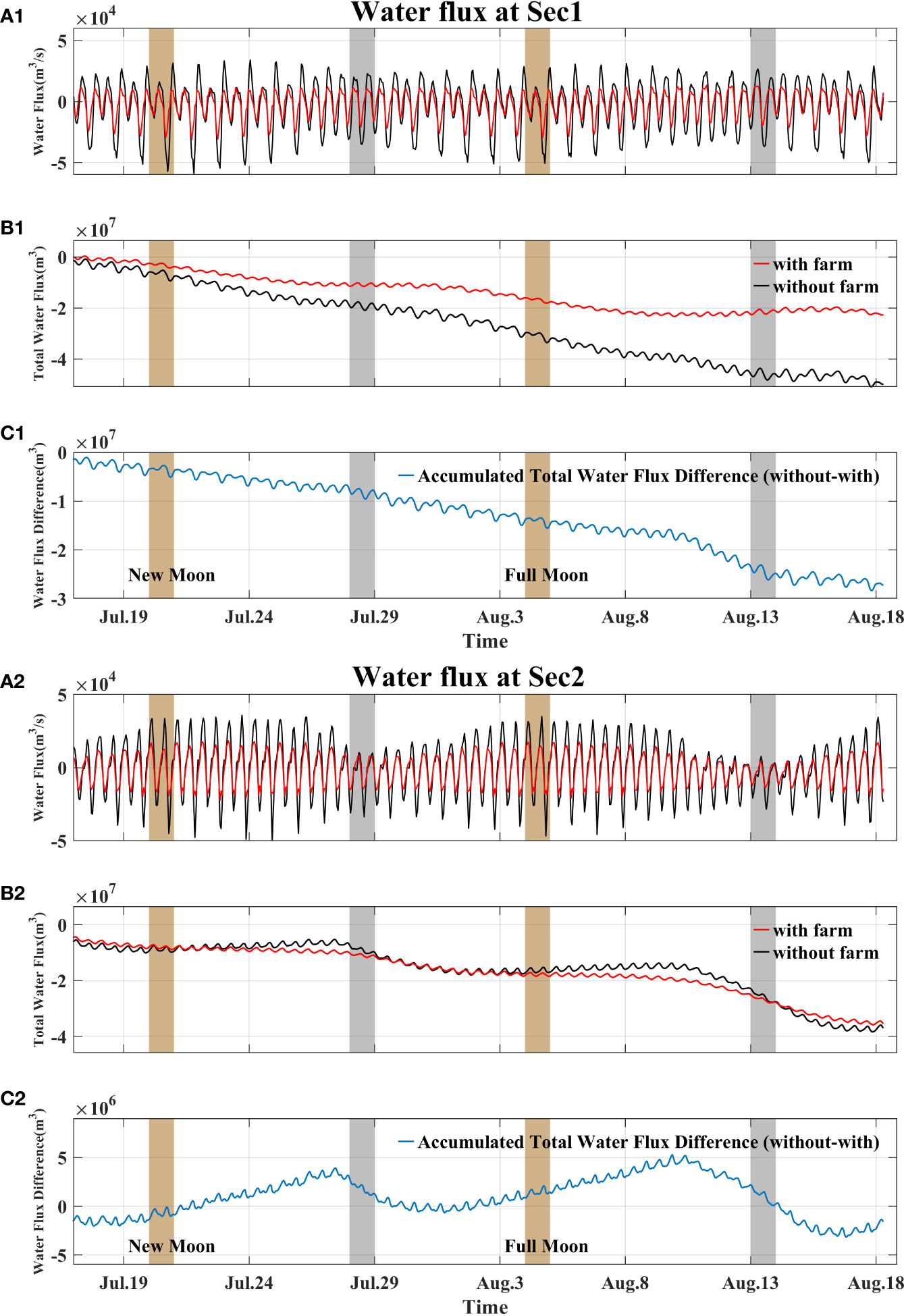
Figure 11 Water flux through Sec1 (A1-C1) and Sec2 (A2-C2). (A) water flux with (red) and without (black) farm. (B) accumulated total water flux with (red) and without (black) farm. (C) difference of total water flux with and without farm. The brown and grey box indicate time interval of 24 hours during spring and neap tide, respectively.
The time series of water flux (Figure 11) through two transects have a semidiurnal periodicity. The maximum water flux with farm through Sec1 are 2.9×10⁴ m3 s-1 and 2.0×10⁴ m3 s-1 during spring and neap tides, respectively. Without farm, the maximum water flux through Sec1 is 5.7 ×10⁴ m3 s-1 during spring tide, indicating the farm reduce the water flux by~ 49%. The water flux with farm through Sec2 is ~ 1.9 ×10⁴ m3 s-1 and 0.4 ×10⁴ m3 s-1 during spring and neap tides respectively, smaller than that at Sec1. The maximum water flux without farm through Sec2 is 4.6 ×10⁴ m3 s-1 during spring tide, indicating the farm reduce the water flux by ~59%, greater than that at Sec1.
The total water flux over a month at Sec1 is negative with and without farm showing a NE to SW transport (Figure 11), which is consistent with the direction of residual currents in Figure 10. The maximum difference in the total water flux over a month with and without farm at Sec1 can reach 2.8×10⁷ m3 (Figure 11). The total water flux at Sec1 indicates that the farm greatly alters the amount of water transport, but not the main direction of water transport. The total water flux over a month at Sec2 with and without farm is also negative indicating offshore transport from SE to NW (Figure 11). The maximum difference in total water flux over a month with and without farm at Sec2 is 5.2×10⁶ m3, smaller than that of at Sec1 (Figure 11). The total water flux difference over a month displays a semi-lunar periodicity at Sec2 but not at Sec1 (Figure 11). The total water flux difference over a month at Sec2 is positive during the transition between spring and neap tide with a maximum before neap tide, but become negative during the transition between neap and spring tide. This is likely due to the enhanced bottom layer tidal current shown in Figure 10F.
Several studies have established a comprehensive decision-making system for key aquaculture strategies (Ferreira et al., 2008; Ferreira et al., 2009; Ibarra et al., 2014; Konstantinou and Kombiadou, 2020), such as farm layout, optimized stocking density, and carrying capacity estimation, which is critical for overall farm production. Neglecting farm drag may underestimate seston depletion within the farm (Plew, 2011b; O’Donncha et al., 2013), and overestimate of carrying capacity. As a result, the hydrodynamic effect of large-scale aquaculture facilities is critical for aquaculture decision-making.
The farm is a suspended canopy made of distributed elements that act as a porous media to flow. Flow disturbances of suspended canopy generally presents reduced flow velocity within the canopy, and increased flow beneath the canopy (Plew et al., 2005; Plew, 2011a; Newell and Richardson, 2014; Wu et al., 2014; Wu et al., 2022; Qiao, 2016; O’Donncha et al., 2017). Due to differences in geographic environment, faming size, farm layout and species farmed, the current velocity decrease in the canopy layer varies from farm to farm. For kelp farms, the reduction of average surface current velocity is around 40% in a bay (Shi et al., 2011). As little as 25% reduction of current within the suspended canopy have been found (O’Donncha et al., 2013; Hulot et al., 2020).
The thickness of the canopy shear layer is proportional to the drag force induced by the aquaculture facilities and the depth ratios (canopy length to water depth) (Plew, 2011a; Qiao, 2016). Our field observations revealed the presence of a surface canopy boundary layer inside the farm. And its thickness progressively increase with increasing distance downstream. Given the relatively intense aquaculture density (4 m2 sleeve-1) on Gouqi Island, this is mainly due to the cumulative effect of flow attenuation by the farming facilities. The surface canopy boundary layer can also be seen in a large-scale suspended cage fish farm of ~ 300 km2 at Sansha Bay (Lin et al., 2019; Jiang et al., 2022), where cage-induced drag on the flow field may reach a depth up to 20 m in rather deep channels (30~40 m).
The tidal ellipse results described above in section 5.2 provides guidance for farm-scale layout optimization. For example, within the farm, the orientation of the aquaculture facilities shall be parallel to the major axis of the tidal ellipse, i.e., the direction of flood and ebb tides, in order to minimize the flow resistance of the farm, and therefore increase the water exchange rate. The moving-boat ADCP observations of current profile throughout the waterway indicate the same strategy (Figure 4F). Strong current is observed on the east side of transect #4, and that the ebb flow direction is southwest, which is consistent with the findings of tidal ellipses. The waterway channel’s primary function right now is to make it easier for ships and fisherman to operate on the farm. On the other hand, the channel is a crucial passage for off-site replenishment of high biomass water, supplying food for mussel. Therefore, the layout of waterway should minimize the blockage effect of aquaculture facility, so that the high biomass seawater outside the farm can be transported into the farming area in time for the mussel growth, thereby improving the production and quality of aquaculture. This shall be taken into account for farm unit layout design in the future.
The major goal of this paper is to use field measurements and numerical models to investigate the hydrodynamic effects by a large-scale suspended mussel farm. In order to incorporate the blockage effects of aquaculture facility into large scale ocean models, such as ECOM-si, an appropriate drag coefficient of the suspended mussel farms is necessary. In this study, the drag coefficient is chosen based on the previous study (Beudin et al., 2017; Liu and Huguenard, 2020). Thus, more studies are required to provide improved drag coefficients through small scale computational fluid dynamics (CFD) simulations such as those of Chen & Zou (2019), field observations and laboratory experiments. Furthermore, the impacts of aquaculture facilities on tides are the main concern of this study, other physical processes such as stratification, turbulent mixing, and waves (Plew et al., 2006; Stevens and Petersen, 2011; Zhu et al., 2020)-are the subjects of future research. To determine the ideal distance between farm blocks, it is also important to consider how aquaculture farms may affect the primary production of the surrounding sea area which will be the worthwhile future works.
The influence of mussel farms on the flow structures near Gouqi Island was investigated using a three-dimensional ocean model and field observations. Model-data comparisons show that the additional sink terms in the momentum equations of ECOM-si adequately capture the blocking effect of large-scale suspended mussel farms. Comparisons of model results with and without farms indicate that the presence of mussel farms reduces the velocity by more than 79%, 55% and 34% in the upper, the middle, and the bottom layer at the center of farms, respectively. Tidal harmonic analysis demonstrate that mussel farms affect both the major axis and inclination of four major tidal constituent ellipses (M2, S2, K1 and O1) at much larger area than the farm area. The farm reduces the velocity magnitude of semidiurnal tide, but change both the magnitude and direction of diurnal tide, as well.
The residual currents from nonlinear interactions of tidal currents play a key role in the transport of material, such as seston and sediment. The SE to NW surface residual flow along the west border of the farm is strengthened, while the NE to SW surface residual flow inside the farm is weakened. To quantify the residual current around the farm, two cross sections, Sec 1 and Sec 2 are selected and they are perpendicular to the two major residual current and cut through the center of the farm. Sec 1 cuts the largest farm into two halves from SE to NW with a length of 3.6 km, and the Sec 2 cuts the largest farm into two halves from NE to SW with a length of 3 km. The water flux reduction by mussel farms through Sec1 and Sec2 can reach 49% and 59% respectively. In addition, the difference in the total water flux at Sec1 with and without farms reaches up to 2.8×10⁷ m3 with the major water transport direction in NE to SW. At Sec2, the total water flux difference displays a semi-lunar periodicity, positive during the transition from spring to neap tide and negative during the transition from neap to spring tide. The total offshore water transport at Sec2 may be increased by mussel farms by up to 5.2×10⁶ m3, an order of magnitude smaller than that of at Sec1.
The field observation revealed tidal asymmetry in the farm at the north of Gouqi Island. The flood currents are stronger than the ebb currents at field station S1 inside the farm and S3, while the opposite is true at field station S2 inside the farm. The thickness of the surface canopy boundary layer formed by suspended mussel farms has large spatiotemporal variations due to the heterogeneity in natural hydrodynamics within the farm. The observed current velocity profiles show that the thickness of the surface canopy boundary layer is maintained at about 5 m inside the farm, but may become larger than 10 m when the hydrodynamic is weakened by the cumulative blocking effect. And a wake zone was observed downstream the northwest farming area, which becomes larger closer to the farming area.
The present model can be a robust tool for farm site selection or farm extension and configuration by estimating the hydrodynamic changes by mussel farm and guide the production management decisions. The mussel farm needs to comply with the natural hydrodynamic conditions at the site and minimize the blocking effect on the water exchange between the water body inside and outside the farm, so that the suspended particulate organic matter in the farm can be replenished in time, which is essential for healthy mussel growth.
The raw data supporting the conclusions of this article will be made available by the authors, without undue reservation.
WZ and YW conducted the numerical experiments and wrote the first draft of the manuscript. QZ and WZ analyzed the results and revised the manuscript. WY and GY collected and analyzed the field observation data. JL conceived the idea, designed the experiments, and revised the manuscript. All authors contributed extensively to the interpretation of results and approved the submitted version.
This research was supported by National Key R&D Program of China (2018YFD0900905 and 2019YFD0901302). This study was also funded by the project of “Study on the germplasm, environment and culture strategy of mussel culture in sea area around Gouqi Island”, Shengsi County, Zhejiang Province.
The authors thank Changsheng Chen, Jianrong Zhu and Hui Wu for their generosity allowing us to use the modified ECOM-si model. We thank Hidekatsu Yamazaki and Hui Wu for their comments on the content. The authors acknowledge Xingchen Wu, Yiguo Tan, Mingbo Sun and Jianshi Liu for deploying and retrieving the instruments used in this investigation.
The authors declare that the research was conducted in the absence of any commercial or financial relationships that could be construed as a potential conflict of interest.
All claims expressed in this article are solely those of the authors and do not necessarily represent those of their affiliated organizations, or those of the publisher, the editors and the reviewers. Any product that may be evaluated in this article, or claim that may be made by its manufacturer, is not guaranteed or endorsed by the publisher.
Aguiar E., Piedracoba S., Alvarez-Salgado X. A., Labarta U. (2015). Circulation of water through a mussel raft: clearance area vs. idealized linear flows. Rev. Aquacul. 9, 3–22. doi: 10.1111/raq.12099
Anaïs A., Adélaïde A., Jean-Claude G., Oihana L., Philippe A., Nabila G. (2020). Assessment of carrying capacity for bivalve mariculture in subtropical and tropical regions: the need for tailored management tools and guidelines. Rev. Aquacult., 12, 1721–1735. doi: 10.1111/raq.12406
Beudin A., Kalra T. S., Ganju N. K., Warner J. C. (2017). Development of a coupled wave-flow-vegetation interaction model. Comput. Geosci. 100, 76–86. doi: 10.1016/j.cageo.2016.12.010
Blumberg A. (1994). A primer for ECOM-si. technical report of HydroQual, Vol. 66. Mahwah N.J.: Technical Report of HydroQual.
Broch O. J., Klebert P., Michelsen F. A., Alver M. O. (2020). Multiscale modelling of cage effects on the transport of effluents from open aquaculture systems. PloS One 15, e0228502. doi: 10.1371/journal.pone.0228502
Byron C., Link J., Costa-Pierce B., Bengtson D. (2011a). Calculating ecological carrying capacity of shellfish aquaculture using mass-balance modeling: Narragansett bay, Rhode island. Ecol. Model. 222, 1743–1755. doi: 10.1016/j.ecolmodel.2011.03.010
Byron C., Link J., Costa-Pierce B., Bengtson D. (2011b). Modeling ecological carrying capacity of shellfish aquaculture in highly flushed temperate lagoons. Aquaculture 314, 87–99. doi: 10.1016/j.aquaculture.2011.02.019
Campbell M. D., Hall S. G. (2019). Hydrodynamic effects on oyster aquaculture systems: a review. Rev. Aquacult. 11, 896–906. doi: 10.1111/raq.12271
Cheng W., Sun Z., Liang S. (2019). Numerical simulation of flow through suspended and submerged canopy. Adv. Water Resour. 127, 109–119. doi: 10.1016/j.advwatres.2019.01.008
Chen H., Zou Q.-P. (2019). Eulerian–Lagrangian flow-vegetation interaction model using immersed boundary method and OpenFOAM. Adv. Water Resour. 126, 176–192. doi: 10.1016/j.advwatres.2019.02.006
Cornejo P., Sepúlveda H. H., Gutiérrez M. H., Olivares G. (2014). Numerical studies on the hydrodynamic effects of a salmon farm in an idealized environment. Aquaculture 430, 195–206. doi: 10.1016/j.aquaculture.2014.04.015
Delaux S., Stevens C. L., Popinet S. (2011). High-resolution computational fluid dynamics modelling of suspended shellfish structures. Environ. Fluid. Mech. 11, 405–425. doi: 10.1007/s10652-010-9183-y
Duarte P., Alvarez-Salgado X. A., Fernández-Reiriz M. J., Piedracoba S., Labarta U. (2014). A modeling study on the hydrodynamics of a coastal embayment occupied by mussel farms (Ria de Ares-betanzos, NW Iberian peninsula). Estuar. Coast. Shelf. Sci. 147, 42–55. doi: 10.1016/j.ecss.2014.05.021
FAO (2020). The state of world fisheries and aquaculture 2020 Sustainability in action. (Rome). doi: 10.4060/ca9229en
Ferreira J. G., Hawkins A. J. S., Monteiro P., Moore H., Service M., Pascoe P. L., et al. (2008). Integrated assessment of ecosystem-scale carrying capacity in shellfish growing areas. Aquaculture 275, 138–151. doi: 10.1016/j.aquaculture.2007.12.018
Ferreira J. G., Sequeira A., Hawkins A. J. S., Newton A., Nickell T. D., Pastres R., et al. (2009). Analysis of coastal and offshore aquaculture: Application of the FARM model to multiple systems and shellfish species. Aquaculture 289, 32–41. doi: 10.1016/j.aquaculture.2008.12.017
Filgueira R. (2018). Identifying the optimal depth for mussel suspended culture in shallow and turbid environments. J. Sea. Res. 132, 15–23. doi: 10.1016/j.seares.2017.11.006
Filgueira R., Comeau L. A., Guyondet T., McKindsey C. W., Byron C. J. (2015). “Modelling carrying capacity of bivalve aquaculture: A review of definitions and methods,” in Encyclopedia of sustainability science and technology. Ed. Meyers R. A. (New York, NY: Springer New York), 1–33. doi: 10.1007/978-1-4939-2493-6_945-1
Froján M., Castro C. G., Zúñiga D., Arbones B., Alonso-Pérez F., Figueiras F. G. (2018). Mussel farming impact on pelagic production and respiration rates in a coastal upwelling embayment (Ría de vigo, NW Spain). Estuar. Coast. Shelf. Sci. 204, 130–139. doi: 10.1016/j.ecss.2018.02.025
Gao Y., Fang J., Lin F., Li F., Li W., Wang X., et al. (2020). Simulation of oyster ecological carrying capacity in sanggou bay in the ecosystem context. Aquacul. Int. 28, 2059–2079. doi: 10.1007/s10499-020-00576-3
Garlock T., Asche F., Anderson J., Bjørndal T., Kumar G., Lorenzen K., et al. (2019). A global blue revolution: Aquaculture growth across regions, species, and countries. Rev. Fish. Sci. Aquacul. 28, 107–116. doi: 10.1080/23308249.2019.1678111
Grant J., Bacher C. (2001). A numerical model of flow modification induced by suspended aquaculture in a Chinese bay. Can. J. Fish. Aquat. Sci. 58, 1003–1011. doi: 10.1139/f01-027
Hulot V., Saulnier D., Lafabrie C., Gaertner-Mazouni N. (2020). Shellfish culture: a complex driver of planktonic communities. Rev. Aquacult. 12, 33–46. doi: 10.1111/raq.12303
Ibarra D. A., Fennel K., Cullen J. J. (2014). Coupling 3-d eulerian bio-physics (ROMS) with individual-based shellfish ecophysiology (SHELL-e): A hybrid model for carrying capacity and environmental impacts of bivalve aquaculture. Ecol. Model. 273, 63–78. doi: 10.1016/j.ecolmodel.2013.10.024
Jiang X., Tu J., Fan D. (2022). The influence of a suspended cage aquaculture farm on the hydrodynamic environment in a semienclosed bay, SE China. Front. Mar. Sci. 8. doi: 10.3389/fmars.2021.779866
Konstantinou Z. I., Kombiadou K. (2020). Rethinking suspended mussel-farming modelling: Combining hydrodynamic and bio-economic models to support integrated aquaculture management. Aquaculture 523, 735179. doi: 10.1016/j.aquaculture.2020.735179
Konstantinou Z. I., Kombiadou K., Krestenitis Y. N. (2015). Effective mussel-farming governance in Greece: Testing the guidelines through models, to evaluate sustainable management alternatives. Ocean. Coast. Manage. 118, 247–258. doi: 10.1016/j.ocecoaman.2015.05.011
Lee S. B., Li M., Zhang F. (2017). Impact of sea level rise on tidal range in Chesapeake and Delaware bays. J. Geophys. Res. Ocean. 122, 3917–3938. doi: 10.1002/2016JC012597
Li X., Li M., McLelland S. J., Jordan L.-B., Simmons S. M., Amoudry L. O., et al. (2017). Modelling tidal stream turbines in a three-dimensional wave-current fully coupled oceanographic model. Renewable Energy 114, 297–307. doi: 10.1016/j.renene.2017.02.033
Lin H., Chen Z., Hu J., Cucco A., Sun Z., Chen X., et al. (2019). Impact of cage aquaculture on water exchange in sansha bay. Cont Shelf. Res. 188, 103963. doi: 10.1016/j.csr.2019.103963
Lin J., Li C., Boswell K. M., Kimball M., Rozas L. (2015). Examination of winter circulation in a northern gulf of Mexico estuary. Estuar Coast. 39, 879–899. doi: 10.1007/s12237-015-0048-y
Lin J., Li C., Zhang S. (2016). Hydrodynamic effect of a large offshore mussel suspended aquaculture farm. Aquaculture 451, 147–155. doi: 10.1016/j.aquaculture.2015.08.039
Liu Z., Huguenard K. (2020). Hydrodynamic response of a floating aquaculture farm in a low inflow estuary. J. Geophys. Res.: Ocean. 125, e2019JC015625. doi: 10.1029/2019jc015625
Mascorda Cabre L., Hosegood P., Attrill M. J., Bridger D., Sheehan E. V. (2021). Offshore longline mussel farms: a review of oceanographic and ecological interactions to inform future research needs, policy and management. Rev. Aquacul. 13, 1864–1887. doi: 10.1111/raq.12549
Mustafa S., Estim A., AI-Azad S., Shaleh S. R. M., Shapawi R. (2017). Aquaculture sustainability: Multidisciplinary perspectives and adaptable models for seafood security. J. Fish. Aquacul. Dev. 126. doi: 10.29011/JFAD-126/100026
Newell C. R., Richardson J. (2014). The effects of ambient and aquaculture structure hydrodynamics on the food supply and demand of mussel rafts. J. Shellfish. Res. 33, 257–272. doi: 10.2983/035.033.0125
O’Donncha F., Hartnett M., Nash S. (2013). Physical and numerical investigation of the hydrodynamic implications of aquaculture farms. Aquacul. Eng. 52, 14–26. doi: 10.1016/j.aquaeng.2012.07.006
O’Donncha F., Hartnett M., Plew D. R. (2015). Parameterizing suspended canopy effects in a three-dimensional hydrodynamic model. J. Hydraulic. Res. 53, 714–727. doi: 10.1080/00221686.2015.1093036
O’Donncha F., James S. C., Ragnoli E. (2017). Modelling study of the effects of suspended aquaculture installations on tidal stream generation in cobscook bay. Renewable Energy 102, 65–76. doi: 10.1016/j.renene.2016.10.024
O’Hara Murray R., Gallego A. (2017). A modelling study of the tidal stream resource of the pentland firth, Scotland. Renewable Energy 102, 326–340. doi: 10.1016/j.renene.2016.10.053
Pawlowicz R., Beardsley B., Lentz S. (2002). Classical tidal harmonic analysis including error estimates in MATLAB using T_TIDE. Comput. Geosci. 28, 929–937. doi: 10.1016/S0098-3004(02)00013-4
Plew D. R. (2011a). Depth-averaged drag coefficient for modeling flow through suspended canopies. J. Hydraul. Eng. 137, 234–247. doi: 10.1061/(ASCE)HY.1943-7900.0000300
Plew D. R. (2011b). Shellfish farm-induced changes to tidal circulation in an embayment, and implications for seston depletion. Aquacul. Environ. Interact. 1, 201–214. doi: 10.3354/aei00020
Plew D. R., Spigel R. H., Stevens C. L., Nokes R. I., Davidson M. J. (2006). Stratified flow interactions with a suspended canopy. Environ. Fluid. Mech. 6, 519–539. doi: 10.1007/s10652-006-9008-1
Plew D. R., Stevens C. L., Spigel R. H., Hartstein N. D. (2005). Hydrodynamic implications of Large offshore mussel farms. IEEE J. Ocean. Eng. 30, 95–108. doi: 10.1109/joe.2004.841387
Qiao J. D. (2016). Flow structure and turbulence characteristics downstream of a spanwise suspended linear array. Environ. Fluid. Mech. 16, 1021–1041. doi: 10.1007/s10652-016-9465-0
Reid G. K., Dumas A., Chopin T. B. R. (2020). Performance measures and models for open-water integrated multi-trophic aquaculture. Rev. Aquacul. 12, 47–75. doi: 10.1111/raq.12304
Roc T., Conley D. C., Greaves D. (2013). Methodology for tidal turbine representation in ocean circulation model. Renewable Energy 51, 448–464. doi: 10.1016/j.renene.2012.09.039
Shi J., Wei H. (2009). Simulation of hydrodynamic structures in a semi-enclosed bay with dense raft-culture. Periodic. Ocean. Univ. China (Chinese) 39, 1181–1187. doi: 10.16441/j.cnki
Shi J., Wei H., Zhao L., Yuan Y., Fang J., Zhang J. (2011). A physical–biological coupled aquaculture model for a suspended aquaculture area of China. Aquaculture 318, 412–424. doi: 10.1016/j.aquaculture.2011.05.048
Stevens C., Petersen J. (2011). Turbulent, stratified flow through a suspended shellfish canopy: implications for mussel farm design. Aquacult. Environ. Interact. 2, 87–104. doi: 10.3354/aei00033
Stevens C., Plew D., Hartstein N., Fredriksson D. (2008). The physics of open-water shellfish aquaculture. Aquacul. Eng. 38, 145–160. doi: 10.1016/j.aquaeng.2008.01.006
Tseung H. L., Kikkert G. A., Plew D. (2015). Hydrodynamics of suspended canopies with limited length and width. Environ. Fluid. Mech. 16, 145–166. doi: 10.1007/s10652-015-9419-y
Wu Y., Chaffey J., Law B., Greenberg D. A., Drozdowski A., Page F., et al. (2014). A three-dimensional hydrodynamic model for aquaculture: a case study in the bay of fundy. Aquacul. Environ. Interact. 5, 235–248. doi: 10.3354/aei00108
Wu H., Zhu J. (2010). Advection scheme with 3rd high-order spatial interpolation at the middle temporal level and its application to saltwater intrusion in the changjiang estuary. Ocean. Model. 33, 33–51. doi: 10.1016/j.ocemod.2009.12.001
Wu H., Zhu J., Chen B., Chen Y. (2006). Quantitative relationship of runoff and tide to saltwater spilling over from the north branch in the changjiang estuary: A numerical study. Estuar. Coast. Shelf. Sci. 69, 125–132. doi: 10.1016/j.ecss.2006.04.009
Wu H., Zhu J., Shen J., Wang H. (2011). Tidal modulation on the changjiang river plume in summer. J. Geophys. Res. 116, C08017. doi: 10.1029/2011jc007209
Wu Y., Law B., Ding F., Flaherty-Sproul M.O. (2022). Modeling the effect of cage drag on particle residence time within fish farms in the Bay of Fundy. Aquac Environ Interact. 14, 163–179.
Xu T.-J., Dong G.-H. (2018). Numerical simulation of the hydrodynamic behaviour of mussel farm in currents. Ship. Offshore. Struct. 13, 835–846. doi: 10.1080/17445302.2018.1465380
Yang Z., Wang T., Copping A. E. (2013). Modeling tidal stream energy extraction and its effects on transport processes in a tidal channel and bay system using a three-dimensional coastal ocean model. Renewable Energy 50, 605–613. doi: 10.1016/j.renene.2012.07.024
Zhang Q., Li C., Huang W., Lin J., Hiatt M., Rivera-Monroy V. H. (2022). Water circulation driven by cold fronts in the wax lake delta (Louisiana, USA). JMSE 10, 415. doi: 10.3390/jmse10030415
Zhang S. Y., Wang L., Wang W. D. (2008). Algal communities at gouqi island in the zhoushan archipelago, China. J. Appl. Phycol. 20, 853–861. doi: 10.1007/s10811-008-9338-0
Keywords: suspended mussel aquaculture, blocking effect, momentum sink, ECOM-si, drag of canopy
Citation: Zhong W, Lin J, Zou Q, Wen Y, Yang W and Yang G (2022) Hydrodynamic effects of large-scale suspended mussel farms: Field observations and numerical simulations. Front. Mar. Sci. 9:973155. doi: 10.3389/fmars.2022.973155
Received: 19 June 2022; Accepted: 25 July 2022;
Published: 23 August 2022.
Edited by:
Houshuo Jiang, Woods Hole Oceanographic Institution, United StatesReviewed by:
Andrea Cucco, National Research Council (CNR), ItalyCopyright © 2022 Zhong, Lin, Zou, Wen, Yang and Yang. This is an open-access article distributed under the terms of the Creative Commons Attribution License (CC BY). The use, distribution or reproduction in other forums is permitted, provided the original author(s) and the copyright owner(s) are credited and that the original publication in this journal is cited, in accordance with accepted academic practice. No use, distribution or reproduction is permitted which does not comply with these terms.
*Correspondence: Jun Lin, amxpbkBzaG91LmVkdS5jbg==
Disclaimer: All claims expressed in this article are solely those of the authors and do not necessarily represent those of their affiliated organizations, or those of the publisher, the editors and the reviewers. Any product that may be evaluated in this article or claim that may be made by its manufacturer is not guaranteed or endorsed by the publisher.
Research integrity at Frontiers
Learn more about the work of our research integrity team to safeguard the quality of each article we publish.