Periodic Lagrangian Coherent Structures around a tidal inlet

We present an extensive experimental campaign dedicated to the identification of coherent trajectory patterns owing to flow occurring in tidal environments, characterized by a tidal inlet and a channel with lateral tidal flats. Single and multiple harmonics tides are here reproduced on a large-scale physical model. The study of the large scale macro-vortices, generated by vortex shedding during the flood phase from the inlet barrier, is performed employing the Lagrangian Average Vorticity Deviation (LAVD). The presence of large-scale vortices with a complex dynamics within a tidal period suggested a deeper understanding on the possible environmental implications in terms of transport connections or barriers. Finite Time Lyapunov Exponents are employed in order to recognize stable and unstable manifolds within the flow that are defined as preferred paths along which particles are repelled (forward integration) or attracted (backward).

1 Introduction

In environmental mixing processes, spatial inhomogeneities may occur owing to obstacles in the flow field and changes in the geometry (Wolanski et al., 1984; Hasegawa et al., 2004; Cenedese et al., 2005; Hasegawa et al., 2009; HE et al., 2022). The spreading of material particles from their initial positions may be enhanced or weakened according to the local velocity at which they are subjected. Typical tools employed for the study of mixing processes are single and multiple particles statistics (LaCasce, 2008). However, the great variability in space and time of the flow leads these homogeneous quantities lack of some information, since they result from a spatial average of regions characterized by different dynamical behaviors. As pointed out by Shadden et al. (2005), the detection of large-scale coherent structures is still possible even despite the turbulent character of the flow. In this way, a deeper understanding of the flow dynamics can be performed also retaining the spatial dependence. The Lagrangian Coherent Structure theory was firstly introduced by Haller and Yuan (2000) with the aim to reveal of revealing the skeleton of turbulence (Mathur et al., 2007; Haller, 2011; Haller and Beron-Vera, 2012; Haller, 2015). As underlined by Haller (2015), classical dynamical systems theory gives insights on Lagrangian Coherence in time independent, time periodic and quasi-periodic velocity fields. Even with the simplified geometry and forcing used in the present experiments, the resulting flow fields show complex dynamical processes at different scales.

As seen in the critical comparison paper by Hadjighasem et al. (2017), coherent structures are able to imprint observable paths in a variety of geophysical processes. In their work, they studied twelve different coherent structure detection methods, distinguishing between diagnostic and analytical methods. FTLE-LCS approach, indeed, claims that coherent structures in a flow represent surfaces of large separations, i.e. they act as transport barriers, and allow for differentiating flow regions with complex dynamical behaviors. Then, in order to analyse the flow in a consistent mathematical way and identify the so-called tubular material surfaces, i.e. regions characterized by high coherence and vorticity, we calculate the Lagrangian Averaged Vorticity Deviation (LAVD). In particular, Haller et al. (2016) defined the LAVD-based vortices as an objective identifier and thus independent from the observer. This last property guarantees the frame-independence of the stretching and rotational measures calculated from particle advection. As a result, a direct application on non-periodic flows is straightforward. Indeed, LCSs are able to describe the transport mechanism among different regions of the domain in time dependent flows. In particular, the Lagrangian approach, which employs particle trajectories that necessarily retain the time-dependence in the velocity field, is more effective in identifying persistent coherent structures than the Eulerian methods, such as the Q-criterion, swirling strength and the Okubo-Weiss parameter r (Okubo, 1970; Hua and Kline, 1998; Adrian et al., 2000; Liu et al., 2018). Previous works dealt with large scale geophysical problems, employing LCSs also in terms of water quality management. Coulliette et al. (2007), for instance, studied the complex flow patterns in Monterey Bay (California) inferred from high-frequency radar measurements, in order to identify hidden dynamical structures useful for predicting the impact of industrial releases. Through the use of the FTLE, they reveal that the repelling LCS induces the fluid particles to quick escape toward the open ocean, reducing the coastal area contamination. Similarly, Olascoaga et al. (2013) applied the LCS theory on geostrophic velocities derived from drifter motion, finding that an attracting LCS cores persisted resembling the “tiger tail” shape of the Deepwater Horizon oil slick, confirming that a fluid skeleton at the mesoscale circulation exists. Enrile et al. (2018b) employed the FTLE with the aim to detect Lagrangian transport barriers in the Gulf of Trieste, finding the analysis can be used as a powerful tool for nowcasting applications, i.e. describe the present state of a system. Tarshish et al. (2018), indeed, performed the analysis for the recognition of the LCS using the LAVD, that allows for systematic vortex identification.

As a diagnostic tool, to fully understand the role of the non-homogeneous character of the flow, we apply Haller’s theory for the computation of the Finite Time Lyapunov Exponents (FTLE) fields seeking for the identification of possible LCSs.

The paper is organized as follow: Section 2.1 describes the experimental apparatus here employed for the collection of the Eulerian velocity field; a brief section on the Lagrangian theories used anticipates the Results section (4). Sections 4 and 5 conclude the paper.

2 Material and methods

2.1 Experimental datasets

The experimental campaign was conducted on a physical model in the hydraulic Laboratory of the Department of Civil, Chemical, and Environmental Engineering at the University of Genova, Italy. Figure 1A) shows a sketch of the overall experimental setup. It is composed of a tidal channel, closed on one side and connected to a rectangular basin representing the sea on the other end. The tidal channel (23 m long) has an overall width w_ch equal to 2.42 m and a symmetrical compound cross-section (see detail in Figure 1B). The main channel of the compound geometry has a 2.5‰ longitudinal slope and a landward decreasing width, starting from about 70 cm at the tidal inlet (w_i), reaching about 11 cm atthe channel end. Consequently, the two tidal flats have a varying width between 0.86 m and 1.16 m on each side. The tidal flats lie at a constant elevation h_ch of 0.24 m from the bottom of the main channel. Two thin vertical plates (l_w= 0.86 m) separate the tidal flats from the outer sea-basin. Hence, the water exchange between the basin and the tidal channel is only allowed at the inlet cross section. The basin has a depth equal to 0.5 m and a rectangular section 6 m long by 2.20 m wide (w_b). Contrary to the tidal channel, the basin is characterized by a flat bottom.

FIGURE 1

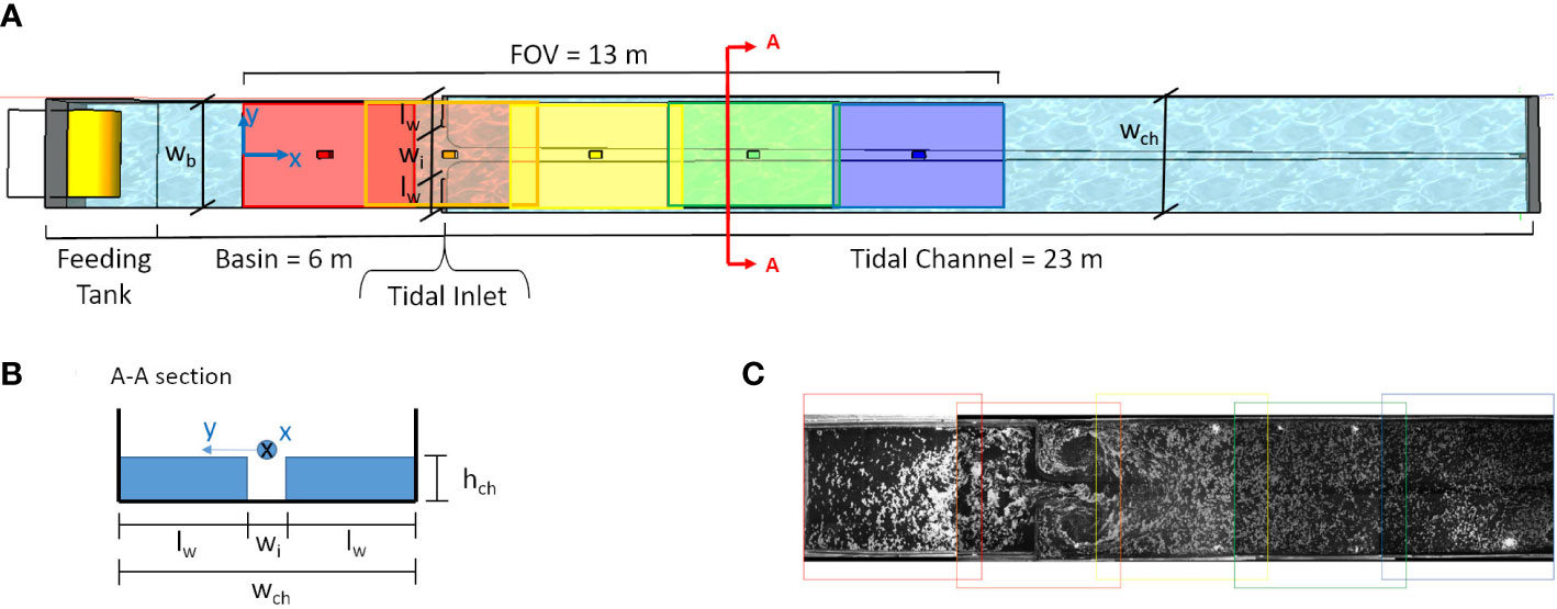
Figure 1 Panel (A) Sketch of the experimental set up and measuring systems. Panel (B) Sketch of channel cross-section. Panel (C) Example of panoramic view after merging process of the five camera acquisitions.

The entire experimental campaign was performed maintaining a constant mean water depth equal to 0.36 m at the channel inlet. The estimate of the conductance coefficient C is about 12, which corresponds to a Manning’s resistance coefficient of about 0.0167 sm^1/3.

In order to reproduce tides, regular volume waves with variable period and amplitude were generated using an oscillating cylinder inside a feeding tank. Wave reflections were minimized by a dissipative sloping mound installed at the end of the channel. A digital signal acquisition-generation system remotely controlled the cylinder. The generated free surface elevation (η) can be described as

$\begin{array}{ll}\eta \left(t\right)={\displaystyle \sum _i{a}_i\text{sin}({\omega }_{i}t+{\varphi }_i)}& (1)\end{array}$

where t is the time, a_i is the amplitude, ϕ_i is the phase shift and ω_i = 2π/T_i the tidal angular frequency of the i^th tidal component, being T_i the tidal period. In the following, we take advantage of this general formulation in order to distinguish between single component tides and multiple components tides.

During a first set of experiments, the tidal channel was forced with a series of single harmonic tides of the kind η(t) =a sin (ωt). In particular, 5 different amplitudes a for 4 tidal periods T [editor]hashave been considered, resulting in a total of 20 experiments.

A second series of experiments, consisting of a total of 19 runs, aimed to mimic more realistic tidal waves using multiple constituents for the tidal forcing signal. A simplified form for the astronomical tidal free surface oscillation has been imposed as:

$\begin{array}{ll}\left(t\right)=a_{sd}\text{sin }({\omega }_{sd}t)+a_d\text{sin}\left(\frac{{\omega }_{sd}}{2}t+\varphi \right)& (2)\end{array}$

where a_sd and a_d represent the amplitude of a semidiurnal and diurnal component respectively, and ω_sd = 2π/T_sd is the angular frequency of the semidiurnal component of period T_sd. For simplicity, we imposed a diurnal period exactly double of the semidiurnal one. The form factor F was used to express the relative importance of semi-diurnal and diurnal components. It is defined as Lee and Chang (2019):

$\begin{array}{ll}F=\frac{a_d}{a_{sd}}& (3)\end{array}$

Specifically, the form parameter can be used to distinguish different astronomical tides: F < 0.25, semi-diurnal tides; 0.25 < F < 1.25, mixed tides, but mainly semi-diurnal; 1.25 < F < 3.0 mixed tides, but mainly diurnal; F > 3.0, the tide is diurnal. To represent real-world scenarios, we varied the form factor F in a range between 0.08 and 1.6 (see Table 1).

TABLE 1

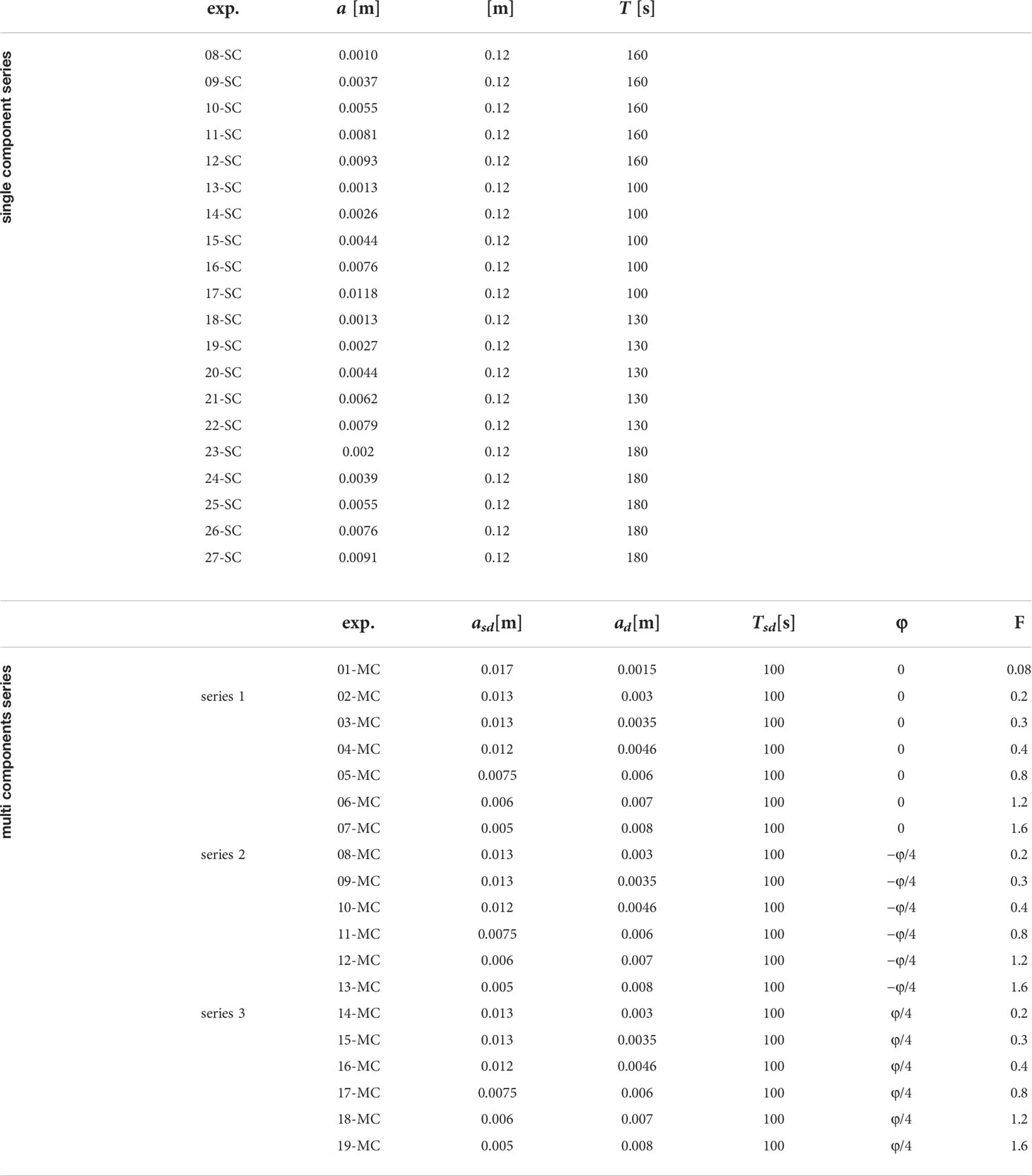
Table 1 Main experimental parameters. SC refers to the single component cases and MC to the multi components series of experiments. For the single component experiments, 7 preliminary runs were performed with the aim to tune the PIV system whereby they are not reported in the table.

In addition, the phase shift ϕ introduced in equation (2) was varied to understand the effect of the phase lag between semi-diurnal and diurnal constituents on the tidal wave shape. In particular, fixing F, we imposed three values of the phase shifts, namely 0, –π/4 and, –π/4.

Large Scale Particle Image Velocimetry (LS-PIV) (Raffel et al., 1998) was employed to measure the two-dimensional time dependent free surface velocity fields u(x,y,t) = [u(x,y,t) v(x,y,t)]. Following the notation of Figure 1A), we denote by x the landward oriented longitudinal axis of the channel with the origin located in the basin at a distance of [editor]34m from the channel inlet and by y the lateral coordinate; u and v are the x and y velocity components, respectively. The large dimension of the area of interest required specific modifications to the equipment respect to the standard PIV technique. Polyethylene particles (940 kg m^-3, mean dimension 3 mm), used as PIV tracers, were distributed uniformly and densely on the channel surface. Lighting was produced using eight 500W white-light halogen lamps. LS-PIV acquisitions were recorded employing five high-resolution GigaEthernet digital camera (Teledyne Dalsa Genie Nano C1280 and C2450). Depending on the camera model, the resolutions varied between 2448×2048 pixels and 1280×1024 pixels. 6-mm lens have been mounted on the cameras. Cameras were fixed on rigid supports at an elevation of 4 m from the bottom of the channel, pointing downwards, yielding a field of view (FoV) that covered a large area of about 13 × 2 m. The FoV extended from about the last 4 m of the basin to about the first 9 m of the channel for the entire width, with cameras overlapping in the longitudinal direction of about 20%. The LS-PIV acquisition frame rate was set equal to 10 fps and, depending on the experimental parameters, each camera recorded between 5000 and 13000 images, for a total of about five tidal periods.

The images from the five digital cameras were then processed in order to obtain a single panoramic image (Figure 1C) of the entire FoV before PIV analysis, performed using the proVision-XS^TM software (Integrated Design Tools Inc). The spatial resolution obtained was about 0.06 m in the x-direction and 0.03 m in the y-direction leading to vector velocity fields evaluated on a grid 211×71.

The present experiments were designed applying rigorous physical scaling laws preserverving the friction parameter as described in Toffolon et al. (2006), χ = ϵL_g/(2πC²D₀), where ϵ = a/D₀ is the dimensionless tidal amplitude, D₀ is the mean water depth, $L_g=T\sqrt{g{D}_0}$ is the inviscid wavelength and C is the Chézy coefficient that represents the ratio between friction and inertia. For details on the scaling arguments and the applicability of the results to realistic contexts we refer to De Leo and Stocchino (2022).

2.2 Lagrangian Coherent Structures background and identification strategy

Here we introduce Lagrangian Coherent Structures (LCS) by means of the Finite-Time Lyapunov Exponents (FTLE). The concept of LCS was first developed by Haller and Yuan (2000) among others, and then further studied by Shadden et al. (2005); Lekien et al. (2005); Haller and Beron-Vera (2012), among many others. The time-dependence of the velocity field inferred by the particle trajectories employed in the Lagrangian approach is more effective in identifying persistent coherent structures than the Eulerian methods, although the Eulerian and the Lagrangian framework share some important links s (Enrile et al., 2020).Moreover, LCS has the advantage that can be directly applied to non-periodic flows, and to flows that are defined by discrete data sets over a finite time interval (Haller, 2002).

Applying the conservation laws of continuum mechanics, we will introduce Finite Lyapunov Exponents. In order to describe the position of a particle ξ of a fluid body B, we define a one-to-one correspondence between the particles and the coordinates of a reference system. The Lagrangian coordinates then read ξ = (ξ¹,ξ²,ξ³) and define a label for fluid particles as a material coordinate system. At this point, it is possible to define a continuous and differentiable transformation ϕ, called flow map, that allows a link between the Lagrangian and the Eulerian coordinate system:

$\begin{array}{ll}x=\Phi \left(t,t_0,\xi \right).& (4)\end{array}$

This transformation can be inverted in a point neighbourhood, provided that Jacobian exists and does not vanish (Aris, 1962). Note that the study of fluid flows cannot be fulfilled disregarding the velocity fields. Indeed, velocity fields are the core of fluid mechanics and time-dependent velocity fields are generally written as v(x,t). The trajectories of particles are curves solutions of

$\begin{array}{ll}\frac{dx}{dt}=u\left(x,t\right)& (5)\end{array}$

with initial conditions x(t₀,ξ) = ξ. With the aim to evaluate the distance that two initial close particles ξ₀ and ξ₀ + ϵ may experience on a finite time interval T = (t₀,t₁), we can apply a linearisation (Allshouse and Peacock, 2015) such as:

$\begin{array}{ll}\delta x=\Phi \left(t_1,t_0,{\xi }_0\right)-\Phi \left(t_1,t_0,{\xi }_0+ϵ\right)\approx \nabla \Phi \left(t_1,t_0,{\xi }_0\right)ϵ& (6)\end{array}$

where ∇Φ(t₁,t₀,ξ₀) is the tensor flow map gradient and it is defined as

$\begin{array}{ll}\nabla {\Phi }_j^i=\partial x_i/\partial {\xi }_j& (7)\end{array}$

We impose that an infinitesimal material element dx must not split along its evolution and coalescence of two material elements does not occur: this is the physical interpretation of the condition on the Jacobian of equation (4).Moreover, the deformation must preserve orientation, that is three right-handed material elements dx, dy and dz satisfying dx ∧ dy dz >0 are transformed into three material elements satisfying

$\begin{array}{ll}\begin{array}{c}dx\wedge dy·dz=\left(\nabla \Phi dx\right)\wedge \left(\nabla \Phi dy\right)·\left(\nabla \Phi d\right)\\ =det\left(\nabla \Phi \right)dx\wedge dy·dz>0.\end{array}& (8)\end{array}$

This second restriction implies that the Jacobian of equation 4 must satisfy:

$\begin{array}{ll}J=det\left(\nabla \Phi \right)>0& (9)\end{array}$

The magnitude of the final distance can be evaluated as (Shadden et al., 2005):

$\begin{array}{ll}\begin{array}{cc}\left|\delta x\left(t_1\right)\right|& =\sqrt{\delta x\left(t_1\right)·\delta x\left(t_1\right)}=\sqrt{\left[\nabla \Phi \delta x\left(t_0\right)\right]·\left[\nabla \Phi \delta ymbolx\right]\left(t_0\right)}\\ & =\sqrt{\delta x\left(t_0\right)·\left[C\delta x\left(t_0\right)\right]}=\sqrt{ϵ·\left(Cϵ\right)}\end{array}& (10)\end{array}$

where C is the Cauchy-Green tensor evaluated as

$\begin{array}{ll}C={(\nabla \text{Φ})}^T\nabla \text{Φ}& (11)\end{array}$

where (•)^T denotes the transpose. It is possible to prove that matrix C is positive definite and symmetric. Since we analyse 2D velocity fields, C has two eigenvectors e₁ and e₂ associated with two eigenvalues0 < λ1 ≤ λ₂, respectively. This means that two main directions can be recognized, tangent to the eigenvectors associated with the maximum and minimum eigenvalues and called unstable and stable directions respectively, and in particular the magnitude of a concentration gradient will decay in time along the unstable direction (Thiffeault and Boozer, 2001). In particular, let us consider for example a saddle point p within an initial tracer distribution D(t₀), with its unstable manifold W^u intersecting the boundary of D(t₀) at a nonzero angle. The material will be transported exponentially fast by the flow map along this unstable manifold, leading to a fingering-type instability (Olascoaga and Haller, 2012). The unstable manifold is thus a stretching line. When δx(t₀) is aligned with the eigenvector associated to the maximum eigenvalue of C, the maximum stretching occurs:

$\begin{array}{ll}\text{max}\left|\delta x\left(t_1\right)\right|={\text{e}}^{{\sigma }_{t_0}^{t_1}\left|\tau \right|}\left|\overline{ϵ}\right|& (12)\end{array}$

where

$\begin{array}{ll}{\sigma }_{t_0}^{t_1}=\frac{1}{\left|\tau \right|}\text{log}\sqrt{{\lambda }_2}=\frac{1}{2\left|\tau \right|}\log {\lambda }_2& (13)\end{array}$

represents the (maximum) Finite-Time Lyapunov Exponent (FTLE) calculated on a finite integration time τ and $\overline{ϵ}$ is the initial perturbation aligned with the eigenvector associated with the maximum eigenvalue of C. Note that a coordinate transformation does not produce any changes in FTLE calculation: for this reason FTLE are considered objective quantities. Computing σ in forward time (t» t₀), repelling manifolds at t₀ are recognized to be the local maxima (i.e. ridges) of the ${\sigma }_{t_0}^{t_1}$ and, similarly, the attracting ones correspond to ridges in the ${\sigma }_{t_0}^{t_1}$ , calculated in backward time (t« t₀).

(Shadden et al., 2005; Haller and Beron-Vera, 2012).describe and quantify the material transport, and forecast large-scale flow features and mixing processes (Haller, 2015). Following the definition of Mathur et al. (2007), a ridge in FTLE field, that behaves as an attractor, is the solution of

$\begin{array}{ll}\frac{d{x}_0}{ds}=\nabla {\sigma }_{t_0}^{t_1}\left(x_0\right)& (14)\end{array}$

with s the arclength along the gradient lines. As pointed out by [46], LCS ridges are FTLE’s gradient lines transversal to the minimum curvature direction, across which the flux is usually negligible (even if non zero) and hence they act as transport barriers. Haller (2011) improved the above definition stating that, in order to be recognized as a LCS, two key properties must be respected: FTLE should be a material surface [as already said by Shadden et al. (2005)] and should exhibit locally the strongest attraction, repulsion, and shearing in the flow. This latter aspect is linked with the hyperbolicity criterion: it enables to observe LCS as cores of Lagrangian patterns. In particular, finding the local maxima in FTLE does not identify LCS, indeed it has been found out by Lekien et al. (2005) and Tang et al. (2010) that FTLE in real-data sets could also not attract or repel nearby trajectories. Thus, four condition must hold in order for an FTLE to be a LCS ridges:

● λ₂ of ${\sigma }_{t_0}^{t_1}$ must be larger that one with one-multiplicity, λ₁ ≠ λ₂ > 1;

● FTLE ridge has to be normal to the eigenvector of λ₂, e₂(x₀), field;

● the gradient of λ₂ in directions parallel to e₂(x₀) must be small 〈 ∇λ₂(x₀,t₀,T),e₂(x₀) 〉=0;

● FTLE must be steep, i.e. the Hessian of the Cauchy-Green tensor evaluated on the strongest strain eigenvector field is positive, ∇²C⁻¹(x₀)>0.

2.3 Lagrangian-averaged vorticity deviation (LAVD)

A peculiar type of LCS are Elliptic LCS, closed and nested material surfaces that act as building blocks of the Lagrangian equivalents of vortices, i.e., rotation-dominated regions of trajectories that generally traverse the domain without substantial stretching or folding. Geodesic vortex detection Haller and Beron-Vera (2012) seeks time t₀ positions of Lagrangian vortex boundaries as outermost closed stationary curves of a specific material-line-averaged tangential stretching functional. A computationally easier approach to Elliptic LCSs consists in obtaining a well-defined bulk rotation for each material element by employing the unique left and right polar decompositions of the flow gradient. The former approach (geodesic) ismore stringent than the latter. Both capture the same Lagrangian vortex regions but the former yields tighter vortex boundaries (Hadjighasem et al., 2017).

Polar decomposition is here adopted in order to overcome issues related to non-objectivity and dynamical inconsistency. We refer to Dynamic Polar Decomposition (DPD) in the form (Haller, 2016):

$\begin{array}{ll}\nabla \Phi \left(t_1,t_0,\xi \right)=O\left(t_1,t_0,\xi \right)M\left(t_1,t_0,\xi \right)=N\left(t_1,t_0,\xi \right)O\left(t_1,t_0,\xi \right)& (15)\end{array}$

where the proper orthogonal tensor O is the dynamic rotation tensor and the non-singular tensors M and N are the right dynamic stretch tensor and left dynamic stretch tensor, respectively. Just as the classic polar decomposition, the DPD is valid in any finite dimension. We write the velocity gradient ∇u as

$\begin{array}{ll}\nabla u\left(x,t\right)=D\left(x,t\right)+W\left(x,t\right)& (16)\end{array}$

where D is the rate-of-strain tensor and W is the spin tensor. The proper orthogonal dynamic rotation tensor O=∇_a0a(t) is the deformation gradient of the purely rotational flow

$\begin{array}{ll}\dot{a}=Wa& (17)\end{array}$

and the non-degenerate right dynamic stretch tensor M=∇_b0b(t) is the deformation gradient of the purely straining flow

$\begin{array}{ll}\dot{b}=O\left(t_0,t_1,\xi \right)DO\left(t_1,t_0,\xi \right)b& (18)\end{array}$

The dynamic rotation tensor O can further be factorized into two deformation gradients related to rigid-body rotation and to deviations from uniform rotation, respectively. As a result

$\begin{array}{ll}O\left(t_1,t_0,\xi \right)=\Omega \left(t_1,t_0,\xi \right)\zeta \left(t_1,t_0,\xi \right)& (19)\end{array}$

where the proper orthogonal relative rotation tensor Ω(t₁,t₀,ξ)=∇_α0α(t) serves as the deformation gradient of the relative rotation flow

$\begin{array}{ll}\dot{a}=\left(W-\overline{W}\right)\alpha & (20)\end{array}$

where$\overline{·}$ denotes a spatial mean over a time-dependent spatial domain. On the contrary, the proper orthogonal mean-rotation tensor ζ=∇_β0β is the deformation gradient of the mean-rotation flow

$\begin{array}{ll}\dot{\beta }=\Omega \left(t_0,t_1,\xi \right)\overline{W}\Omega \left(t_1,t_0,\xi \right)\beta .& (21)\end{array}$

Ω(t₁,t₀,ξ) is dynamically consistent and the total angle swept by this tensor around its own axis of rotation ψ(t₁,t₀,x₀) satisfies

$\begin{array}{ll}\psi \left(t_1,t_0,x_0\right)=\psi \left(t_1,s,x_0\right)+\psi \left(s,t_0,x_0\right)& (22)\end{array}$

The intrinsic rotation angle ψ(t₁,t₀,x₀) is also objective, and is equal to half of the Lagrangian-averaged vorticity deviation (LAVD) defined as (Haller et al., 2016)

$\begin{array}{ll}\text{LAVD}\left(t_1,t_0,x_0\right)={\displaystyle {\int }_{t_0}^{t_1}\left|\omega \left(x\left(s,x_0\right),s\right)-\overline{\omega }\right|}ds,& (23)\end{array}$

where ω is the local vorticity and $\overline{\omega }$ is the spatial mean of vorticity defined as

$\begin{array}{ll}\overline{\omega }=\frac{{\displaystyle {\int }_{U\left(t\right)}\omega \left(x,t\right)dV}}{vol\left(U\left(t\right)\right)}& (24)\end{array}$

U(t) is the time-dependent spatial domain and vol(·) denotes the volume for three-dimensional flows or the area for two dimensional flows.

3 Results

This Section is devoted to present the result of the research. The main focus is related to the Lagrangian interpretation of the dynamics of the flow according to the theoretical background introduced in Section 2.2.

Firstly, the general flow pattern is presented through FTLE maps. This representation gains major insights by looking specifically at lobe dynamics, shear structures and the classical attracting and repelling barriers. Subsequently, vortex interaction is studied directly by applying LAVD.

3.1 The periodical flows around the tidal inlet

Firstly, a general study of FTLE distribution is carried out in agreement with Huhn et al. (2012) and Tang and Boozer (1996). Figure 2 shows the probability distribution function of FTLE fields. At the increasing of τ, pdfs tend to narrow. Similarly, mean, standard deviation and skewness tend to decrease, as shown on Panels b) and c). For large times the pdf converges to its asymptotic form (Abraham and Bowen, 2002; Huhn et al., 2012), which in the case of a delta function denotes a uniform FTLE field without any spatial information and a vanishing variance. This limit in the present case is only hypothetical. However, pdfs behave as expected by the theory. Meaningful LCSs can thus be obtained adopting a value of τ for which pdf’s mean and standard deviation start to superimpose one over each other. In correspondence of approximately 100 s these quantities start to converge: there exists a change in the slope of these curves, pointing out the characteristic integration time that allows for the emerging of the most prominent LCSs (Enrile et al., 2018b).

FIGURE 2

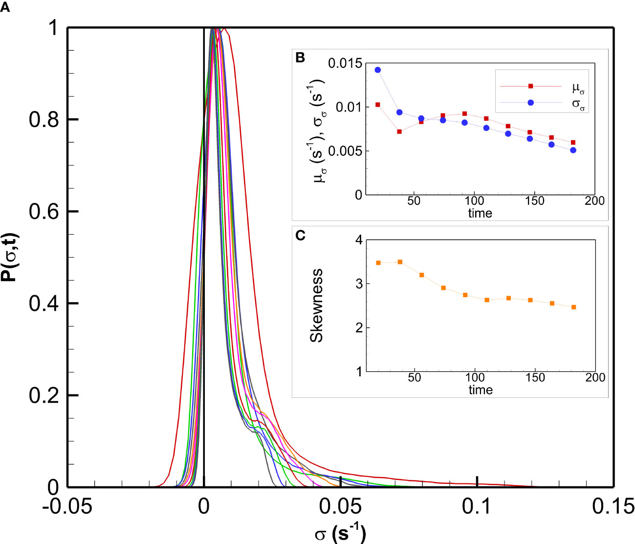
Figure 2 Experiment 24. Panel (A) The probability distribution of the Finite-Time Lyapunov Exponents. Panel (B) Mean value µσ and standard deviation σσ of FTLE as function of the integration time. Panel (C) skewness parameter of the probability distribution as function of the integration time.

Figures 3A–D), show forward FTLE computed for increasing tidal period T, i.e. for experiments 24-SC, 09-SC, 19-SC and 14-SC. The integration time τ is kept constant and equal to 100 s. It is worth noting the general features that characterize the flow: the generation of two opposite vortices on the tidal floodplains behind the walls, the presence of quasi-rectilinear structures along the tidal channel which appear approximately at the inlet and a barrier that surrounds the inlet in the tidal bay. In the Supplementary material, a movie showing the evolution of the Eulerian flow fields of experiment 24SC has been provided. The generation of the flood macrovortices is clearly visible as well as their disruption during the ebb phase. In analogy, Figure 4 shows the previous features on backward calculations. The quasi-rectilinear structures along the inlet and the barriers enclosing part of the tidal bay are still present. The vortices are represented as two opposite mushroom-shaped structures (Peng and Dabiri, 2009) on the floodplains that periodically appear and fade out, depending on the flow direction. Both Figures 3, 4 show the increasing of structure-length from Panel a) to Panel d), i.e. at the decreasing of the tidal period, at the maximum flood phase (in Supplementary material, the ebb phase is provided). This justifies the greater flux through the inlet at the decreasing of T with an enhanced entrainment. In particular, for a fixed value of the tidal amplitude, if the period decreases, an increasing velocity intensity occurs. Experiments 24-SC, 09-SC, 19-SC and 14-SC have a tidal period equal to 180 s, 160 s, 130 s and 100 s, respectively. When the integration time τ tends to equal the tidal period T, the interpretation of FTLE fields is harder since particles tend to complete a tidal cycle in the integration time-interval. This results in a break-up of symmetry since, in a tidal cycle, vortices in the floodplains are generated and fade similarly to the barriers that arise in the tidal bay.

FIGURE 3

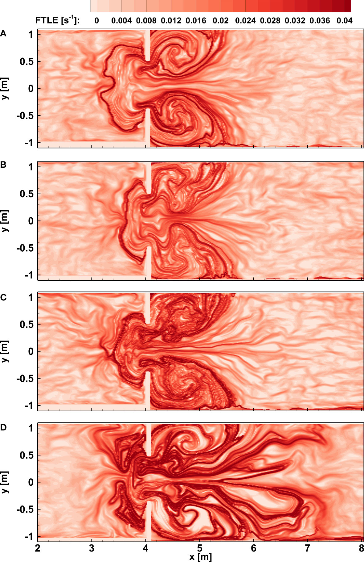
Figure 3 FTLE fields in forward integration of the maximum flood phase. Results are shown maintaining the amplitude of the tide and changing the tidal period. Experiments panel (A) 24, (B) 09, (C) 19 and (D) 14.

FIGURE 4

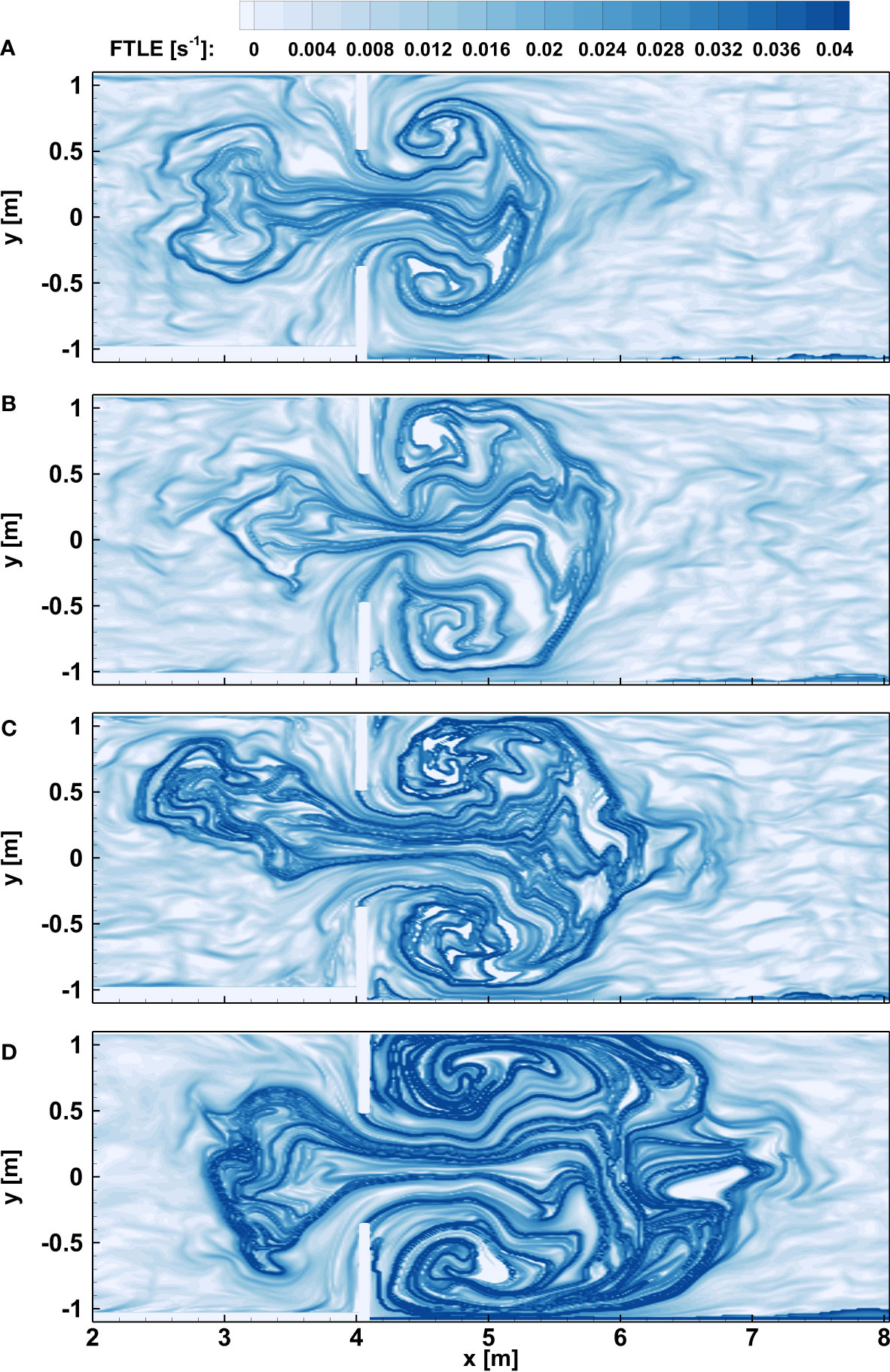
Figure 4 FTLE fields in backward integration of the maximum flood phase. Results are shown maintaining the amplitude of the tide and changing the tidal period. Experiments panel (A) 24, (B) 09, (C) 19 and (D) 14.

Superposition of forward and backward structures is fundamental in order to understand the mutual interaction. Figure 5 shows LCSs of experiment 24-SC calculated in agreement with Mathur et al. (2007). The peculiar presence of superimposed forward and backward structures guaranties leads to the birth of shear LCSs (Beron-Vera et al., 2010; Enrile et al., 2018a; Enrile et al., 2018b).

FIGURE 5

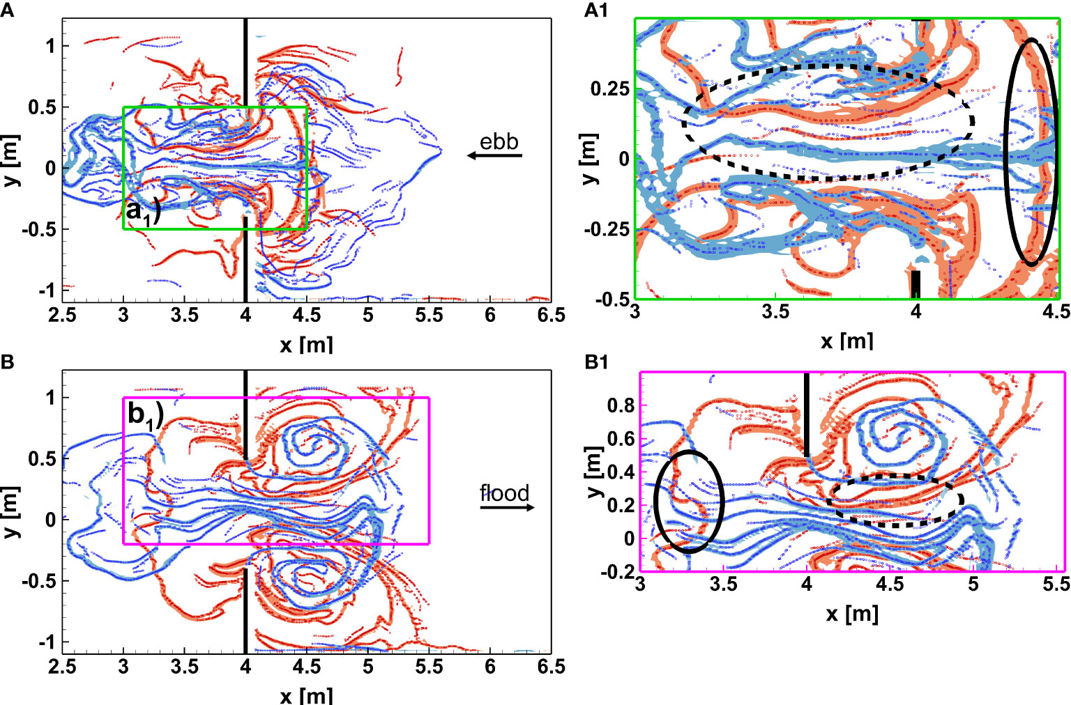
Figure 5 Ridges in superposition of forward (red) and backward (blue) integration of FTLE field: Experiment 24. Panel (A) ebb phase; panel a1) focus of shear (dashed oval) and barrier (solid oval) structures. Panel (B) flood phase; panel b1) focus of shear (dashed oval) and barrier (solid oval) structures.

Shear and Shearless LCSs have a peculiar behavior among the LCS family. The former maximizes shear whereas the latter marks absence of it. Shearless LCSs can be identified as trenches, i.e. minima, of FTLE fields that superimpose on forward and backward computations. For example, Enrile et al. (2018a) and Beron-Vera et al. (2010) identify shearless LCSs in this manner. On the contrary, shear LCSs can be detected as forward and backward ridges of FTLE fields that superimpose one over each other. Enrile et al. (2018a) find both shear and shearless structures following this approach. Sanderson (2014) finds shearing material lines, such as the boundaries of a riverbed in a 3D model of the New River Inlet, Onslow, North Carolina

Figures 5A, B show ebb and flood phases, respectively. The zoomed regions in Panels a₁) and b₁) magnify the inlet where quasi-rectilinear structures are superimposed. A shear dominated area arises where normal attraction and repulsion are no more the key features of the flow. Ridges of forward and backward FTLE fields superimposed one over each other are here identified. Interpretation of FTLE ridges here should be careful since the usual pattern consisting in attracting and repelling barriers could be enriched by shear structures. Indeed, particle paths are normal to the entrance and aligned with LCSs. Dashed ovals in A1, B1 show shear LCSs whereas solid ovals identifies typical attracting and repelling structures, which tend to intersect at right angles. Forward structures tend to mark barriers beyond which particle advection is inhibited. On the contrary, backward structures show lines of accumulation, where mass transfer is enhanced. Forward structures tend to mark separation lines along which particles are repelled to each other. On the contrary, backward structures show lines of accumulation, along which particles tend to be collected, without transfer of mass. Attracting structures mark preferential lines along which transport is likely to develop. It worth noting that changing the tidal period the size of the structures increase, as already pointed out. However, the particle-accumulation areas and the barrier behaviors are consistent for all experiments taken into account.

3.2 Vortex dynamics

Vortex dynamics is usually carried out from an Eulerian reference of frame (Okubo, 1970; Hua and Kline, 1998; Liu et al., 2018; Adrian et al., 2000). However, the Lagrangian point of view allows for a deeper insight in terms of mass transport. A very interesting approach relies on the use of Lagrangian Averaged Vorticity Deviation. LAVD is computed over a finite-time interval and its evolution should be studied upon such a time frame by the advection of closed contours of LAVD fields. However, a FTLE-like approach is here devised in order to highlight vortex shedding from solid edges, evolution and eventual fading of vortex formations. Figure 6 shows subsequent LAVD fields from flood [(Panels a) to d)] to ebb [(Panels e) to f)]. The several time-instances are reported on the top Panel where the plot velocity vs. time is depicted in non-dimensional form. In particular, in Panel 1) the time evolution of the normalized velocity is shown within the point marked in blue in Panel a). The red dots in Panel 1) depict the different Panels in Figure 6. The detachment of the boundary layer at the solid edge of the inlet is very well captured in Panels a) and b). The vortex shedding appears well marked in Panel c), whereas in Panel d) only the core vortices appear, with no vortex shedding phenomenon highlighted. Panels e) and f) show the destruction of the two counter-rotating vortices due to the ebb phase. This approach shows LAVD fields calculated over different, even if adjacent, time intervals, thus not belonging to the same time-domain. Despite being formally not consistent with a rigorous dynamical approach (Farazmand and Haller, 2013), this approach is straightforward in highlighting vortex formation, interaction and fading and the possible error is negligible thanks to the controlled laboratory conditions.

FIGURE 6

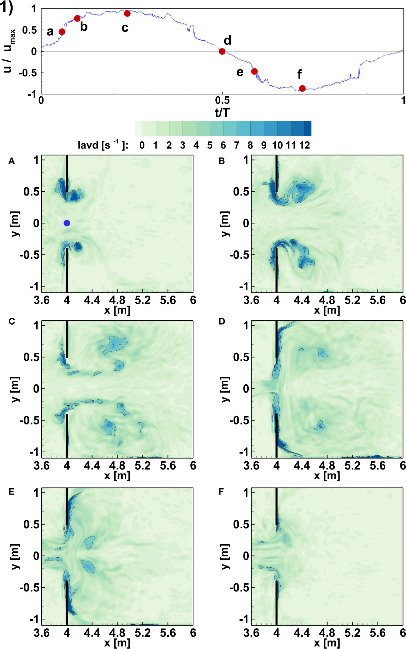
Figure 6 Panel 1) Non dimensional horizontal velocity u/umax as a function of the ratio between time and tidal period. The time signal is extracted at a coordinate x = 4 m and y = 0 m, marked by a blue dot in panel (A). Red dots correspond to panel names below. Panels (A–F) Contours of LAVD at different times. In particular panels (A–D) correspond to flood phase and panels (E, F) to ebb phase. Note that domain reported is restricted to the region around the inlet. Data from experiment 24.

A particular insight on vortex interaction is presented in Figure 7A, B show a dynamically consistent approach where LAVD contours and LAVD fields are advected on the time-interval of calculation. The integration time here is chosen to be equal to 15 s, which is characteristic period of the emission of vortices from the solid boundaries. Vortices are born from the solid edge and advected to the floodplains where they interact, tend to group and finally coalesce.

FIGURE 7

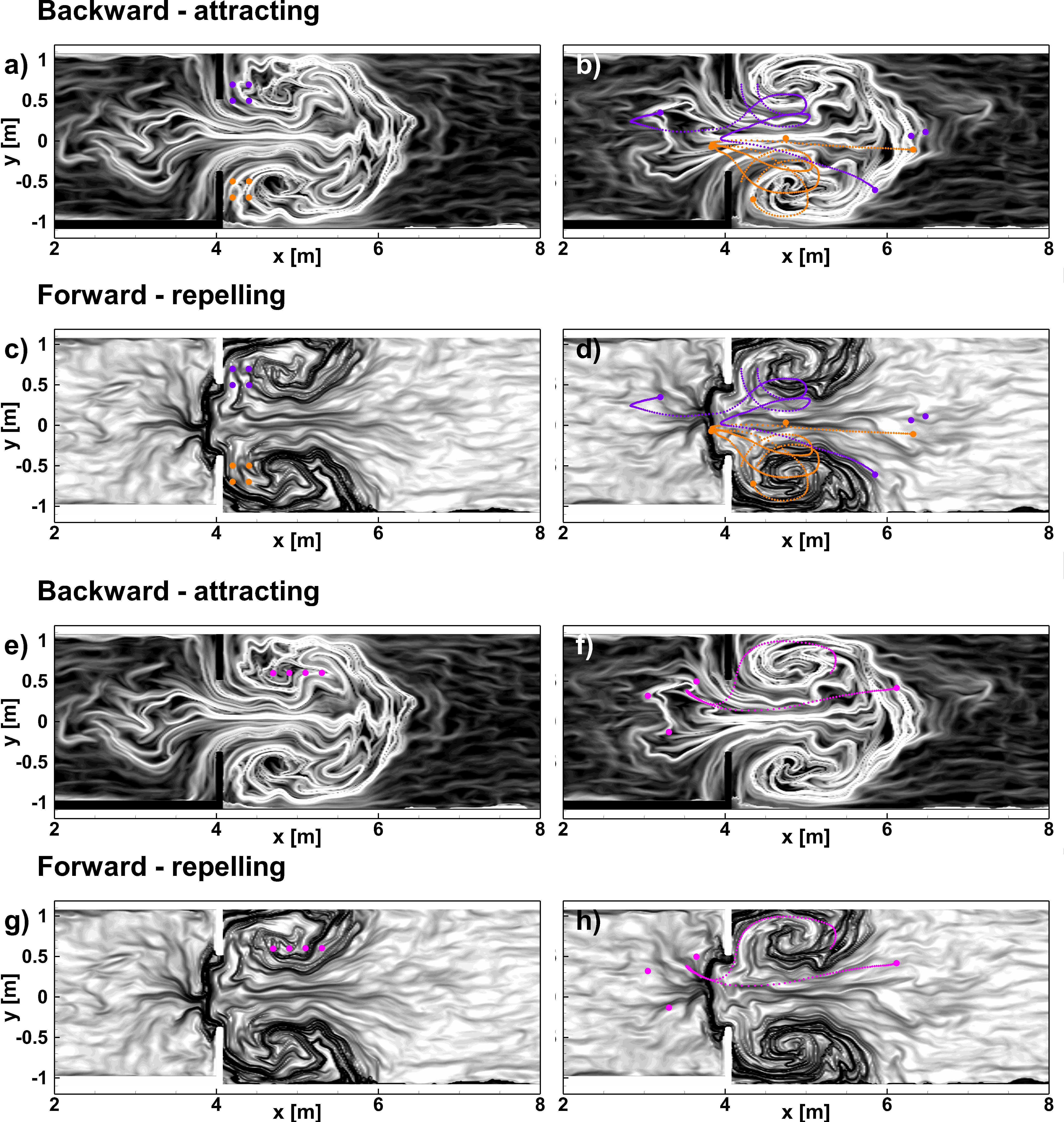
Figure 7 Panel (A) initial time of particle releasing 1 on backward FTLE field; panel (B) final time. Panel (C) initial time of particle releasing 1 on forward FTLE field; panel (D) final time. Panel (E) initial time of particle releasing 2 on backward FTLE field; panel (F) final time. Panel (G) initial time of particle releasing 2 on forward FTLE field; panel (H) final time.

A quantity commonly employed for describing the vortex shedding mechanism is the Strouhal number, defined as:

$\begin{array}{ll}{S}_t=\frac{fL}{U}& (25)\end{array}$

where f is the typical frequency of vortex shedding, L and U are typical length and velocity scale, respectively. However, in previous studies on tidal flows the frequency f has been introduced as the inverse of the dominant tidal period d (Wells and van Heijst, 2003; Nicolau del Roure et al., 2009; Vouriot et al., 2019). In the present case, the length scale is the inlet barrier dimension l_i andthe velocity scale is the peak velocity at the inlet. Using the values for the different experiments, the Strouhal number ranges between 0.05 and 0.2, which implies an emission of about 10 vortices per tidal period. Thus, the integration time for the LAVD was chosen accordingly.

A similar phenomenon was already captured by Haller et al. (2016), however on satellite measures. Here, PIV instrumentation is employed in order to detect LCSs and vortices on a laboratory scale. It is worth mentioning that the LAVD field is also advected with the vortices showing a strong coherence demonstrated by the preservation of rotational coherence inside the material boundaries of the vortices. Panel b) of Figure 7 shows a strong filamentation, too. This filamentation is due to major tangential velocity that stretch the vortex boundary without a global breakaway of material.

4 Discussion

A comprehensive study of vortex shedding and interaction is here carried out from a laboratory experimental campaign. The interplay between a tidal flow and a barrier island inlet is studied applying Lagrangian Coherent Structures (LCSs). In particular, the research adopted a heuristic diagnostic, i.e. Finite-Time Lyapunov Exponent (FTLE), and Lagrangian-Averaged Vorticity Deviation (LAVD). LAVD is employed in order to study vortex detachment from the solid boundaries of the tidal inlet and their subsequent interaction.

An extensive literature is available where FTLEs and LCSs are applied to geophysical flows (Lekien et al., 2005; Haller, 2015): their ability to characterize the main features of the flow is indeed guaranteed has been several time proved in the literature and a significant degree of confidence relies on LCSs nowadays. Forward and backward structures in Figures 3, 4, respectively, are able to recognize repelling, attracting, shear and vortex LCSs. The peculiarity of this flow consists in the generation, growth and eventual dissipation of all these features in a periodic manner. (Lekien et al., 2005; Haller, 2015): studied the dipole formation caused by the interaction of a tidal flow in a physical model. In particular, they studied two bays connected by a narrow channel arguing that when fluid flows out of the inlet, the no-slip condition leads to the growth of viscous boundary layers, which contain strong vorticity compared to the ambient fluid. At the sharp corner, the flow separates and the detached sheet of strong vorticity curls in order to create a vortex. Two such vortices are created at the opposite sides of the channel mouth, which may couple together and form a dipole. The present laboratory settings differs from the one of [56] since the tidal mouth links a bay with a compound channel and moreover the connection between the two is made by a thin wall (recalling a barrier island geometry) instead of a finite length channel. In riverine compound channels, LCSs are generated by a shear instability mechanism (Soldini et al., 2004; 357 van Prooijen and Uijttewaal, 2002; van Prooijen et al., 2005; Enrile et al., 2018a) at the transition from the main channel to the floodplains and it is maintained by the river slope. Here, LCSs are generated by the tidal flow which interacts with the inlet mouth. In this geophysical application, a 2D vortex dipole is generated owing to a mechanism which heuristically conforms to the 3D formation of vortex rings. Krieg and Mohseni (2021) 361 studied vortex rings formation through a nozzle in which the 3D vortex is generated by a jet that carries a shear tube which extends in the ambient fluid. At a critical velocity, the shear tube becomes unstable and the vortex ring drives the shear layer to the axis of symmetry. As a result, the shear layer breaks and a complete pinch-off of the vortex ring is obtained. This representation of vortex rings generation is axisymmetric and a 2D section of this 3D phenomenon well represents the application in this research. In Panel a) of Figure 7 four small scales vortices can be recognized and in Panel b) the high LAVD signal (associated to strong vorticity) shows the path followed by the detached vortices. This path is associated with shear instability due to a meandering pattern characteristic of a complete vortex pinch-off. This analogy is cast in order to introduce a physical mechanism of vortex formation in geophysical contexts. The description carried out by Wells and van Heijst (2004); Nicolau del Roure et al. (2009) must therefore be enhanced by the presence of shear LCSs here detected. Their instability determines the migration of the vortices in the floodplains. These vortices then tend to occupy the total depth of the channel generating vortex macro structures that persist until the ebb phase. In our experiments, none of the vortices generated during the flood phase endure in the channel and they are always flushed away at the inversion of the tide.

At the inversion of the flow from ebb to flood phase, the shear LCSs are generated in the channel and during the flood phase vortices are emitted from the corners of the solid boundaries. These vortices propagate towards the floodplains and eventually fade with the subsequent inversion of the flow (from flood to ebb). Attracting and repelling structures can be detected as the main boundaries for particles moving around the inlet domain. Mixing and advection is enhanced inside the boundaries of these LCS.

Figure 8 shows particle paths and FTLEs together. Backward manifolds (Figure 8A, B, E, F) detect attracting structures along which particles tend to accumulate, whereas the forward manifolds (Figure 8C, D, G, H) correspond to flow barriers. In particular, the left column shows the initial position of a set of particles in two different configurations (A, C, E, G) superimposed to the FTLE fields in backward (white lines on black background) and forward (black lines on white background) integration. Their evolution in time after a single tidal period is then shown on the right hand column (B, D, F H). Note that the complete trajectory has been highlighted just for a couple of particles for clarity sake. The time evolution of the two deployments over an entire tidal cycle can be found in the movies in the Supplementary Material. Inspecting carefully, particles tend to align with attracting structures and being repelled by the repelling ones, but the real mechanism is indeed more complicate. The boundary which repelling LCSs form is well characterized in panels D, H) where the particles cannot cross the LCS that enclose the inlet. On the contrary, panels B, F show the accumulation of particles on attracting LCS. The transition from the channel (right part) to the tidal bay (left part) occurs along the shear LCSs which are generated along the inlet. In Figure 5, the superposition between forward and backward FTLE fields is shown. Regions in which the two manifolds appear aligned highlight shear structures whereas the intersection between the two recognize saddle point and thus transport barrier (Mathur et al., 2007). Note that this pattern of LCS is repeatedly generated and destructed at every tidal period. The concurrent presence of shear and barriers determine that particles may be trapped between different manifolds, driving them far from each other ending up in different parts of the domain. This pattern is represented through a sketch. Figure 9 shows forward and backward structures in red and blue, respectively. Their intersection is labeled as a time-dependent saddle point. This representation aims to summarize the mutual interaction between repelling and attraction structures and the presence of shear in the inlet. The external borders of these structures tend to expand and shrink in size alternatively in time in agreement with the tidal signal.

FIGURE 8

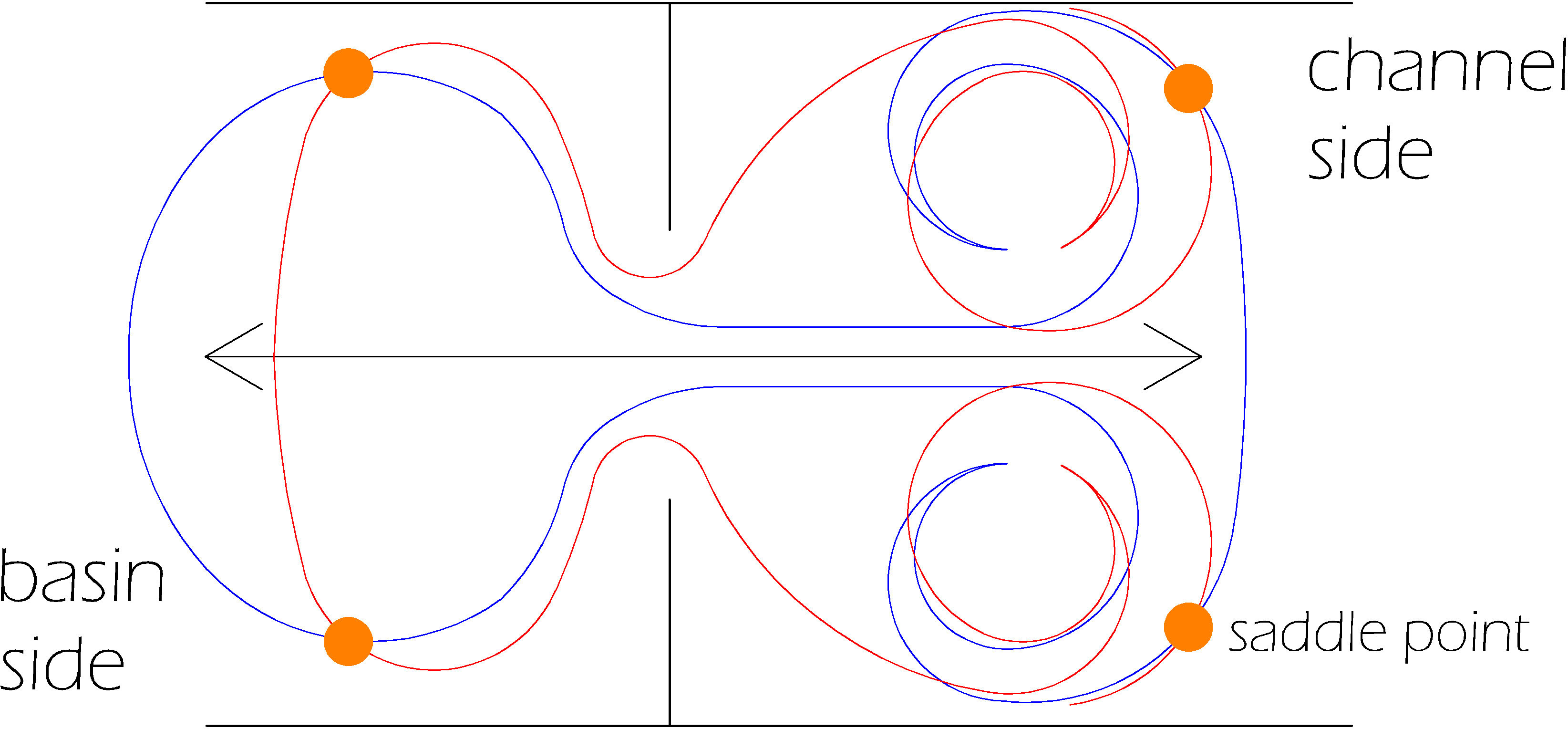
Figure 8 Sketch of forward and backward structures in red and blue, respectively. Their concurrent presence in the inlet generates shear LCSs. Their length and size tend to increase and shrink recursively in time in agreement with the tidal signal.

FIGURE 9

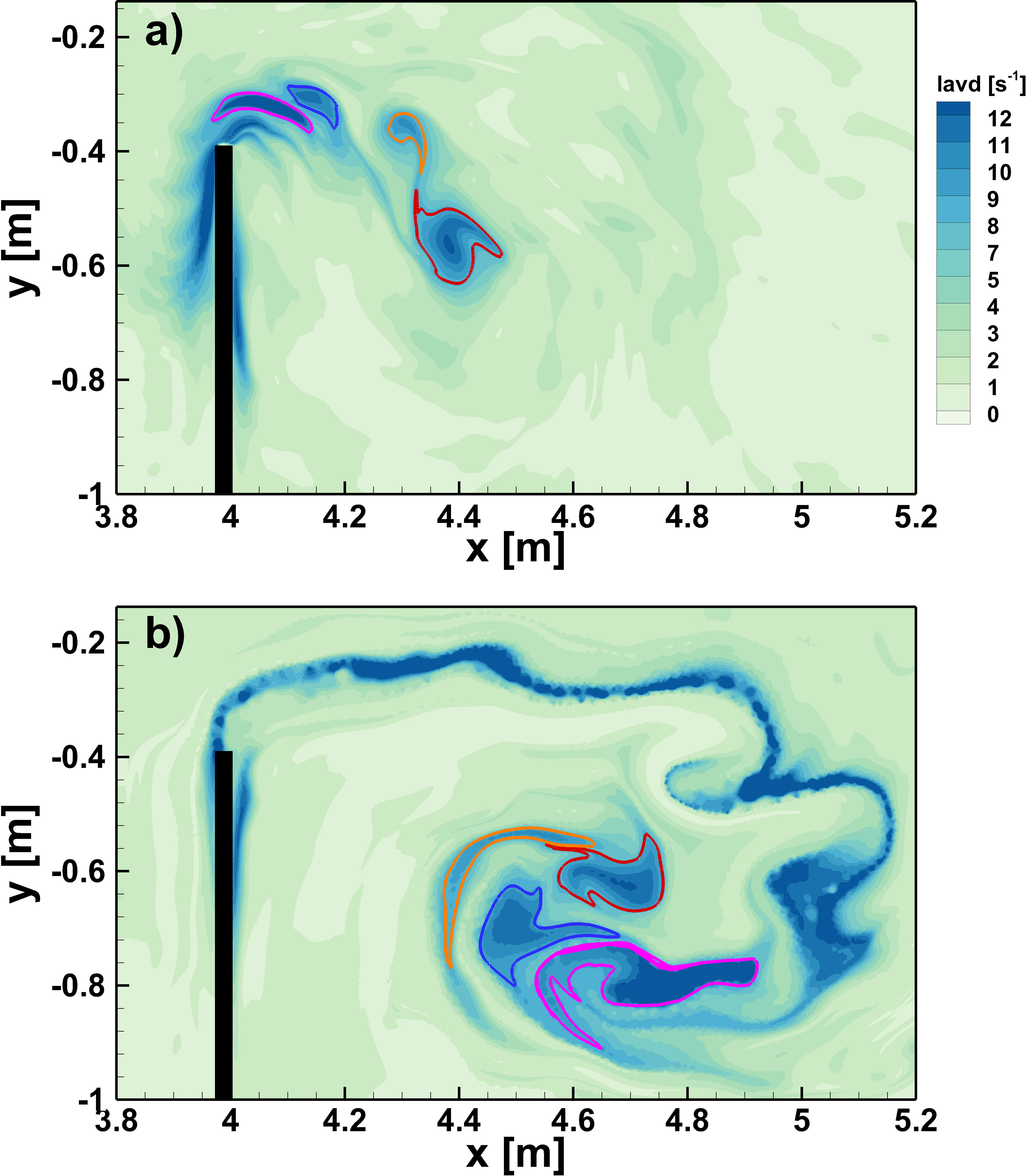
Figure 9 Vortex interaction identified through LAVD. Panel (A) shows LAVD computed in flood phase with vortices identified with closed contour. Panel (B) shows advection of LAVD alongside with the particles that constitute the vortex boundary. Typical filamentation in vortex advection is visible. However, vorticity coherence is maintained inside vortex boundaries. A trail of strong vorticity is depicted in Panel (B), too. Detachment of boundary layer with vortex formation is clearly visible together with the most probable path followed.

Multi component tides were considered in the experimental campaign. Figures of the FTLE fields in forward and backward integration are reported in the Supplementary Materials. From the synthetic signals, see Figure S3, it is possible to appreciate three different compositions of the two tidal components (exp05MC, exp11MC and exp17MC), that result in different flood and ebb tidal excursions. From the FTLE fields it is possible to see that the intrusion of the LCS is larger after most intense flood phases, disregarding the water level reached. The same effect occurs in the ebb cases, not shown for sake of brevity. However, the features underlined by the multi-component experiments do not differ as far as the LCSs pattern is concerned. It is possible that different experimental conditions could lead to a series of multiple jets in the flood phase. For example, spring and neap tides could generate a flow pattern richer in features and structures. Such experimental conditions could be pursued in another experimental campaign.

(Lekien et al., 2005; Beron-Vera et al., 2008; Gough et al., 2016).

Moreover, the different dynamical characteristics of the flow domain, strain or vorticity dominated, are linked to the energy and enstrophy fluxes as observed in De Leo and Stocchino (2022). Indeed, the major outcome of the study was the transitional character of the energy/enstrophy cascades during a single tidal period and this aspect was linked to the presence of vorticity or strain dominated flow structures, in accordance with previous studies (Chen et al., 2003; Chen et al., 2006).

5 Conclusion

Generation, accretion and fading of coherent structures and vortices in fluid flows have always been a very lively scientific research topic (Hussain, 1983; Ottino, 1989; Colagrossi et al., 2021). Since Okubo (1970), researchers laid much of their efforts in detecting vortices applying Eulerian approaches. However, a Lagrangian approach (Haller, 2015) is the most viable way of visualizing coherent structures in unsteady flows. The Lagrangian-approach strength stems out from its foundations: the analysis of particles paths.

This research focuses on a laboratory-scale tidal flow generated through the periodic oscillation of the water level, mimicking tidal waves, across a barrier island inlet that links a bay and a tidal compound channel. Among the multiple Lagrangian diagnostics at our disposal (Hadjighasem et al., 2017), the finite-time Lyapunov exponent (FTLE) (Shadden et al., 2005) and the Lagrangian averaged vorticity deviation (LAVD) are here adopted. The former is chosen thanks to its very versatile characteristics: repelling, attracting and shear structures can be easily detected in forward and backward integrations. The latter presents an intrinsic ability to define vortex boundaries (Haller et al., 2016).

FTLEs here manage to detect a wealth of structures, as depicted in Figures 3, 4, whom most struggling ones are shear structures at the inlet and mushroom-like structures on the floodplains of compound channel behind the walls. Structures calculated in forward and backward time that mainly superimpose one over each other are shear structures. This case occurs at the inlet where quasi-linear barriers are detected at the center of the main channel. Tidal currents that periodically flow through the inlet generate these structures. The detachment of boundary layer from the solid edge of the walls and the concurrent instability of the shear structures which protrude toward the compound channel determine the complete occurrence of two symmetric vortices on both floodplains.

LAVD manages to capture vortex interactions on the floodplains as shown in Figure 7. Their mutual interaction is depicted as vortices are advected in forward time. Moreover, high-LAVD signal meanders as it outdistances the inlet walls. This behavior is a consequence of the shear LCS instability mechanism (Krieg and Mohseni, 2021). Previous studies characterized the behavior of tidal vortices (Wells and van Heijst, 2004), even if in a slightly different geometry. However, this is the first time that shear structures and LAVD are computed from a laboratory experiment on a tidal flow, at least at the author’s knowledge. This work manages to clarify the role played by LCSs in the generation of these tidal vortices, enhancing the scientific knowledge on the subject. In addition, the general behavior of numerical particle paths is studied, both in the tidal bay and in the compound channel. FTLE ridges influence the crossing of the inlet by the particles and define the maximum distance particles can travel on both areas by assessing the extension of attracting LCSs evaluated as backward FTLE ridges.

The analysis described in the present study shed light on the complex interaction of tidal current and geometrical features (e.g. tidal inlet) very often present in natural estuarine and coastal environments. The generation of LCSs might play a fundamental role in the exchange of water masses between the open sea and the tidal channels, possibly increasing the residence time of mass parcels (water, nutrients and pollutants) around the tidal inlet by creating dynamical separations in the flow domain. Thus, this study could have a direct impact on real-world applications related to water quality and sediment transport. As seen in different contributions LCSs are recognized to be useful tools in the recognition of transport barrier r (Lekien et al., 2005; Beron-Vera et al., 2008; Gough et al., 2016). Mixing could be enhanced or prevented by the presence of these structures and vortices. Concentration of pollutant could therefore vary depending on their presence. In addition, sediment transport at the bottom could be altered with possible localized erosion or accumulation areas nearby the inlet.

Data availability statement

The datasets presented in this study can be found in online repositories. The names of the repository/repositories and accession number(s) can be found below: http://10.5281/zenodo.6598687.

Author contributions

AL: conceptualization, experimental activities, data processing and writing. FE: data processing and writing. AS: conceptualization, data processing and writing. All authors contributed to the article and approved the submitted version.

Conflict of interest

The authors declare that the research was conducted in the absence of any commercial or financial relationships that could be construed as a potential conflict of interest.

Publisher’s note

All claims expressed in this article are solely those of the authors and do not necessarily represent those of their affiliated organizations, or those of the publisher, the editors and the reviewers. Any product that may be evaluated in this article, or claim that may be made by its manufacturer, is not guaranteed or endorsed by the publisher.

Supplementary material

The Supplementary Material for this article can be found online at: https://www.frontiersin.org/articles/10.3389/fmars.2022.959304/full#supplementary-material

References

Abraham E. R., Bowen M. M. (2002). Chaotic stirring by a mesoscale surface-ocean flow. Chaos.: Interdiscip. J. Nonlinear. Sci. 12, 373–381. doi: 10.1063/1.1481615

CrossRef Full Text | Google Scholar

Adrian R., Christensen K., Liu Z. (2000). Analysis and interpretation of istantaneous turbulent velocity fields. Exp. Fluid. 29, 275–290. doi: 10.1007/s003489900087

CrossRef Full Text | Google Scholar

Allshouse M. R., Peacock T. (2015). Lagrangian Based methods for coherent structure detection. Chaos.: Interdiscip. J. Nonlinear. Sci. 25, 097617. doi: 10.1063/1.4922968

CrossRef Full Text | Google Scholar

Aris R. (1962). Vectors, tensors and the basic equations of fluid mechanics (New York: Dover Publications INC.).

Google Scholar

Beron-Vera F. J., Olascoaga M. J., Brown M. G., Koçak H., Rypina I. I. (2010). Invariant-tori-like lagrangian coherent structures in geophysical flows. Chaos.: Interdiscip. J. Nonlinear. Sci. 20, 017514. doi: 10.1063/1.3271342

CrossRef Full Text | Google Scholar

Beron-Vera F. J., Olascoaga M. J., Goni G. (2008). Oceanic mesoscale eddies as revealed by lagrangian coherent structures. Geophys. Res. Lett. 35. doi: 10.1029/2008GL033957

PubMed Abstract | CrossRef Full Text | Google Scholar

Cenedese C., Adduce C., Fratantoni D. M. (2005). Laboratory experiments on mesoscale vortices interacting with two islands. J. Geophys. Res.: Ocean. 110. doi: 10.1029/2004JC002734

CrossRef Full Text | Google Scholar

Chen S., Ecke R. E., Eyink G. L., Rivera M., Wan M., Xiao Z. (2006). Physical mechanism of the two-dimensional inverse energy cascade. Phys. Rev. Lett. 96. doi: 10.1103/PhysRevLett.96.084502

CrossRef Full Text | Google Scholar

Chen S., Ecke R. E., Eyink G. L., Wang X., Xiao Z. (2003). Physical mechanism of the two-dimensional enstrophy cascade. Phys. Rev. Lett. 91, 214501. doi: 10.1103/PhysRevLett.91.214501

PubMed Abstract | CrossRef Full Text | Google Scholar

Colagrossi A., Marrone S., Colagrossi P., Le Touzé D. (2021). Da vinci’s observation of turbulence: A french-italian study aiming at numerically reproducing the physics behind one of his drawings, 500 years later. Phys. Fluid. 33, 115122. doi: 10.1063/5.0070984

CrossRef Full Text | Google Scholar

Coulliette C., Lekien F., Paduan J. D., Haller G., Marsden J. E. (2007). Optimal pollution mitigation in monterey bay based on coastal radar data and nonlinear dynamics. Environ. Sci. Technol. 41 (10), 6562–6572. doi: 10.1021/es0630691

PubMed Abstract | CrossRef Full Text | Google Scholar

De Leo A., Stocchino A. (2022). Evidence of transient energy and enstrophy cascades in tidal flows: A scale to scale analysis. Geophys. Res. Lett. 49 (10), e2022GL098043. doi: 10.1029/2022GL098043

CrossRef Full Text | Google Scholar

Enrile F., Besio G., Stocchino A. (2018a). Shear and shearless lagrangian structures in compound channels. Adv. Water Resour. 113, 141–154. doi: 10.1016/j.advwatres.2018.01.006

CrossRef Full Text | Google Scholar

Enrile F., Besio G., Stocchino A. (2020). Eulerian spectrum of finite-time lyapunov exponents in compound channels. Meccanica 55, 1821–1828. doi: 10.1007/s11012-020-01217-y

CrossRef Full Text | Google Scholar

Enrile F., Besio G., Stocchino A., Magaldi M., Mantovani C., Cosoli S., et al. (2018b). Evaluation of surface lagrangian transport barriers in the gulf of trieste. Continent. Shelf. Res. 167, 125–138. doi: 10.1016/j.csr.2018.04.016

CrossRef Full Text | Google Scholar

Farazmand M., Haller G. (2013). Attracting and repelling lagrangian coherent structures from a single computation. Chaos.: Interdiscip. J. Nonlinear. Sci. 23, 023101. doi: 10.1063/1.4800210

CrossRef Full Text | Google Scholar

Gough M. K., Reniers A., Olascoaga M. J., Haus B. K., MacMahan J., Paduan J., et al. (2016). Lagrangian Coherent structures in a coastal upwelling environment. Continent. Shelf. Res. 128, 36–50. doi: 10.1016/j.csr.2016.09.007

CrossRef Full Text | Google Scholar

Hadjighasem A., Farazmand M., Blazevski D., Froyland G., Haller G. (2017). A critical comparison of lagrangian methods for coherent structure detection. Chaos.: Interdiscip. J. Nonlinear. Sci. 27, 053104. doi: 10.1063/1.4982720

CrossRef Full Text | Google Scholar

Haller G. (2002). Lagrangian Coherent structures from approximate velocity data. Phys. Fluid. 14, 1851–1861. doi: 10.1063/1.1477449

CrossRef Full Text | Google Scholar

Haller G. (2011). A variational theory of hyperbolic lagrangian coherent structures. Phys. D.: Nonlinear. Phenomena. 240, 574–598. doi: 10.1016/j.physd.2010.11.010

CrossRef Full Text | Google Scholar

Haller G. (2015). Lagrangian Coherent structures. Annu. Rev. Fluid. Mechanics. 47, 137–162. doi: 10.1146/annurev-fluid-010313-141322

CrossRef Full Text | Google Scholar

Haller G. (2016). Dynamic rotation and stretch tensors from a dynamic polar decomposition. J. Mechanics. Phys. Solid. 86, 70–93. doi: 10.1016/j.jmps.2015.10.002

CrossRef Full Text | Google Scholar

Haller G., Beron-Vera F. J. (2012). Geodesic theory of transport barriers in two-dimensional flows. Phys. D.: Nonlinear. Phenomena. 241, 1680–1702. doi: 10.1016/j.physd.2012.06.012

CrossRef Full Text | Google Scholar

Haller G., Hadjighasem A., Farazmand M., Huhn F. (2016). Defining coherent vortices objectively from the vorticity. J. Fluid. Mechanics. 795, 136–173. doi: 10.1017/jfm.2016.151

CrossRef Full Text | Google Scholar

Haller G., Yuan G. (2000). Lagrangian Coherent structures and mixing in two-dimensional turbulence. Phys. D.: Nonlinear. Phenomena. 147, 352–370. doi: 10.1016/S0167-2789(00)00142-1

CrossRef Full Text | Google Scholar

Hasegawa D., Lewis M., Gangopadhyay A. (2009). How islands cause phytoplankton to bloom in their wakes. Geophys. Res. Lett. 36. doi: 10.1029/2009GL039743

CrossRef Full Text | Google Scholar

Hasegawa D., Yamazaki H., Lueck R., Seuront L. (2004). How islands stir and fertilize the upper ocean. Geophys. Res. Lett. 31. doi: 10.1029/2004GL020143

CrossRef Full Text | Google Scholar

HE C., YIN Z.-Y., Stocchino A., WAI O. W. H., LI S. (2022). The coastal macro-vortices dynamics in hong kong waters and its impact on water quality. Ocean. Model. 175 doi: 10.1016/j.ocemod.2022.102034

CrossRef Full Text | Google Scholar

Hua B. L., Kline P. (1998). An exact criterion for the stirring properties of nearly two-dimensional turbulence. Phys. D. 113, 98–110. doi: 10.1016/S0167-2789(97)00143-7}

CrossRef Full Text | Google Scholar

Huhn F., von Kameke A., Allen-Perkins S., Montero P., Venancio A., Pérez-Muñuzuri V. (2012). Horizontal lagrangian transport in a tidal-driven estuary–transport barriers attached to prominent coastal boundaries. Continent. Shelf. Res. 39-40, 1–13. doi: 10.1016/j.csr.2012.03.005

CrossRef Full Text | Google Scholar

Hussain A. K. M. F. (1983). Coherent structures–reality and myth. Phys. Fluid. 26, 2816–2850. doi: 10.1063/1.864048

CrossRef Full Text | Google Scholar

Krieg M., Mohseni K. (2021). A new kinematic criterion for vortex ring pinch-off. Phys. Fluid. 33, 037120. doi: 10.1063/5.0033719

CrossRef Full Text | Google Scholar

LaCasce J. (2008). Statistics from lagrangian observations. Prog. Oceanog. 77, 129. doi: 10.1016/j.pocean.2008.02.002

CrossRef Full Text | Google Scholar

Lee S.-H., Chang Y.-S. (2019). Classification of the global tidal types based on auto-correlation analysis. Ocean. Sci. J. 54, 279–286. doi: 10.1007/s12601-019-0009-7

CrossRef Full Text | Google Scholar

Lekien F., Coulliette C., Mariano A., Ryan E., Shay L., Haller G., et al. (2005). Pollution release tied to invariant manifolds: A case study for the coast of florida. Phys. D. 210, 1–20. doi: 10.1016/j.physd.2005.06.023

CrossRef Full Text | Google Scholar

Liu C., Gao Y., Tian S., Dong X. (2018). Rortex a new vortex vector definition and vorticity tensor and vector decompositions. Phys. Fluid. 30. doi: 10.1063/1.5023001

CrossRef Full Text | Google Scholar

Mathur M., Haller G., Peacock T., Ruppert-Felsot J. E., Swinney H. L. (2007). Uncovering the lagrangian skeleton of turbulence. Phys. Rev. Lett. 98, 144502. doi: 10.1103/PhysRevLett.98.144502

PubMed Abstract | CrossRef Full Text | Google Scholar

Nicolau del Roure F., Socolofsky S. A., Chang K.-A. (2009). Structure and evolution of tidal starting jet vortices at idealized barotropic inlets. J. Geophys. Res.: Ocean. 114. doi: 10.1029/2008JC004997

CrossRef Full Text | Google Scholar

Okubo A. (1970). Horizontal dispersion of floatable particles in the vicinity of velocity singularities such as convergences. Depp-Sea. Res. 17, 445–454. doi: 10.1016/0011-7471(70)90059-8

CrossRef Full Text | Google Scholar

Olascoaga M. J., Beron-Vera F. J., Haller G., Trinanes J., Iskandarani M., Coelho E., et al. (2013). Drifter motion in the gulf of mexico constrained by altimetric lagrangian coherent structures. Geophys. Res. Lett. 40, 6171–6175. doi: 10.1002/2013GL058624

CrossRef Full Text | Google Scholar

Olascoaga M. J., Haller G. (2012). Forecasting sudden changes in environmental pollution patterns. Proc. Natl. Acad. Sci. 109, 4738–4743. doi: 10.1073/pnas.1118574109

CrossRef Full Text | Google Scholar

Ottino J. M. (1989). The kinematics of mixing: stretching, chaos, and transport ((Cambridge texts in applied mathematics) (Cambridge University Press).

Google Scholar

Peng J., Dabiri J. O. (2009). Transport of inertial particles by lagrangian coherent structures: application to predator–prey interaction in jellyfish feeding. J. Fluid. Mechanics. 623, 75–84. doi: 10.1017/S0022112008005089

CrossRef Full Text | Google Scholar

Raffel M., Willert C. E., Kompenhans J. (1998). Particle image velocimetry: a practical guide Vol. 2 (Berlin: Springer).

Google Scholar

Sanderson A. R. (2014). “An alternative formulation of lyapunov exponents for computing lagrangian coherent structures,” in 2014 IEEE pacific visualization symposium, 277–280. IEEE Computer Society Conference Publishing Services (CPS)

Google Scholar

Shadden S. C., Lekien F., Marsden J. E. (2005). Definition and properties of lagrangian coherent structures from finite-time lyapunov exponents in two-dimensional aperiodic flows. Phys. D.: Nonlinear. Phenomena. 212, 271–304. doi: 10.1016/j.physd.2005.10.007

CrossRef Full Text | Google Scholar

Soldini L., Piattella A., Brocchini M., Mancinelli A., Bernetti R. (2004). Macrovortices-induced horizontal mixing in compound channels. Ocean. Dyn. 54, 333–339. doi: 10.1007/s10236-003-0057-4

CrossRef Full Text | Google Scholar

Tang X. Z., Boozer A. H. (1996). Finite time lyapunov exponent and advection-diffusion equation. Phys. D.: Nonlinear. Phenomena. 95, 283–305. doi: 10.1016/0167-2789(96)00064-4

CrossRef Full Text | Google Scholar

Tang W., Mathur M., Haller G., Hahn D. C., Ruggiero F. H. (2010). Lagrangian Coherent structures near a subtropical jet stream. J. Atmosph. Sci. 67, 2307–2319. doi: 10.1175/2010JAS3176.1

CrossRef Full Text | Google Scholar

Tarshish N., Abernathey R., Zhang C., Dufour C. O., Frenger I., Griffies M. I. (2018). Identifying lagrangian coherent vortices in a mesoscale ocean model. Ocean. Model. 130, 15–28. doi: 10.1016/j.ocemod.2018.07.001

CrossRef Full Text | Google Scholar

Thiffeault J.-L., Boozer A. H. (2001). Geometrical constraints on finite-time lyapunov exponents in two and three dimensions. Chaos.: Interdiscip. J. Nonlinear. Sci. 11, 16–28. doi: 10.1063/1.1342079

CrossRef Full Text | Google Scholar

Toffolon M., Vignoli G., Tubino M. (2006). Relevant parameters and finite amplitude effects in estuarine hydrodynamics. J. Geophys. Res.: Ocean. 111. doi: 10.1029/2005JC003104

CrossRef Full Text | Google Scholar

van Prooijen B., Battjes J., Uijttewaal W. (2005). Momentum exchange in straight uniform compound channel flow. J. Hydr. Engng. 131, 175–183. doi: 10.1061/(ASCE)0733-9429(2005)131:3(175)

CrossRef Full Text | Google Scholar

van Prooijen B., Uijttewaal W. (2002). A linear approach for the evolution of coherent structures in shallow mixing layers. Phys. Fluid. 14, 4105–4114. doi: 10.1063/1.1514660

CrossRef Full Text | Google Scholar

Vouriot C. V., Angeloudis A., Kramer S. C., Piggott M. D. (2019). Fate of large-scale vortices in idealized tidal lagoons. Environ. Fluid. Mechanics. 19, 329–348. doi: 10.1007/s10652-018-9626-4

CrossRef Full Text | Google Scholar

Wells M. G., van Heijst G.-J. F. (2003). A model of tidal flushing of an estuary by dipole formation. Dynam. Atmosph. oceans. 37, 223–244. doi: 10.1016/j.dynatmoce.2003.08.002

CrossRef Full Text | Google Scholar

Wells M., van Heijst G. (2004). “Dipole formation by tidal flow in a channel,” in International symposium on shallow flows. balkema publishers, delft, 63–70.

Google Scholar

Wolanski E., Imberger J., Heron M. L. (1984). Island wakes in shallow coastal waters. J. Geophys. Res.: Ocean. 89, 10553–10569. doi: 10.1029/JC089iC06p10553

CrossRef Full Text | Google Scholar