The essential observations for reconstructing full-depth tidal currents

Based on the modal decomposition and least square method, full-depth tidal currents and corresponding internal tidal modes can be obtained from limited observations. Through a series of experiments based on direct observations at the mooring MP1 and synthetic observations at the moorings MP2 and MP3 in the South China Sea, the essential observations for reconstructing full-depth tidal currents are determined. Both observations in the upper ocean (especially near the thermocline) and deep layer (below 500 m) are essential in the reconstruction. For the upper ocean, an up-looking acoustic Doppler current profiler near the thermocline is generally essential, which can also be replaced by at least 2-4 current meters (CMs). The number of CM depends on the complexity and range of buoyancy frequency variation. For the deep layer, more observations are needed as water depth increases. The observations with the CM interval/water depth ratios about 0.2 can effectively reconstruct full-depth tidal currents below 500 m based on one barotropic mode and first three baroclinic modes. Significantly, the CMs in the middle of the deep layer are more important than those at two ends of the deep layer, which may provide more cost-effective design at a small loss of accuracy. Furthermore, the CMs with the depth interval/water depth ratios less than 1/8 in the deep layer can effectively reconstruct full-depth tidal currents with high-mode baroclinic motions.

1 Introduction

As a ubiquitous motion in the stratified ocean, internal tides (ITs) play an important role in dissipating surface tidal energy (Munk, 1997; Egbert and Ray, 2000) and enhancing ocean mixing (Niwa and Hibiya, 2001; Rudnick et al., 2003; Tian et al., 2009; Li et al., 2021; Wang et al., 2021), and finally contribute to large-scale ocean circulations (Xie et al., 2018., Wang et al., 2019). In regional oceans, ITs are an important intermediate process in the generation of internal solitary waves (Chao et al., 2007), and can interact with near-inertial waves (Guan et al., 2014) and mesoscale eddies (Dunphy and Lamb, 2014). Generated by barotropic tidal currents flowing over varying topographies, intense ITs are always found near mid-ocean ridges, seamounts, continental shelves and slopes, such as the Hawaiian Ridge (Rudnick et al., 2003; Simmons et al., 2004; Zhao et al., 2010) and Luzon Strait (Jan et al., 2007; Alford et al., 2011; Buijsman et al., 2012; Buijsman et al., 2014; Zhao, 2014; Alford et al., 2015).

One important approach to study ITs is to place subsurface moorings and analyze their observations. Through analyzing observations from acoustic Doppler current profilers (ADCPs), current meters (CMs), CTDs and thermometers, characteristics of ITs, such as coherence, incoherence, modal structure, energy flux and seasonal variability, have been studied by many scholars (Zhao et al., 2010; Alford et al., 2011; Guo et al., 2012; Xu et al., 2013; Cao et al., 2015; Shang et al., 2015). Among these characteristics, the modal structure and energy flux are of great importance, representing the vertical structure and propagation of internal tidal energy. However, analysis on the modal structure and energy flux requires full-depth observations in principle. Great challenges still remain for the acquisition of full-depth observations in the deep ocean due to water depth and limitations of measuring instruments. Katsumata et al. (2010) used vertical interpolation and extrapolation of the moored point measurements to know velocity and pressure throughout the water column. However, purely mathematical interpolation tools such as linear, polynomial, or spline functions, which could be used for interpolation/extrapolation, usually lack physical explanations. Fortunately, recent studies indicate that full-depth tidal currents can be reconstructed from limited observations based on the modal decomposition and least square method (Nash et al., 2005; Zhao et al., 2010; Cao et al., 2015; Shang et al., 2015). Nash et al. (2005) used this method to obtain full-depth, continuous data for the estimation of internal wave energy fluxes in the case of temporally well-sampled but vertically gappy data. Shang et al. (2015) used this method to analyze the characteristics of each tidal current, but they did not fill the missing data, due to a large gap (~1000 m) in their observation site, which may render higher-mode fits unstable in the modal decomposition. Zhao et al (2010) further investigated effects of weight in the modal decomposition and Cao et al (2015) determined that one barotropic mode and three baroclinic modes is the appropriate mode number for their prescribed motion. In addition, using too many modes may cause unreasonable results with limited observing depths, because of the existence of measurement errors and the nonorthogonality of normal modes. Given that the least square method is used, a question arises consequently: how many observations are essential and sufficient to correctly obtain full-depth tidal currents at a mooring? In other words, it needs to be figured out the smallest number of necessary observations to reconstruct full-depth tidal currents accurately, which would be useful for the design of moorings in the future.

In this study, we choose a mooring from the South China Sea (SCS) Mesoscale Eddy Experiment (Zhang et al., 2016) and prescribed two ideal mooring to answer the aforementioned question. The paper is organized as follows. Section 2 introduces the mooring observation and the method to reconstruct full-depth tidal currents. In section 3, a series of experiments are carried out to assess the importance of different parts of observations in the reconstruction of full-depth tidal currents and to determine the essential observations at different moorings. Section 4 gives the generalized suggestions for the design of moorings and conclusion in the paper.

2 Data and method

2.1 Mooring observation

In this study, one three-month-long time series (from 1 March to 31 May 2014) of current data observed by mooring (MP1) in the northern SCS (Figure 1) are used. Mooring MP1 is located at the edge of the SCS basin, where the water depth is 980 m. It is equipped with one up-looking and one down-looking 75-kHz ADCP, which can measure currents at almost full depth with a time interval of one hour. In addition, the density and buoyancy frequency in this study are calculated using the temperature and salinity from the World Ocean Atlas 2018 (WOA18) data (Figures 2A–C). Cao et al (2015) confirmed that the observed temperature shows good agreement with that from WOA05 data at the mooring MP1, so the density obtained from the new version WOA18 (Boyer et al., 2018) can be regarded as the real value and used to calculate the buoyancy frequency. In addition, some studies confirmed that temperature and salinity from WOA18 and previous versions WOA13 are valid dataset to be used as reference (Li et al., 2017; Gouretski, 2018; Costa and Tanajura, 2022).

FIGURE 1

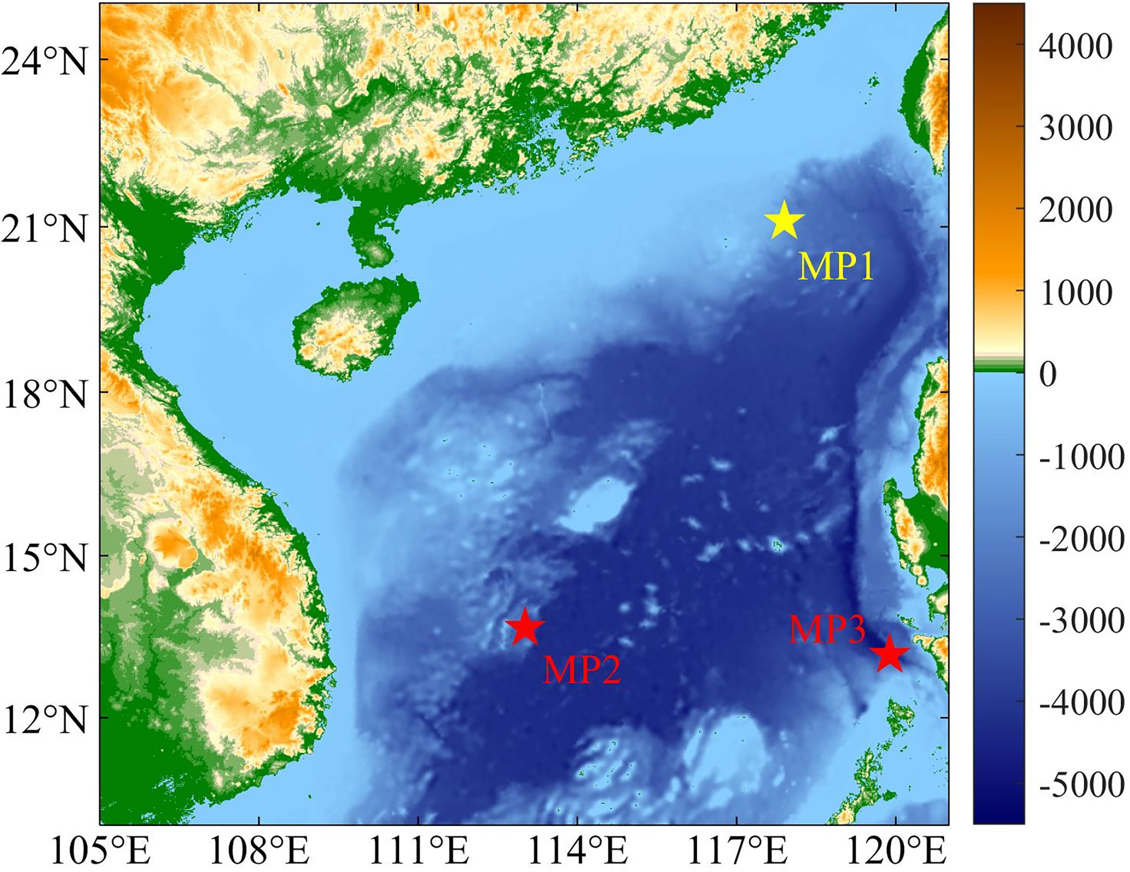
Figure 1 Topography and bathymetry of the SCS. The yellow star denotes the position of the mooring MP1 and two red stars denote two prescribed moorings of two ideal experiments.

FIGURE 2

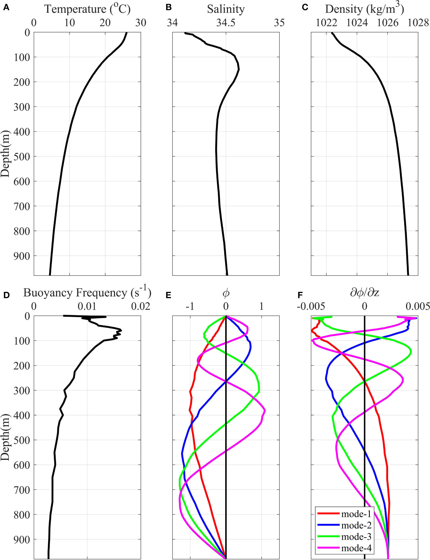
Figure 2 Spring (A) temperature, (B) salinity, and (C) density from WOA18 data at the mooring MP1. (D) Buoyancy frequency, and parts of (E) ϕ_m and (F) normal modes ∂ϕ_m/∂z at the mooring MP1.

2.2 Method to reconstruct full-depth tidal currents

In the ocean, ITs can be represented as a superposition of discrete baroclinic modes which depend on the buoyancy frequency. For horizontal tidal currents including barotropic tides and ITs, which is represented,

$\begin{array}{ll}\{\begin{array}{l}u(z,t)={\displaystyle \sum _{m=0}^{\infty }{u}_m}(z,t)={\displaystyle \sum _{m=0}^{\infty }\left[U_m(t)·\frac{\partial {\varphi }_m(z)}{\partial z}\right]}\hfill \\ v(z,t)={\displaystyle \sum _{m=0}^{\infty }{v}_m}(z,t)={\displaystyle \sum _{m=0}^{\infty }\left[V_m(t)·\frac{\partial {\varphi }_m(z)}{\partial z}\right]}\hfill \end{array},0<z<h& (1)\end{array}$

where u and v represent zonal and meridional current components of one tidal constituent (e.g. the M₂), z is depth, t is time, u_m and v_m are tidal current components of the m-th mode (m=0 represents the barotropic mode and m>0 represents the baroclinic mode), U_m and V_m are coefficients corresponding to u_m and v_m, respectively, and ϕ_m is eigenfunction of the eigenvalue problem. Refer to Appendix for the calculation of eigenfunctions.

Figures 2D–F displays the stratification and corresponding normal modes (∂ϕ_m/∂z) at the mooring MP1. Using the normal modes and the limited tidal current observations, U_m and V_m can be calculated with the least square method according to Equation 1. Then tidal currents of each mode can be calculated. By adding the barotropic tidal currents to all the baroclinic ones, the full-depth tidal currents are reconstructed.

3 Result

3.1 Reconstruction results with different observations at the mooring MP1

Cao et al. (2015) demonstrated that the observations from two ADCPs at the mooring MP1 can effectively reconstruct the full-depth M₂ tidal currents (through harmonic analysis) based on one barotropic mode and three baroclinic modes. Figure 3 shows the observed and reconstructed full-depth M₂ tidal currents as well as the barotropic and baroclinic tidal currents of each mode at the mooring MP1. Calculation of the horizontal kinetic energy density (HKE) of each mode shows that the M₂ tidal currents here are dominated by mode-1 (1830 J/m²) which accounts for 65.9% of the total HKE, followed by the barotropic mode (776 J/m²) explaining 27.9% of the total HKE. Higher modes account for smaller proportions with the mode-2 (150 J/m²) and mode-3 (23 J/m²) explaining 5.4% and 0.8% of the total HKE, respectively.

FIGURE 3

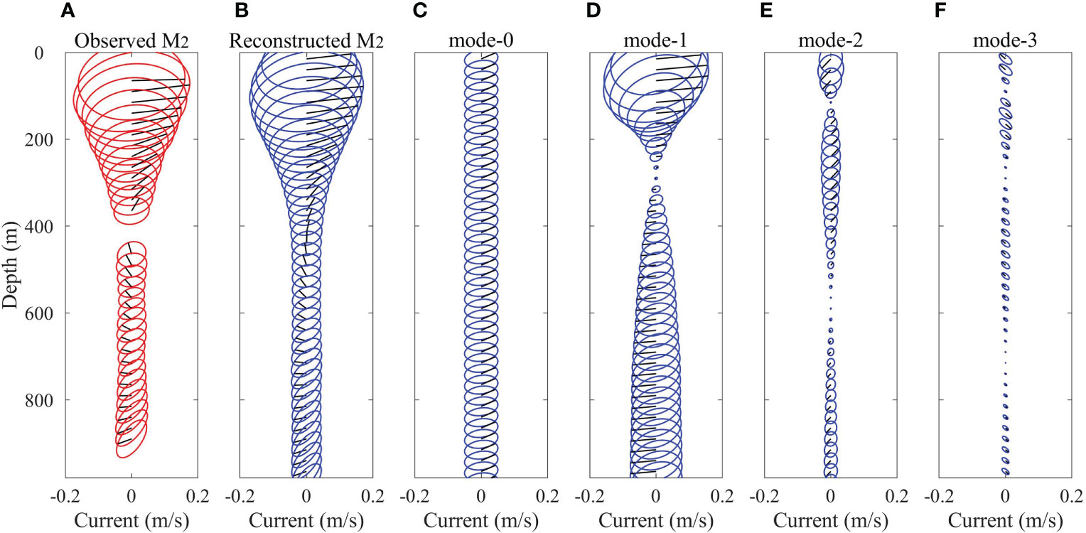
Figure 3 (A) Observed and (B) reconstructed M₂ tidal currents as well as (C-F) corresponding modes at the mooring MP1. Black lines in each subfigure represents the instantaneous currents at 01:00 local time (UTC+8) 1 Mar 2014.

In this paper, the less or simpler observations are used to try to effectively reconstruct full-depth M₂ tidal currents. 18 real experiments (REs) using different layers of ADCP data are carried out at the mooring MP1, of which details are displayed in Figure 4. It should be noted that one ADCP is replaced by several virtual CMs in all the REs except RE-1 and RE-2. Observations of virtual CMs are the real currents measured by ADCPs at the corresponding depth. Based on the modal analysis conducted in Cao et al (2015), one barotropic mode and three baroclinic modes are adopted in RE-1 to RE-18.

FIGURE 4

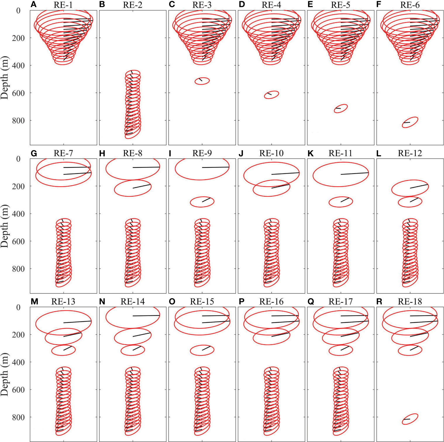
Figure 4 (A–R) Observed M₂ tidal currents in RE-1 to RE-18. The abscissa range is -0.2 m/s to 0.2 m/s. The depth layers of the virtual CMs measured by up-looking ADCP are 50, 100, 200 and 300 m, respectively. The depth layers of the virtual CMs measured by down-looking ADCP are 500, 600, 700 and 800 m, respectively.

Figure 5 illustrates reconstruction results of all REs. As can be seen from Figures 5A, B, when only observations from one ADCP are used, reconstructed tidal currents show obvious difference from the observed results (Figure 3B), especially at the depths outside the measuring range (e.g. 500-980 m in RE-1 and 0-500 m in RE-2). That indicates that it is nearly impossible to reproduce full-depth real tidal currents using only observations from one ADCP at the mooring MP1. Reconstructed tidal currents in RE-1 differ dramatically from those in RE-2. In RE-1, the error in reconstruction is mainly concentrated on the magnitude of currents below 500 m with reconstructed tidal currents being about triple larger than the real ones. While in RE-2, both amplitudes and phases show great differences between reconstructed tidal currents and the real ones outside the ADCP measuring range. In the upper 500 m, the amplitudes of reconstruction results are much larger than the real ones. Given that the least squares method is used in the reconstruction, it can be deduced that lack of essential observations results in the unreasonable reconstruction in RE-1 and RE-2. To evaluate the reconstructed results, mean absolute errors (MAEs) between amplitudes (phases) reconstructed with part of the observations and the observed results in each RE are shown in Table 1. As can be seen, the MAEs of amplitudes of u and v in RE-1 are much smaller than those in RE-2, while the MAEs of phases are larger than those in RE1-2. From the above statistics and Figures 5A, B, it can be concluded that the observations from the up-looking ADCP are more important than those from the down-looking one. The main reason is that tidal currents vary remarkably near the thermocline, which is within the measuring range of the up-looking ADCP.

FIGURE 5

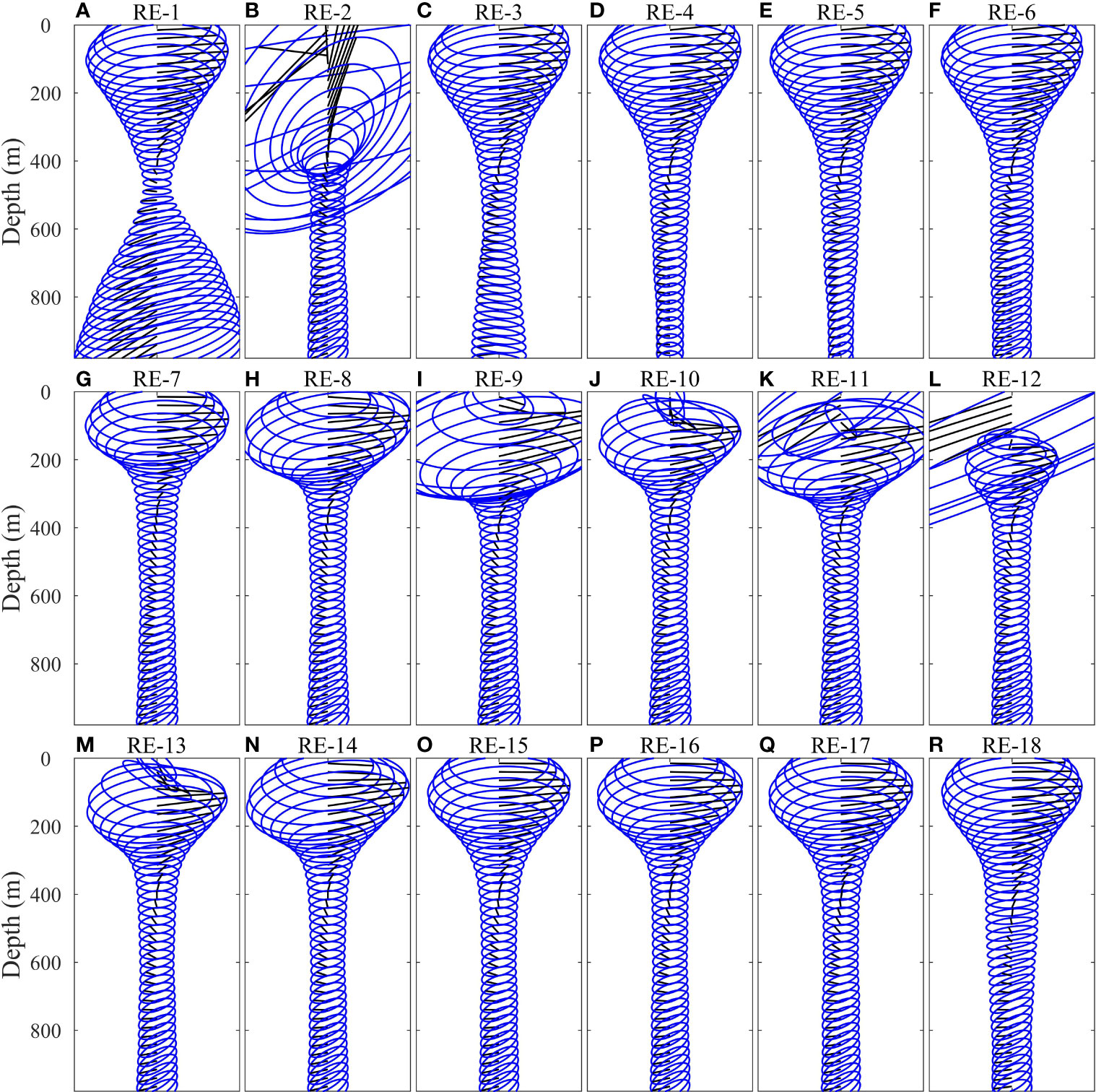
Figure 5 (A–R) Reconstructed M₂ tidal currents corresponding to RE-1 to RE-18 of Figure 4.

TABLE 1

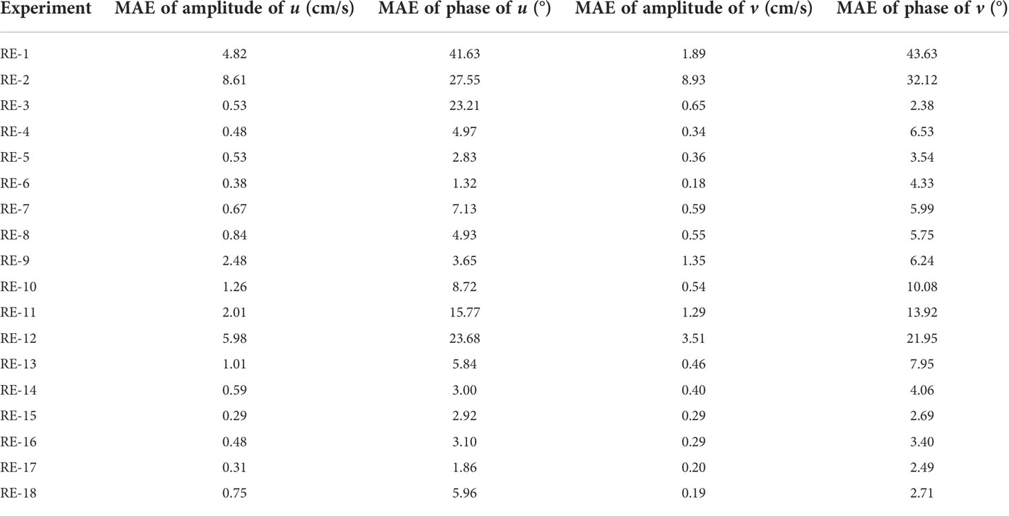
Table 1 MAEs of reconstructed tidal currents using part of the observations and the observed results in each experiment at the mooring MP1.

As discussed above, it is difficult to accurately reproduce the full-depth tidal currents at the mooring MP1 using only observations from one ADCP. Because the least square method is used in the reconstruction, adding observations may increase the accuracy of reconstruction results. Obviously, observations from two ADCPs are sufficient for perfect reconstruction. However, are all the observations from two ADCP essential? Would additional observations from several CMs besides those from one ADCP make reconstructed tidal currents more accurate? In order to investigate these problems, RE-3 to RE-18 are carried out. As can be seen from Figures 5C–F, when observations from both the up-looking ADCP and one virtual CM at 500 (600, 700, 800) m are used (from RE-3 to RE-6), the reconstructed tidal currents are close to the real ones. The result with one virtual CM at 800 m is closest to the real one (RE-6). The MAEs of amplitudes of u and v are 0.38 cm/s and 0.18 cm/s, which are much smaller than the precision of the 75kHz ADCP (0.50cm/s), and the MAEs of phases of u and v are 1.32° and 4.33°. Comparing the results from RE-3 to RE-6 (Table 1), with the increase of depth of the virtual CM, the reconstructed tidal currents are gradually approaching to the real ones. The result that the virtual CM is 400-500 m away from the up-looking ADCP (RE-6) is better than those of the other three schemes (from RE-3 to RE-5), suggesting that the observations of RE-6 are sufficient to obtain the real full-depth tidal currents at the mooring MP1. Results from RE-1 and RE-6 indicate the importance of observations in deep layer in the reconstruction of full-depth tidal currents.

However, tidal currents cannot be accurately reconstructed from the observations of the down-looking ADCP and two virtual CMs in the upper ocean (from RE-7 to RE-12), although their MAEs decrease compared with RE-2 (Table 1). Interestingly, changes of the depth of the two virtual CMs within the upper water column significantly influence the accuracy of reconstruction results. In RE-7 (RE-8) where the two virtual CMs are placed at 50 m and 100 m (200 m), compared with other schemes, the reconstruction results are closer to the real ones (Figures 5G, H). However, the MAEs of amplitude and phase are still large (Table 1, RE-7 and RE-8), the schemes are not sufficient to reconstruct the full-depth tidal currents effectively. In addition, in RE-9 to RE-12 where the two virtual CMs are placed at other depth, the real tidal currents cannot be reconstructed at all (Figures 5I–L). Even if tidal currents cannot be effectively reconstructed from observations of the down-looking ADCP and two virtual CMs, their results show that the CMs near the thermocline (50-200 m) play an important role in the reconstruction of full-depth tidal currents.

When three virtual CMs are used to replace the up-looking ADCP (Figures 4M–P), the results of RE-13 to RE-16 are shown in Figures 5M–P. In RE-15 (RE-16) where the three virtual CMs are placed at 50 m, 100 m and 300 m (200 m), the tidal currents can be reconstructed. The MAEs of amplitudes of u and v are smaller than 0.5 cm/s and the MAEs of phases of u and v are smaller than 4°. Compared with RE-7, adding only one more CM at 200 m or 300 m can make the results more accurate. Without CM at 50 m in RE-13 and without CM at 100 m in RE-14, although there are three CMs in these schemes, the results are still inaccurate, which indicates the importance of observation at depth near 50-100 m. When four virtual CMs replace the up-looking ADCP, the result in RE-17 is closest to real one (Figure 5Q). The MAEs of amplitudes of u and v in RE-17 are 0.31 cm/s and 0.20 cm/s and MAEs of phases of u and v are 1.86° and 2.49°.

Combining the results in RE-6 and RE-17, the real tidal currents can be reconstructed from the observations of the up-looking ADCP and one virtual CM at the depth layer of 800 m or from the observations of the down-looking ADCP and four virtual CMs at the depth layers of 50, 100, 200 and 300 m. The result with only five virtual CMs at 50, 100, 200, 300 and 800 m (RE-18) is shown in Figure 5R and the reconstructed tidal current is basically close to the real one in structure. The MAEs of amplitudes of u and v are 0.75 cm/s and 0.19 cm/s and the MAEs of phases of u and v are 5.96° and 2.71°. In addition to a high MAE of amplitude of u, other evaluations are within a reasonable range. This scheme is still feasible on purpose of saving costs.

As can be seen from Figure 2D, the buoyancy frequency has complex changes above 100 m, but it becomes regular to some extent below 100 m. Therefore, the CMs at 50-100 m are essential. The four virtual CMs at 50, 100, 200 and 300 m basically cover the most complex variation of the buoyancy frequency, which can replace an up-looking ADCP and can effectively reconstruct tidal currents. If the change of buoyancy frequency is not complex, fewer CMs can also reconstruct tidal current. The buoyancy frequency calculated by WOA05 is simpler than that calculated by WOA18 due to its low resolution. 2-3 virtual CMs can replace the up-looking ADCP and can effectively reconstruct tidal current with the buoyancy frequency calculated by WOA05 at the mooring MP1 (not shown). The real buoyancy frequency is more complex, and the thermocline coverage may be wider in other areas, so more CMs or an up-looking ADCP is inevitable. The number of CM depends on the complexity and range of buoyancy frequency variation.

Combing the results of the 18 experiments, it can be concluded that a) one ADCP measuring currents near the thermocline and one CM below 600 m are essential and sufficient to accurately reconstruct the full-depth tidal currents at the mooring MP1; b) four CMs (50, 100, 200 and 300 m) near the thermocline can basically replace an up-looking ADCP and more CMs are required in case of more complex variation of buoyancy frequency; c) four CMs near the thermocline and one CM below 600 m can basically reconstruct the full-depth tidal currents at the mooring MP1 in purpose of saving costs.

3.2 Reconstruction results with different observations at the moorings MP2 and MP3

In the deeper waters in the SCS, the structures of temperature, salinity and the buoyancy frequency will change, and the vertical structures of baroclinic modes are different from those at the mooring MP1. In order to explore the smallest number of necessary observations to reconstruct full-depth tidal currents accurately in deeper waters, two assumed moorings MP2 and MP3, where the water depths are 2500 m and 4300 m, are chosen for ideal experiments (IEs). For the universality of the experimental results, the moorings MP1, MP2 and MP3 are selected to be far apart (Figure 1) to obtain the structures of the temperature, salinity and the normal modes with great difference (Figure 6). The ideal data at the moorings MP2 and MP3 are prescribed as follows. 1) The coefficients U_m(t) and V_m(t) of one barotropic mode and ten baroclinic modes are obtained by modal decomposition and least square method at the mooring MP1. 2) One barotropic mode and ten baroclinic modes ∂ϕ_m/∂z are calculated at the moorings MP2 and MP3 using the temperatures and salinities from WOA18. 3) According to equation (1), the ideal M₂ tidal currents u(z,t) and v(z,t) are synthesized based on the 11 normal modes at the moorings MP2 and MP3 and the coefficients at the mooring MP1. 4) Adding the Gaussian white noise signals (regarded as measuring errors) to the ideal tidal currents, the prescribed full-depth M₂ tidal currents are obtained, which are regarded as “observations” in the IEs.

FIGURE 6

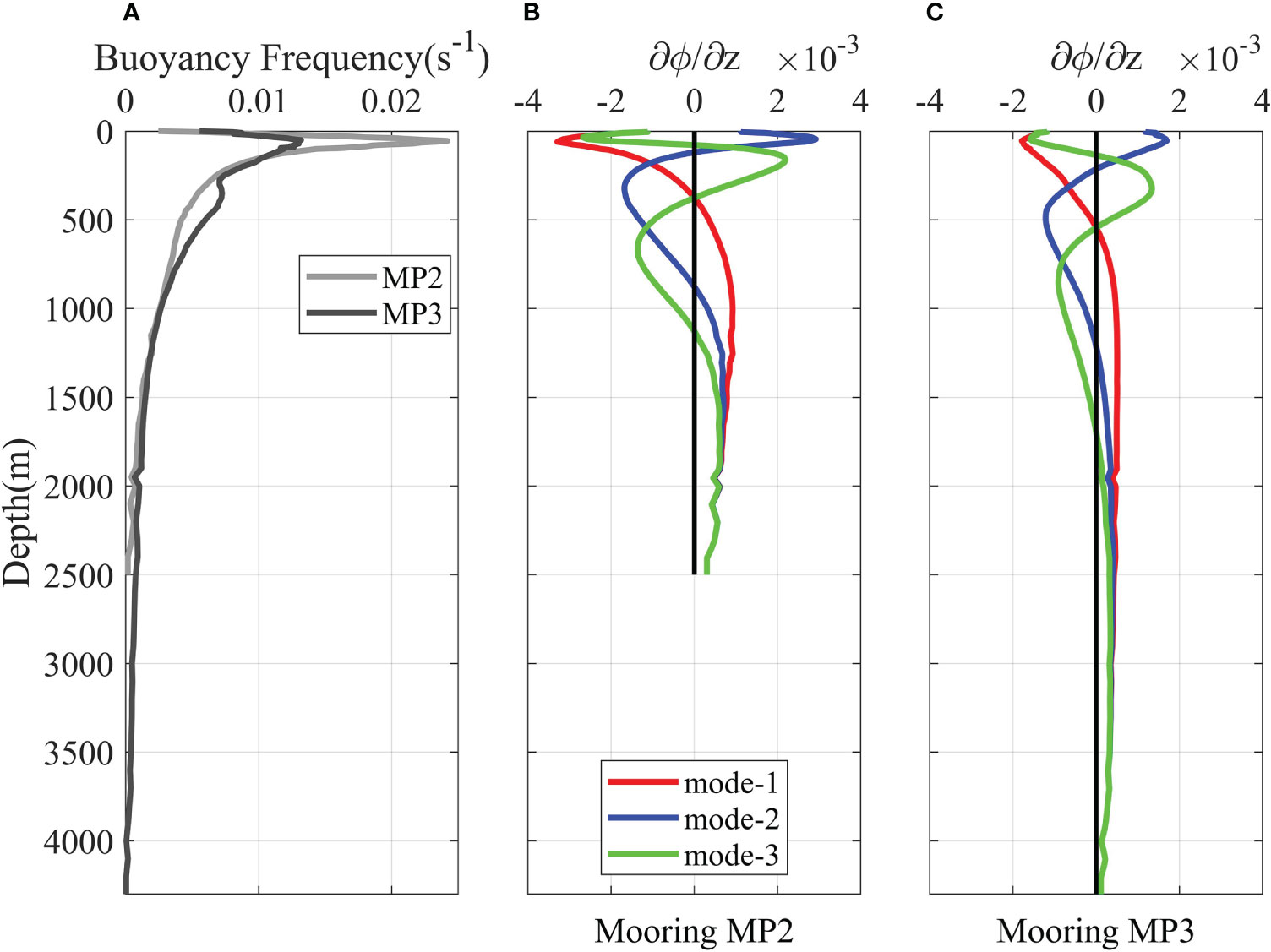
Figure 6 (A) Buoyancy frequency, and parts of (B, C) normal modes ∂ϕ_m/∂z at the moorings MP2 and MP3.

In equation (1), the coefficients U_m(t) and V_m(t) dominate the energy proportion of different normal modes and different tidal constituents. In the SCS, low modes account for larger proportions of HKE, and this paper focuses on the M₂ tidal constituents. Furthermore, the importance of the observation at different depth layers lies in the tidal current structure, that is, the modes calculated from the temperatures and salinities. Therefore, the coefficients at the mooring MP1 can be applied to the modes at the moorings MP2 and MP3.

3.2.1 Mooring MP2

The prescribed full-depth M₂ tidal currents, one barotropic tidal currents and three baroclinic mode currents at the mooring MP2 are shown in Figure 7. The vertical structure of tidal current at the mooring MP2 with 2500 m water depth is different from that at the mooring MP1 with 980 m water depth. The complex variation of amplitudes reaches around 200 m at the mooring MP2, while it reaches around 150 m at the mooring MP1. Below 2000 m at the mooring MP2, the M₂ has very small amplitudes and becomes rectilinear currents.

FIGURE 7

Figure 7 (A) Prescribed M₂ tidal currents in IEs at the mooring MP2, which are synthesized by (B) one prescribed barotropic modes and ten prescribed baroclinic modes. (C–E) Only the first three baroclinic modes are shown.

The smallest number of necessary observations to reconstruct full-depth tidal currents accurately is explored under this tidal current structure at the mooring MP2. In this experiment, we still use three baroclinic modes to reconstruct tidal observations (Cao et al., 2015), although they are synthesized by ten baroclinic modes. Through Section 3.1, we have realized the importance of up-looking ADCP for reconstructing full-depth tidal currents accurately. Based on this idea, ten IEs (Table 2) are designed, of which the up-looking ADCP is necessary.

TABLE 2

Table 2 Details of the IEs at the mooring MP2.

Table 3 lists the MAEs between the amplitudes (phases) reconstructed with part of the observations and those with all the observations in the ten IEs. In IE1-1, two ADCPs and four CMs with an interval of 500 m can effectively reconstruct the full-depth tidal current. The MAEs of amplitudes of u and v are both 0.16 cm/s, and the MAEs of phases of u and v are 5.86° and 9.38°. IE1-3 uses only the up-looking ADCP, resulting in a large MAE, which cannot reconstruct the tidal current at all. After adding a down-looking ADCP (IE1-2), the MAEs of phase of u and v are still large, and the MAE of phase of v reaches 31.25°. As can be seen from Figures 8A, B, the amplitudes of reconstructed tidal currents in IE1-2 are apparently smaller than the prescribed amplitudes (Figure 7A) below 1000 m due to lack of observations in the deep layer, suggesting that observations in the deep layer play an important role in the reconstruction. Then, on the basis of an up-looking ADCP, we explore the impact of adding different numbers of CMs on the reconstruction of full-depth tidal current. In IE1-4 to IE1-7 where one CM are placed at 1000 m, 1500 m, 2000 m and 2495 m respectively, the MAEs of IE1-5 and IE1-6 are much smaller than those of IE1-4 and IE1-7 (Table 3), and the observations of IE1-5 and IE1-6 have the ability to effectively reconstruct full-depth tidal current. It can be seen from Figures 8C, D that the reconstructed tidal current (IE1-5) is consistent with the prescribed M₂ tidal current (Figure 7A), which shows that the CMs in the middle of the deep layer (1500 m and 2000 m) are more important than that at the ends of the deep layer (1000 m and 2495 m).

TABLE 3

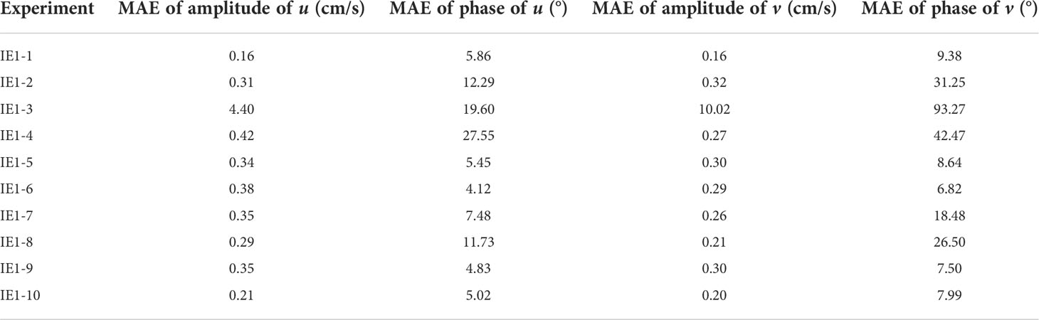
Table 3 MAEs of reconstructed tidal currents using part of the observations and prescribed tidal currents in each IE at the mooring MP2.

FIGURE 8

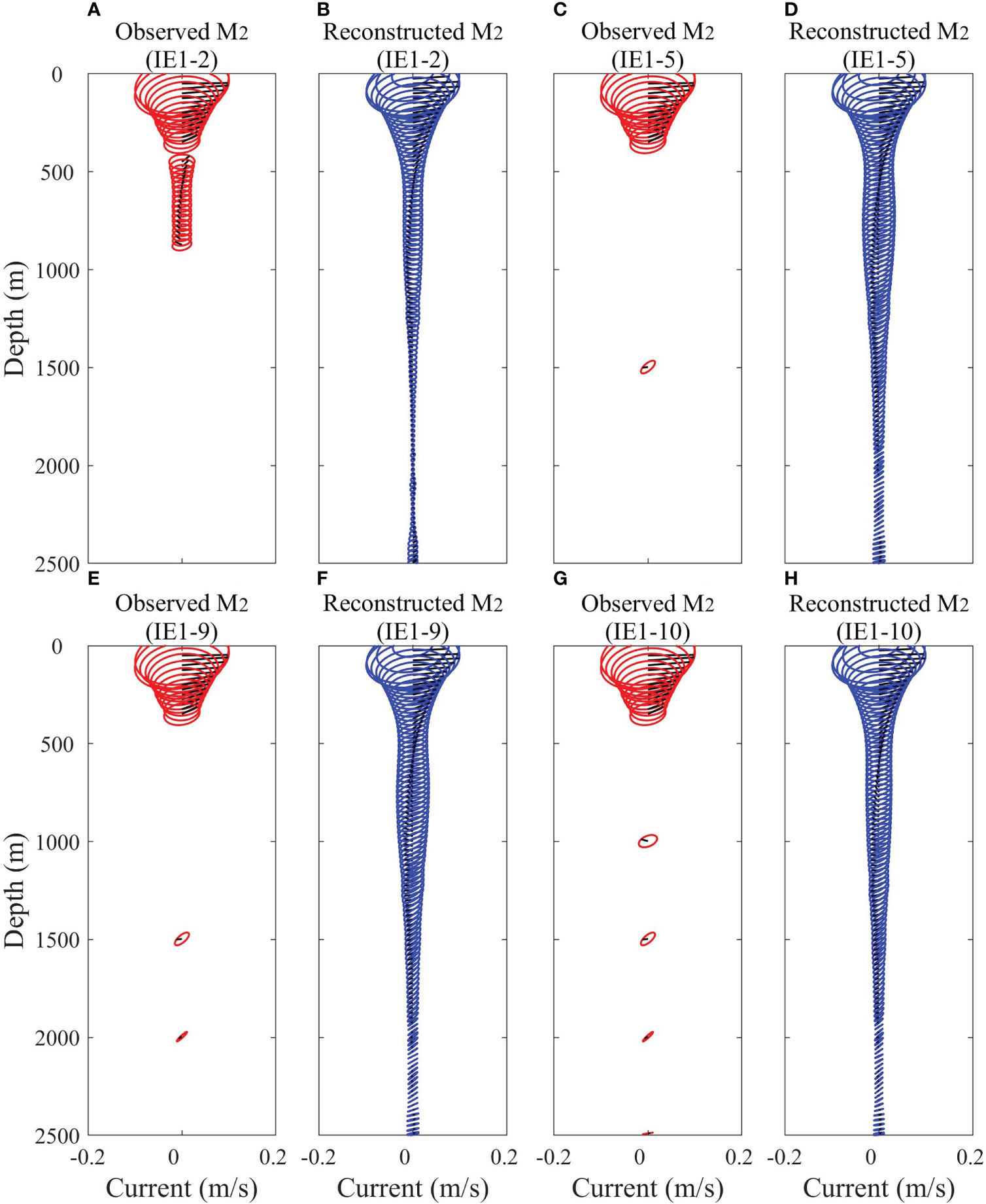
Figure 8 (A, C, E, G) Observed and (B, D, F, H) reconstructed M₂ tidal currents in (A, B) IE1-2, (C, D) IE1-5, (E, F) IE1-9 and (G, H) IE1-10.

Comparing the result of IE1-8 where two virtual CMs are placed at 1000 m and 2495 m and the result of IE1-9 where two virtual CMs are placed at 1500 m and 2000 m, it can be seen that even if two virtual CMs are used, the scheme of placing the CMs at two ends of the deep layer (IE1-8) cannot effectively reconstruct the tidal current. Due to the two CMs in the middle of the deep layer in IE1-9, the MAE is close to that in IE1-1 and is equivalent to those in IE1-5 and IE1-6. Figures 8E, F shows the observed and reconstructed M₂ tidal current in IE1-9. Once the observations from both the up-looking ADCP and four CMs with an interval of 500 m are used (IE1-10), the reconstructed tidal currents are the closest to those in IE1-1. Figures 8G, H shows the observed and reconstructed M₂ tidal current in IE1-10, indicating that the combination of observations from up-looking ADCP in the upper 500 m and four CMs at 1000-2500 m can well reconstruct the full-depth tidal current. In all IEs, the MAE of amplitude in IE1-1 has the smallest value, but the MAEs of phase of u and v in IE1-1 reach 5.86° and 9.38°, which are higher than those in some schemes without down-looking ADCP (IE1-5, IE1-6, IE1-9 and IE1-10). We speculate that although the amplitude varies remarkably in the upper 500 m, the variation of phase is not concentrated in some depths. Due to two ADCPs are added in the upper ocean, the fitting weights of least square method at 50-1000 m are much greater than those at 1000-2500 m, resulting in that the reconstruction of phase in IE1-1 is not as good as that in some schemes with relatively uniform observations.

3.2.2 Mooring MP3

Through the conclusions of Section 3.1 and Section 3.2.1, the importance of up-looking ADCP in the upper ocean and CMs in the deep layer cannot be ignored for reconstructing full-depth tidal currents accurately. At the mooring MP3 where the water depth is 4300 m, five IEs are carried out (Table 4). In IE2-1, two ADCPs cover 50-1000 m and seven CMs with an interval of 500 m cover 1000-4000 m. The MAEs of amplitudes of u and v are only 0.07 cm/s, and the MAEs of phases of u and v are 3.46° and 9.41° (Table 5), which can reconstruct the full-depth tidal currents accurately. Regarding the MAEs in IE2-1 as a relative standard, the reconstructed tidal currents with fewer CMs are explored. In IE2-2, the down-looking ADCP is replaced by one CM at 500 m on the basis of IE2-1 (Figures 9A, B). Its MAEs are very close to those in IE1-1. The MAEs of amplitudes of u and v increase only 0.01 cm/s, and the MAEs of phases of u and v increases less than 2°. When half of the CMs are removed on the basis of IE2-2 (i.e., four CMs with an interval of 1000 m are placed at 1000 m, 2000 m, 3000 m and 4000 m in IE2-3, Figures 9D, E), the result is still acceptable. The MAEs of amplitudes of u and v are 0.11 cm/s and 0.09 cm/s, and MAEs of phases of u and v are 5.18° and 13.90°. When only two CMs are used (IE2-4 and IE2-5), the results are worse than other experiments, and their MAEs of phases of v reach 23.11° and 19.50°, respectively. Similarly, the result of IE2-4 is better than that of IE2-5, which also confirms the conclusion of the previous chapter that the CMs in the middle of the deep layer are more important than that at the ends of the deep layer.

TABLE 4

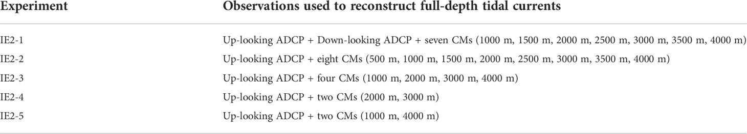
Table 4 Details of IEs at the mooring MP3.

TABLE 5

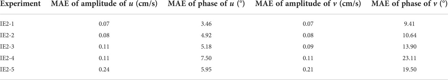
Table 5 MAEs of reconstructed tidal currents using part of the observations and prescribed tidal currents in each IE at the mooring MP3.

FIGURE 9

Figure 9 (A, D) Observed and (B, C, E, F) reconstructed M₂ tidal currents with (B, E) four normal modes and (C, F) ten normal modes in (A–C) IE2-2 and (D–F) IE2-3.

From the above results, it indicates that the full-depth tidal current can be accurately reconstructed by using an up-looking ADCP and four CMs with an interval of 1000 m (IE2-3). Even if only two CMs at 2000 m and 3000 m are used (IE2-4), the MAEs of amplitudes of u and v are still very small (0.11 cm/s). This is because the tidal ellipse does not change remarkably below 1000 m (Figures 8H; 9B), no matter at the mooring MP2 with 2500 m water depth or MP3 with 4300 m water depth. In addition, only one barotropic mode and first three baroclinic modes are used in the fitting process, and the low-mode baroclinic motions changes slowly, resulting in low degrees of freedom. As long as there are a few observations below 1000 m, the result will be close to real tidal currents. Generally speaking, the tidal current is dominated by barotropic modes and the first two baroclinic modes. Higher modes account for smaller proportions of the total HKE, because the high-mode baroclinic motions are easy to dissipate (Nikurashin and Legg, 2011). However, the energy of high-mode may not be ignored in some sea area. Considering more modes will increase the universality of this study and make the results more accurate.

We performed a sensitivity experiment for the five IEs listed in Table 4, where the mode number increases gradually from 2 (one barotropic mode and one baroclinic mode) to 11 (one barotropic mode and ten baroclinic modes). The MAEs of amplitudes and phases of u and v for the five IEs are shown in Figure 10. The MAEs are quite similar in the five IEs with 4 modes, except for phase of v. However, with the increase of mode number, there are large MAEs between the results of IE2-4 and IE2-5 with two CMs and the real tidal currents with 5 or 6 modes, and there are large MAEs between the result of IE2-3 with four CMs and the real tidal currents with 10 modes. Figure 9F shows the reconstructed tidal current in IE2-3 when the mode number is 10. With ten normal modes, the scheme of the four CMs with an interval of 1000 m cannot reconstruct the tidal current accurately, which has considerable MAEs of amplitude and phase. Only IE2-1 and IE2-2 are insensitive to the increase of mode number, and the results show a convergence trend. With ten normal modes in IE2-2 (Figure 9C), the MAEs of amplitudes of u and v are 0.04 cm/s and 0.07 cm/s, and the MAEs of phases of u and v are 1.7° and 3.6°, which have smaller MAEs than that in Table 5 using four normal modes. As discussed above, we conclude that if four normal modes are considered, an up-looking ADCP and several CMs with an interval of 1000 m can reconstruct full-depth tidal current accurately. If more modes need to be considered to deal with high-mode baroclinic motions, it is better to use an up-looking ADCP and several CMs with an interval of 500 m.

FIGURE 10

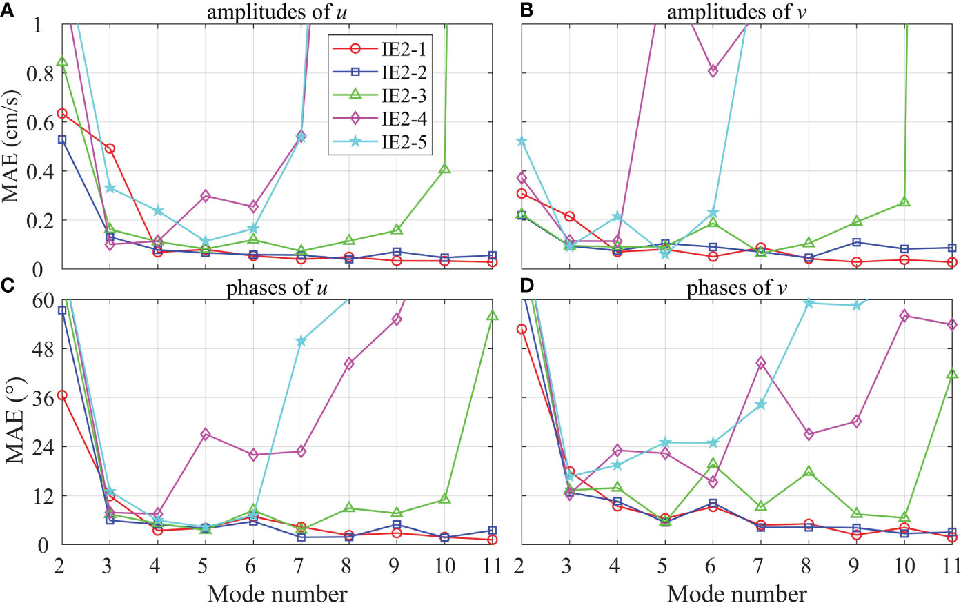
Figure 10 The MAEs of amplitudes of (A) u and (B) v from IE2-1 to IE2-5 at the mooring MP3 with different mode number, and the MAEs of phases of (C) u and (D) v from IE2-1 to IE2-5 at the mooring MP3 with different mode number.

4 Discussion and conclusions

In this study, we explore how many observations are sufficient and essential to reconstruct full-depth tidal currents based on the modal decomposition and least square method. A series of experiments are carried out based on direct observations at the mooring MP1 and synthetic observations at moorings MP2 and MP3 in the SCS. Combing the results at the three moorings, we can make some generalized conclusions.

Fundamentally, both observations in the upper ocean (especially near the thermocline) and deep layer are essential for the reconstruction of full-depth tidal currents. The observations from the up-looking ADCP are more important than those from the down-looking one. The main reason is that tidal currents vary remarkably near the thermocline, which is within the measuring range of the up-looking ADCP

For the upper ocean, at least 2-4 CMs are required to replace an up-looking ADCP near the thermocline, and it is important to place those CMs at the depth where the buoyancy frequency have complex variation. In different areas, the depth of thermocline may change, so more CMs are needed to replace an up-looking ADCP with deeper thermocline. The number of CM in the upper ocean depends on the complexity and range of buoyancy frequency variation. Therefore, an up-looking ADCP is generally necessary.

For the deep layer, more observations are needed as water depth increases. Based on the observations from an up-looking ADCP for the stations with water depths less than 1000 m, increasing one CM at in the middle of the deep layer can effectively reconstruct full-depth tidal currents based on one barotropic mode and three baroclinic modes. Due to the small changes of tidal ellipses and buoyancy frequencies in the deep layer, the increase of water depth does not have a linear relationship with the increase of the smallest number of CMs. At the mooing MP2 with depth of 2500 m, increasing four CMs with an interval of 500 m (IE1-10) in the deep layer can make the reconstruction result accurate enough. At the mooing MP3 with depth of 4300 m, increasing four CMs with an interval of 1000 m (IE2-3) in the deep layer can make the reconstruction result accurate enough. They have a similar characteristic, that is, their CM interval/water depth ratios are approximately equal to 0.2. The parameter may be useful for the design of moorings with different water depths to obtain full-depth tidal currents. Significantly, the CMs in the middle of the deep layer are more important than that at two ends of the deep layer, such as RE-6 (800 m) at the mooring MP1, IE1-5 (1500 m), IE1-6 (2000 m), and IE1-9 (1500 and 2000 m) at the mooring MP2, and IE2-4 (2000 and 3000 m) at the mooring MP3. This design may be more cost-effective at a small loss of accuracy. Considering the generality, if there was high-mode energy of tidal currents at the mooring MP3, an up-looking ADCP in the upper ocean (especially near the thermocline) and seven CMs with an interval of 500 m in the deep layer can accurately reconstruct the full-depth tidal currents, i.e., the CM interval/water depth ratios should be at least less than 1/8 to avoid higher-mode fits unstable in the modal decomposition.

Data availability statement

This dataset will not be authorized. Requests to access the datasets should be directed to YW, wangyuzhe@stu.ouc.edu.cn.

Author contributions

YW, JW, and XL contributed to conception and design of the study. YW wrote the first draft of the manuscript. YZ wrote sections of the manuscript. All authors contributed to manuscript revision, read, and approved the submitted version.

Funding

This work is supported by the National Natural Science Foundation of China (Grant Nos. 42076011, U1806214 and 41706012), the Natural Science Foundation of Shandong Province of China (Grant No. ZR2020mD056), the National Key Research and Development Project of China (Grant No. 2019YFC1408405), the Open Fund Project of Key Laboratory of Marine Environmental Information Technology, Ministry of Natural Resources of the People’s Republic of China.

Conflict of interest

The authors declare that the research was conducted in the absence of any commercial or financial relationships that could be construed as a potential conflict of interest.

Publisher’s note

All claims expressed in this article are solely those of the authors and do not necessarily represent those of their affiliated organizations, or those of the publisher, the editors and the reviewers. Any product that may be evaluated in this article, or claim that may be made by its manufacturer, is not guaranteed or endorsed by the publisher.

References

Alford M. H., Mackinnon J. A., Nash J. D., Simmons H., Pickering A., Klymak J. M., et al. (2011). Energy flux and dissipation in luzon strait: Two tales of two ridges. J. Phys. Oceanogr. 41, 2211–2222. doi: 10.1175/JPO-D-11-073.1

CrossRef Full Text | Google Scholar

Alford M. H., Peacock T., Mackinnon J. A., Nash J. D., Buijsman M. C., Centuroni L. R., et al. (2015). The formation and fate of internal waves in the south China Sea. Nature 521, 65–69. doi: 10.1038/nature14399

PubMed Abstract | CrossRef Full Text | Google Scholar

Boyer T. P., Garcia H. E., Locarnini R. A., Zweng M. M., Mishonov A. V., Reagan J. R., et al. (2018) World Ocean Atlas 2018. [Temperature and Salinity]. NOAA National Centers for Environmental Information. Dataset. Available at: https://www.ncei.noaa.gov/archive/accession/NCEI-WOA18. Accessed [15/5/2022].

Google Scholar

Buijsman M. C., Klymak J. M., Legg S., Alford M. H., Farmer D., Mackinnon J. A., et al. (2014). Three-dimensional double-ridge internal tide resonance in luzon strait. J. Phys. Oceanogr. 44, 850–869. doi: 10.1175/JPO-D-13-024.1

CrossRef Full Text | Google Scholar

Buijsman M. C., Legg S., Klymak J. (2012). Double-ridge internal tide interference and its effect on dissipation in Luzon strait. J. Phys. Oceanogr. 42, 1337–1356. doi: 10.1175/JPO-D-11-0210.1

CrossRef Full Text | Google Scholar

Cao A. Z., Li B. T., Lv X. Q. (2015). Extraction of internal tidal currents and reconstruction of full-depth tidal currents from mooring observations. J. Atmos. Ocean. Technol. 32, 1414–1424. doi: 10.1175/JTECH-D-14-00221.1

CrossRef Full Text | Google Scholar

Chao S. Y., Ko D. S., Lien R. C., Shaw P. T. (2007). Assessing the west ridge of Luzon strait as an internal wave mediator. J. Oceanogr. 63, 897–911. doi: 10.1007/s10872-007-0076-8

CrossRef Full Text | Google Scholar

Costa F. B., Tanajura C. A. S. (2022). On the impact of vertical coordinate choice for innovation when assimilating hydrographic profiles into isopycnal ocean models. Ocean Model. 169, 101917. doi: 10.1016/j.ocemod.2021.101917

CrossRef Full Text | Google Scholar

Dunphy M., Lamb K. G. (2014). Focusing and vertical mode scattering of the first mode internal tide by mesoscale eddy interaction. J. Geophys. Res. Ocean. 119, 523–536. doi: 10.1002/2013JC009293

CrossRef Full Text | Google Scholar

Egbert G. D., Ray R. D. (2000). Significant dissipation of tidal energy in the deep ocean inferred from satellite altimeter data. Nature 405, 775–778. doi: 10.1038/35015531

PubMed Abstract | CrossRef Full Text | Google Scholar

Gouretski V. (2018). World ocean circulation experiment-argo global hydrographic climatology. Ocean Sci. 14, 1127–1146. doi: 10.5194/os-14-1127-2018

CrossRef Full Text | Google Scholar

Guan S., Zhao W., Huthnance J., Tian J., Wang J. (2014). Observed upper ocean response to typhoon megi, (2010) in the northern south China Sea. J. Geophys. Res. Ocean 119, 3134–3157. doi: 10.1002/2013JC009661

CrossRef Full Text | Google Scholar

Guo P., Fang W., Liu C., Qiu F. (2012). Seasonal characteristics of internal tides on the continental shelf in the northern south China Sea. J. Geophys. Res. Ocean. 117, C04023. doi: 10.1029/2011JC007215

CrossRef Full Text | Google Scholar

Jan S., Chern C.-S., Wang J., and Chao S.-Y. (2007). Generation of diurnal K 1 internal tide in the Luzon Strait and its influence on surface tide in the South China Sea. J. Geophys. Res. 112, C06019. doi: 10.1029/2006JC004003

CrossRef Full Text | Google Scholar

Katsumata K., Wijffels S. E., Steinberg C. R., Brinkman R. (2010). Variability of the semidiurnal internal tides observed on the timor shelf. J. Geophys. Res. Ocean. 115, 2009JC006071. doi: 10.1029/2009JC006071

CrossRef Full Text | Google Scholar

Li B., Du L., Peng S., Yuan Y., Meng X., Lv X. (2021). Modulation of internal tides by turbulent mixing in the south China Sea. Front. Mar. Sci. 8. doi: 10.3389/fmars.2021.772979

PubMed Abstract | CrossRef Full Text | Google Scholar

Li H., Xu F., Zhou W., Wang D., Wright J. S., Liu Z., et al. (2017). Development of a global gridded argo data set with Barnes successive corrections. J. Geophys. Res. Ocean. 122, 866–889. doi: 10.1002/2016JC012285

CrossRef Full Text | Google Scholar

Munk W. (1997). Once again: once again–tidal friction. Prog. Oceanogr. 40, 7–35. doi: 10.1016/S0079-6611(97)00021-9

CrossRef Full Text | Google Scholar

Nash J. D., Alford M. H., Kunze E. (2005). Estimating internal wave energy fluxes in the ocean. J. Atmos. Ocean. Technol. 22, 1551–1570. doi: 10.1175/JTECH1784.1

CrossRef Full Text | Google Scholar

Nikurashin M., Legg S. (2011). A mechanism for local dissipation of internal tides generated at rough topography. J. Phys. Oceanogr. 41, 378–395. doi: 10.1175/2010JPO4522.1

CrossRef Full Text | Google Scholar

Niwa Y., Hibiya T. (2001). Numerical study of the spatial distribution of the M2 internal tide in the pacific ocean. J. Geophys. Res. Ocean. 106, 22441–22449. doi: 10.1029/2000jc000770

CrossRef Full Text | Google Scholar

Rudnick D. L., Boyd T. J., Brainard R. E., Carter G. S., Egbert G. D., Gregg M. C., et al. (2003). From tides to mixing along the Hawaiian ridge. Sci. (80-. ). 301, 355–357. doi: 10.1126/science.1085837

CrossRef Full Text | Google Scholar

Shang X., Liu Q., Xie X., Chen G., Chen R. (2015). Characteristics and seasonal variability of internal tides in the southern south China Sea. Deep. Res. Part I Oceanogr. Res. Pap. 98, 43–52. doi: 10.1016/j.dsr.2014.12.005

CrossRef Full Text | Google Scholar

Simmons H. L., Hallberg R. W., Arbic B. K. (2004). Internal wave generation in a global baroclinic tide model. Deep. Res. Part II Top. Stud. Oceanogr. 51, 3043–3068. doi: 10.1016/j.dsr2.2004.09.015

CrossRef Full Text | Google Scholar

Tian J., Yang Q., Zhsao W. (2009). Enhanced diapycnal mixing in the south China Sea. J. Phys. Oceanogr. 39, 3191–3203. doi: 10.1175/2009JPO3899.1

CrossRef Full Text | Google Scholar

Wang S., Chen X., Wang J., Li Q., Meng J., Xu Y. (2019). Scattering of low-mode internal tides at a continental shelf. J. Phys. Oceanogr. 49, 453–468. doi: 10.1175/JPO-D-18-0179.1

CrossRef Full Text | Google Scholar

Wang J., Yu F., Nan F., Ren Q., Chen Z., Zheng T. (2021). Observed three dimensional distributions of enhanced turbulence near the Luzon strait. Sci. Rep. 11, 14835. doi: 10.1038/s41598-021-94223-3

PubMed Abstract | CrossRef Full Text | Google Scholar

Xie X., Liu Q., Zhao Z., Shang X., Cai S., Wang D., et al. (2018). Deep Sea currents driven by breaking internal tides on the continental slope. Geophys. Res. Lett. 45, 6160–6166. doi: 10.1029/2018GL078372

CrossRef Full Text | Google Scholar

Xu Z., Yin B., Hou Y., Xu Y. (2013). Variability of internal tides and near-inertial waves on the continental slope of the Northwestern South China Sea. J. Geophys. Res. Ocean. 118, 197–211. doi: 10.1029/2012JC008212

CrossRef Full Text | Google Scholar

Zhang Z., Tian J., Qiu B., Zhao W., Chang P., Wu D., et al. (2016). Observed 3D structure, generation, and dissipation of oceanic mesoscale eddies in the south China Sea. Sci. Rep. 6, 24349. doi: 10.1038/srep24349

PubMed Abstract | CrossRef Full Text | Google Scholar

Zhao Z. (2014). Internal tide radiation from the Luzon strait. J. Geophys. Res. Ocean. 119, 5434–5448. doi: 10.1002/2014jc010014

CrossRef Full Text | Google Scholar

Zhao Z., Alford M. H., Mackinnon J. A., Pinkel R. (2010). Long-range propagation of the semidiurnal internal tide from the Hawaiian ridge. J. Phys. Oceanogr. 40, 713–736. doi: 10.1175/2009JPO4207.1

CrossRef Full Text | Google Scholar

Appendix: Calculation of eigenfunctions

ϕ_m are eigenfunctions of the eigenvalue problem for wave speed c:

$\begin{array}{ll}\begin{array}{l}\frac{{\partial }^2\varphi }{\partial z^2}+\frac{N^2}{c^2}\varphi =0\\ \varphi =0\text{\hspace{1em} at \hspace{1em}}z=0\\ \varphi =0\text{\hspace{1em} at \hspace{1em}}z=h\end{array}& \text{(A1)}\end{array}$

where N is buoyancy frequency and h is water depth. Refer to Zhao et al. (2010) and Cao et al. (2015), the eigenfunctions should satisfy an orthogonality condition:

$\begin{array}{ll}{\displaystyle {\int }_0^h\frac{\partial {\varphi }_m}{\partial z}}\frac{\partial {\varphi }_n}{\partial z}dz=\{\begin{array}{ll}0\hfill & n\ne m\hfill \\ I\hfill & n=m\hfill \end{array}& \text{(A2)}\end{array}$

According to Griffiths and Grimshaw (2007), for the barotropic mode,

$\begin{array}{ll}\begin{array}{l}{c}_0=\sqrt{gh}\\ {\varphi }_0=1+z/h\end{array}& \text{(A3)}\end{array}$

where g is the gravitational acceleration. Basing on the Wentzel–Kramers–Brillouin (WKB) approximation, the baroclinic modes can be calculated by taking

$\begin{array}{ll}I={\pi }^2/2h& \text{(A4)}\end{array}$

and the corresponding eigenvalues and eigenfunctions are

$\begin{array}{ll}\begin{array}{l}{c}_m\approx c_m^{\text{WKB}}=\frac{\overline{N}h}{m\pi }\\ {\varphi }_m\approx {\varphi }_m^{\text{WKB}}=\frac{{(-1)}^m}{m}\sqrt{\frac{\overline{N}}{N}}\sin \left[\frac{m\pi }{\overline{N}h}{\displaystyle {\int }_0^{z}N}\left(z^{\prime }\right)d{z}^{\prime }\right]\end{array}& \text{(A5)}\end{array}$

Where

$\begin{array}{ll}\overline{N}\equiv \frac{1}{h}{\displaystyle {\int }_0^{h}N}(z)dz& \text{(A6)}\end{array}$

is the depth-averaged buoyancy frequency. Then, the normal modes in Equation (1) can be calculated as

$\begin{array}{ll}\begin{array}{l}\frac{\partial {\varphi }_0}{\partial z}=\frac{1}{h}\\ \frac{\partial {\varphi }_m}{\partial z}=\frac{{(-1)}^m\pi }{h}\sqrt{\frac{N}{\overline{N}}}\cos \left[\frac{m\pi }{\overline{N}h}{\displaystyle {\int }_0^{z}N}\left(z^{\prime }\right)d{z}^{\prime }\right]\end{array}& \text{(A7)}\end{array}$