 Luiz Alexandre A. Guerra
 Guilherme N. Mill
 Afonso M. Paiva
- 1PETROBRAS/CENPES, Cidade Universitária, Rio de Janeiro, Brazil
- 2Programa de Engenharia Oceânica – PEnO/COPPE, Universidade Federal do Rio de Janeiro (UFRJ), Centro de Tecnologia, Cidade Universitária, Rio de Janeiro, Brazil
- 3Centre of Excellence, Vale S.A. - Vitória, Espírito Santo, Brazil
The Agulhas rings transport warm and salty waters that feed the surface limb of the Atlantic Meridional Overturning Circulation. Some studies have focused on the conveying capacity of ocean eddies, and recently, the role of the Agulhas rings in advecting water masses and organisms has been explored. Here we show evidence that the Agulhas rings are responsible for the advection of mode waters from the Cape Basin to the western side of the Atlantic. We analyzed more than 3,200 temperature profiles and 2,400 salinity profiles from historical databases collocated with 52 long-lived Agulhas rings tracked from 1993 through 2016. An automated algorithm was used to identify thermostads in the profiles acquired within the rings. The data revealed mode water layers trapped inside 88% of the rings. The joint distribution of temperature and salinity indicated two types of mode waters in the range 16.2 ± 0.6°C, 35.6 ± 0.1 (Type I) and 12.9 ± 0.7°C, 35.2 ± 0.1 (Type II). The majority (67%) of the rings carrying mode waters had both types detected inside. Moreover, considering only those rings sampled west of the Mid-Atlantic Ridge, we found that 45% of them advected mode waters to the western basin. Therefore, our results demonstrate that, despite the long journey, interaction with the bottom topography and other vortices, ocean-atmosphere exchanges, and decay, the Agulhas rings are responsible for spreading mode waters initially available at the Cape Basin throughout the South Atlantic, contributing to a positive anomaly in temperature and salinity along the eddy corridor joining the Cape Basin to the Brazil Basin.
1. Introduction
The Agulhas Leakage refers to the transferring of warm and salty Indian Ocean waters into the Atlantic, whose main component is the spawning of anticyclonic rings from the retroflection of the Agulhas Current that takes place south of Africa (de Ruijter and Boudra, 1985; Gordon, 1985; Gordon, 1986; Lutjeharms and Gordon, 1987; Lutjeharms and van Ballegooyen, 1988; Lutjeharms, 1996; de Ruijter et al., 1999; Richardson, 2007).
Several studies have explored the role of the Great Agulhas System on the Earth's climate. The retroflection works like a gateway to the warm return flow of the Atlantic Meridional Overturning Circulation (AMOC) (de Ruijter et al., 1999; Beal et al., 2011). So as the retroflection behavior depends on its position, determined by the wind field, the leakage variability has been known to range from interannual to decadal periods (Witter and Gordon, 1999; Biastoch et al., 2009; van Sebille et al., 2009; Backeberg et al., 2012). As an example, Rouault et al. (2009) point out that since the 1980s, a temperature increase in the Agulhas system has been observed due to the wind’s intensification with maximum southward displacement. The increased leakage has implications for stabilizing the AMOC, which may counterpoint a trend toward weakening the thermohaline circulation in a scenario of glaciers melting in Greenland (Weijer et al., 2002; Beal et al., 2011).
Fossil records from the Cape Basin indicate that the exchanges between the Indian and Atlantic oceans have been highly variable, alternating water cooling during glacial periods and warming in interglacial intervals in the last 450,000 years (Rau et al., 2002). Some studies have suggested that the onset of an increased Agulhas Leakage is crucial in glacial terminations resulting in a resumption of the AMOC (Peeters et al., 2004). However, there was doubt due to a lack of evidence of leakage spread reaching the West and eventual deep-water convection in the North Atlantic. Recently, Ballalai et al. (2019) put forward the results of a comparative analysis of a new fossil record from the Brazilian coast and another from the Cape Basin, which suggest a common mechanism responsible for increasing the salinity on both sides of the Atlantic. The authors proposed that the observed salinity anomaly responded to an increased Agulhas Leakage through Agulhas rings’ progression connecting both sides of the Atlantic. The arrival of Agulhas rings to the western border, once hypothesized (Gordon and Haxby, 1990; Byrne et al., 1995; Nof, 1999; Azevedo et al., 2012), was recently confirmed with in situ evidence by Guerra et al. (2018). Subsequently, Laxenaire et al. (2018) conducted research on the role of Agulhas rings connecting the western boundaries of the Indian and Atlantic Oceans, using a new technique for eddy tracking that keeps records of merging and split-off events.
Vortices are well known for their capacity for transporting heat, mass, and other scalars trapped in the inner core, isolated from the external world (Danabasoglu et al., 1994; Volkov et al., 2008; Dong et al., 2014; Jayne and Marotzke, 2002; Souza et al., 2011; Zhang et al., 2014; Wang et al., 2015). Even though Agulhas rings experience an exponential decay, with a reduction of ~80% in amplitude within a year after shedding (Byrne et al., 1995; Schouten et al., 2000; van Sebille et al., 2010; Guerra et al., 2018), many studies have identified mode waters inside rings in the Cape Basin and beyond the Walvis Ridge at the Mid-Atlantic (McCartney and Woodgate-Jones, 1991; Olson et al., 1992; Toole and Warren, 1993; McDonagh et al., 2005; Guerra, 2011). New estimates of the transport of Agulhas rings heat content showed that most heat anomalies are associated with the mode water layers advected westward during the rings translation along the South Atlantic (Laxenaire et al., 2020).
Mode waters (MWs) are vertical homogeneous layers of the thermocline waters formed by subduction from the mixed layer during wintertime conditions (Hanawa and Talley, 2001). Different types of MW have been identified and described in the literature in the South Atlantic. The South Atlantic Central Water comprises three MWs with distinct ranges of properties (Provost et al., 1999; Sato and Polito, 2014). Each MW was observed in different regions of the subtropical gyre: the western side of the gyre near the Brazil Current recirculation, the southern edge of the gyre in the central and eastern South Atlantic, and on the east side of the basin, including the Cape Basin region (Sato and Polito, 2014; Bernardo and Sato, 2020).While it is generally agreed that there are three varieties of subtropical MW (STMW) in the South Atlantic, there is less consensus over whether or not they are influenced by remote central waters or locally formed. De Souza et al. (2018) revisited data from WOCE cruises and Argo floats and found an important contribution of the Subtropical Indian MW (SIMW) in the thermocline waters of the South Atlantic. Surprisingly, the presence of the SIMW increased westward, and the authors suggested that this tendency was related to the advection of Indian MW trapped inside Agulhas rings as they traveled westward. Using numerical modeling, Capuano et al. (2018) demonstrated the role of turbulence and instabilities in the Cape Basin on the transformation of water masses from the Indian Ocean and subduction of MW inside Agulhas rings. Using a new algorithm to detect MW in Argo profiles, including outcropping MW, Chen et al. (2022) suggested a new interpretation of the origin and formation of the MWs found in the upper thermocline of the South Atlantic Ocean. Their results led to a redefinition of the three types of South Atlantic STMW, where the origins of both the lightest and the densest varieties were found mainly inside the southeastern Cape Basin, related to the Agulhas Leakage, while Sato and Polito (2014) argued that two varieties are related to the Brazil-Malvinas Confluence.
These previous studies (op. cit.) mainly focused on detecting STMW along the South Atlantic using Argo profiles without giving a detailed comparative analysis of the thermocline waters inside and outside Agulhas rings. Therefore, this paper analyzes twenty-three years (1993-2016) of in situ measurements collocated with Agulhas rings to clarify their role in Agulhas Leakage spreading. Temperature and salinity profiles from free-drifting Argo floats provided a view of the time evolution of the ring’s cores, while data from multiple cruises crossing rings provided a synoptic view of their vertical structure in several opportunities. The use of water masses to track the Agulhas Leakage may be complex because of the similarity between thermocline waters from the South Indian and South Atlantic (Gordon and Haxby, 1990; van Aken et al., 2003). Nevertheless, mode waters, which present a unique vertical homogeneity and whose formation occurs at specific spots under certain well-known winter conditions, can work as tracers (McCartney, 1982). We sought profiles with a low vertical temperature gradient using an automated algorithm, looking for MW signals. Our results showed that 45% of the Agulhas rings sampled at the western basin carried at least one type of MW initially available at the Cape Basin.
The paper is organized as follows. Section 2 presents the data sets, a description of the automated collocation method between the rings’ trajectories and hydrographic profiles, the detection of MW, and the two-layer model with reduced gravity to estimate ring properties. In Section 3, we summarize the results of the MW classification, show their advection throughout the South Atlantic, and explore in detail three particular cases of super-sampled Agulhas rings. These rings, named Ana, Eliza, and Jeannette, spent two consecutive winters in the Cape Basin but in different years. They were sampled in Lagrangian and Eulerian forms, inside and outside the basin, showing the presence of MW. A discussion about the formation of MW, rings decay and conveyor capacity, and their possible sinking at the western basin is presented in Section 4. Finally, Section 5 is dedicated to the concluding remarks.
2 Methods
2.1 Rings detection and tracking
The method used in this study to detect and track eddies on altimetric maps consists of an automated hybrid algorithm that combines closed contours of sea surface height and the Okubo-Weiss parameter. The eddy’s radius is calculated by fitting a circle of area equivalent to that defined by the maximum radial velocity around the eddy, regardless of whether it is circular or not. A thorough description of the entire method is available in Halo et al. (2014) and Guerra et al. (2018).
The daily maps of sea level anomaly are from the multi-satellite global DUACS DT2014, delayed time, provided on a regular Cartesian grid of 1/4° × 1/4° (Le Traon et al., 1998; Ducet et al., 2000; Le Traon et al., 2003). A detailed description of the altimetry dataset can be found in Pujol et al. (2016).
The eddy tracking data used here, the same as in Guerra et al. (2018), spans January 1993 to May 2016. Among the whole set of anticyclones and cyclones detected in the South Atlantic, the original dataset also includes 74 Agulhas rings with life spans longer than one year. In the present study, we focused on those 56 rings that crossed the Mid-Atlantic Ridge, reaching the western South Atlantic Basin (Figure 1A). A discussion about the skills of the method to detect and track Agulhas rings, including a comparison with the Chelton atlas, is presented in Guerra et al. (2018).
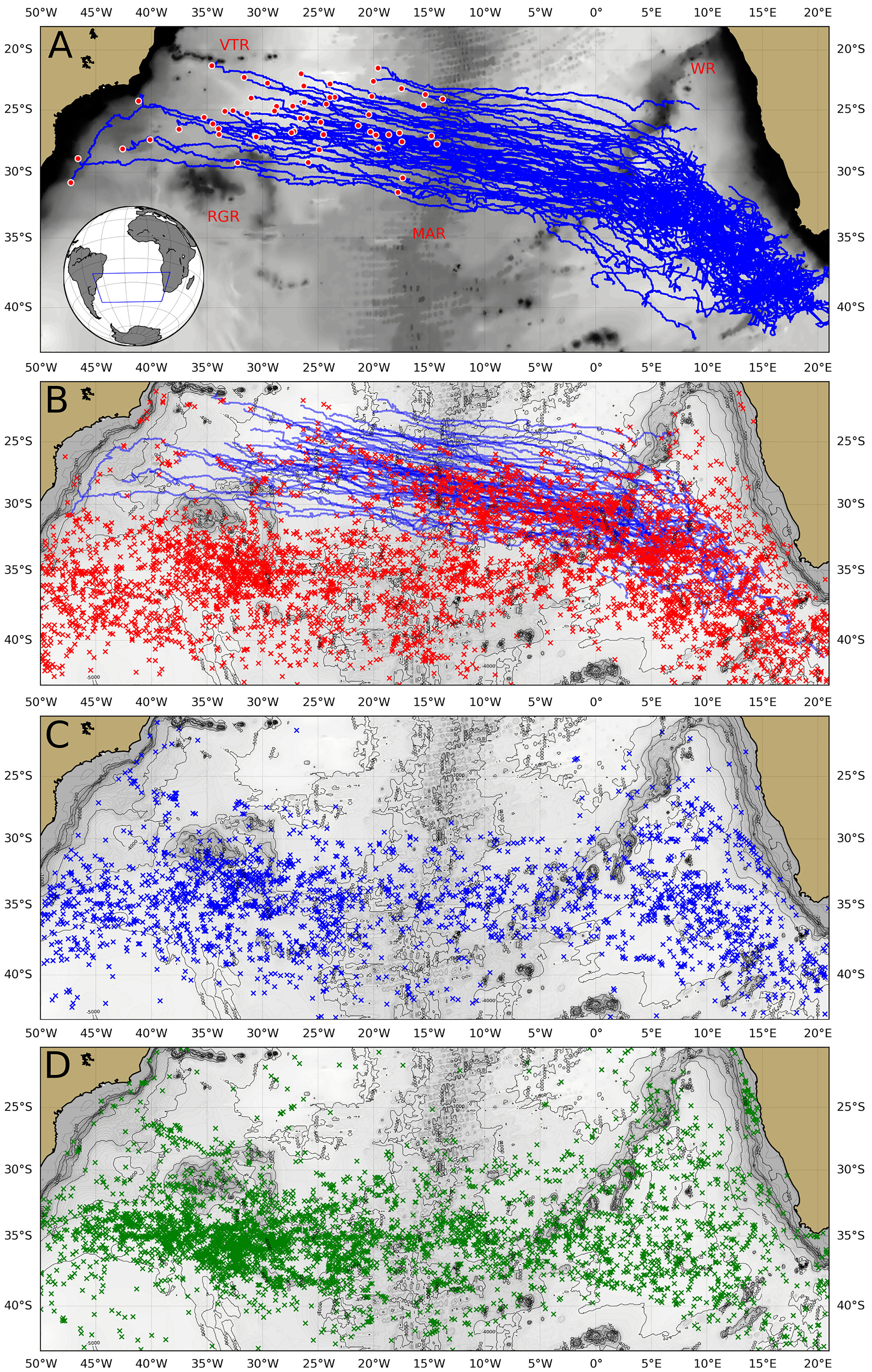
Figure 1 (A) Tracks of 56 long-lived Agulhas rings (blue lines) between 1993 and 2016 identified using an automatic algorithm. The set includes only the rings that reached the western basin. The acronyms WR, MAR, VTR, and RGR refer to Walvis Ridge, Mid-Atlantic Ridge, Vitória-Trindade Ridge, and Rio Grande Rise, respectively. The red circles mark the final tracking position of each ring. The bottom topography is shown in the background in gray. (B) Map with the paths of the Agulhas rings (blue lines) and the sites of detection of thermostads coincident with anticyclones (red x). (C) Map with the sites of detection of thermostads coincident with cyclones (blue x). (D) Map with the sites of detection of thermostads in profiles outside eddies (green x).
2.2 Temperature and salinity profiles
We sought profiles coincident in time with eddies. All profiles occurring within an area defined by twice the respective eddy radius were selected. Nevertheless, as mentioned, the eddy radius is an approximation, and it is not rare that the actual eddy does not fit a circular form. Thus, the chosen search radius aims to increase the chance of capturing coincident profiles close to the eddy edge (see Supplementary Figure 1).
We used the vertical profiles from the EN4.2.1 dataset (Good et al., 2013). The EN4.2.1 dataset includes eXpendable BathyThermograph (XBT) and Conductivity-Temperature-Depth (CTD) profiles from different cruises and programs (e.g., data from the XBT transects AX18 and AX97, provided by the NOAA/AOML High-Density Transects Program, and Argo profiles as well). Temperature and salinity profiles passed through an automatic analysis based on a quality control manual (U.S. Integrated Ocean Observing System, 2020).
2.3 Detecting mode waters
Temperature and salinity profiles were interpolated to a regular vertical interval of 5 meters using a piecewise cubic Hermite interpolating polynomial (Fritsch and Carlson, 1980). A difference criterion was applied to determine the mixed layer depth, defined as the depth where the temperature deviates by 0.5°C from the sea surface temperature (Foltz et al., 2003). Between the mixed layer depth and the 1,000 m depth, an automated algorithm identified layers defined by a threshold of vertical temperature gradient of 0.01°C/m (dθ/dz<0.01°C/m) (Provost et al., 1999; Sato and Polito, 2014). Only thermostads with temperatures in the range 18.0°C > t > 10.5°C, with a minimum thickness of 50 meters, and entirely inserted in the referred depth interval were considered. Afterward, each profile was visually inspected to guarantee that the thermostads were detected appropriately inside a ring (e.g., Supplementary Figure 1).
2.4 Rings properties
We used a two-layer model with reduced gravity to study the structure and dynamics of the Agulhas rings following Olson et al. (1985). In this model, a cylindrical coordinate system has its origin at the ring’s center, and the interface between the two layers with different densities (ρ1<ρ2) is approximately defined by an isotherm representing the main thermocline. Considering the high correlation between the sea surface height and the 10°C isotherm depth at the Agulhas Retroflection vicinities and along the rings’ corridor, this isotherm was used as a proxy for the thermocline (Olson and Evans, 1986; Garzoli et al., 1997).
The assessment of the volume and energy of the rings in the upper layer was performed using formulations derived from the model as follows:
where h1 is the depth of the thermocline within the ring, h∞ is the depth of the undisturbed thermocline in the far-field, A is the surface area of the ring, g′ is the reduced gravity, and v is the azimuthal velocity. Considering that the rings are frequently associated with other vortices that disturb the mass field in the actual ocean, we used the 10°C isotherm climatological mean depth from the World Ocean Atlas 2018 (WOA18) (Garcia et al., 2019). The azimuthal velocity (v) was calculated as the maximum of the average geostrophic speeds around the closed contours of sea surface height inside the ring, according to Chelton et al. (2011).
The reduced gravity that measures the restoring force and depends on local stratification was calculated according to:
where g=9.8 m/s2 is the gravitational acceleration, ρ1 and ρ2 are the mean potential density of the upper and lower layers calculated using temperature and salinity from the WOA18. The density integration in the lower layer was limited to 1,500 m depth or the ocean bottom when in shallow waters.
The instantaneous upper layer thickness in the center of the eddy was computed from the satellite sea level anomaly and the known mean thermocline depth and reduced gravity, using the following equation (Goni et al., 1996):
where is the mean upper layer thickness, equivalent to the thermocline depth at the far-field, η’ is the amplitude of the ring, that is the difference between the sea surface height in the center and at the border of the ring (Chelton et al., 2011), obtained from the altimetry, and B’ is the barotropic contribution to the sea surface level anomaly, where ' = 0, since |B'|≪|η'| .
Additionally, we calculated the upper layer thickness fitting a Gaussian function to the depth of the thermocline obtained at different distances from the ring center by temperature profiles, following Olson et al. (1985) and Goni et al. (1997):
where r is the radial distance measured from the center of the ring, assuming it is radially symmetrical, h0 is the maximum depth of the thermocline measured from h∞ at the ring’s center, and L is the ring radius. This method was used in two cases where at least five temperature profiles were synoptically available.
3 Results
We started exploring the occurrence of thermostads in the South Atlantic between the latitudes 20°S and 43°S from January 1993 through May 2016. The analysis included 99,167 profiles, of whom 10.4% (10,281) displayed thermostads. We found that 49.6% (49,186) of the profiles were collected within eddies, considering a search distance of twice the length of the radius centered on each eddy. When using a search distance of one eddy radius, we obtained percentages similar to Sato & Polito (2014), despite analyzing a more extended period and a dataset with three times the number of profiles. Most thermostad detections were inside vortices (62.8% of detections, or 6.5% of the profiles), with the number of occurrences in anticyclones being twice as many as in cyclones (see Supplementary Table 1).
Figure 1B shows the occurrence of thermostads within anticyclones (4,385). They extend along the parallel 35°S with concentrations west of 20°W and in the Cape Basin, east of 0°W. This pattern is roughly repeated for the thermostads within cyclones (Figure 1C) and thermostads outside eddies (Figure 1D). However, a distinctive characteristic is their spread along the eddy corridor depicted by the paths of long-lived Agulhas rings (Figure 1B). In contrast, regarding the thermostads in cyclones and thermostads outside eddies, there is a clear space along the corridor (Figures 1C, D). In the Cape Basin, there is a predominance of thermostads within anticyclones. While west of 20°W, thermostads outside vortices are more frequent.
The general picture emerging from this analysis is that the occurrence of thermostads inside anticyclones along the eddy corridor crossing the South Atlantic seems to be related to the translations of long-lived Agulhas rings. We will analyze this matter in detail below.
Our principal analysis focused on the 56 long-lived Agulhas rings tracked from the origin at the Cape Basin until the Brazil Basin between 1993-2016 (Figure 1A). The general characteristics of this subset of Agulhas rings are very similar to those presented by Guerra et al. (2018) for the original set of long-lived rings. The average lifetime of the 56 rings is 1,041 ± 213 days, and the average travel distance is 6,268 ± 1,286 km (mean ± standard deviation), including parent rings in case of merging and split-off events in the Cape Basin.
The interior of the Cape Basin is a well-known spot of turbulent mixing and stirring, where the anticyclonic Agulhas rings interact with topography, other anticyclones, and cyclones, resulting in dissipation, intensification, splitting, and merging events (see Boebel et al., 2003; Dencausse et al., 2010). Consequently, several short trajectories are crowded in the Cape Basin until the ring shows up as an isolated eddy ready to cross the Walvis Ridge (Figure 1A). The rings leave the Cape Basin after overcoming the Walvis Ridge (WR) and continue in a west-northwest course to eventually cross the Mid-Atlantic Ridge (MAR), in the case of long-lived ones. They reach the western basin in a latitudinal band, limited North by the Vitória-Trindade Ridge (VTR) and South by the Rio Grande Rise (RGR).
The number of identified coincident profiles with the Agulhas rings sums to 3,217 temperature profiles and 2,476 salinity profiles, produced by 741 XBT, 70 CTD, and 2,406 Argo profilers. The quality control rejected 141 temperature profiles and 282 salinity profiles. There is a corresponding temperature profile for every approved salinity profile in the qualified set. Figure 2, top panel, shows the number of coincident temperature profiles along the path of the 56 sampled Agulhas rings. The data reveal that roughly 75% of the coincident profiles occurred east of the Mid-Atlantic Ridge, while the other 25% sampled 38 rings in the western.
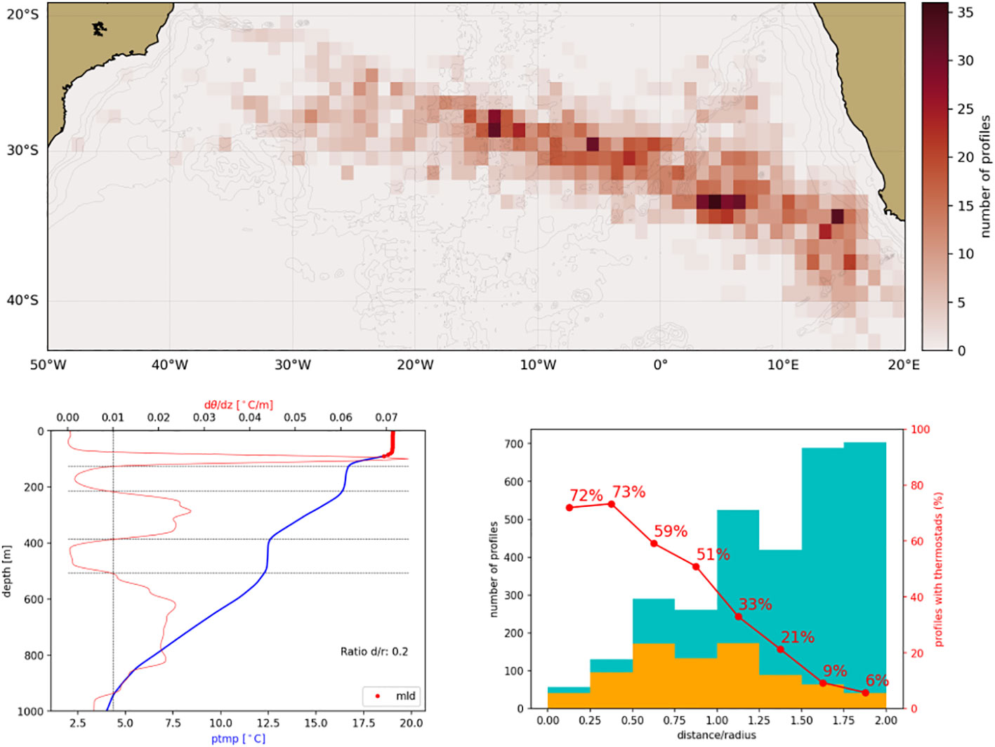
Figure 2 Temperature profiles inside Agulhas rings along the South Atlantic between 1993 and 2016. Top) Distribution of coincident temperature profiles and Agulhas rings, totaling 3,076 profiles, in a 1° x 1° resolution grid. The bottom topography is shown in the background in faded gray lines. Left) Temperature profile acquired within an Agulhas ring on the geographic coordinates 27.92°S of latitude and longitude 20.22°W, on 27-Jul-2006, close to the ring center (ratio distance/radius = 0.2). The red line indicates the vertical temperature gradient, and the red dots mark the mixed layer. The vertical dashed line marks the threshold for the vertical temperature gradient at 0.01°C/m. Right) The number of profiles acquired within Agulhas rings versus the ratio between the distance from the ring center and ring radius. Cyan: all the profiles; Orange: profiles with mode water signal. Red line: the percentage of profiles with detected thermostad in each class interval of distance.
Aiming to find signs of MW within the Agulhas rings, the set of coincident profiles was examined by an automated algorithm for thermostads searching, followed by a visual inspection. The search returned a total of 912 thermostads. Figure 2, left panel, illustrates a MW detection, presenting a temperature profile acquired within an Agulhas ring, in which we observe two thermostads: 16.5°C between 125-215 m, and 12.5°C between 385-505 m. As shown in the figure, when the vertical temperature gradient threshold is crossed, the limits of the layers are determined.
We examined the relationship between thermostads detection and profile distance from the ring center. Despite being detected throughout the entire range, from the center of the ring to twice the radius, it is noticeable that thermostads detection is relatively more frequent at a distance within a half-ring radius, where 73% of the profiles showed thermostads. As the distance from the center increases, the lesser the chances to detect them, as indicated by the decreasing percentage of profiles with MW towards the ring’s periphery (Figure 2, right panel).
Figure 3 shows a graphic summary of the classification of the Agulhas rings according to sampling and geographical distribution of MWs. Only 52 of the 56 long-lived Agulhas rings were sampled during the journey. We found the occurrence of thermostads in 46 rings, but only 38 of them were sampled in the western basin. Of those, 45% (17) had MW detected west of the Mid-Atlantic Ridge. On the other hand, 12 rings had MW detected during the life span but were not sampled on the western basin. Thus, for this specific subset, it is not possible to affirm that they were able to transport MW to the western basin. Half of the 34 rings sampled on the western side, with previous records of MW, did not show any signal west of the Mid-Atlantic Ridge. Thus, these figures should be considered with some caution due to the nature of the sampling. Besides, the mentioned 17 rings with no detected thermostads west of the Mid-Atlantic Ridge had four rings sampled a maximum of five times and whose profiles were undertaken at distances greater than one ring radius, which implies a lower probability of MW detection.
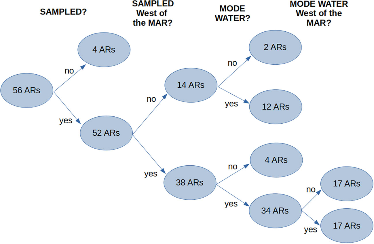
Figure 3 The Agulhas rings (ARs) classification according to sampling and presence of mode waters passed through a dichotomous tree. The 13°W meridian was used as a watershed for the South Atlantic, representing the Mid-Atlantic Ridge (MAR).
The temperature and salinity of the isopycnal layers showed bimodal distributions (Figure 4, top and right panels). A hypothesis test, applied separately for temperature and salinity, confirmed the difference between the two modes, with a p=0.0001. Then, we used the k-means method (Lloyd, 1982) to distinguish the two populations and determine their statistics, considering the pairs of temperature-salinity. The analysis evidenced two clusters of MW, which we named Type I (16.2 ± 0.6°C, 35.6 ± 0.1) and Type II (12.9 ± 0.7°C, 35.2 ± 0.1). The Type I MW is centered near the 26.2 isopycnal, and it is lighter than the Type II (centroid close to the 26.6 isopycnal). Figure 4, central panel, presents the clusters’ centroids (white circles) and the temperature-salinity pairs (triangles) corresponding to the pycnostads.
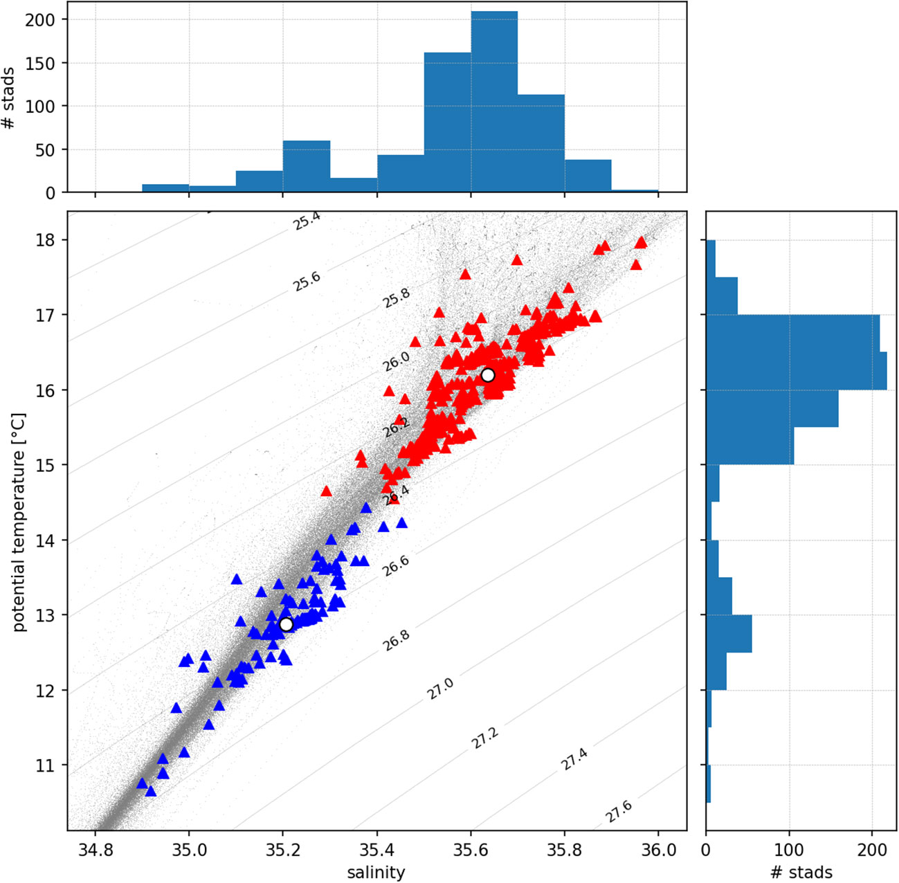
Figure 4 Temperature-salinity diagram including all qualified profiles acquired inside the rings (gray dots), and histograms of mean salinity (top) and mean temperature (right) of the pycnostads identified. The triangles show the t-s pairs of the pycnostads, and the white circles show the centroids of each mode water cluster (Type I in red and Type II in blue). The centroids have the following characteristics: Type I (16.2 ± 0.6°C, 35.6 ± 0.1 psu, 26.2 ± 0.1 σθ) and Type II (12.9 ± 0.7°C, 35.2 ± 0.1 psu, 26.6 ± 0.1 σθ).
The Type I MW was present in 45 rings, while Type II was in 32 rings. A total of 31 rings showed more than one variety of MW at least once during the lifetime. Only one ring studied in this work showed the isolated occurrence of Type II without the presence of Type I. When evaluating this single case, which is a ring sliced in a meridional section at position 27°S/9°W, we found remnants of a layer with the characteristics of Type I MW but already quite eroded.
Examining profiles with simultaneous occurrence of Type I and Type II MW in the environment outside eddies, we found 11 cases: five in the Cape Basin, three east of MAR, and three west of MAR. This subset represents 0.003% of the total number of profiles with detected thermostads outside eddies (3,820).
The spread of each type of MW trapped inside the rings is shown in Figure 5. Both types of MW were detected inside Agulhas rings from the southeastern region of the Cape Basin until the western basin at 34°W. They spread along the eddy corridor crossing the South Atlantic. Type I was more frequent than Type II, in general, as shown in the map and TS diagram (Figure 4), but the second was also detected at the westernmost recorded position. Type I was relatively more frequent westward from meridian 10°E.
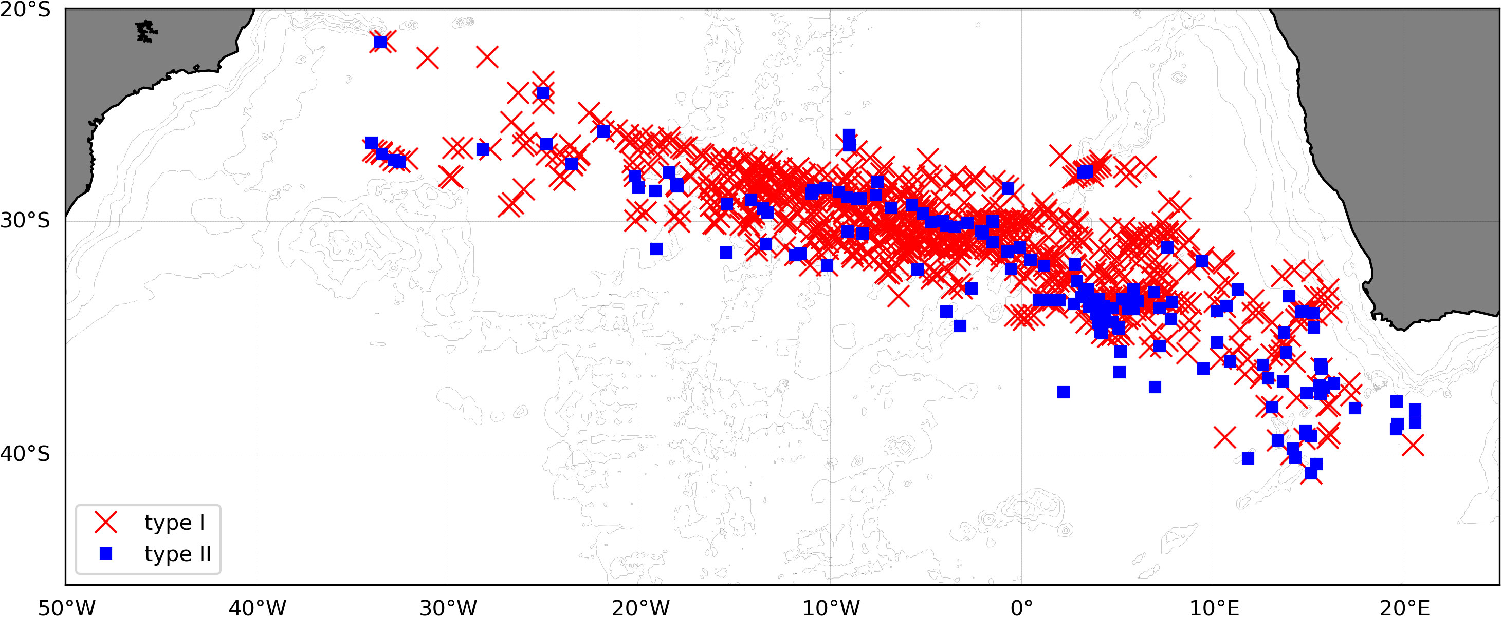
Figure 5 Map of occurrence of mode waters in Agulhas rings. Both mode water varieties were detected from the Cape Basin until the western basin. The bottom topography is shown in the background in faded gray lines.
We assumed the meridian 13°W as the watershed of the eastern and western basins, representing the Mid-Atlantic Ridge, to compare the characteristics of mode waters Type I and Type II on both sides of the South Atlantic Ocean. The total number of detections in the east is four times larger than in the west. Comparing the MW layers on both sides of the Atlantic, the maximum thicknesses for Type I and Type II are more prominent on the eastern, but there is no significant difference in the mean for the two types (295 m for both; see Supplementary Table 2). However, there is a significant increase in the depth of the core of Type I in the west. While on the eastern side, the average vertical distance between the two cores within the rings is 259 m, this space shrinks to 230 m on the opposite side. Ultimately, the temperature and salinity show no variation from the eastern to the western side, evidence that the water masses in the core of the rings may be preserved for time scales of years.
3.1 Particular cases: Three supersampled Agulhas rings
After a general description of the MW properties and spreading throughout the South Atlantic inside Agulhas rings, we will focus on three supersampled rings, whose MW characteristics and evolution were captured both in Lagrangian and in Eulerian sampling.
3.1.1 Ring Ana
The first ring, referred to as Ring Ana, was first detected at 38.26°S/17.10°E on 15-Aug-2004 and tracked until north of the Rio Grande Rise at 33°W, on 09-May-2007, in the western basin. Around longitude 7°W, the Argo float number WMO (World Meteorological Organization) 1900487 was captured by the ring and carried for more than 2,000 kilometers, performing 36 profilings inside the ring for 350 days (from 09-Nov-2005 to 25-Oct-2006). The trajectory of the advected Argo exhibits seven anticyclonic loops (Figure 6 - yellow triangles) between the eastern and the western side of the Mid-Atlantic Ridge. Two other Argo floats also profiled the ring, but for shorter times: WMO 1900525 (24-Oct-2005 to 21-Feb-2006) and WMO 1900285 (12-Mar-2006 to 31-May-2006).
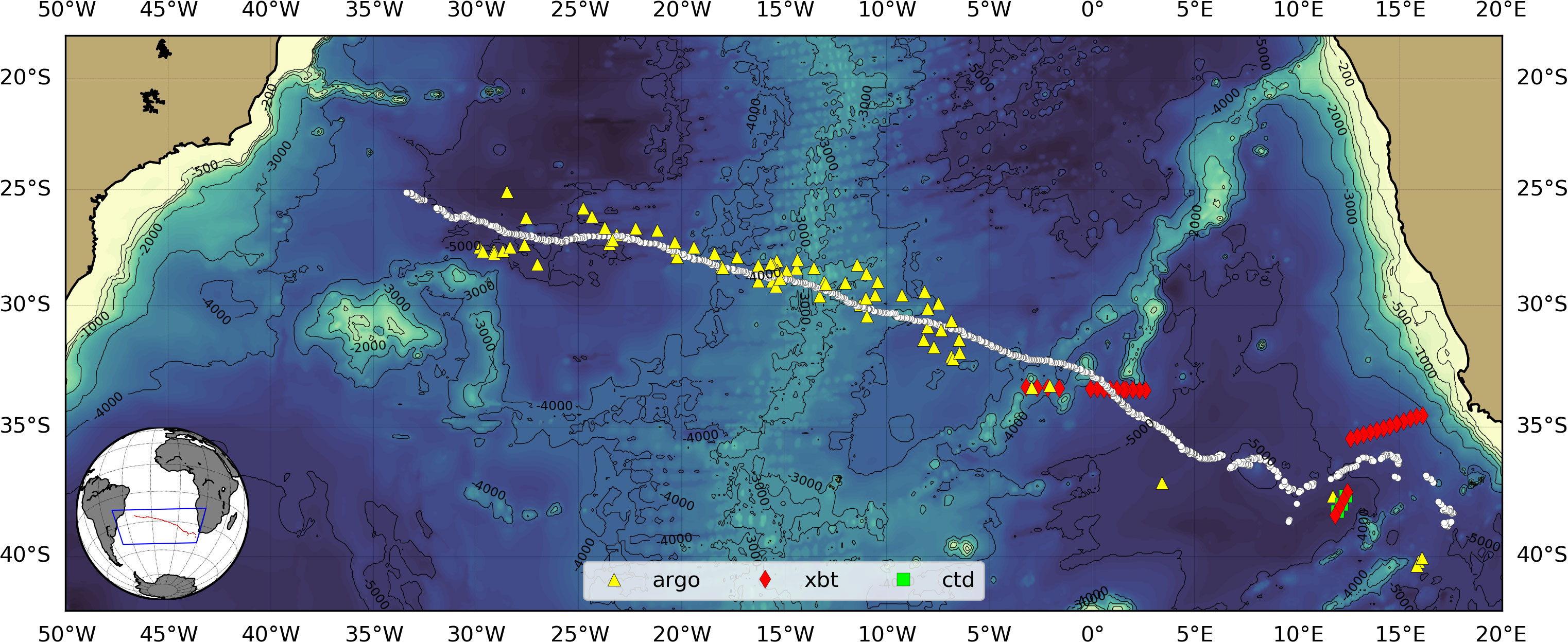
Figure 6 The path of the Ring Ana between 15-Aug-2004 and 09-May-2007 (white dots) and the locations of Argo (yellow), XBT (red diamonds), and CTD (green squares) profiles within the ring radius. The bottom topography is shown in the background.
The time evolution of the temperature and salinity vertical profiles made with the Argo 1900487 data showed two regions of the water column with low potential vorticity, with potential temperatures ranging between 16-17°C and 12-13°C, and their respective halostads of 35.6-35.7 and 35.1-35.2, between depths of 70-280 m and 400-550 m (Figure 7). They were classified as Type I and Type II MW, respectively, and they are present in this record only during the period the profiler was trapped inside the ring, as shown in Figure 7. The associated pycnostads for Type I and II were 1,026.1-1,026.2 kg/m³ and 1,026.6-1,026.7 kg/m³, respectively. The vertical dashed lines mark the period the Argo 1900487 was trapped (ratio distance/radius< 2). Before and after this period, it is possible to observe the surrounding stratification outside the ring, showing no thermostads or halostads in the same range of the properties of the two types of MW.
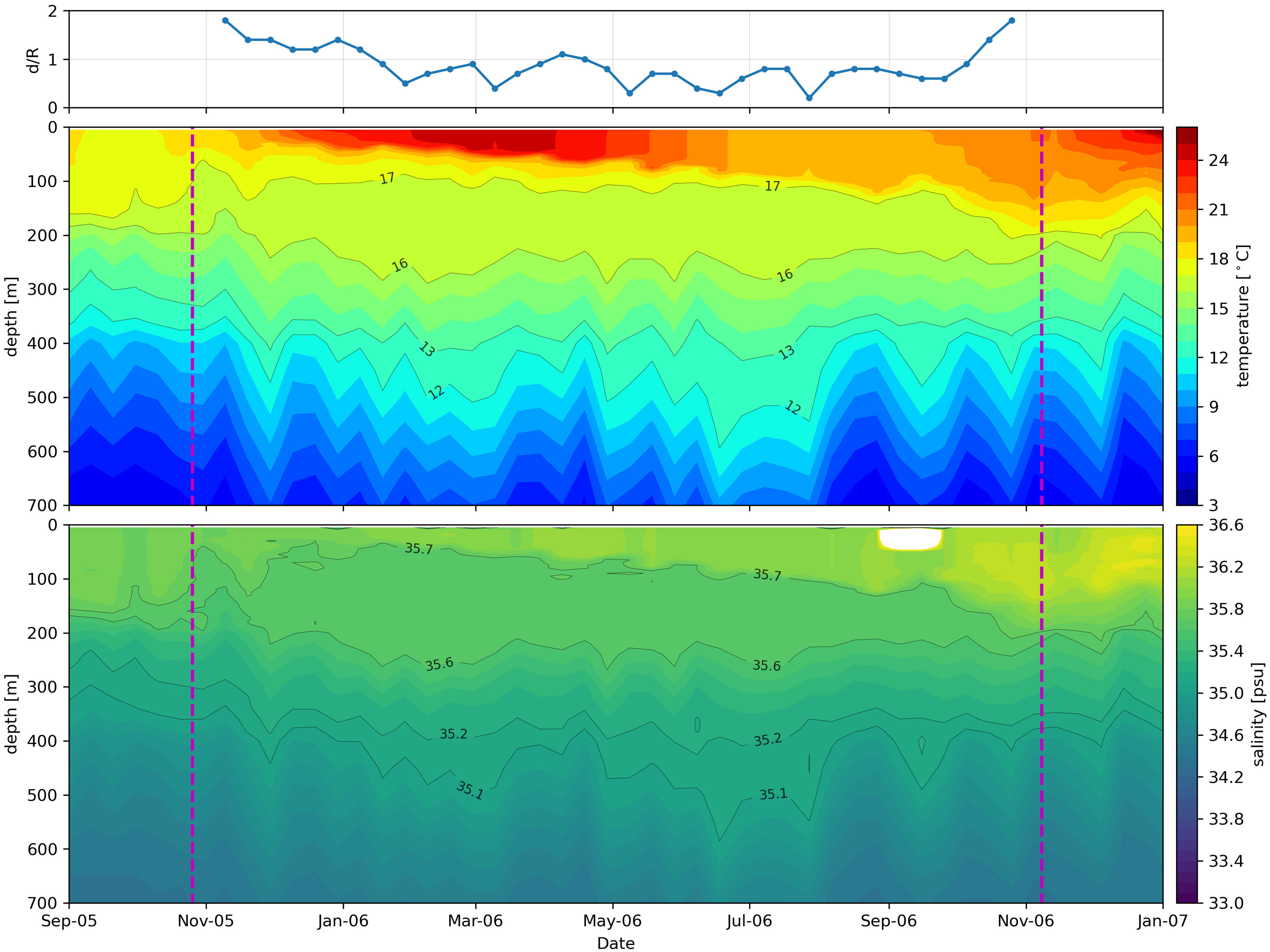
Figure 7 Temperature and salinity sections from Argo 1900487. Vertical dashed lines delimit the time the Argo remained inside the ring (from 09-Nov-2005 to 25-Oct-2006). It is possible to see two thick thermostads (16-17°C and 12-13°C) and halostads (35.6-35.7 and 35.1-35.2), classified as Type I and Type II. Top panel: the ratio between profile distance from the ring center and ring radius.
While Type I is noticed in the ring throughout the entire sampling duration, Type II is more evident during three periods only (February-March 2006, June-August 2006, and September 2006), when the profiling occurred closer to the ring’s center (d/r<1) (Figure 7, top panel). The thickness oscillation of the pycnostads suggests a lenticular shape of the MW layers, thicker as much closer to the ring’s center and thinner in its peripheral region. The profiler was entrapped during the austral spring and stayed sampling inside the ring until the following spring. The two other mentioned profilers (WMO 1900285 and WMO 1900525) confirm the temperature and salinity values (vertical profiles not shown) of the two MW at the same depth ranges. Despite the winter’s surface cooling, the recapture of the 16-17°C layer did not occur, evidencing the role of the ring in transporting MW away from the formation zone. The Argo data provide clear evidence that a well-defined front at the ring’s edge retains the MW in its interior core as the Argo profiles acquired outside the ring exhibit no signal of them. These Lagrangian observations provided by the Argo profilers unequivocally evidenced that MW can be preserved within the Agulhas rings for long distances.
Just before Ring Ana leaves the Cape Basin (near the Greenwich meridian), it was sampled by XBT probes from an AX18 cruise on 25-26-May-2005 (Figure 8, left panel). Even though the Type I MW was present trapped inside the ring five months later (Figure 7), the temperature profiles in May show alternatively a presence of a well-developed 12°C thermostad (classified as Type II) with 300 m thickness and a surface signal of the 17°C (Figure 8, right panel) associated with the local mixed layer. These results suggest that the formation of the Type I MW may occur even on the verge of the ring leaving Cape Basin and translating to the ocean interior. Unfortunately, the analyzed data could not capture the subduction of Type I, and it is hypothesized that the MW formation had occurred in the interval between the sampling events.
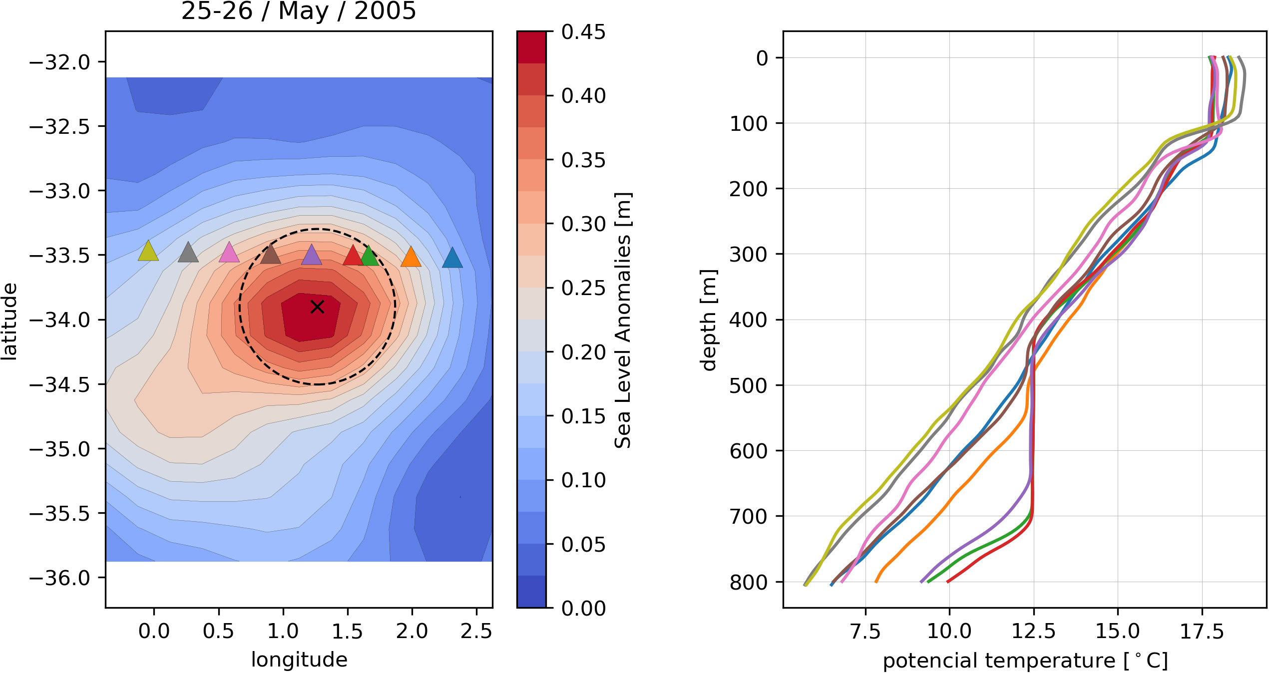
Figure 8 Left panel: Altimetry map showing the Ring Ana just before leaving Cape Basin and XBT launches in a section crossing it towards the west. The dashed circle marks the radius of the ring, estimated at 67 km. Right panel: Temperature profiles from the XBT section. The profile colors identify the deployments.
3.1.2 Ring Eliza
The second ring, referred to as Ring Eliza, results from a split-off occurring approximately on position 38°S/16°E from a ring shed from the retroflection on 01-Aug-2007, just one month before the split-off. It was tracked for 1,007 days from the shedding until its demise in the western basin near 29°W on 04-May-2010 (Figure 9).
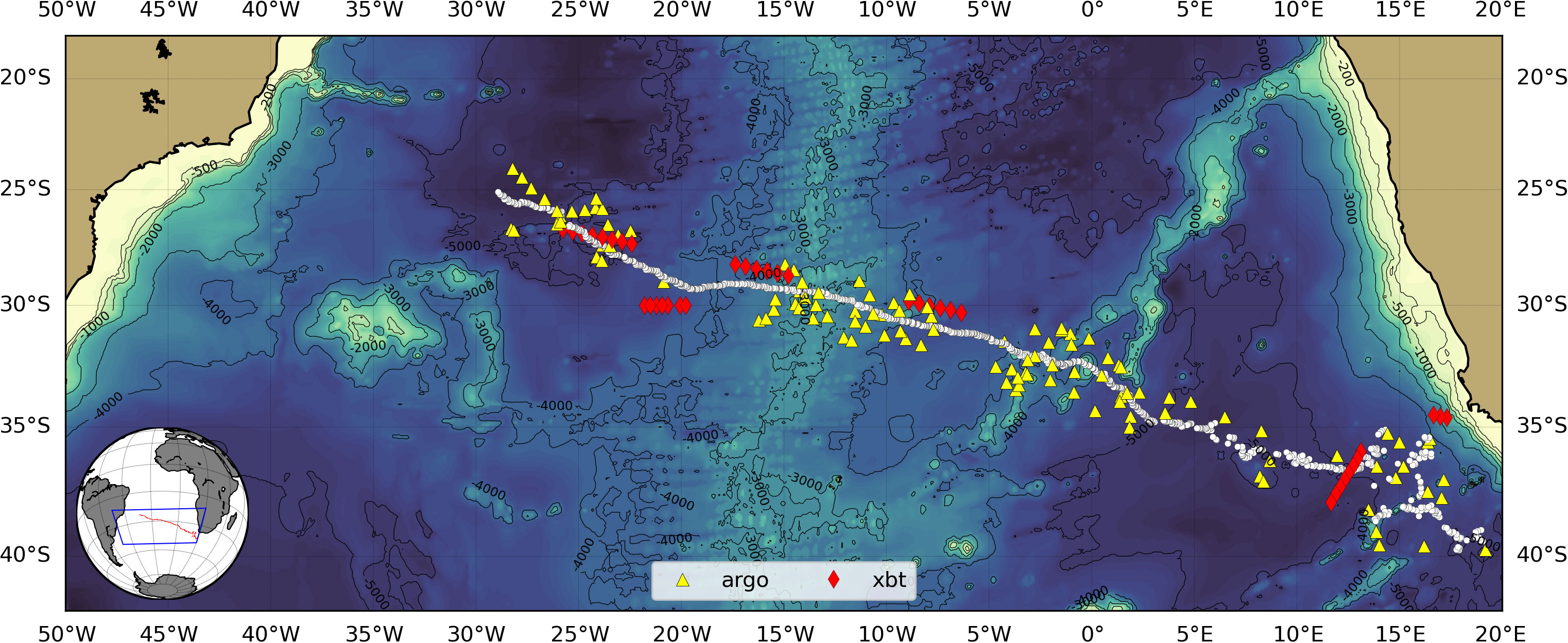
Figure 9 The path of the Ring Eliza between 01-Aug-2007 and 04-May-2010 (white dots) and the locations of Argo (yellow) and XBT (red diamonds) profiles within the ring radius. The bottom topography is shown in the background.
Along its path, the ring was sampled on different occasions but remarkably at longitudes 8°W, 16°W, and 24°W, by three consecutive AX18 cruises in February and July 2009 and January 2010, respectively, when it was sliced. During the cruises, XBT probes were deployed every 50 km, reaching a depth of 850 m. The temperature sections illustrate the vertical structure of the ring in distinct moments of its evolution (Figure 10). On all three occasions, the data showed a large volume of Type I MW (16.4°C) inside the ring, with a thickness of approximately 200 m, evidencing the lenticular structure of the imprisoned water.
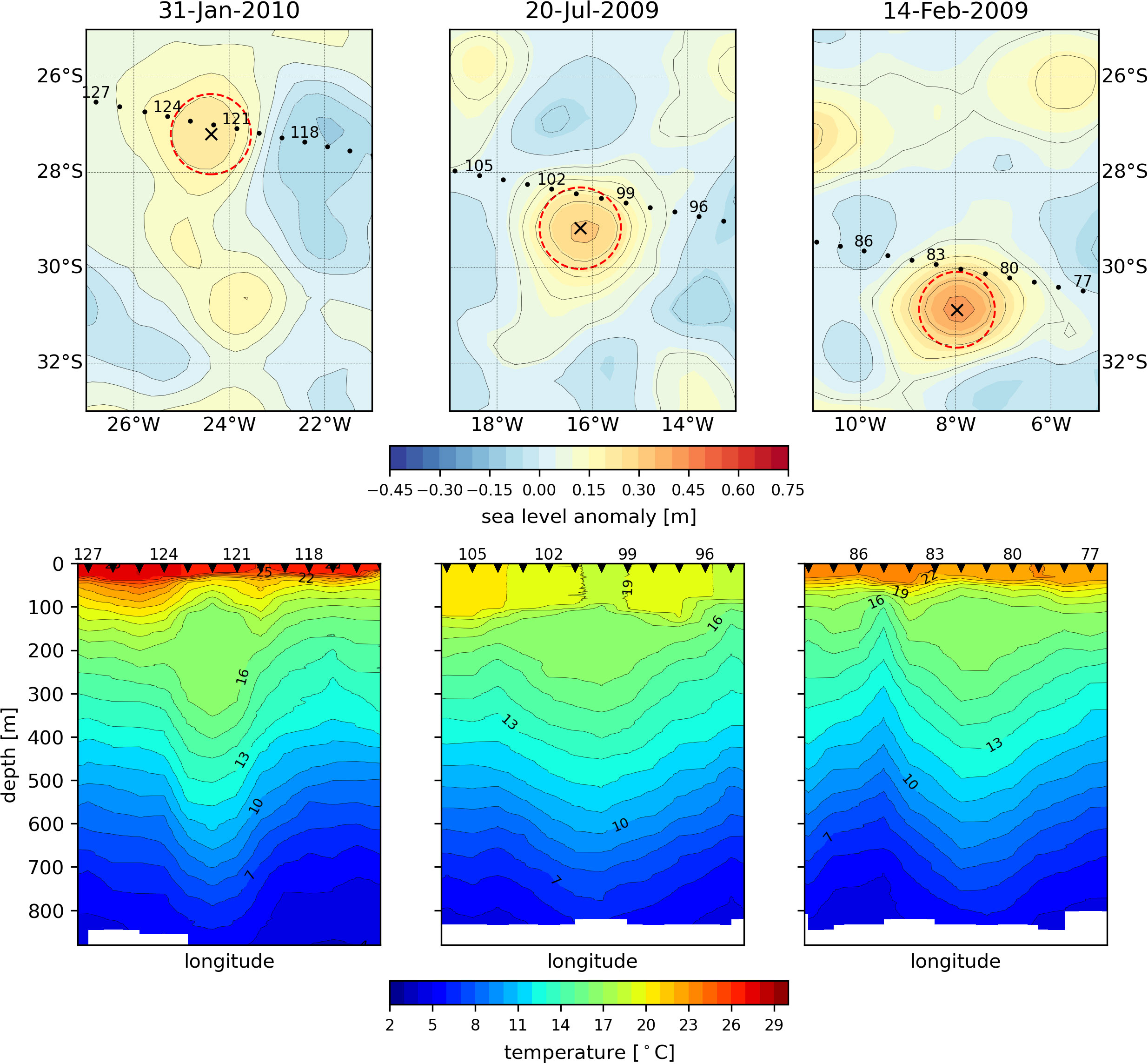
Figure 10 Three temperature sections were sampled across the Ring Eliza in successive AX18 cruises in February 2009, July 2009, and January 2019. The top panels show altimetric maps of the ring with numbered deployment stations. The red circle delimits the area defined by one ring radius (93 km, 95 km, and 88 km, from older to younger). The bottom panels show the three temperature sections.
The first section was sampled in February 2009 before the ring crossed the Mid-Atlantic Ridge, while the second, in July 2009, was just after. We could find no signs of any possible influence of the ridge on the ring’s structure after its passage. In January 2010, the section sliced the ring closer to the center. On that occasion, the thermocline depth inside the Ring Eliza, represented by the 10°C isotherm, was 150 m below its undisturbed depth outside the ring. The thickness of the lenticular-shaped MW was approximately 250 m near the center of the ring. Like what was observed on Ring Ana, the surrounding waters outside Ring Eliza showed no thermostads in the same depth range.
Between 25°W and 29°W, Ring Eliza was sampled 13 times by three Argo floats until its demise (Figure 9). Four profiles confirmed the presence of a 115 m thickness pycnostad with a temperature of 16.4°C and a salinity of 35.7. The surface signal of the ring was faint past 29°W, and the tracking algorithm could not continuously follow its trajectory except for short periods. Instead, a positive sea level anomaly was going west at the same speed as the ring but not as a coherent eddy. We decided to follow it visually and search for profiles nearby. We could find eleven profiles produced by four Argo floats (Figure 11, left panel). Despite the altimetric signature of the ring as a coherent feature weakening since 29°W, which could indicate the dismantling of the ring, the Argo profiles showed the persistence of the previously detected thermostad with temperature centered at 16.4°C (Figure 11, right panel) and salinity of 35.7 (not shown) until reaching the meridian 38°W, approaching the continental slope region dominated by the southward flow of the Brazil Current.
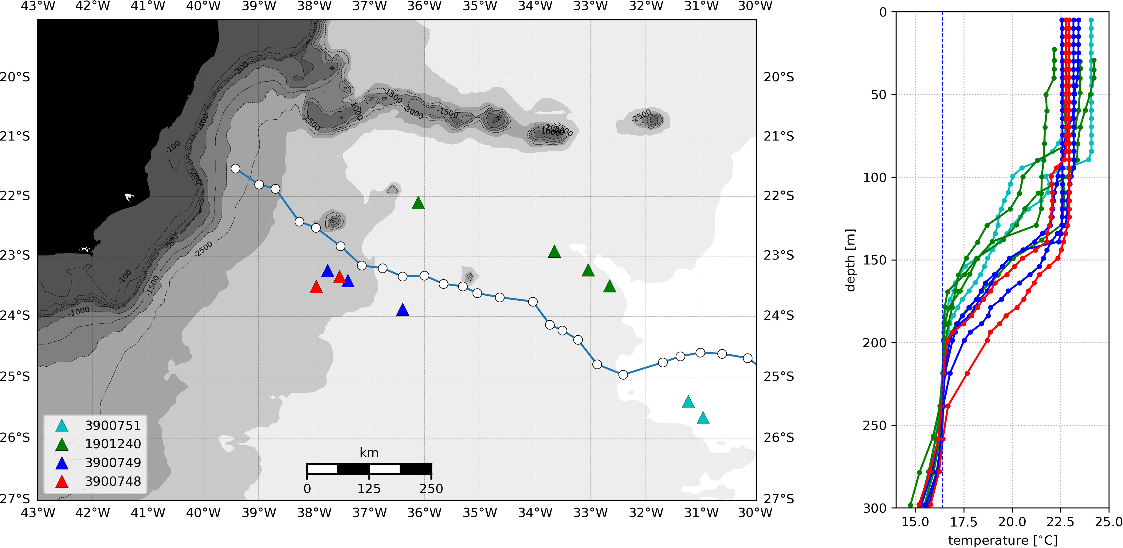
Figure 11 Trajectory of the sea level anomaly related to the Ring Eliza between 30°W and the Brazilian coast at 39°W (18-May-2010 through 02-Nov-2010). Left: Triangles mark the positions of the Argo floats that sampled the Type I mode water within a radius of 150 km from the center of the feature. The bottom topography is shown in the background in gray. Right: Temperature profiles measured by the Argo floats. The vertical dashed blue line marks the thermostad temperature at 16.4°C.
3.1.3 Ring Jeannette
The track of the ring referred to as Ring Jeannette begins on 28-Jan-2012 at 39°S/17°E and finishes on 27-Dec-2015 at 21°S/35°W, at the southern flank of the Vitória-Trindade Ridge, Brazilian coast (Figure 12).
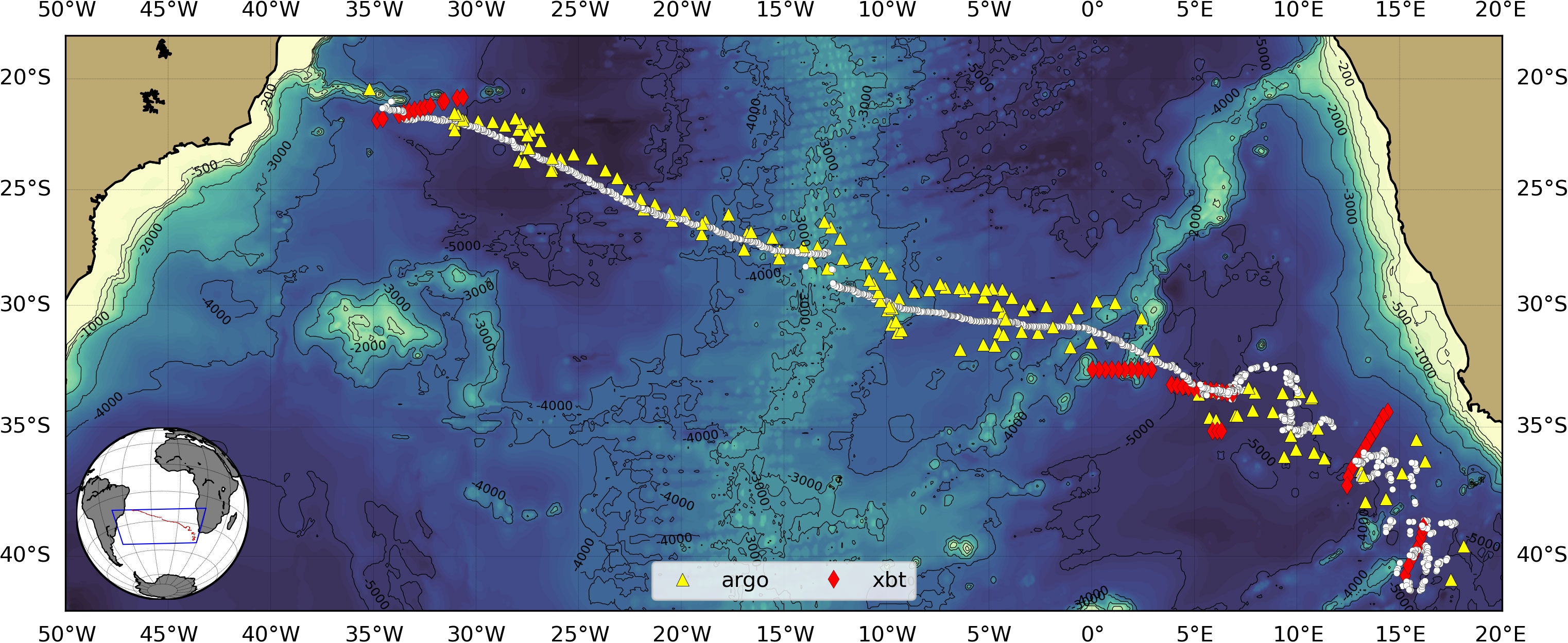
Figure 12 The path of the Ring Jeannette between 28-Jan-2012 and 27-Dec-2015. Besides the Argo profiles distributed along its route through the Atlantic, two XBT sections crossed the ring, one in the Cape Basin and the other next to the Brazilian coast. The bottom topography is shown in the background.
Ring Jeannette is one of those thirty-ones observed rings that carried both types of mode water. Two XBT sections crossed the ring, the first in the Cape Basin and the other next to the Brazilian coast just before its demise. The temperature sections clearly show the two thermostads on both occasions (Figure 13). The temperature shift in the thermostads is more pronounced in the shallow one. While its mean temperature was 15.6°C in the Cape Basin, and two and half years after, close to the Brazilian coast, it was 16.3°C, the deep thermostad conserved 13.8°C on both sides of the Atlantic. However, examining the Argo profiles between the two XBT sections, we observed that the shifting occurred possibly at the passage through the Walvis Ridge. Previous studies reported the role of the Walvis Ridge on the transformation of Agulhas rings due to volume exchanges with the environment (Richardson, 2007; Nencioli et al., 2018). Furthermore, the thicknesses of the thermostads are roughly two times larger in the Cape Basin. The vertical extension was shrunk with the aging of the ring, as previously observed in Agulhas rings by other studies (Guerra et al., 2018; Nencioli et al., 2018), evidencing its erosion.
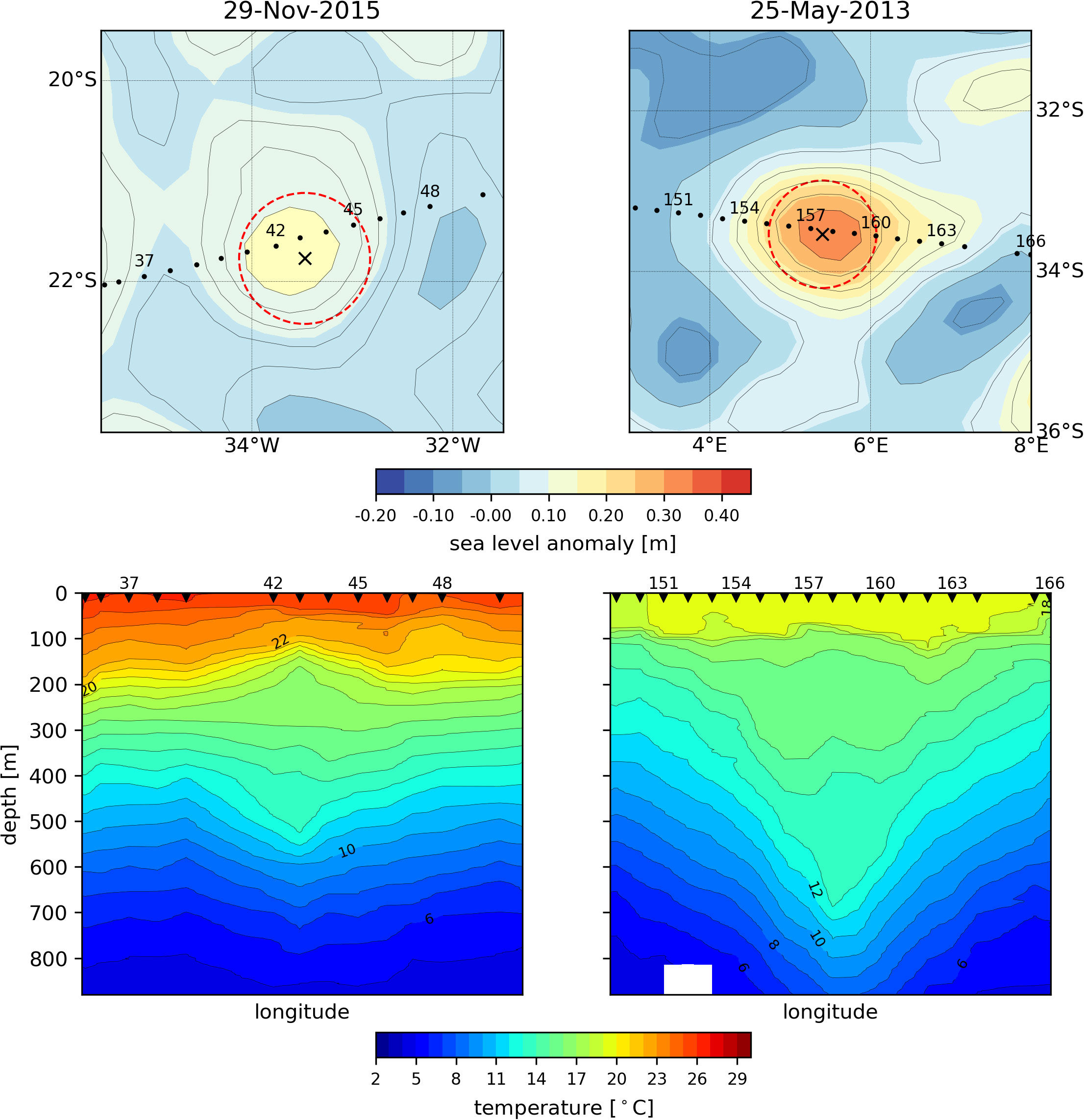
Figure 13 Temperature sections were sampled across the Ring Jeannette in the Cape Basin (right) and next to the Brazilian coast (left) in May 2013 and November 2015. The top panels show altimetric maps with numbered XBT deployments. The red circle delimits the area defined by one ring radius (72 km in Nov/2015 and 74 km in May/2013). The bottom panels show the temperature sections.
The ring that propagated along the track shown in Figure 12, and that we named Ring Jeannette, was also studied by Nencioli et al. (2018). However, the authors followed it in two steps. They reported a spawning of a ring, called B12, from the merging of two Agulhas rings at the Mid-Atlantic Ridge. The seminal rings were formed in the Cape Basin and translated to the west in parallel tracks until the encounter. They called the north track AN1 and the south AS2. The entire track of our Ring Jeannette comprises Nencioli’s south track AS2 and B12. A possible interpretation for this distinction is that our tracking algorithm, in the case of merging, continues the track of the nearest eddy from the previous time step (for details, see Guerra et al., 2018).
We examined the profiles coincident with the north track (AN1), including an XBT section crossing the ring, and observed only the shallow thermostad (Type I). Nevertheless, the analysis of the southern track (AS2), coincident with our track, revealed the presence of both Type I and Type II MW. Our findings are consistent with Nencioli’s results showing the southern track (AS2) as the main contributor to the B12. An interesting side finding was that after a merging event, it is possible to identify water masses from the core of the seminal vortices in the newborn vortical feature.
4 Discussion
The Cape Basin receives warm subtropical waters from the Agulhas Retroflection and intense subpolar winds (Gordon, 1985; Gordon et al., 1987). The air-sea fluxes in the region exceed any other in the Southern Hemisphere (Bunker, 1988; Walker & Mey, 1988). Under these conditions, MWs are produced with potential temperatures of 17.4-17.8°C, and those most weathered with temperatures of ~16.5°C, predominantly found around Agulhas Retroflection but also trapped in Agulhas rings, as discussed in the literature (e.g., Olson et al., 1992). The occurrence of deep 17°C mixed layers in the late winter in the Cape Basin is confirmed by several Argo and XBT profiles analyzed in this study (see Figure 8 and Supplementary Figures 2, 3). Figure 14 shows the WOA18 sea surface temperature for September, at the end of the austral winter, in the Southeastern Atlantic Ocean. In the Cape Basin, the average surface temperature is lower than 17°C, while temperatures are higher in the adjacent Angola Basin and Agulhas Retroflection region. The analysis of the trajectories of the three supersampled rings (Ana, Eliza, and Jeannette) reveals that while in the Cape Basin, they experienced two consecutive winters in the region of occurrence of temperatures associated with the Type I MW. The stars in the figure show the positions of the rings in September. The general picture emerging from the analysis is that the Type I MW is formed in the Cape Basin, a region with the necessary conditions to produce it, rather than a modified SIMW. This finding is congruent with the works of Capuano et al. (2018) and Laxenaire et al. (2019), who claimed that the 16-17°C STMW found within Agulhas rings is, in fact, the Agulhas Ring Mode Water (ARMW).
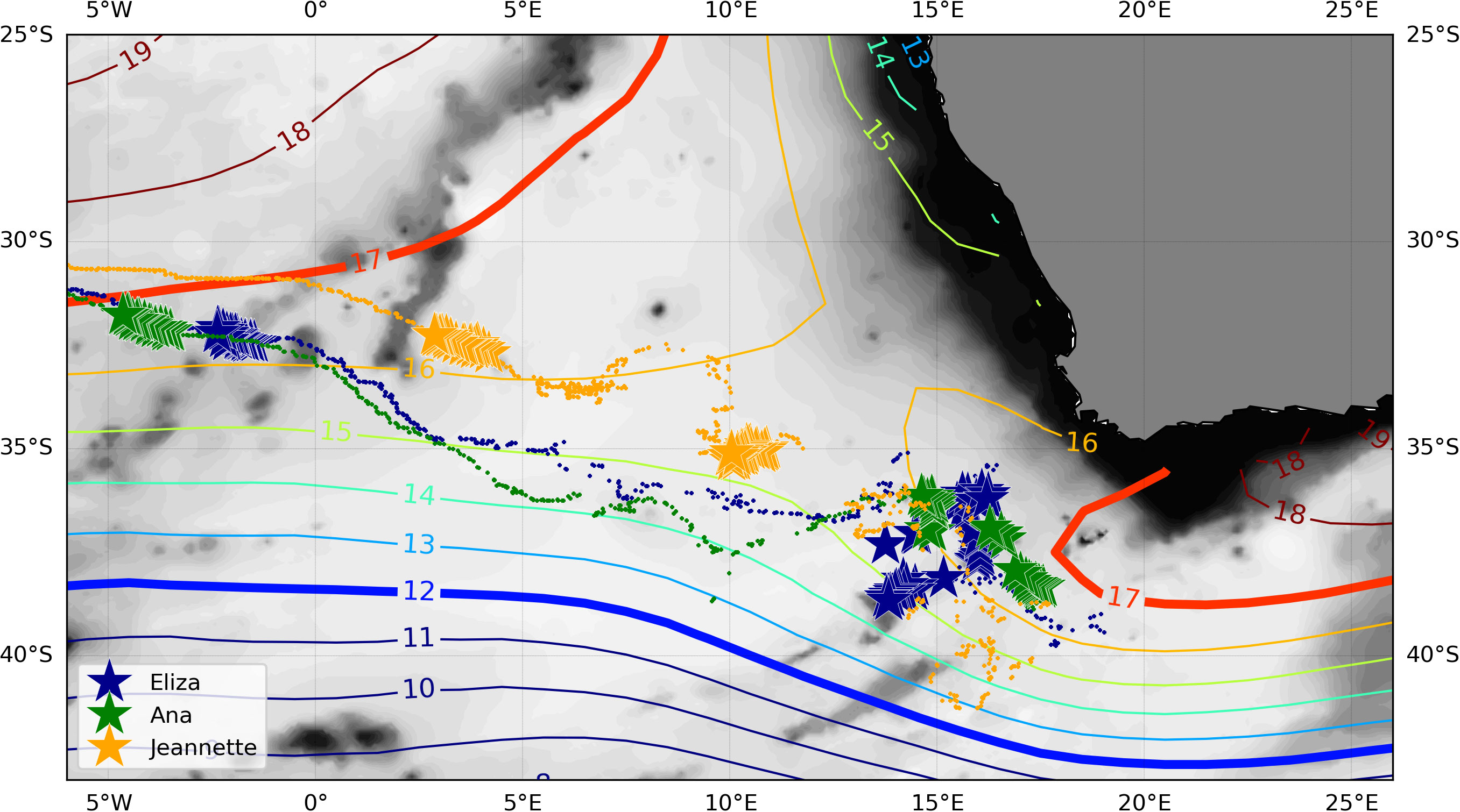
Figure 14 Mean sea surface temperature, in degrees Celsius, for the Cape Basin in September (WOA18). The trajectories of the three supersampled rings are plotted over the map. The stars mark the positions of the rings in September, the end of the austral winter. The bottom topography is shown in the background in gray.
The Type II MW, characterized by a deeper 12°C thermostad, was also observed inside Agulhas rings, as shown in detail for rings Ana and Jeannette. Some papers have documented such occurrences and earlier attempts to identify their origin (McCartney, 1977; McCartney & Woodgate-Jones, 1991). Previous research has supported the hypothesis that the 12°C thermostad would be a variety of South Indian Ocean Subantarctic Mode Water (SAMW) (McDonagh and Heywood, 1999). Other authors have argued that it results from entraining cold low-salinity Subantarctic Surface Water injected from south to north in the retroflection region as a wedge during the ring-spawning process (Gordon et al., 1987; Lutjeharms and van Ballegooyen, 1988). The high levels of oxygen of this alleged local variety of SAMW provide convincing evidence in favor of a possible origin directly from wintered surface waters from the south of the Subtropical Front, close to the Retroflection, instead of being derived from the Indian Ocean via leakage (Gordon et al., 1987; Arhan et al., 1999; Schmid et al., 2003). Gladyshev et al. (2008), after a detailed analysis of transect data from South Africa until the southern limit of the Antarctic Circumpolar Current, crossing three Agulhas rings, showed that both ways are possible.
More recently, Chen et al. (2022) proposed a redefinition of the three STMWs discussed by Sato and Polito (2014). They reasoned that only one variety originates from the Brazil Current recirculation, whereas the other two develops into the Cape Basin under the influence of the Agulhas leakage. Our Type I MW relates to the most saline variety (SASTMW2), and the Type II MW to the densest variety (SASTMW3). Corroborating the conclusions of McDonagh and Heywood (1999); Chen et al. (2022) demonstrated that, contrary to the findings of Smythe-Wright et al. (1996), a ring in the southeast Atlantic carrying MW with a potential temperature of 13°C and salinity of 35.2 psu originated at the Agulhas Retroflection and not at the Brazil-Malvinas Confluence as initially supposed, corroborating the conclusions of McDonagh and Heywood (1999). Whether the 12-13°C thermostad, by origin, is subantarctic or subtropical, from a remote site in the South Indian Ocean, or locally formed, remains controversial and deserves more research.
Each Agulhas ring is unique, having its characteristics related to its formation, depending on the staying period in the Cape Basin, the intensity of air-sea fluxes, and interactions with other eddies (e.g., Arhan et al., 1999). Several studies reported the occurrence of rings with or without thermostads (van Ballegooyen et al., 1994; McDonagh et al., 1999; Arhan et al., 1999; Garzoli et al., 1999). As shown in Figure 14, the three rings (Ana, Eliza, and Jeannette) had similar trajectories, approached the climatological position of the surface 12°C isotherm, and remained at least two winters east of the Walvis Ridge, but in different years. Unlike rings Ana and Jeannette, the Ring Eliza did not show the Type II MW in any vertical profile, inside or outside the Cape Basin. This result might indicate that this MW was not available during the ring formation. Thirteen other rings analyzed in the present study also contained the Type I MW exclusively.
Conversely, our data show that 31 distinct rings presented Type I and Type II MW during their life span, detected simultaneously or not. That was the most frequently observed situation (67% of the 46 rings with detected thermostads). The causes for some rings having only the Type I MW and others doing both types are still unclear. It is noteworthy that only one ring showed the isolated occurrence of Type II without the presence of Type I.
From the beginning of systematic satellite altimetry with the Geosat until nowadays’ multi-satellite altimetry, some decay curves for Agulhas rings have been proposed, all showing the exponential decline of amplitude along the trajectory (Gordon & Haxby, 1990; Byrne et al., 1995; Schouten et al., 2000; Guerra et al., 2018). The decay curves suggest that most rings disintegrate and diffuse their content within the subtropical gyre. Byrne et al. (1995) argued that mode water volume decays with distance from the formation zone at the same rate as the ring’s sea surface height. However, rings’ structure and hydrography variations while they cross the South Atlantic Ocean are barely known. Our results demonstrate that Agulhas rings can advect mode waters for long distances throughout the South Atlantic Ocean, reaching distances superior to 4,000 km until the western basin. This reinforces the idea that Agulhas rings are essential to the ventilation of the South Atlantic thermocline with relatively warm and saline waters, not restricted to the eastern sector of the subtropical gyre. Regarding the decay rate of the mode water content, the sampling provided by Argo profilers is insufficient to solve this puzzle. Hypothetically, a time series of the thermocline depth at the ring’s center would be necessary to illustrate the erosion of its core. Although Ring Ana has been continuously sampled for more than one year by Argo profilers, it is impossible to confirm the hypothesis since it occurred at different positions relative to the ring’s center and sparsely in time. Oscillations of the thermostads thicknesses associated with profile distance to the ring center (Figure 7) suggest a lenticular shape of the isopycnal layers, but nothing to state about volume.
In the case of Ring Eliza, a serendipitous coincidence of three sequential cruises and the ring trajectory within one year produced slices that reveal its internal structure while crossing the subtropical gyre. Ring Jeannette was also surveyed on two cruises lagged by two and a half years, being the first just before the ring leaves the Cape Basin and the last next to the Vitória-Trindade Ridge. Table 1 presents the volume and energetics of the rings Eliza and Jeannette and the parameters used in the reduced gravity model, calculated as described in Section 2.4.
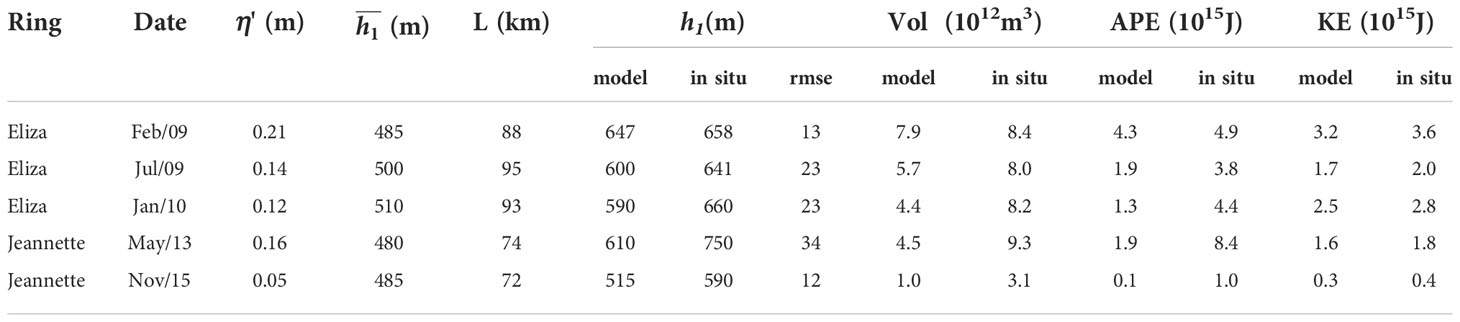
Table 1 Parameters used in the two-layer model with reduced gravity. The values of were obtained from the WOA18 climatology, while η' and L came from the altimetric map. The depth h1 at the center of the ring, Volume, Available Potential Energy, and Kinetic Energy were calculated from the model and from the in situ data for rings Eliza and Jeannette.
The amplitude and radius of the rings were determined from the altimetry. The mean upper layer thickness, , was obtained from WOA18 climatology. The instantaneous upper layer thickness, h1, was calculated using altimetry and verified with the in situ data. The radial distribution of profiles along the rings’ sections made a Gaussian curve fitting possible to determine the thermocline depth within the rings, even if the section had not crossed its center. The root mean squared error (rmse) expresses the difference between the thermocline depth measured by each profile and the value from the Gaussian fitting (i.e., how well the curve fits the data). The derived Volume, APE and KE, were computed from the h1 estimated by the two methods. Using in situ data, we could then examine the time evolution of the ring’s characteristics (Volume, APE, and KE) and assess the uncertainties of estimates based exclusively on altimetry data.
Olson et al. (1985) remind us that a simple diagnosis of eddy evolution could be made by assessing its volume. The decay curves are generally time functions of eddies’ amplitude obtained from satellite altimetry. The high correlation between the sea surface height and thermocline depth turns possible to assess the eddies’ volume. However, the analysis of the rings Eliza and Jeannette using synoptic in situ measurements revealed significant differences from satellite estimates (see Table 1). The volume calculated using temperature profiles for Ring Eliza was 6%, 40%, and 86% larger than the satellite estimates. The same was observed for Ring Jeannette with 107% and 210%. The difference is because the observed thermocline within the rings is deeper than the estimated with the altimetry.
Regarding the APE, the difference between the values calculated from the altimetry for both rings and the mean values presented by Guerra et al. (2018) for the Agulhas rings along the Atlantic is not significant. Nevertheless, the APE values calculated with in situ data show a significant increase since the difference between the thermocline depth within the ring and its undisturbed mean is squared. On the other hand, the KE values present an average increase of just 17%.
The numbers indicate that the usual estimates based on satellite altimetry could be overrated regarding the decay rate. The volume of Ring Eliza estimated with altimetric data reduced by 44% between February 2009 and January 2010, while the calculated with in situ data decreased by 2%. The analysis of Ring Jeannette displayed a distinct scenario where the variation of satellite estimates and in situ data converge. Between May 2013 and November 2015, its altimetric volume reduced by 78% and 67% for the in situ. At least for Ring Eliza, there was a negligible mass loss in the studied interval, despite the decay indicated by the altimetry. The results provide preliminary evidence that the rings’ decay rate based on satellite altimetry might not be an accurate measure to evaluate their life span and, ultimately, their impact on circulation.
A remarkable fact about the Ring Eliza is its sinking and consequent loss of coherence on the surface. As Laxenaire et al. (2019) observed, a reduction in the eddy surface intensity may not necessarily be associated with its dissipation but with its subsidence. Future studies will have to investigate further why some rings do not fit the model estimate.
In addition, the thermostads within anticyclones west of 20°W and north of 30°S might be related to Agulhas rings even if apparently without connection with the trajectories depicted in Figure 1B (blue lines). We tracked the Agulhas rings that left the Cape Basin without considering splitting or merging during their journey. Nevertheless, Laxenaire et al. (2018) developed an interesting concept of a network of Agulhas rings that included the seminal rings (122 trajectories) and their descendants resulting from splitting and merging, linking impressive 730,481 eddies into 6,363 segments over 24 years of satellite altimetry. Therefore, it is probable that those anticyclones were Agulhas rings’ descendants not followed by our algorithm or Agulhas rings that had lost the surface signal but followed existing in the subsurface, just like the super-sampled Ring Eliza.
5 Conclusions
This work analyzed temperature and salinity profiles collocated with 52 long-lived Agulhas rings between 1993 and 2016. We found that 88% (46/52) of the rings carried mode waters. Our results demonstrate that the Agulhas rings can advect mode waters for long distances through the South Atlantic Ocean, crossing the MAR and reaching the western basin, where 45% (17/38) of the rings sampled still carried significant amounts of mode waters. Most long-lived Agulhas rings disappear on the altimetric maps when they reach 30-40°W, where they may dissipate or coalesce with other vortices. Nevertheless, we present new in situ evidence that rings may lose surface signature and continue moving westward below the surface, marked by the low potential vorticity of the mode water core and possibly interacting with the Brazil Current system.
Two types of mode waters were determined in the range 16.2 ± 0.6°C, 35.6 ± 0.1 (Type I) and 12.9 ± 0.7°C, 35.2 ± 0.1 (Type II). Their spread along the eddy corridor crossing the South Atlantic defines a positive anomaly in temperature and salinity, supporting the concept that the Agulhas rings have an essential role in the ventilation of the South Atlantic thermocline not restricted to the eastern sector of the subtropical gyre. The necessary conditions to form the Type I MW can be found in the Cape Basin. Field data show a ring with a well-developed Type II thermostad and an outcropped Type I. Both mode waters were present inside that ring five months later and continued being sampled for one year while crossing the Atlantic.
The occurrence of rings with both Types I and II MW was most frequent (67%). The analysis of three rings with similar trajectories in the Cape Basin, where they remained for two winters but in different years, revealed that only one of them did not show the Type II MW. It has been hypothesized that different processes may influence the formation and the properties variability of MW inside Agulhas rings. Indeed, a common argument is that the intense air-sea fluxes and turbulent mixing play an essential role in setting the water properties inside the rings translating along the Cape Basin. The absence of the Type II MW in the ring could be caused by its scarcity during the ring formation. However, our results do not permit a conclusion about the factors that induced the MW properties or the simultaneous occurrence of different MWs.
Synoptic in situ data revealed issues regarding the volume and decay assessments of Agulhas rings using satellite altimetry. Two rings were examined, and volumes were either 86% or 210% larger than satellite estimates. We also found that the decay rate based on satellite altimetry was, for one ring, twenty times larger than the calculated from in situ measurements, while the rates for the other ring did not differ significantly. A possible interpretation of this finding is that in some cases, for reasons not yet apprehended, the decay of Agulhas rings can be significantly less than that of the usual estimates based on satellite data, which might be related to subsidence and not necessarily to dissipation. Consequently, previous studies may have underestimated the life span and volume transported by the rings.
Data availability statement
Publicly available datasets were analyzed in this study. This data can be found here: https://www.metoffice.gov.uk/hadobs/en4/ https://www.aviso.altimetry.fr/en/data/products/sea-surface-height-products/global.html https://www.ncei.noaa.gov/data/oceans/woa/WOA18/DATA/ https://www.researchgate.net/publication/360932544_Agulhas_rings_tracks https://www.researchgate.net/publication/363762371_eddies_aviso_19930101_20160505_20170607_msla_tracking.
Author contributions
LG led the conceptualization, writing, analyses, preparation of figures, and manuscript editing. GM contributed with the mode water detection method, analyses, writing, and AP discussed concepts and revised the manuscript. All authors contributed to the article and approved the submitted version.
Funding
This work was supported by Petróleo Brasileiro S.A. (PETROBRAS) and the Brazilian Oil Regulatory Agency (ANP) within the project EV-00405 - “Ocean Forecast System”, part of the Oceanographic Modeling and Observation Network (REMO).
Acknowledgments
The SSALTO/DUACS altimeter products were produced and distributed by the Copernicus Marine and Environment Monitoring Service (CMEMS) (http://www.marine.copernicus.eu). The Argo data were collected and made freely available by the international Argo Program and the national programs that contribute to it (http://www.argo.ucsd.edu; http://argo.jcommps.org). The Argo Program is part of the Global Ocean Observing System (https://doi.org/10.17882/42182). The XBT data are made freely available on the Atlantic Oceanographic and Meteorological Laboratory and are funded by the NOAA Office of Climate Observations.
Conflict of interest
Author GNM is currently employed by Vale S.A.
The authors declare that the research was conducted in the absence of any commercial or financial relationships that could be construed as a potential conflict of interest.
Publisher’s note
All claims expressed in this article are solely those of the authors and do not necessarily represent those of their affiliated organizations, or those of the publisher, the editors and the reviewers. Any product that may be evaluated in this article, or claim that may be made by its manufacturer, is not guaranteed or endorsed by the publisher.
Supplementary material
The Supplementary Material for this article can be found online at: https://www.frontiersin.org/articles/10.3389/fmars.2022.958733/full#supplementary-material
References
Arhan M., Mercier H., Lutjeharms J. R. E. (1999). The disparate evolution of three Agulhas rings in the South Atlantic Ocean. J. Geophys. Res. 104, 20987–21005. doi: 10.1029/1998jc900047
Azevedo J. L. L., Nof D., Mata M. M. (2012). Eddy-train encounters with a continental boundary: A South Atlantic case study. J. Phys. Oceanography 42 (9), 1548–1565. doi: 10.1175/JPO-D-11-027.1
Backeberg B. C., Penven P., Rouault M. (2012). Impact of intensified Indian Ocean winds on mesoscale variability in the Agulhas system. Nat. Climate Change 2 (8), 608–612. doi: 10.1038/nclimate1587
Ballalai J. M., Santos T. P., Lessa D. O., Venancio I. M., Chiessi C. M., Johnstone H. J. H., et al. (2019). Tracking spread of the Agulhas leakage into the western South Atlantic and its northward transmission during the last interglacial. Paleoceanography and Paleoclimatology 34, 1744–1760. doi: 10.1029/2019PA003653
Beal L. M., De Ruijter W. P., Biastoch A., Zahn R. (2011). On the role of the Agulhas system in ocean circulation and climate. Nature 472 (7344), 429–436. doi: 10.1038/nature09983
Bernardo P. S., Sato O. T. (2020). Volumetric characterization of the South Atlantic subtropical mode water types. Geophysical Res. Lett. 47, e2019GL086653. doi: 10.1029/2019GL086653
Biastoch A., Böning C. W., Schwarzkopf F. U., Lutjeharms J. R. E. (2009). Increase in Agulhas leakage due to poleward shift of southern hemisphere westerlies. Nature 462 (7272), 495–498. doi: 10.1038/nature08519
Boebel O., Lutjeharms J., Schmid C., Zenk W., Rossby T., Barron C. (2003). The Cape Cauldron: A regime of turbulent inter-ocean exchange. Deep-Sea Res. Part II: Topical Stud. Oceanography 50 (1), 57–86. doi: 10.1016/S0967-0645(02)00379-X
Bunker A. F. (1988). Surface energy fluxes of the South Atlantic Ocean. Mon. Weather Rev. 116, 809–823. doi: 10.1175/1520-0493(1988)116<0809:SEFOTS>2.0.CO;2
Byrne D. A., Gordon A. L., Haxby W. F. (1995). Agulhas eddies: A synoptic view using geosat ERM data. J. Phys. Oceanogr. 25, 902–917. doi: 10.1175/1520-0485(1995)025<0902:AEASVU>2.0.CO;2
Capuano T. A., Speich S., Carton X., Blanke B. (2018). Mesoscale and submesoscale processes in the southeast Atlantic and their impact on the regional thermohaline structure. J. Geophysical Research: Oceans 123, 1937–1961. doi: 10.1002/2017JC013396
Chelton D. B., Schlax M. G., Roger M. (2011). Global observations of nonlinear mesoscale eddies. Prog. Oceanography 91.2, 167–216. doi: 10.1016/j.pocean.2011.01.002
Chen Y., Speich S., Laxenaire R. (2022). Formation and transport of the South Atlantic subtropical mode water in eddy-permitting observations. J. Geophysical Research: Oceans 127, e2021JC017767. doi: 10.1029/2021JC017767
Danabasoglu G., McWilliams J. C., Gent P. R. (1994). The role of mesoscale tracer transports in the global ocean circulation. Science 264 (5162), 1123–1126. doi: 10.1126/science.264.5162.1123
Dencausse G., Arhan M., Speich S. (2010). Routes of Agulhas rings in the southeastern Cape Basin. Deep-Sea Res. Part I: Oceanographic Res. Papers 57 (11), 1406–1421. doi: 10.1016/j.dsr.2010.07.008
de Ruijter W. D., Biastoch A., Drijfhout S. S., Lutjeharms J. R. E., Matano R. P., Pichevin T., et al. (1999). Indian-Atlantic Interocean exchange: Dynamics, estimation and impact. J. Geophysical Research: Oceans 104 (C9), 20885–20910. doi: 10.1029/1998JC900099
de Ruijter W. P., Boudra D. B. (1985). The wind-driven circulation in the South Atlantic-Indian Ocean–i. Numerical experiments in a one-layer model. Deep Sea Research Part A. Oceanographic Res. Papers 32 (5), 557–574. doi: 10.1016/0198-0149(85)90044-5
de Souza A. G. Q., Kerr R., de Azevedo J. L. L. (2018). On the influence of subtropical mode water on the South Atlantic Ocean. J. Mar. Syst. 185, 13–24. doi: 10.1016/j.jmarsys.2018.04.006
Dong C., McWilliams J. C., Liu Y., Chen D. (2014). Global heat and salt transports by eddy movement. Nat. Commun. 5, 1–6. doi: 10.1038/ncomms4294
Ducet N., Le Traon P. Y., Reverdin G. (2000). Global high-resolution mapping of ocean circulation from TOPEX/Poseidon and ERS-1 and -2. J. Geophys Res. 105, 419–477. doi: 10.1029/2000JC900063
Foltz G. R., Grodsky S. A., Carton J. A., McPhaden M. J. (2003). Seasonal mixed layer heat budget of the tropical Atlantic Ocean. J. Geophysical Research: Oceans 108 (C5), 1–13. doi: 10.1029/2002JC001584
Fritsch F. N., Carlson R. E. (1980). Monotone piecewise cubic interpolation. SIAM J. Numerical Anal. 17 (2), 238–246. doi: 10.1137/0717021
Garcia H. E., Boyer T. P., Baranova O. K., Locarnini R. A., Mishonov A. V., Grodsky A., et al. (2019). World ocean atlas 2018: Product documentation. Ed. Mishonov A. (Silver Spring, MD)
Garzoli S. L., Goñi G. J., Mariano A. J., Olson D. B. (1997). Monitoring the upper southeastern Atlantic transports using altimeter data. J. Mar. Res. 55, 453–481. doi: 10.1357/0022240973224355
Garzoli S. L., Richardson P. L., Duncombe Rae C. M., Fratantoni D. M., Goñi G. J., Roubicek A. J. (1999). Three Agulhas rings observed during the Benguela Current experiment. J. Geophys. Res. 104, 20971–20986. doi: 10.1029/1999JC900060
Gladyshev S., Arhan M., Sokov A., Speich S. (2008). A hydrographic section from South Africa to the southern limit of the Antarctic Circumpolar Current at the Greenwich meridian. Deep Sea Res. Part I: Oceanographic Res. Papers 55 (10), 1284–1303. doi: 10.1016/j.dsr.2008.05.009
Goni G. J., Garzoli S. L., Roubicek A. J., Olson D. B., Brown O. B. (1997). Agulhas ring dynamics from TOPEX/POSEIDON satellite altimeter data. J. Mar. Res. 55, 861–883. doi: 10.1357/0022240973224175
Goni G., Kamholz S., Garzoli S., Olson D. (1996). Dynamics of the Brazil-Malvinas Confluence based on inverted echo sounders and altimetry. J. Geophysical Research: Oceans 101 (C7), 16273–16289. doi: 10.1029/96JC01146
Good S. A., Martin M. J., Rayner N. A. (2013). EN4: quality controlled ocean temperature and salinity profiles and monthly objective analyses with uncertainty estimates. J. Geophysical Research: Oceans 118, 6704–6716. doi: 10.1002/2013JC009067
Gordon A. L. (1985). Indian-Atlantic Transfer of thermocline water at the Agulhas Retroflection. Science 227, 1030–1033. doi: 10.1126/science.227.4690.1030
Gordon A. L. (1986). Interocean exchange of thermocline water. J. Geophys. Res. 91, 5037–5046. doi: 10.1029/JC091iC04p05037
Gordon A. L., Haxby W. F. (1990). Agulhas eddies invade the South Atlantic: Evidence from Geosat altimeter and shipboard survey. Journal of Geophysical Research 95, 3117–3125. doi: 10.1029/JC095iC03p03117
Gordon A. L., Lutjeharms J. R. E., Gründlingh M. L. (1987). Stratification and circulation at the Agulhas Retroflection. Deep Sea Research Part A 34, 565–599. doi: 10.1016/0198-0149(87)90006-9
Guerra L. A. A. (2011). Vórtices das Agulhas colidem com a Corrente do Brasil? (Doctoral dissertation, Universidade Federal do Rio de Janeiro). (“Do Agulhas rings collide with the Brazil Current?” in Portuguese).
Guerra L. A. A., Paiva A. M., Chassignet E. P. (2018). On the translation of Agulhas Rings to the western South Atlantic Ocean. Deep Sea Res. Part Oceanogr. Res. Pap. 139, 104–113. doi: 10.1016/j.dsr.2018.08.005
Halo I., Backeberg B., Penven P., Ansorge I., Reason C., Ullgren J. E. (2014). Eddy properties in the Mozambique Channel: A comparison between observations and two numerical ocean circulation models. Deep Sea Res. Part II Top. Stud. Oceanogr. 100, 38–53. doi: 10.1016/j.dsr2.2013.10.015
Hanawa K., Talley L. D. (2001). Mode waters. In Int. Geophysics (Vol. 77 pp, 373–386). doi: 10.1016/S0074-6142(01)80129-7
Jayne S. R., Marotzke J. (2002). The oceanic eddy heat transport. J. Phys. Oceanography 32 (12), 3328–3345. doi: 10.1175/1520-0485(2002)032<3328:TOEHT>2.0.CO;2
Laxenaire R., Speich S., Alexandre S. (2019). Evolution of the thermohaline structure of one Agulhas Ring reconstructed from satellite altimetry and Argo floats. J. Geophys. Res:: Oceans, 124. doi: 10.1029/2019JC015210
Laxenaire R., Speich S., Blanke B., Chaigneau A., Pegliasco C., Stegner A. (2018). Anticyclonic eddies connecting the western boundaries of Indian and Atlantic oceans. J. Geophys. Res:: Oceans 123, 7651–7677. doi: 10.1029/2018JC014270
Laxenaire R., Speich S., Stegner A. (2020). Agulhas ring heat content and transport in the South Atlantic estimated by combining satellite altimetry and Argo profiling floats data. J. Geophys. Res:: Oceans 125, e2019JC015511. doi: 10.1029/2019JC015511
Le Traon P. Y., Faugère Y., Hernandez F., Dorandeu J., Mertz F., Ablain M., et al. (2003). Can we merge GEOSAT follow-on with TOPEX/Poseidon and ERS-2 for an improved description of the ocean circulation? J. Atmospheric Ocean. Technol. 20, 889–895. doi: 10.1175/1520-0426(2003)020<0889:CWMGFW>2.0.CO;2
Le Traon P. Y., Nadal F., Ducet N. (1998). An improved mapping method of multisatellite altimeter data. J. Atmospheric Ocean. Technol. 15, 522–534. doi: 10.1175/1520-0426(1998)015<0522:AIMMOM>2.0.CO;2
Lloyd S. (1982). Least squares quantization in pcm. IEEE Trans. Inf. Theory 28 (2), 129–137. doi: 10.1109/TIT.1982.1056489
Lutjeharms J. R.E. (1996). “The exchange of water between the South Indian and the South Atlantic,” in The south Atlantic: Present and past circulation. Eds. Wefer G., Berger W. H., Siedler G., Webb D. J. (Berlin, Heidelberg: Springer), 125–162. doi: 10.1007/978-3-642-80353-6
Lutjeharms J. R. E., Gordon A. L. (1987). Shedding of an Agulhas Ring observed at sea. Nature 325 (6100), 138–140. doi: 10.1038/325138a0
Lutjeharms J. R. E., Van Ballegooyen R. C. (1988). The retroflection of the Agulhas Current. J. Phys. Oceanography 18 (11), 1570–1583. doi: 10.1175/1520-0485(1988)018<1570:TROTAC>2.0.CO;2
McCartney M. S. (1977). “Subantarctic mode water,” in A voyage of discovery: George deacon 70th anniversary. Ed. Angel M. V. (Oxford: Supplement to Deep-Sea Research, Pergamon Press), 103–119.
McCartney M. S. (1982). The subtropical recirculation of mode waters. J. Mar. Res. 40 (Suppl.), 427–464.
McCartney M. S., Woodgate-Jones M. E. (1991). A deep-reaching anticyclonic eddy in the subtropical gyre of the eastern South Atlantic. Deep Sea Res. Part A. Oceanographic Res. Papers 38, 1. doi: 10.1016/S0198-0149(12)80019-7
McDonagh E. L., Bryden H. L., King B. A., Sanders R. J., Cunningham S. A., Marsh R. (2005). Decadal changes in the South Indian Ocean thermocline. J. Clim. 18, 1575–1590. doi: 10.1175/JCLI3350.1
McDonagh E. L., Heywood K. J. (1999). The origin of an anomalous ring in the southeast Atlantic. Journal of Physical Oceanography 29 (8), 2050–2064. doi: 10.1175/1520-0485(1999)029<2050:TOOAAR>2.0.CO;2
McDonagh E. L., Heywood K. J., Meredith M. P. (1999). On the structure, paths, and fluxes associated with Agulhas Rings. J. Geophysical Research: Oceans 104 (C9), 21007–21020. doi: 10.1029/1998JC900131
Nencioli F., Dall’Olmo G., Quartly G. D. (2018). Agulhas ring transport efficiency from combined satellite altimetry and argo profiles. J. Geophysical Research: Oceans 123, 5874–5888. doi: 10.1029/2018JC013909
Nof D. (1999). Strange encounters of eddies with walls. J. Mar. Res. 57 (5), 739–761. doi: 10.1357/002224099321560555
Olson D., Evans R. (1986). Rings of the Agulhas Current. Deep Sea Res. 33, 27–42. doi: 10.1016/0198-0149(86)90106-8
Olson D. B., Fine R. A., Gordon A. L. (1992). Convective modifications of water masses in the Agulhas. Deep Sea Res. 39, S163—–S181. doi: 10.1016/s0198-0149(11)80010-5
Olson D. B., Schmitt R. W., Kennelly M., Joyce T. M. (1985). A two-layer diagnostic model of the long-term physical evolution of warm-core ring 82B. J. Geophys. Res. 90, 8813. doi: 10.1029/JC090iC05p08813
Peeters F. J. C., Acheson R., Brummer G. J. A., De Ruijter W. P. M., Schneider R. R., Ganssen G. M., et al. (20047000). Vigorous exchange between the Indian and Atlantic oceans at the end of the past five glacial periods. Nature 430, 661–665. doi: 10.1038/nature02785
Provost C., Escoffier C., Maamaatuaiahutapu K., Kartavtseff A., Garçon V. (1999). Subtropical mode waters in the South Atlantic Ocean. J. Geophysical Research: Oceans 104 (C9), 21033–21049. doi: 10.1029/1999JC900049
Pujol M.-I., Faugère Y., Taburet G., Dupuy S., Pelloquin C., Ablain M., et al. (2016). DUACS DT2014: The new multi-mission altimeter data set reprocessed over 20 years. Ocean Sci. 12, 1067–1090. doi: 10.5194/os-12-1067-2016
Rau A. J., Rogers J., Lutjeharms J. R. E., Giraudeau J., Lee-Thorp J. A., Chen M. T., et al. (2002). A 450-kyr record of hydrological conditions on the western Agulhas Bank slope, south of Africa. Mar. Geology 180 (1–4), 183–201. doi: 10.1016/S0025-3227(01)00213-4
Richardson P. L. (2007). Agulhas leakage into the Atlantic estimated with subsurface floats and surface drifters. Deep Sea Res. Part I: Oceanographic Res. Papers 54 (8), 1361–1389. doi: 10.1016/j.dsr.2007.04.010
Rouault M., Penven P., Pohl B. (2009). Warming in the Agulhas Current system since the 1980's. Geophysical Res. Lett. 36 (12), 1–5. doi: 10.1029/2009GL037987
Sato O. T., Polito P. S. (2014). Observation of South Atlantic subtropical mode waters with argo profiling float data. J. Geophys. Res. 118, 2860–2881. doi: 10.1002/2013JC009438
Schmid C., Boebel O., Zenk W., Lutjeharms J. R. E., Garzoli S. L., Richardson P. L., et al. (2003). Early evolution of an Agulhas Ring. Deep-Sea Res. Part II 50, 141–166. doi: 10.1016/S0967-0645(02)00382-X
Schouten M. W., de Ruijter W. P. M., van Leewen P. J. V., Lutjeharms J. R. E. (2000). Translation, decay and splitting of Agulhas Rings in the southeastern Atlantic ocean. J. Geophys. Res. 105, 21913–21925. doi: 10.1029/1999JC000046
Smythe-Wright D., Gordon A. L., Chapman P., Jones M. S. (1996). CFC-113 shows Brazil eddy crossing the South Atlantic to the Agulhas Retroflection region. J. Geophysical Research: Oceans 101 (C1), 885–895. doi: 10.1029/95JC02751
Souza J. M. A. C., De Boyer Montégut C., Cabanes C., Klein P. (2011). Estimation of the Agulhas ring impacts on meridional heat fluxes and transport using ARGO floats and satellite data. Geophysical Res. Lett. 38 (21), 1–5. doi: 10.1029/2011GL049359
Toole J. M., Warren B. A. (1993). A hydrographic section across the subtropical South Indian Ocean. Deep Sea Res. Part I: Oceanographic Res. Papers 40, 1973–2019. doi: 10.1016/0967-0637(93)90042-2
U.S. Integrated Ocean Observing System (2020). “Manual for real-time quality control of in-situ temperature and salinity data version 2.1,” in A guide to quality control and quality assurance of in-situ temperature and salinity observations (MD, U.S: Silver Spring), 50pp. Department of Commerce, National Oceanic and Atmospheric Administration, National Ocean Service, Integrated Ocean Observing System. doi: 10.25923/x02m-m555
van Aken H. M., Van Veldhoven A. K., Veth C., De Ruijter W. P. M., Van Leeuwen P. J., Drijfhout S. S., et al. (2003). Observations of a young Agulhas Ring, Astrid, during MARE in march 2000. Deep-Sea Res. Part II: Topical Stud. Oceanography 50 (1), 167–195. doi: 10.1016/S0967-0645(02)00383-1
van Ballegooyen R. C., Gründlingh M. L., Lutjeharms J. R. E. (1994). Eddy fluxes of heat and salt from the southwest Indian Ocean into the southeast Atlantic Ocean: A case study. J. Geophys. Res. 99, 14053. doi: 10.1029/94JC00383
van Sebille E., Barron C. N., Biastoch A., Van Leeuwen P. J., Vossepoel F. C., De Ruijter W. P. M. (2009). Relating Agulhas leakage to the Agulhas Current retroflection location. Ocean Sci. 5 (4), 511–521. doi: 10.5194/os-5-511-2009
van Sebille E., Van Leeuwen P. J., Biastoch A., De Ruijter W. P. M. (2010). On the fast decay of Agulhas rings. J. Geophysical Research: Oceans 115 (3), 1–15. doi: 10.1029/2009JC005585
Volkov D. L., Lee T., Fu L. L. (2008). Eddy-induced meridional heat transport in the ocean. Geophysical Res. Lett. 35 (20), 1–5. doi: 10.1029/2008GL035490
Walker N. D., Mey R. D. (1988). Ocean/atmosphere heat fluxes within the Agulhas Retroflection region. J. Geophysical Research: Oceans 93, 15473–15483. doi: 10.1029/JC093iC12p15473
Wang Y., Olascoaga M. J., Beron-Vera F. J. (2015). Coherent water transport across the South Atlantic. Geophysical Res. Lett. 42 (10), 4072–4079. doi: 10.1002/2015GL064089
Weijer W., De Ruijter W. P. M., Sterl A., Drijfhout S. S. (2002). Response of the Atlantic overturning circulation to South Atlantic sources of buoyancy. Global Planetary Change 34 (3–4), 293–311. doi: 10.1016/S0921-8181(02)00121-2
Witter D. L., Gordon A. L. (1999). Interannual variability of South Atlantic circulation from 4 years of TOPEX/POSEIDON satellite altimeter observations. J. Geophysical Research: Oceans 104 (C9), 20927–20948. doi: 10.1029/1999JC900023
Keywords: South Atlantic, mode water, Agulhas rings, Agulhas Leakage, AMOC, thermocline ventilation, Argo, XBT
Citation: Guerra LAA, Mill GN and Paiva AM (2022) Observing the spread of Agulhas Leakage into the Western South Atlantic by tracking mode waters within ocean rings. Front. Mar. Sci. 9:958733. doi: 10.3389/fmars.2022.958733
Received: 31 May 2022; Accepted: 31 October 2022;
Published: 24 November 2022.
Edited by:
Ronald Buss de Souza, National Institute of Space Research (INPE), BrazilReviewed by:
Erik Van Sebille, Utrecht University, NetherlandsRémi Laxenaire, Florida State University, United States
Copyright © 2022 Guerra, Mill and Paiva. This is an open-access article distributed under the terms of the Creative Commons Attribution License (CC BY). The use, distribution or reproduction in other forums is permitted, provided the original author(s) and the copyright owner(s) are credited and that the original publication in this journal is cited, in accordance with accepted academic practice. No use, distribution or reproduction is permitted which does not comply with these terms.
*Correspondence: Luiz Alexandre A. Guerra, bGFndWVycmFAcGV0cm9icmFzLmNvbS5icg==