Spatio-temporal variability of surface turbulent heat flux feedback for mesoscale sea surface temperature anomaly in the global ocean

The surface turbulent heat flux feedback α_T plays an important role in the atmosphere–ocean coupling. However, spatio-temporal variability of α_T for sea surface temperature anomaly (SSTA) at oceanic mesoscales in the global ocean remains poorly assessed. In this study, we tackle this issue using an advanced statistical model, i.e., the geographically and temporally weighted regression model. The estimated time-mean α_T for mesoscale SSTA generally ranges from 10 to 50 W/(m² K) within 70°S–70°N, except in the Antarctic coastal region where its value drops to zero. The α_T is larger in the tropics than in off-tropical regions and locally enhanced in the equatorial cold tongues, western boundary currents, and their extensions. The spatial structure α_T is primarily attributed to the non-linearity in the Clausius–Clapeyron relation and inhomogeneity in the background wind speed, whereas adjustment of surface wind speed, air temperature, or moisture to mesoscale SSTA plays an important role in the regional variability. There is an evident seasonal cycle of α_T in the tropics and under the northern hemisphere’s storm tracks. The former is due to the seasonally varying response of surface wind speed to mesoscale SSTA, and the latter results from the seasonality of atmospheric and oceanic background states. Our analysis reveals prominent spatio-temporal variability of α_T for mesoscale SSTA governed by complicated dynamics.

1 Introduction

Response of turbulent heat flux at the air–sea interface to the sea surface temperature anomaly (SSTA), also known as the surface turbulent heat flux feedback, is a crucial element in the coupled atmosphere–ocean system (Frankignoul and Hasselmann, 1977; Frankignoul, 1985; Barsugli and Battisti, 1998; Bishop et al., 2020). It causes damping of SSTA by air–sea interactions. The intensity of the feedback α_T , defined as the surface turbulent heat flux change in response to 1 K SSTA change, is controlled by both the background atmospheric and oceanic states and the adjustment of the marine atmospheric boundary layer (MABL) to the underlying SSTA, varying evidently with location, time, and spatial scale (Frankignoul and Kestenare, 2002; Park et al., 2005; Hausmann et al., 2016; Hausmann et al., 2017; Li et al., 2017).

A large fraction of SSTA variance resides in the oceanic mesoscales of O(100 km), especially in the major frontal regions such as western boundary currents (WBCs) and their extensions (e.g., Hausmann and Czaja, 2012). It has been well recognized that the air–sea interaction at mesoscales differs fundamentally from that at the broader basin scales (Bryan et al., 2010; Ma et al., 2015; Hausmann et al., 2017; Small et al., 2019; Bishop et al., 2020). At mesoscales, SSTA is primarily generated by oceanic intrinsic variability via anomalous heat advection (Yang et al., 2019; Shan et al., 2020a; Guo et al., 2022). Once generated, it is strongly damped via the surface turbulent heat flux feedback (Ma et al., 2016; Yang et al., 2019; Guo et al., 2022). Such damping is found to be a major pathway of mesoscale eddy potential energy dissipation and could further regulate the intensity of WBC extensions and stratification via changing the horizontal and vertical buoyancy fluxes induced by mesoscale eddies, respectively (Ma et al., 2016; Shan et al., 2020a and Shan et al., 2020b). Therefore, it is essential to have an in-depth knowledge of α_T for mesoscale SSTA and its governing factors.

Early studies on α_T and its underlying dynamics were mostly based on coarse-resolution observational products and climate simulations that do not resolve mesoscale SSTA (Frankignoul et al., 1998; Frankignoul and Kestenare, 2002; Park et al., 2005). More recent analyses by Hausmann et al. (2016); Hausmann et al. (2017) and Li et al. (2017) revealed that α_T depends on the spatial scale, being much greater at the mesoscales than at the broader basin scales. Moreton et al. (2021) made a composite of surface turbulent heat flux anomaly over mesoscale coherent eddies in the global ocean and reported a mean α_T between 35 and 45 W/(m² K). By regressing the surface total (turbulent plus radiative) heat flux anomaly onto mesoscale SSTA, Yang et al. (2018) estimated the spatial distribution of surface total heat flux feedback for mesoscale SSTA and found its value varying from 20 to 65 W/(m² K) within 60°S–60°N. Their findings can be used to infer the spatial variability of α_T for mesoscale SSTA, as the surface total heat flux feedback is dominated by α_T . However, the underlying dynamics governing such spatial variability have not been thoroughly understood.

So far, the temporal variability of α_T for mesoscale SSTA remains poorly assessed. This is partially due to the limitation of statistical models used by the oceanography community for estimation. Currently, α_T or surface total heat flux feedback for mesoscale SSTA is typically estimated from the classical regression analysis assuming a constant regression coefficient (Ma et al., 2015; Ma et al., 2016; Yang et al., 2018; Moreton et al., 2021). However, in the past several decades, advanced regression models such as the geographically weighted regression (GWR) model (Brunsdon et al., 1996; Fotheringham et al., 1996; Fotheringham et al., 2002) and their extensions have been developed to handle the varying regression coefficient. In this study, we use one extension of the GWR model, i.e., the geographically and temporally weighted regression (GTWR) model (Huang et al., 2010; Fotheringham et al., 2015), to estimate the spatio-temporal variability of α_T for mesoscale SSTA in the global ocean and to uncover the underlying dynamics for such variability.

The rest of the paper is structured as follows. In Section 2, we describe the GTWR model as well as the surface turbulent heat flux and SST dataset used for analysis. The spatio-temporal variability of α_T for mesoscale SSTA estimated from the GTWR model and its governing factors are presented in Section 3. Section 4 discusses some notable features of MABL adjustment to the underlying mesoscale SSTA revealed by the GTWR model. Conclusions are listed in Section 5. For neatness, α_T refers specifically to α_T for mesoscale SSTA hereinafter unless noted otherwise.

2 Data and methods

2.1 The ERA5 data

The surface sensible, latent heat flux, and SST are obtained from the ERA5 reanalysis produced by the European Centre for Medium-Range Weather Forecasts (ECMWF). The data cover the period from 1950 to the present with a spatial resolution of 31 km and a temporal resolution of 1 h (Hersbach et al., 2020). Two different SST products are used as SST input to the ERA5 reanalysis during different periods, i.e., Hadley Centre Sea Ice and Sea Surface Temperature dataset (HadISST2) on the 1° × 1° grids before September 2007 and Operational Sea Surface Temperature and Ice Analysis (OSTIA) on the 0.05° × 0.05° grids after then. In the following analysis, we only use the ERA5 reanalysis data during 2008–2020, as the HadISST2 is too coarse to resolve the mesoscale SSTA. To analyze the factors governing the spatio-temporal variability of α_T , quantities to compute the sensible and latent heat fluxes through the bulk formula (Large and Yeager, 2004) are also obtained from the ERA5 reanalysis. It should be noted that the ERA5 reanalysis does not output the surface air-specific humidity. We compute this quantity based on the surface air temperature, dew point temperature, and surface pressure. Finally, all the quantities are daily averaged to reduce the computation burden.

2.2 Isolation of mesoscale signals

Following Yang et al. (2018), mesoscale signals are first computed as the spatially high-pass-filtered field achieved by removing a 4° × 4° running mean. Then, a 5-day running mean is applied to the spatially high-pass-filtered field. This low-pass filtering in the time domain has nearly no influence on the variance of mesoscale SSTA but causes an evident reduction in the variance of mesoscale surface turbulent heat flux anomaly (Supplementary Figure S1). The removed variance of mesoscale surface turbulent heat flux anomaly is likely to be generated by atmospheric intrinsic variability rather than underlying mesoscale SSTA. Therefore, the application of the 5-day running mean enhances the signal-to-noise ratio for the following regression analysis, providing a more robust estimate for α_T . Nevertheless, this neglects the possible dependence of α_T on the frequency, which is beyond the scope of this study. Finally, we remove the seasonal cycle from the mesoscale SSTA.

2.3 The geographically and temporally weighted regression model

Let x_i,j and y_i,j represent the explanatory and response variables at the ith location, jth time, respectively. The GTWR model extends the classical regression model by allowing the regression coefficient to vary in the spatio-temporal domain, i.e.,

$\begin{array}{ll}{y}_{i,j}={\beta }_{i,j}{x}_{i,j}+{ϵ}_{i,j}& (1)\end{array}$

(Huang et al., 2010; Fotheringham et al., 2015) where β_i,j is the regression coefficient at the ith location and jth time and ϵ_i,j is an independent and identically distributed white noise process with mean zero and constant variance. The β_i,j corresponds to α_T if x_i,j is the mesoscale SSTA and y_i,j is the mesoscale surface turbulent heat flux anomaly (Li et al., 2017; Yang et al., 2018).

The core assumption underpinning the GTWR model as well as other varying regression coefficient models is the closeness between β_i,j at proximate locations and times, which seems physically reasonable for α_T . As confirmed by previous studies (e.g., Yang et al., 2018), the value of α_T generally varies smoothly in space. Although there are no existing estimates for the temporal variation of α_T , it is unlikely that the value of α_T should changes abruptly or randomly with time. In this case, β_i,j can be estimated based on the observations not only at the ith location and jth time but also at its surrounding points in the spatio-temporal domain. Specifically, its value can be estimated by minimizing the following weighted residual sum of squares:

$\begin{array}{ll}\min {\displaystyle \sum _{i\text{'}}{\displaystyle \sum _{j\text{'}}{w}_{i\text{'},j\text{'}}^{i,j}{(y_{i\text{'},j\text{'}}-{\beta }_{i,j}{x}_{i\text{'},j\text{'}})}^2}}& (2)\end{array}$

where $w_{i\text{'},j\text{'}}^{i,j}$ is a weight that reflects the different importance of individual observations used to estimate β_i,j and is greater for closer observations.

The value of $w_{i\text{'},j\text{'}}^{i,j}$ is usually derived from a prescribed spatio-temporal kernel function. One of the widely used kernel functions is the exponential function,

$\begin{array}{ll}{w}_{i\text{'},j\text{'}}^{i,j}=\exp (-\sqrt{{(\frac{\Delta x}{{\theta }_x})}^2+{(\frac{\Delta y}{{\theta }_y})}^2+{(\frac{\Delta t}{{\theta }_t})}^2})& (3)\end{array}$

where Δ x (Δ y ) is the zonal (meridional) distance between the ith and i′th locations, Δ t is the temporal distance between the jth and j′th times, and θ_s=(θ_x,θ_y) and θ_t are the bandwidths determining the decay rate of $w_{i\text{'},j\text{'}}^{i,j}$ in the spatial and temporal domains, respectively.

The θ_s and θ_t serve as tuning parameters and control the bias–variance trade-off of the GTWR model. On the one hand, an overly large θ_s or θ_t will lead to excessive smoothing of β_i,j , causing a larger bias of the GTWR model. On the other hand, a too-small θ_s or θ_t will result in overfitting, increasing the variance of the GTWR model. The values of θ_s and θ_t can be optimized using cross-validation if there is no prior knowledge. Alternatively, their choices can be guided by the domain knowledge for a specific application. In this study, the value of θ_s is set as (4°,2°) . Such a choice is small enough to resolve the fine structure of α_T along the WBCs and their extensions (Figure 1A). The value of θ_t is set as 60 days, enabling to resolve the prominent seasonal cycle of α_T . Although using smaller values of θ_s and θ_t could better resolve small-scale variability of α_T in the spatio-temporal domain, we find that the estimates become less robust in some parts of the global ocean.

FIGURE 1

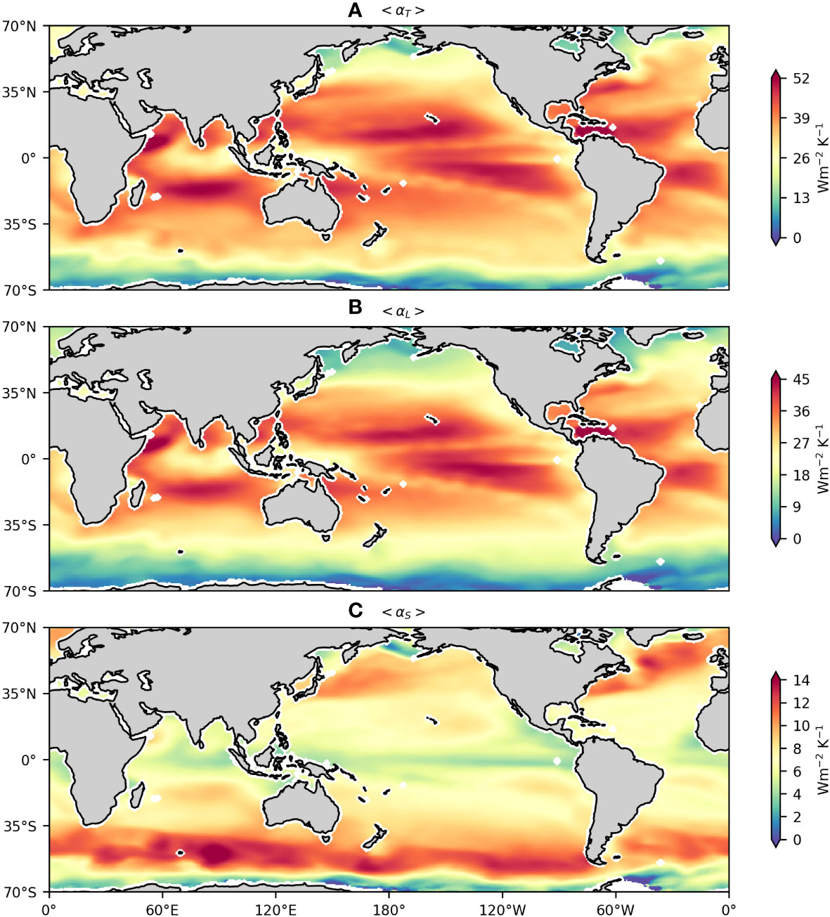
Figure 1 Time-mean (A) α_T , (B) α_L , and (C) α_S in the global ocean during 2008–2020. Note that the colorbars are different for panels (A–C)..

For the computation of Equation. (2), values of $w_{i\text{'},j\text{'}}^{i,j}$ on the land and sea-ice grids are set as zero. To avoid problematic estimation, we confine the regression analysis to 70°S–70°N and discard the estimates of β_i,j within 1.5° from the coastlines.

3 Results

3.1 Spatio-temporal variability of α_T

Figure 1A displays the spatial distribution of the time-mean α_T (denoted as <α_T> henceforth) within 70°S–70°N. There is pronounced spatial variability in <α_T> , with its value ranging from 0 to 52 W/(m² K). The value of <α_T> depends on the latitude, being larger in the tropics than in off-tropical regions and dropping to zero in the Antarctic coastal region. Moreover, <α_T> exhibits evident zonal asymmetry. For instance, in the tropics, <α_T> is more than 40 W/(m² K) in the cold tongues, but the value is reduced to 20 W/(m² K) or so in the Indo-Pacific warm pool. Finally, there is a local enhancement of <α_T> along the major WBCs and their extensions. These spatial features of <α_T> are qualitatively consistent with those of surface total heat flux feedback for mesoscale SSTA reported by Yang et al. (2018), indicating that <α_T> makes a dominant contribution to the surface total heat flux feedback for mesoscale SSTA.

We decompose α_T into the surface latent and sensible heat flux feedbacks, denoted as α_L and α_S , respectively (Figures 1B, C). The magnitude of <α_L> is generally larger than that of <α_S> . The spatial distributions of <α_L> and <α_S> differ substantially from each other. The <α_L> is generally larger in the tropics than in off-tropical regions. The opposite is true for <α_S> . The spatial variability of <α_T> is primarily attributed to <α_L> , with their pattern correlation coefficient reaching up to 0.97. In contrast, the pattern correlation coefficient decreases to 0.11 for <α_S> and <α_T> .

We next examine the temporal variability of α_T measured as the standard deviation of α_T time series (denoted as σ(α_T) henceforth) (Figure 2). The σ(α_T) exhibits banded enhancement in the tropics that is mainly ascribed to σ(α_L) . As to σ(α_T) in the off-tropical regions, there is an evident asymmetry between the two hemispheres: large values of σ(α_T) occurring mainly in the northern hemisphere, particularly under the storm tracks. Both σ(α_L) and σ(α_S) contribute importantly to σ(α_T) there.

FIGURE 2

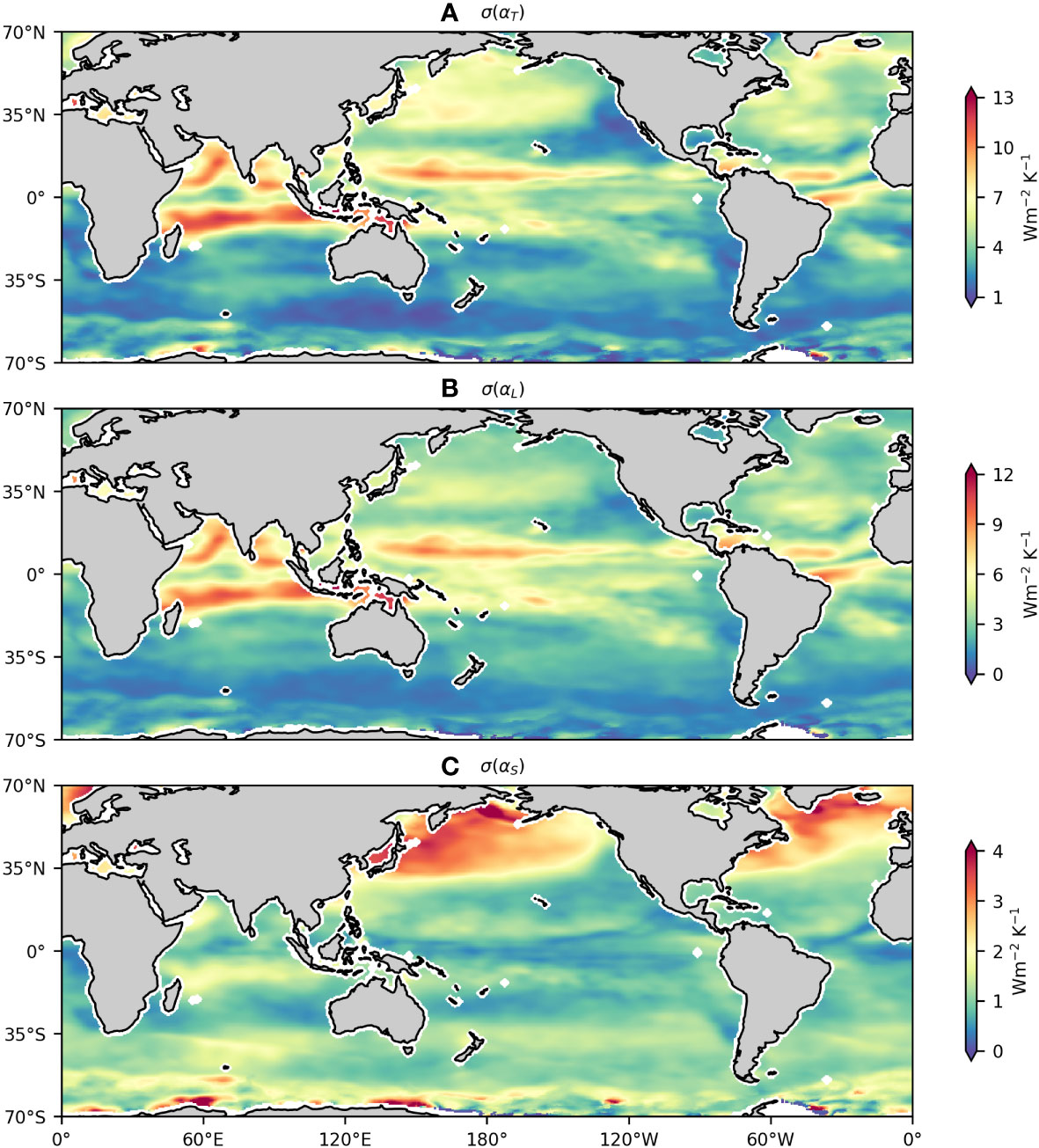
Figure 2 Standard deviation of (A) α_T , (B) α_L , and (C) α_S in the global ocean during 2008–2020. Note that the colorbars are different for panels (A–C).

The temporal variability of α_T is primarily attributed to its prominent seasonal cycle (Figure 3). The global mean σ(α_T) is about 4.0 W/(m² K), about 80% of which is contributed by the seasonal cycle of α_T . Similar is the case for σ(α_S) and σ(α_L) . The peaking season of α_T varies in space. The α_T mostly peaks in autumn or winter off the tropics, whereas it generally peaks in boreal summer or autumn in the tropical region. The peaking seasons of α_L and α_S are the same in many parts of the tropics. However, they differ from each other off the tropics. Specifically, α_L generally reaches its maximum in autumn, whereas α_S peaks in winter.

FIGURE 3

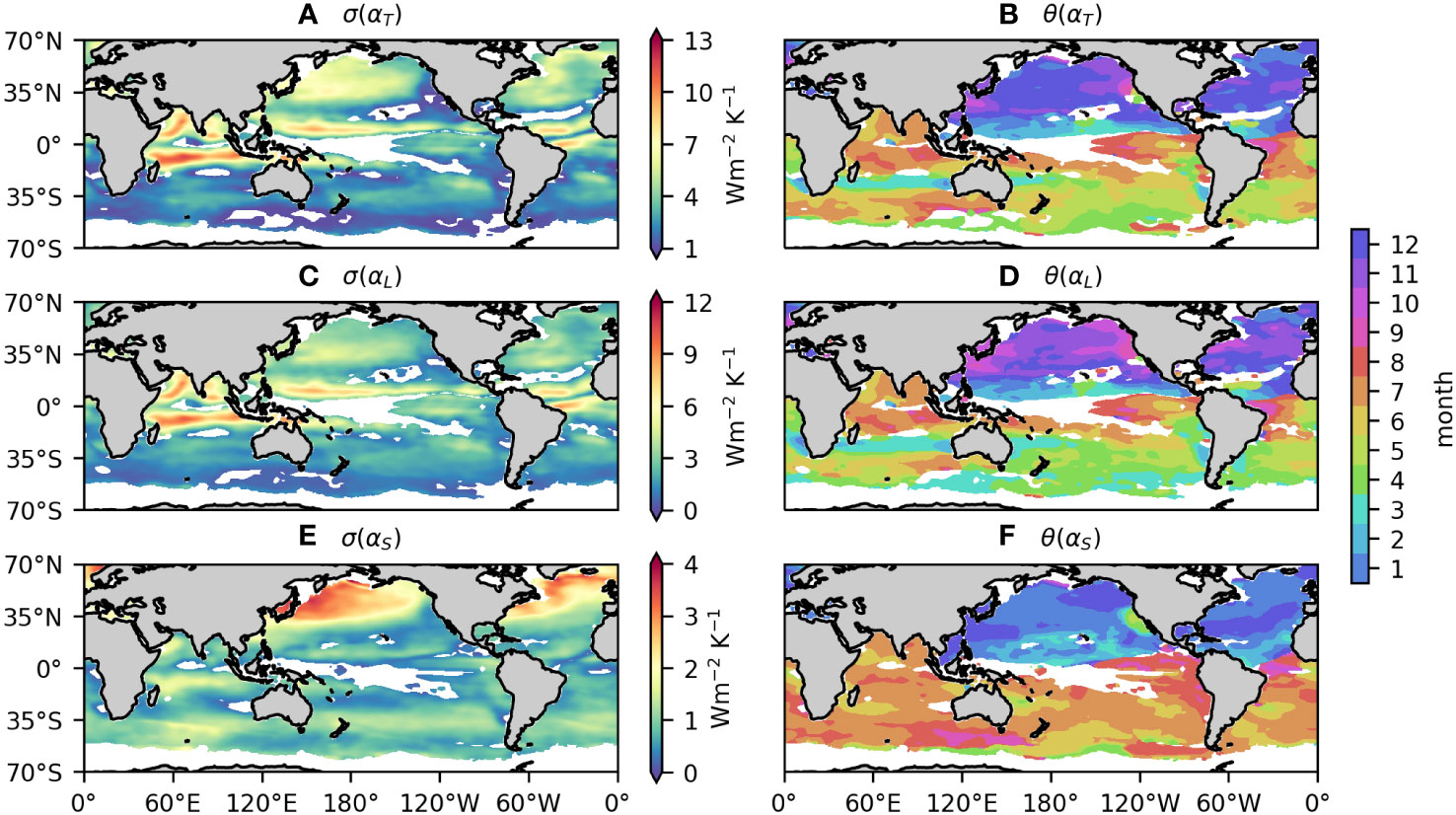
Figure 3 (A) Standard deviation and (B) peaking time of seasonal cycle of α_T in the global ocean during 2008–2020. Here the peaking time of seasonal cycle is defined as the month when α_T reaches its maximum. Regions with statistically insignificant seasonal cycles at the 95% confidence level or seasonally covered by the sea ice are masked by white. (C, D) and (E, F) Same as panels (A, B) but for α_L and α_S , respectively. Note that the colorbars are different for panels (A, C, E).

3.2 Underlying dynamics

In this section, we attempt to uncover the underlying dynamics for the spatio-temporal variability of α_T . The α_L and α_S are controlled by the background atmospheric and oceanic states and different kinds of MABL adjustment to the underlying mesoscale SSTA. Following Hausmann et al. (2017) and Yang et al. (2018), their respective contributions under the assumption of a small magnitude of mesoscale SSTA can be estimated as follows:

$\begin{array}{ll}{\alpha }_{L,A}={\overline{\rho }}_a{\overline{\Lambda }}_V{\overline{C}}_e{\overline{U}}_{10}{\frac{d{q}_{sat}}{dT}|}_{T=\overline{T}}-{\overline{\rho }}_a{\overline{\Lambda }}_V{\overline{C}}_e{\overline{U}}_{10}\frac{d{q}^{\prime }}{d{T}^{\prime }}+{\overline{\rho }}_a{\overline{\Lambda }}_V{\overline{C}}_e\frac{d{U^{\prime }}_{10}}{d{T}^{\prime }}(q_{sat}(\overline{T})-\overline{q})& (4)\end{array}$

$\begin{array}{ll}{\alpha }_{S,A}={\overline{\rho }}_a{\overline{c}}_p{\overline{C}}_h{\overline{U}}_{10}-{\overline{\rho }}_a{\overline{c}}_p{\overline{C}}_h{\overline{U}}_{10}\frac{d{T^{\prime }}_{air}}{d{T}^{\prime }}+{\overline{\rho }}_a{\overline{c}}_p{\overline{C}}_h\frac{d{U^{\prime }}_{10}}{d{T}^{\prime }}(\overline{T}-{\overline{T}}_{air})& (5)\end{array}$

(see Appendix A for derivation details) where ρ_a is the surface (2 m) air density, Λ_V is the latent heat of vaporization, q is the surface (2 m) air-specific humidity, q_sat is its saturated value at SST (denoted as T ), T_air is the surface (2 m) air temperature, U₁₀ is the surface (10 m) wind speed, c_p is the surface (2 m) air-specific heat capacity, and C_e and C_h are the transfer coefficients for evaporation and sensible heat. The overbar and prime denote the large-scale background value and mesoscale anomaly, respectively. The first terms (${\alpha }_{L,A}^B$ and ${\alpha }_{S,A}^B$) on the right-hand side of Equations. (4) and (5) are determined entirely by the background atmospheric and oceanic states. The second terms including the minus signs (${\alpha }_{L,A}^T$ and ${\alpha }_{S,A}^T$) are known as the thermodynamic adjustment and depend on the change of q^′ and T^′_air induced by T^′ . The third terms (${\alpha }_{L,A}^D$ and ${\alpha }_{S,A}^D$), i.e., the dynamic adjustment, originate from the response of U^′₁₀ to T^′. The second and third terms can be estimated by regressing q^′ (T^′_air) and U^′₁₀ onto T^′ based on the GTWR model. It should be noted that the spatio-temporal variability of the second and third terms is not only determined by the MABL adjustment to underlying mesoscale SSTA but also affected by the background atmospheric and oceanic states. The values of α_L,A and α_S,A are found to agree well with α_L and α_S (Figures 4, 5), respectively, lending support to the validity of Equations. (4) and (5).

FIGURE 4

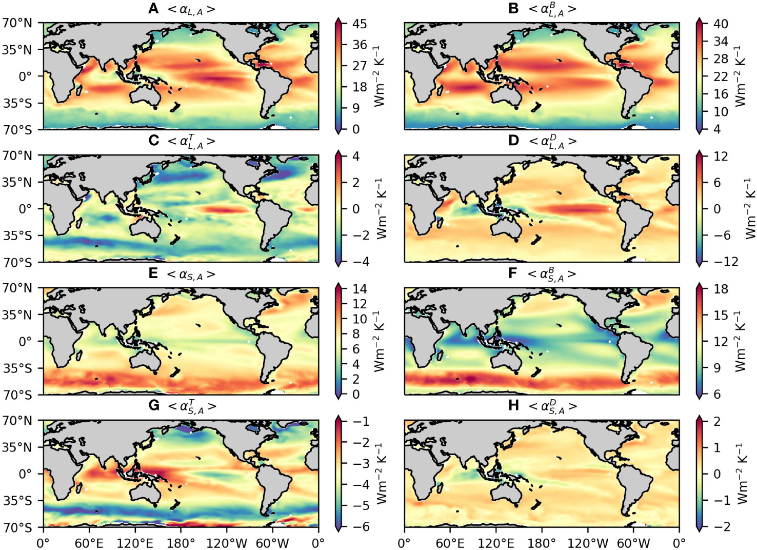
Figure 4 Decomposition of <α_L> into components related to the (B) background atmospheric and oceanic states $<{\alpha }_{L,A}^B>$, (C) thermodynamic adjustment $<{\alpha }_{L,A}^T>$, (D) dynamic adjustment $<{\alpha }_{L,A}^D>$, and (A) the sum of the above three components <α_L,A> . (E–H) Same as panels (A–D) but for <α_S> . Note that the colorbars are different for different panels.

FIGURE 5

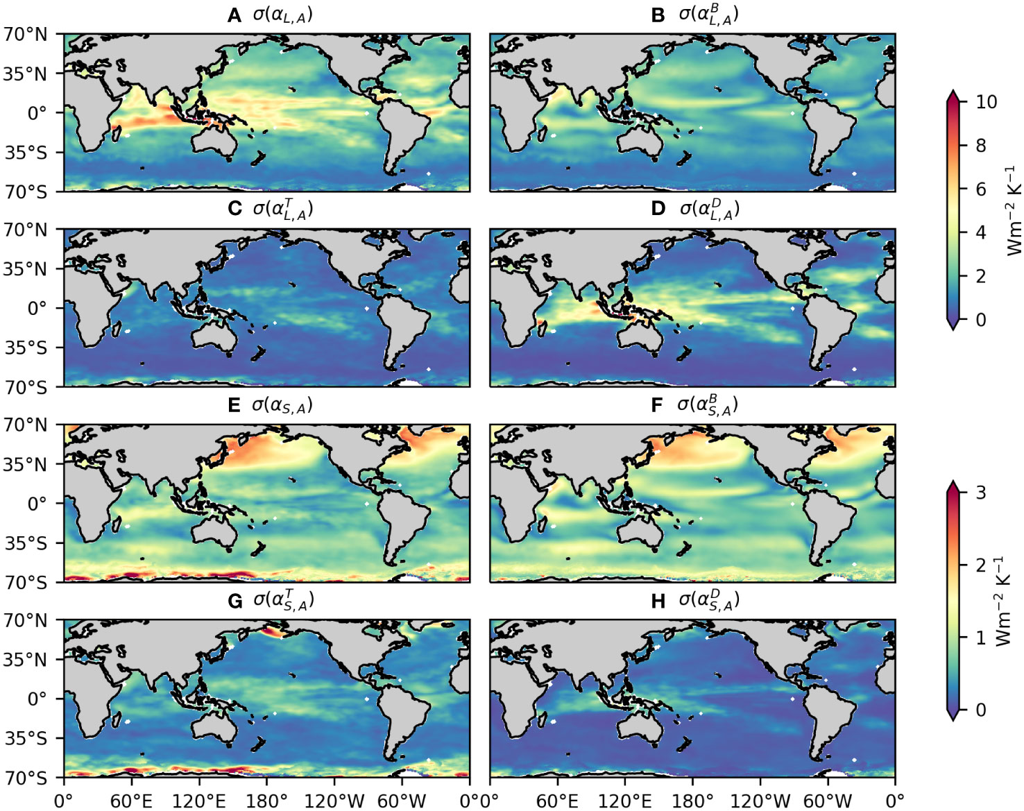
Figure 5 Same as Figure 4 but for σ(α_L) and σ(α_S) .

The spatial variability of <α_L> is largely attributed to $<{\alpha }_{L,A}^B>$ (Figures 4A, B). Their pattern correlation coefficient is 0.97, much larger than 0.31 (0.44) between <α_L> and $<{\alpha }_{L,A}^T>$ ($<{\alpha }_{L,A}^D>$). The spatial pattern of $<{\alpha }_{L,A}^B>$ results primarily from the non-linearity in the Clausius–Clapeyron relation; i.e., ${\frac{d{q}_{sat}}{dT}|}_{T=\overline{T}}$ is an increasing function of $\overline{T}$ (Figure 6A). Such a feature of ${\frac{d{q}_{sat}}{dT}|}_{T=\overline{T}}$ accounts for the larger $<{\alpha }_{L,A}^B>$ in the tropics than off-tropical regions and the minimal $<{\alpha }_{L,A}^B>$ in the Southern Ocean. The spatial inhomogeneity in $<{\overline{U}}_{10}>$ also plays a role (Figures 6C, E). On the one hand, $<{\overline{U}}_{10}>$ is enhanced under the storm tracks, partially compensating for the reduced $<{\alpha }_{L,A}^B>$ off the tropics especially in the Southern Ocean due to ${\frac{d{q}_{sat}}{dT}|}_{T=\overline{T}}$. On the other hand, $<{\overline{U}}_{10}>$ is weakened in the Indo-Pacific warm pool, accounting for the local minimum of $<{\alpha }_{L,A}^B>$ in this region.

FIGURE 6

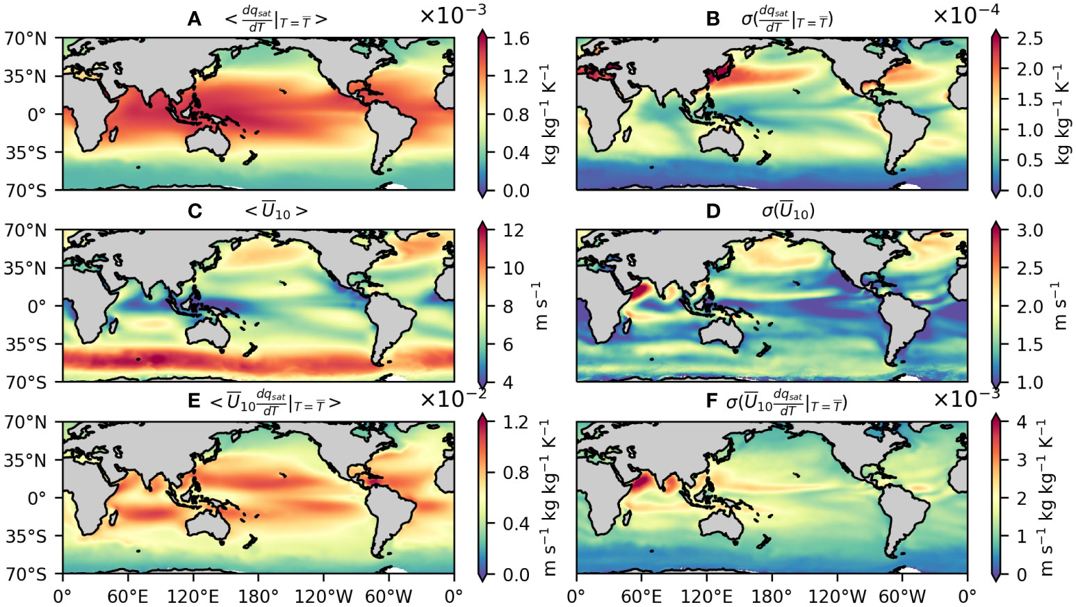
Figure 6 Time-mean (A) ${\frac{d{q}_{sat}}{dT}|}_{T=\overline{T}}$, (C) ${\overline{U}}_{10}$, and (E) their product ${{\overline{U}}_{10}\frac{d{q}_{sat}}{dT}|}_{T=\overline{T}}$ in the global ocean during 2008–2020. (B, D, F) Same as panels (A, C, E) but for the standard deviation of ${\frac{d{q}_{sat}}{dT}|}_{T=\overline{T}}$, ${\overline{U}}_{10}$, and ${{\overline{U}}_{10}\frac{d{q}_{sat}}{dT}|}_{T=\overline{T}}$.

Although $<{\alpha }_{L,A}^B>$ determines the overall spatial structure of <α_L> , there is an evident discrepancy between these two quantities in some parts of the global ocean, suggesting that $<{\alpha }_{L,A}^T>$ and $<{\alpha }_{L,A}^D>$ may be locally important (Figures 4C, D). In particular, <α_L> reaches a local maximum in the equatorial cold tongues, whereas the opposite is true for $<{\alpha }_{L,A}^B>$. This discrepancy is due to the strong adjustment of surface air-specific humidity and wind speed to mesoscale SSTA in these regions. Both $<{\alpha }_{L,A}^T>$ and $<{\alpha }_{L,A}^D>$ contribute positively to <α_L> in the equatorial cold tongues, with their sum comparable to $<{\alpha }_{L,A}^B>$. Moreover, $<{\alpha }_{L,A}^D>$ makes a non-negligible contribution to the enhanced <α_L> along the WBCs and their extensions.

As to <α_S> , its spatial variability is also dominated by that of $<{\alpha }_{S,A}^B>$ with a pattern correlation coefficient of 0.78 (Figures 4E, F). However, $<{\alpha }_{S,A}^B>$ is systematically larger than <α_S> , especially in the off-tropical regions. This bias is mainly attributed to $<{\alpha }_{S,A}^T>$ that is always negative and becomes larger in magnitude as the latitude increases (Figure 4G). The effect of $<{\alpha }_{S,A}^D>$ on <α_S> is generally weaker than that of $<{\alpha }_{S,A}^T>$ but could be locally important in some parts of the global ocean (Figure 4H).

We next examine the underlying dynamics for the temporal variability of α_L and α_S . Both $\sigma ({\alpha }_{L,A}^B)$ and $\sigma ({\alpha }_{L,A}^D)$ make important contributions to σ(α_L) but in different regions (Figures 5A–D). The off-tropical σ(α_L) is mainly attributed to $\sigma ({\alpha }_{L,A}^B)$, whereas $\sigma ({\alpha }_{L,A}^D)$ becomes dominant in the tropics. The temporal variability of ${\alpha }_{L,A}^B$ in the off-tropical region is mainly caused by the combined effects of ${\frac{d{q}_{sat}}{dT}|}_{T=\overline{T}}$ and ${\overline{U}}_{10}$ (Figures 6B, D, F). Recomputing ${\alpha }_{L,A}^B$ by setting ${\frac{d{q}_{sat}}{dT}|}_{T=\overline{T}}$ and ${\overline{U}}_{10}$ as their time-mean values largely suppresses the temporal variability of ${\alpha }_{L,A}^B$ (Figure 7A). As ${\frac{d{q}_{sat}}{dT}|}_{T=\overline{T}}$ and ${\overline{U}}_{10}$ are largest in summer and winter, respectively, their effects on the temporal variability of ${\alpha }_{L,A}^B$ counteract each other. Indeed, taking either ${\frac{d{q}_{sat}}{dT}|}_{T=\overline{T}}$ or ${\overline{U}}_{10}$ alone as its time-mean value will make $\sigma ({\alpha }_{L,A}^B)$ unchanged or even larger (Supplementary Figure S2). This to some extent explains why α_L peaks in autumn off the tropics. As to ${\alpha }_{L,A}^D$, its temporal variability in the tropics is primarily due to dU^′₁₀/dT^′ (Figure 7B), suggesting that the response of surface wind speed to mesoscale SSTA varies evidently with time in this region.

FIGURE 7

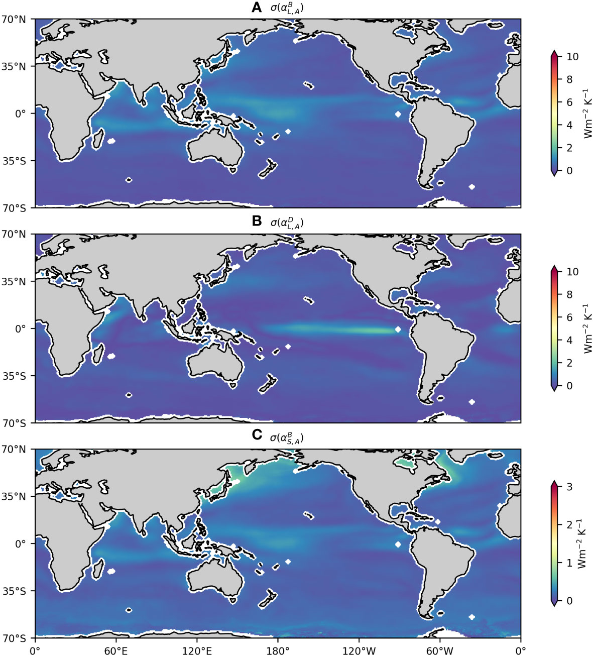
Figure 7 Standard deviation of (A) ${\alpha }_{L,A}^B$recomputed by using time-mean ${\frac{d{q}_{sat}}{dT}|}_{T=\overline{T}}$ and ${\overline{U}}_{10}$, (B) ${\alpha }_{L,A}^D$ recomputed by using time-mean dU^′₁₀/dT^′ , and (C) ${\alpha }_{S,A}^B$ recomputed by using time-mean ${\overline{U}}_{10}$. These quantities should be compared to their counterparts in Figure 5.

The temporal variability of α_S is mainly attributed to $\sigma ({\alpha }_{S,A}^B)$, with $\sigma ({\alpha }_{S,A}^T)$ and $\sigma ({\alpha }_{S,A}^D)$ playing a minor or negligible role (Figures 5E–H). The temporal variability of ${\alpha }_{S,A}^B$ off the tropics results from ${\overline{U}}_{10}$ (Figures 6D, 7C), accounting for the peak of α_S in winter. Finally, it should be noted that the off-tropical temporal variability of ${\frac{d{q}_{sat}}{dT}|}_{T=\overline{T}}$, ${\overline{U}}_{10}$, and their product ${\overline{U}}_{10}{\frac{d{q}_{sat}}{dT}|}_{T=\overline{T}}$ in the northern hemisphere is more evident than their counterpart in the southern hemisphere (Figures 6B, D, F). This contributes to the asymmetry of σ(α_L) and σ(α_S) off the tropics between the two hemispheres.

4 Discussion

The above analysis suggests that the thermodynamic and dynamic adjustments have important effects on the spatio-temporal variability of α_T . In this section, we discuss several notable features of these adjustments that are unexpected from the prevailing thoughts (Barsugli and Battisti, 1998; Xie, 2004; Chelton et al., 2004; Hausmann et al., 2017; Yang et al., 2018). First, classical theories (Barsugli and Battisti, 1998; Hausmann et al., 2017) suggest that the thermodynamic adjustment should reduce α_T because a warm (cold) mesoscale SSTA induces a surface heat and moisture flux anomaly into (out of) the atmosphere, increasing (decreasing) the surface air temperature and specific humidity. However, our results reveal that $<{\alpha }_{L,A}^T>$ is not always negative. In particular, it reinforces <α_L> in the equatorial cold tongues (Figure 4C). This apparently odd feature is not an artifact caused by the GTWR model, as it is also consistently reproduced by the classical constant regression model (Supplementary Figure S3). Instead, it may be explained by the “vertical mixing mechanism” (Wallace et al., 1989; Seo et al., 2007; Chelton and Xie, 2010; Frenger et al., 2013; Putrasahan et al., 2013; Laurindo et al., 2019). A warm mesoscale SSTA heats the MABL from the bottom, reducing the stability and enhancing the vertical mixing in the MABL. The opposite is true for a cold mesoscale SSTA. Due to the large negative vertical gradient of air-specific humidity within the MABL over the equatorial cold tongues (Bond, 1992), the enhanced (weakened) vertical mixing may decrease (increase) the surface air-specific humidity over the warm (cold) mesoscale SSTA, leading to positive $<{\alpha }_{L,A}^T>$. Indeed, the efficacy of the vertical mixing mechanism, measured as the regression coefficient of mesoscale MABL height anomaly onto SSTA, is largest in the equatorial cold tongues (Figure 8).

FIGURE 8

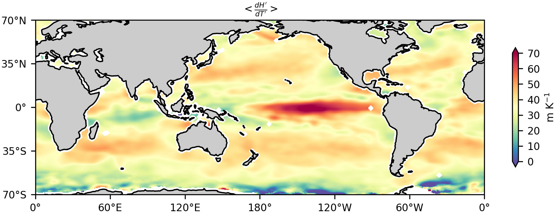
Figure 8 Time-mean regression coefficient of mesoscale MABL height (H) anomaly onto SSTA in the global ocean. MABL, marine atmospheric boundary layer; SSTA, sea surface temperature anomaly.

Second, it is generally thought that the mesoscale air–sea interactions could cause a positive correlation between U^′₁₀ and T^′ via the vertical momentum mixing or pressure gradient effects (Lindzen and Nigam, 1987; Chelton et al., 2004; Xie, 2004; Small et al., 2008; Chelton and Xie, 2010; Frenger et al., 2013; Ma et al., 2015; Laurindo et al., 2019) so that the dynamic adjustment increases α_T . Such a thought is consistent with the positive $<{\alpha }_{L,A}^D>$ and $<{\alpha }_{S,A}^D>$ over the majority of the global ocean. However, there are some regions where $<{\alpha }_{L,A}^D>$ and $<{\alpha }_{S,A}^D>$ are significantly negative, especially in the Indo-Pacific warm pool. These negative values are not an artifact of the GTWR model (Supplementary Figure S4). As the regression analysis cannot distinguish the cause and effect, one possibility might be that the negative $<{\alpha }_{L,A}^D>$ and $<{\alpha }_{S,A}^D>$ there reflect the forced response of T^′ by U^′₁₀ . A positive U^′₁₀ could generate a negative T^′ by increasing the heat flux out of the ocean and entrainment of cooler thermocline water into the surface layer. At this stage, the underlying dynamics for the negative correlation between U^′₁₀ and T^′ remains unknown and deserves further analysis in future studies.

5 Conclusions

In this study, we quantify the spatio-temporal variability of surface turbulent heat flux feedback for mesoscale SSTA over the global ocean, based on the GTWR model. The major conclusions are summarized as follows.

First, there is pronounced spatial variability in <α_T> with its value generally ranging from 0 to 50 W/(m² K) within 70°S–70°N. It is larger in the tropics than off-tropical regions and shows local enhancement in the equatorial cold tongues and WBCs as well as their extensions. The overall spatial pattern of <α_T> is primarily attributed to the non-linear Clausius–Clapeyron relation and inhomogeneous background wind speed. The thermodynamic and dynamic adjustments play an important role in the regional variability, accounting for the large <α_T> in the equatorial cold tongues and contributing to the enhanced <α_T> along the WBCs as well as their extensions.

Second, the temporal variability of α_T is mainly ascribed to its seasonal cycle. The amplitude and peaking time of α_T seasonal cycle vary in space. The strong seasonal cycle occurs in the tropics and under the storm tracks in the northern hemisphere. The former is primarily caused by the seasonally varying response of surface wind speed to mesoscale SSTA, whereas the latter is due to the seasonality of background atmospheric and oceanic states.

The superiority of the GTWR model over the classical constant regression model enables it to uncover more features of α_T that have not been reported by previous studies. Nevertheless, the GTWR model is incapable of analyzing any potential non-linearity in α_T , e.g., the dependence of α_T on the magnitude of mesoscale SSTA (e.g., Moreton et al., 2021) and the asymmetry of α_T between warm and cold mesoscale SSTA. These issues deserve analysis in future studies but require more advanced regression models.

Data availability statement

The original contributions presented in the study are included in the article/Supplementary Material. Further inquiries can be directed to the corresponding author.

Author contributions

All authors contributed to the manuscript and approved the submitted version.

Funding

This research is supported by the National Science Foundation of China (41906011).

Acknowledgments

We thank Dr. Fengfei Song for his insightful advice. The transfer coefficients for evaporation and sensible heat in the bulk formula are calculated by AeroBulk (https://github.com/brodeau/aerobulk) (Brodeau et al., 2017).

Conflict of interest

The authors declare that the research was conducted in the absence of any commercial or financial relationships that could be construed as a potential conflict of interest.

Publisher’s note

All claims expressed in this article are solely those of the authors and do not necessarily represent those of their affiliated organizations, or those of the publisher, the editors and the reviewers. Any product that may be evaluated in this article, or claim that may be made by its manufacturer, is not guaranteed or endorsed by the publisher.

Supplementary material

The Supplementary Material for this article can be found online at: https://www.frontiersin.org/articles/10.3389/fmars.2022.957796/full#supplementary-material

References

Barsugli J. J., Battisti ,. D. S. (1998). The basic effects of atmosphere–ocean thermal coupling on midlatitude variability*. J. Atmos. Sci. 55, 477–493. doi: 10.1175/1520-0469(1998)055<0477:TBEOAO>2.0.CO;2

CrossRef Full Text | Google Scholar

Bishop S. P., Small R. J., Bryan F. O. (2020). The global sink of available potential energy by mesoscale air-Sea interaction. J. Adv. Model. Earth Syst. 12, e2020MS002118. doi: 10.1029/2020MS002118

PubMed Abstract | CrossRef Full Text | Google Scholar

Bond N. A. (1992). Observations of planetary boundary-layer structure in the Eastern equatorial pacific. J. Clim. 5, 699–706. doi: 10.1175/1520-0442(1992)005<0699:OOPBLS>2.0.CO;2

CrossRef Full Text | Google Scholar

Brodeau L., Barnier B., Gulev S. K., Woods C. (2017). Climatologically significant effects of some approximations in the bulk parameterizations of turbulent air–Sea fluxes. J. Phys. Oceanogr. 47, 5–28. doi: 10.1175/JPO-D-16-0169.1

CrossRef Full Text | Google Scholar

Brunsdon C., Fotheringham A. S., Charlton M. E. (1996). Geographically weighted regression: A method for exploring spatial nonstationarity. Geogr. Anal. 28, 281–298. doi: 10.1111/J.1538-4632.1996.TB00936.X

CrossRef Full Text | Google Scholar

Bryan F. O., Tomas R., Dennis J. M., Chelton D. B., Loeb N. G., Mcclean J. L. (2010). Frontal scale air-sea interaction in high-resolution coupled climate models. J. Clim. 23, 6277–6291. doi: 10.1175/2010JCLI3665.1

CrossRef Full Text | Google Scholar

Chelton D. B., Schlax M. G., Freilich M. H., Milliff R. F. (2004). Satellite measurements reveal persistent small-scale features in ocean winds. Sci. (80-. ) 303(5660), 978–983. doi: 10.1126/science.1091901

CrossRef Full Text | Google Scholar

Chelton D., Xie S.-P. (2010). Coupled ocean-atmosphere interaction at oceanic mesoscales. Oceanography 23, 52–69. doi: 10.5670/oceanog.2010.05

CrossRef Full Text | Google Scholar

Fotheringham A. S., Brunsdon C., Charlton M. (2002). Geographically weighted regression: The analysis of spatially varying relationships. 269. The Atrium, Southern Gate, Chichester, West Sussex PO19 8SQ, England: John Wiley & Sons Ltd.

Google Scholar

Fotheringham A., Charlton M., Brunsdon C. (1996). The geography of parameter space: An investigation of spatial non-stationarity. Int. J. Geogr. Inf. Syst. 10, 605–627. doi: 10.1080/02693799608902100

CrossRef Full Text | Google Scholar

Fotheringham A. S., Crespo R., Yao J. (2015). Geographical and temporal weighted regression (GTWR). Geogr. Anal. 47, 431–452. doi: 10.1111/gean.12071

CrossRef Full Text | Google Scholar

Frankignoul C. (1985). Sea Surface temperature anomalies, planetary waves, and air-sea feedback in the middle latitudes. Rev. Geophys. 23, 357. doi: 10.1029/RG023i004p00357

CrossRef Full Text | Google Scholar

Frankignoul C., Czaja A., L’Heveder B. (1998). Air–Sea feedback in the north Atlantic and surface boundary conditions for ocean models. J. Clim. 11, 2310–2324. doi: 10.1175/1520-0442(1998)011<2310:ASFITN>2.0.CO;2

CrossRef Full Text | Google Scholar

Frankignoul C., Hasselmann K. (1977). Stochastic climate models, part II application to sea-surface temperature anomalies and thermocline variability. Tellus 29, 289–305. doi: 10.3402/tellusa.v29i4.11362

CrossRef Full Text | Google Scholar

Frankignoul C., Kestenare E. (2002). The surface heat flux feedback. part I: Estimates from observations in the Atlantic and the north pacific. Clim. Dyn. 19, 633–648. doi: 10.1007/s00382-002-0252-x

CrossRef Full Text | Google Scholar

Frenger I., Gruber N., Knutti R., Münnich M. (2013). Imprint of southern ocean eddies on winds, clouds and rainfall. Nat. Geosci. 6, 608–612. doi: 10.1038/ngeo1863

CrossRef Full Text | Google Scholar

Guo Y., Bishop S., Bryan F., Bachman S. (2022). A global diagnosis of eddy potential energy budget in an eddy permitting ocean model. J. Phys. Oceanogr. 52(8), 1731–1748. doi: 10.1175/JPO-D-22-0029.1

CrossRef Full Text | Google Scholar

Hausmann U., Czaja A. (2012). The observed signature of mesoscale eddies in sea surface temperature and the associated heat transport. Deep. Res. Part I Oceanogr. Res. Pap. 70, 60–72. doi: 10.1016/j.dsr.2012.08.005

CrossRef Full Text | Google Scholar

Hausmann U., Czaja A., Marshall J. (2016). Estimates of air-sea feedbacks on sea surface temperature anomalies in the southern ocean. J. Clim. 29, 439–454. doi: 10.1175/JCLI-D-15-0015.1

CrossRef Full Text | Google Scholar

Hausmann U., Czaja A., Marshall J. (2017). Mechanisms controlling the SST air-sea heat flux feedback and its dependence on spatial scale. Clim. Dyn. 48, 1297–1307. doi: 10.1007/s00382-016-3142-3

CrossRef Full Text | Google Scholar

Hersbach H., Bell B., Berrisford P., Hirahara S., Horányi A., Muñoz-Sabater J., et al. (2020). The ERA5 global reanalysis. Q. J. R. Meteorol. Soc 146, 1999–2049. doi: 10.1002/qj.3803

CrossRef Full Text | Google Scholar

Huang B., Wu B., Barry M. (2010). Geographically and temporally weighted regression for modeling spatio-temporal variation in house prices. Int. J. Geogr. Inf. Sci. 24, 383–401. doi: 10.1080/13658810802672469

CrossRef Full Text | Google Scholar

Large W. G., Yeager S. G. (2004). Diurnal to decadal global forcing for ocean and sea-ice models: The data sets and flux climatologies. doi: 10.5065/D6KK98Q6

CrossRef Full Text | Google Scholar

Laurindo L. C., Siqueira L., Mariano A. J., Kirtman B. P. (2019). Cross-spectral analysis of the SST/10-m wind speed coupling resolved by satellite products and climate model simulations. Clim. Dyn. 52, 5071–5098. doi: 10.1007/s00382-018-4434-6

CrossRef Full Text | Google Scholar

Lindzen R. S., Nigam S. (1987). On the role of Sea surface temperature gradients in forcing low-level winds and convergence in the tropics. J. Atmos. Sci. 44, 2418–2436. doi: 10.1175/1520-0469(1987)044<2418:OTROSS>2.0.CO;2

CrossRef Full Text | Google Scholar

Li F., Sang H., Jing Z. (2017). Quantify the continuous dependence of SST-turbulent heat flux relationship on spatial scales. Geophys. Res. Lett. 44, 6326–6333. doi: 10.1002/2017GL073695

CrossRef Full Text | Google Scholar

Ma X., Jing Z., Chang P., Liu X., Montuoro R., Small R. J., et al. (2016). Western Boundary currents regulated by interaction between ocean eddies and the atmosphere. Nature 535, 533–537. doi: 10.1038/nature18640

PubMed Abstract | CrossRef Full Text | Google Scholar

Ma J., Xu H., Dong C., Lin P., Liu Y. (2015). Atmospheric responses to oceanic eddies in the kuroshio extension region. J. Geophys. Res. Atmos. 120, 6313–6330. doi: 10.1002/2014JD022930

CrossRef Full Text | Google Scholar

Moreton S., Ferreira D., Roberts M., Hewitt H. (2021). Air-Sea turbulent heat flux feedback over mesoscale eddies. Geophys. Res. Lett. 48, e2021GL095407. doi: 10.1029/2021GL095407

CrossRef Full Text | Google Scholar

Park S., Deser C., Alexander M. A. (2005). Estimation of the surface heat flux response to Sea surface temperature anomalies over the global oceans. J. Clim. 18, 4582–4599. doi: 10.1175/JCLI3521.1

CrossRef Full Text | Google Scholar

Putrasahan D. A., Miller A. J., Seo H. (2013). Isolating mesoscale coupled ocean–atmosphere interactions in the kuroshio extension region. Dyn. Atmos. Ocean. 63, 60–78. doi: 10.1016/j.dynatmoce.2013.04.001

CrossRef Full Text | Google Scholar

Seo H., Miller A. J., Roads J. O. (2007). The Scripps coupled ocean–atmosphere regional (SCOAR) model, with applications in the Eastern pacific sector. J. Clim. 20, 381–402. doi: 10.1175/JCLI4016.1

CrossRef Full Text | Google Scholar

Shan X., Jing Z., Gan B., Wu L., Chang P., Ma X., et al. (2020a). Surface heat flux induced by mesoscale eddies cools the kuroshio-oyashio extension region. Geophys. Res. Lett. 47, e2019GL086050. doi: 10.1029/2019GL086050

CrossRef Full Text | Google Scholar

Shan X., Jing Z., Sun B., Chang P., Wu L., Ma X. (2020b). Influence of the ocean mesoscale eddy–atmosphere thermal feedback on the upper-ocean haline stratification. J. Phys. Oceanogr. 50, 2475–2490. doi: 10.1175/JPO-D-19-0193.1

CrossRef Full Text | Google Scholar

Small R. J., Bryan F. O., Bishop S. P., Tomas R. A. (2019). ). air–Sea turbulent heat fluxes in climate models and observational analyses: What drives their variability? J. Clim. 32, 2397–2421. doi: 10.1175/JCLI-D-18-0576.1

CrossRef Full Text | Google Scholar

Small R. J., deSzoeke S. P., Xie S. P., O’Neill L., Seo H., Song Q., et al. (2008). Air–sea interaction over ocean fronts and eddies. Dyn. Atmos. Ocean. 45, 274–319. doi: 10.1016/j.dynatmoce.2008.01.001

CrossRef Full Text | Google Scholar

Wallace J. M., Mitchell T. P., Deser C. (1989). The influence of Sea-surface temperature on surface wind in the Eastern equatorial pacific: Seasonal and interannual variability. J. Clim. 2, 1492–1499. doi: 10.1175/1520-0442(1989)002<1492:TIOSST>2.0.CO;2

CrossRef Full Text | Google Scholar

Xie S.-P. (2004). Satellite observations of cool ocean–atmosphere interaction. Bull. Am. Meteorol. Soc 85, 195–208. doi: 10.1175/BAMS-85-2-195

CrossRef Full Text | Google Scholar

Yang H., Chang P., Qiu B., Zhang Q., Wu L., Chen Z., et al. (2019). Mesoscale air–Sea interaction and its role in eddy energy dissipation in the kuroshio extension. J. Clim. 32, 8659–8676. doi: 10.1175/JCLI-D-19-0155.1

CrossRef Full Text | Google Scholar

Yang P., Jing Z., Wu L. (2018). An assessment of representation of oceanic mesoscale eddy-atmosphere interaction in the current generation of general circulation models and reanalyses. Geophys. Res. Lett. 45, 11,856–11,865. doi: 10.1029/2018GL080678

CrossRef Full Text | Google Scholar

Appendix A derivations of equations (4) and (5)

According to the bulk formula (Large and Yeager, 2004), latent (Q_L ) and sensible heat fluxes (Q_S ) can be formulated as follows:

$\begin{array}{ll}{Q}_L={\rho }_a{\Lambda }_V{C}_e{U}_{10}(q_{sat}-q)& \text{(A1)}\end{array}$

$\begin{array}{ll}{Q}_S={\rho }_a{c}_p{C}_h{U}_{10}(T-T_{air})& \text{(A2)}\end{array}$

where Q_L and Q_S are defined positive upwards.

Decompose the quantities in Equations. (A1) and (A2) into the large-scale background values and mesoscale anomalies. Linearizing Equations. (A1) and (A2) with respect to the mesoscale anomalies yields the following:

$\begin{array}{ll}{Q^{\prime }}_L={\overline{\rho }}_a{\overline{\Lambda }}_V{\overline{C}}_e{\overline{U}}_{10}\left({\frac{d{q}_{sat}}{dT}|}_{T=\overline{T}}·T^{\prime }-q^{\prime }\right)+{\overline{\rho }}_a{\overline{\Lambda }}_V{\overline{C}}_e{U^{\prime }}_{10}(q_{sat}(\overline{T})-\overline{q})& \text{(A3)}\end{array}$

$\begin{array}{ll}{Q^{\prime }}_S={\overline{\rho }}_a{\overline{c}}_p{\overline{C}}_h{\overline{U}}_{10}(T^{\prime }-{T^{\prime }}_{air})+{\overline{\rho }}_a{\overline{c}}_p{\overline{C}}_h{U^{\prime }}_{10}(\overline{T}-{\overline{T}}_{air})& \text{(A4)}\end{array}$

where we have dropped the mesoscale anomalies for ρ_a , Λ_V , c_p , C_e , and C_h , as these terms are negligible. Differentiating Equations. (A3) and (A4) with respect to T^′ yields Equations. (4) and (5).