 Chong Sun
 Chengyan Liu
 Zhaomin Wang
 Liangjun Yan1
- 1Key Laboratory of Marine Hazards Forecasting, Ministry of Natural Resources, Hohai University, Nanjing, China/College of Oceanography, Hohai University, Nanjing, China
- 2Southern Marine Science and Engineering Guangdong Laboratory, Zhuhai, China
The bathymetry around Antarctica can govern the shelf sea circulations and play a key role in conditioning water masses. In Prydz Bay, the Prydz Bay Gyre and coastal currents are also determined by the continental shelf topography. However, due to the paucity of beam echo sounding data, the bathymetric datasets in Prydz Bay still have large uncertainties. With the aid of in situ hydrographic observations, this study focuses on the correction of an up-to-date bathymetric dataset and the resultant influences on the shelf circulation and the basal melting of the ice shelves. The corrected bathymetry mainly improves the biased shallow representations in the uncorrected bathymetric data set, with a maximum change of ~500 m deepening in the eastern flank of Prydz Bay. Sensitivity numerical experiments show that the bathymetric corrections in Prydz Bay have a significant impact on the circulation pattern and onshore warm water intrusions. In addition, the corrected bathymetry markedly decreases the heat transport towards the calving front of the Amery Ice Shelf. The onshore heat transport reduces by ~22.18% from ~5.23×10¹³ J s-1 to ~4.07×10¹³ J s-1 over the outer shelf. Over the inner shelf, the heat transport towards the Amery Ice Shelf reduces by ~18.15% from ~5.95×10¹³ J s-1 to ~4.87×10¹³ J s-1. Consequently, the temporally and spatially averaged basal melting rate of the Amery Ice Shelf reduces by ~13.04% from ~0.69 m yr-1 to ~0.60 m yr-1.
1 Introduction
Satellite-based observations have revealed that the mass loss of the Antarctic ice sheet is primarily induced by the ocean-driven basal melting of Antarctic ice shelves (Rignot et al., 2013; Liu et al., 2015; Adusumilli et al., 2020). Ice shelves, as the extensions of grounding ice sheets into the ocean, act to buttress the ice sheet Dupont and Alley, 2005) , and thereby the retreat of the ice shelves can accelerate the ice streams into the ocean. Many ice shelves have been experiencing a net mass loss and thinning due to the enhanced ocean-driven basal melting (Adusumilli et al., 2020). The basal melting of ice shelves is directly affected by the circulations over the Antarctic continental shelf (Rignot et al., 2013), with cross-shelf heat transport delivered into the sub-ice-shelf cavities (Herraiz-Borreguero et al., 2015; Nitsche et al., 2017; Nakayama et al., 2019; Tinto et al., 2019). In addition, the ice shelf basal melting has also been confirmed to be a major driver of ice shelf calving (Liu et al., 2015). However, the in situ measurements are so limited that it is difficult to directly assess the oceanic contribution to the ice shelf basal melting based on hydrographic observations. Numerical models can shed light on our understanding of the interactions between ice shelves and the ocean. To simulate the response of ice shelves to the changes of oceanic circulation and water masses, it is important to properly represent the circulations and water mass properties over the Antarctica continental shelf in numerical models (Rignot and Jacobs, 2002; Reese et al., 2018) .
There are, however, some uncertainties in the existing numerical simulations of the Antarctic shelf sea. Specifically, several factors can cause large uncertainties in the numerical simulations, such as the inaccuracy in the bottom topography and the geometry of the sub-ice-shelf cavities (Liu et al., 2017; Liu et al., 2018; Millan et al., 2020), the coarse model resolution (Stewart et al., 2018), the biases in the atmospheric forcing field (Large and Danabasoglu, 2006; Brodeau et al., 2010; Barthélemy et al., 2018) . In this study, we intend to illustrate how the corrections in the continental shelf topography affect the simulated shelf sea circulation, water mass properties, and the ice shelf basal melting in Prydz Bay.
It has long been realized that the bottom topography is of great importance to the oceanic circulation pattern and the ecosystem in the shelf sea regions (Graham et al., 2011; Dickens et al., 2014; Liu et al., 2018; Millan et al., 2020). Previous studies have shown that the bathymetry of the Antarctica continental slope directly controls the water mass exchanges between the deep ocean and the shelf seas (Walker et al., 2007; Thoma et al., 2008; Nicholls et al., 2009; Hellmer et al., 2012; Pritchard et al., 2012), especially for the intrusion of modified Circumpolar Deep Water (mCDW) onto the continental shelf (Nitsche et al., 2007; Millan et al., 2017; Nitsche et al., 2017; Tinto et al., 2019). Therefore, the accurate high-resolution ocean bathymetry data is favorable in precisely delineating the pathways of mCDW onshore intrusion and consequent influences on the ice shelf melting rates (Nakayama et al., 2019; Goldberg et al., 2020; Eisermann et al., 2021). The bottom topography can also regulate the tidal dynamics and hence their impacts on the ice shelf melting and stability (Padman et al., 2002; Griffiths and Peltier, 2009; Makinson et al., 2011; Rosier et al., 2014; Padman et al., 2018). Furthermore, the accuracy of the bathymetric data is essential for our understanding of the ecology of Antarctic marine flora and fauna (Ribic et al., 2008; Smith et al., 2021). For example, the krill concentration that regulates the distribution and breeding success of Antarctic mammals is severely affected by the bathymetry (McConnell et al., 1992; Ribic et al., 2008; Smith et al., 2021).
Despite the importance of bathymetry, logistical difficulties still leave most of the Antarctic shelf seas uncharted (Arndt et al., 2013; Mayer et al., 2018). In situ bathymetry measurements in most Antarctic shelf regions are still sparse due to the harsh environment and the intensive sea ice coverage (Padman et al., 2010; Arndt et al., 2013). Therefore, the directly measured data sources are so sparse around the Antarctic margins that the insufficiently surveyed bathymetry may overlook some significant topographical features (Arndt et al., 2013). Over the areas without any cruise approaches, the estimation of bathymetry mainly relies on the satellite-based gravity measurements, resulting in large uncertainties and a relatively coarse resolution (Sandwell and Smith, 2001) .
Since the uncertainties of the bathymetry seriously limit our understanding of seafloor morphology around the Antarctica margins, previous studies have taken a variety of approaches to improve the accuracy of the bathymetric data sets (Nitsche et al., 2007; Beaman et al., 2011; Graham et al., 2011; Dickens et al., 2014; Millan et al., 2017; Millan et al., 2020; Smith et al., 2021). To construct an improved bathymetry data set for the Antarctic shelf seas, it is a conventional and effective way of conducting the single beam and multibeam measurements with shipborne echo soundings during a number of expeditions (Nitsche et al., 2007; Beaman et al., 2011; Graham et al., 2011; Dickens et al., 2014; Smith et al., 2021). Airborne gravity provides an efficient remote sensing approach to reconstruct the detailed geometry of sub-ice-shelf cavities (Millan et al., 2017; Cochran et al., 2020; Millan et al., 2020; Eisermann et al., 2021; Yang et al., 2021). Importantly, marine mammals equipped with conductivity-temperature-depth satellite relay data loggers (CTD‐SRDLs), which have greatly enriched the traditional hydrographic data sets (Hooker and Boyd, 2003; Padman et al., 2010; Herraiz‐Borreguero et al., 2016; Williams et al., 2016) , also offer the further possibility to explore the bathymetry of the Antarctic continental shelf. Based on the seafloor depth inferred from the maximum dive depth of the equipped elephant seal, Padman et al. (2010) have improved the bathymetry of the troughs across the continental shelf in the southern Bellingshausen Sea.
In recent years, some studies have investigated the influences of the high-resolution bathymetry on the ocean circulations over the continental shelf and in the sub-ice-shelf cavities (Millan et al., 2017; Nitsche et al., 2017; Cochran et al., 2020). Previous studies have shown that the detailed representation of the bathymetry is critical to properly simulate the cross-shelf transport of warm water into the sub-ice-shelf cavities (Millan et al., 2017; Nitsche et al., 2017; Millan et al., 2020). Numerical studies have also focused on the influences of the high-resolution sub-ice-shelf geometry on the circulations under the ice shelf and the ice shelf basal melting (Goldberg et al., 2020; Millan et al., 2020). Despite that some corrected high-resolution bathymetry data sets of the Antarctic continental shelf have been compiled (Dickens et al., 2014; Nitsche et al., 2017; Smith et al., 2021; Tao et al., 2021), the influences of the bathymetry corrections on the circulations, water mass properties, and the basal melting of ice shelves have not been clarified.
In this study, with the aid of a coupled regional ocean-sea ice-ice shelf model for Prydz Bay, we intend to investigate the ocean circulation, water masses, and the AIS basal melting in response to the correction of a high-resolution bathymetric data set. In section 2, we review several earlier bathymetry datasets and one recent bathymetry dataset in Prydz Bay and introduce the numerical model employed in this study. We then compare the model results from two sensitivity experiments to reveal the impacts of the bathymetry correction on the simulated circulations, water properties, and the AIS basal melting rate in section 3. A summary is given in section 4.
2 Data and model
2.1 Bathymetric data in Prydz Bay
Several global or hemispheric-scale bathymetric datasets have been released, such as RTopo-1 (Timmermann et al., 2010), IBCSO V1 (Arndt et al., 2013), RTopo-2 (Schaffer et al., 2016), GEBCO_2014 (Weatherall et al., 2015), GEBCO_2019 (GEBCO Bathymetric Compilation Group, 2019). Several recent bathymetric datasets basically refer to IBCSO V1 for the bathymetry of the Southern Ocean. So IBCSO V1 also remains as one of the most advanced Digital Bathymetry Model (DBM) for the Southern Ocean region (Becker et al., 2009; Arndt et al., 2013; Weatherall et al., 2015; Mayer et al., 2018). IBCSO is a regional mapping project of the General Bathymetric Chart of the Oceans (GEBCO), which aims to produce high-resolution bathymetric maps of the sea around the Antarctic continent (Arndt et al., 2013). The IBCSO Version 1.0 DBM, released in 2013, is based on all available bathymetric data collected by more than 30 institutions from 15 countries and covers the area south of 60°S with a resolution of 500 × 500 m (Arndt et al., 2013). In fact, in the IBCSO V1, only ~ 17% of the grid cells in the whole Southern Ocean region are directly constrained by the observations, while the rest are determined by interpolation between the measured values or by integrating the predicted water depth (Arndt et al., 2013). In Prydz Bay, the fraction of grid cells constrained by the beam echo soundings is lower than ~5%. Overall, the bathymetry in Prydz Bay is still poorly constrained over a broad region (Figure 1A), and some significant topographical features may not have been identified.
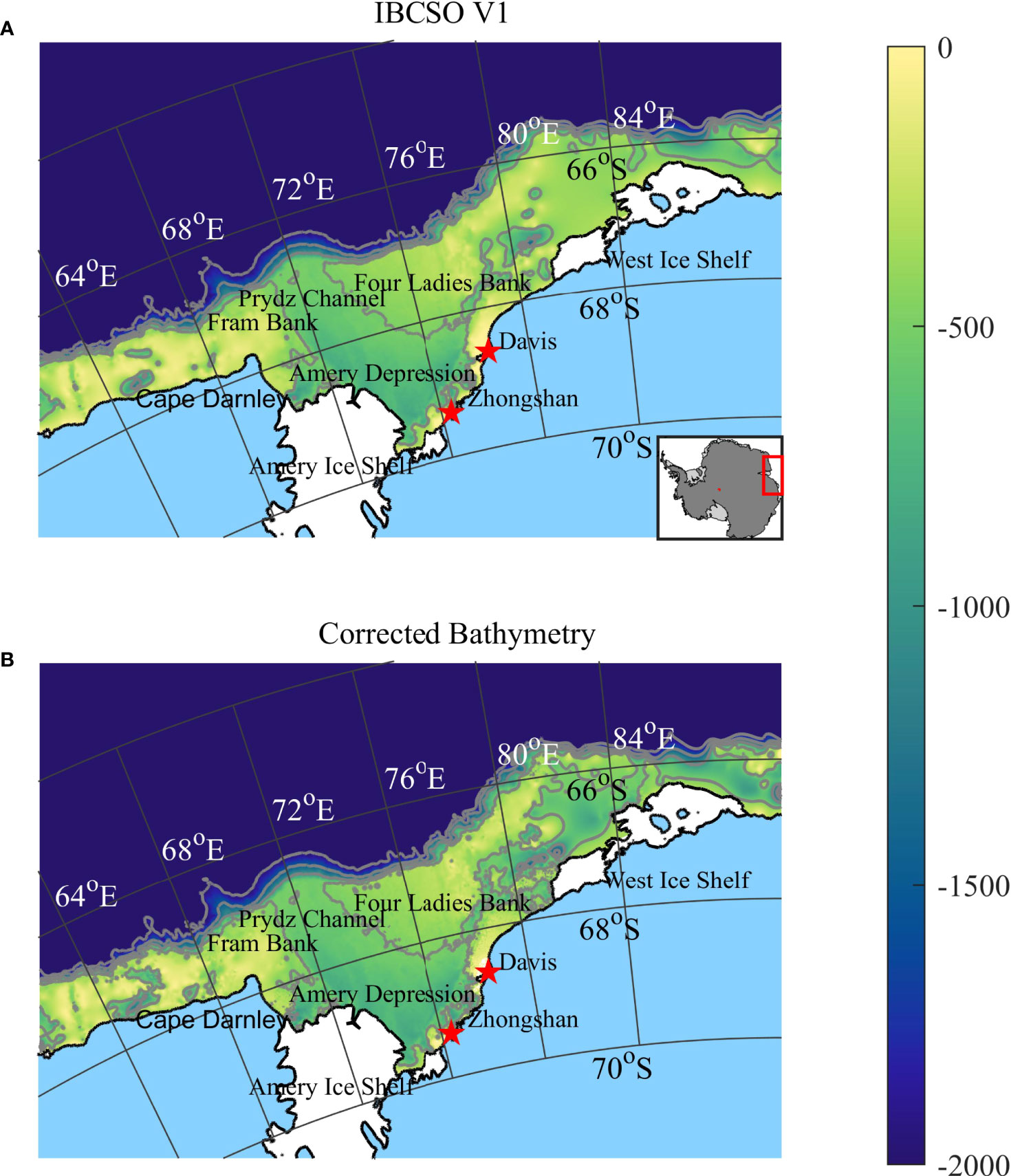
Figure 1 (A) Bathymetry (m) for Prydz Bay from IBCSO Version 1.0. Ice shelves, main topographical features, and the research stations (red stars) are marked at the corresponding locations. Ice shelves are shaded in white, and the land is shaded in light blue. The grey lines are bathymetric contours from IBCSO V1 from 500 to 2000 m with an interval of 500 m. (B) Same as (A), but for the CB (m).
RTopo-2 is a common bathymetric data used for the high-resolution simulations focused on the Antarctic shelf seas (Liu et al., 2018; Zaron, 2019; Daae et al., 2020). As a global bathymetric dataset, RTopo-2 is a combination of two bathymetric datasets (Schaffer et al., 2016): 1) IBCSO V1 for the Southern Ocean and the shelf seas around Antarctica (Arndt et al., 2013; Schaffer et al., 2016), and 2) Bedmap2 for the Antarctic ice sheet/shelf surface height, thickness and bedrock bathymetry (Fretwell et al., 2013; Schaffer et al., 2016). Compared with its previous version, RTopo-1 (Timmermann et al., 2010), RTopo-2 not only improves the horizontal resolution but also ensures the smooth grid transition between different data sets. The selection of the more advanced IBCSO V1 as the Southern Ocean bathymetry has improved the description of the seafloor topography in the Southern Ocean. However, the shortcomings in IBCSO V1 are also transferred to RTopo-2, which arises from the insufficient single- and multi- beam echo sounding data. Therefore, it may introduce some uncertainties in the numerical models that use RTopo-2 to simulate the Antarctic shelf seas.
2.2 Bathymetry correction in Prydz Bay
The bathymetry dataset for Prydz Bay from IBCSO V1 has been further improved by using the hydrographic data, particularly the seal data (Tao et al., 2021). For every hydrographic station in Prydz Bay, the maximum depth of the CTD cast is compared with the seafloor depth in IBCSO V1. If the observed maximum hydrographic depth is deeper than that in IBCSO V1, the depth in IBCSO V1 on the grid cell will be replaced by the value of the observed hydrographic depth. Padman et al. (2010) have reconstructed the topography for the western Antarctic Peninsula based on the depth derived from the seal CTD casts. In contrast to Padman et al. (2010); Tao et al. (2021) recompiled the bathymetry in Prydz Bay based on the selected seal data, the collected multi-country hydrographic observations, and the original beam echo sounding data from IBCSO that provide the benchmark for IBCSO V1.
The Corrected Bathymetry (CB) for Prydz Bay is shown in Figure 1B. Compared with IBCSO V1 (Figure 1A), substantial changes have been found in the vicinity of the West Ice Shelf (WIS) where beam echo soundings are much sparser than in the western flank of Prydz Bay. Since the paucity of in situ bathymetric measurements near the WIS, the corrected bottom depths at some grids are even more than 400 m deeper than that in RTopo-2 (Figure 2A). The CB shows that a new depression appears on the southwest side of the Four Ladies Bank (FLB), with an average depth of ~600 m (Figure 2B). The width of an originally existing channel at 78.5°E-81.5°E on the southeast side of the FLB has been expanded, but the depth change is not obvious (except for a deepening point on the northwest side of the WIS calving front). According to Liu et al. (2017), the region with the substantial bottom topographic changes is the pathway for the Prydz Bay Eastern Coastal Current (PBECC), and the PBECC serves as a key current to bring warm deep water into Prydz Bay. The presence of this depression in the corrected bathymetric chart connects the WIS calving front to the shelf break. Along with the widening and deepening of the channel on the southern side of the FLB, such sharp topography changes may influence the mCDW intrusion along this pathway. By employing a high-resolution regional model, we intend to analyze the changes in the circulation and water masses in response to this deepened depression.
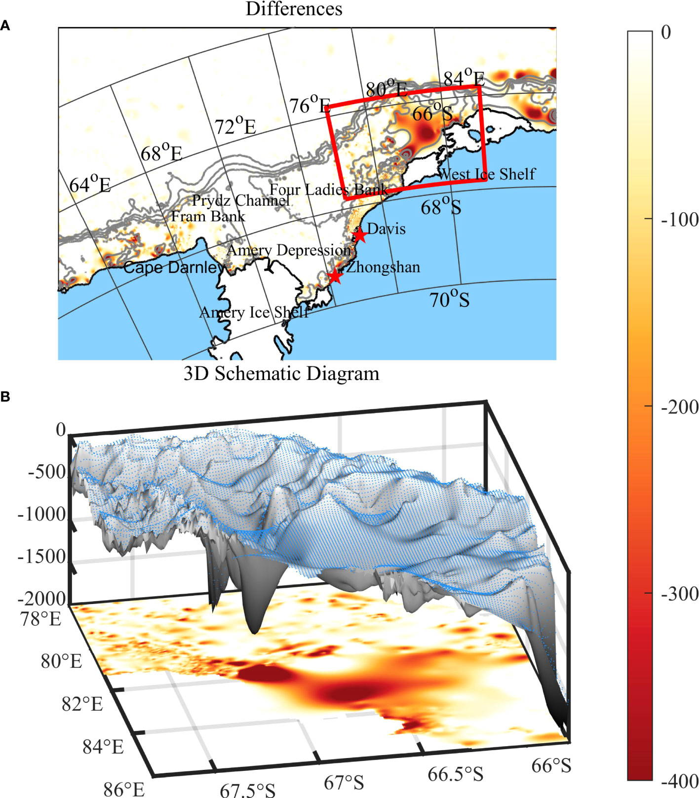
Figure 2 (A) Same as Figure 1B, but for the differences between the CB and IBCSO V1 (CB minus IBCSO V1). (B) The 3D schematic diagram of the bottom topography in the region bounded by the red box in (A). The blue dot represents IBCSO V1, and the grey surface represents the CB. The bottom slice shows the bathymetry differences, which are consistent with (A).
2.3 Model description
In this study, the Massachusetts Institute of Technology General Circulation Model was employed (Marshall et al., 1997), coupling with a sea ice model (Zhang and Hibler III, 1997) and an ice shelf model (Losch et al., 2010). The initial conditions and parameter settings are the same as in the previous version (Liu et al., 2017; Liu et al., 2018). Between the western (60°E) and eastern (90°E) boundaries, the constant meridional grid spacing is ~1.5 km, while the zonal grid spacing decreases from ~2.2 km at the northern boundary (65°S) to ~1.4 km at the southern boundary (74°S). The vertical intervals range from 10 m at the surface to 250 m at the bottom with 70 levels. The Amery Ice Shelf (AIS) and the WIS were represented by a static and thermodynamically active ice shelf in Prydz Bay. The Japanese Re-Analysis (JRA-25) was used to force the ocean and the sea ice components from 1979, including the downward longwave and shortwave radiation, precipitation, 2 m humidity, 2 m air temperature, and 10 m surface wind. This model was integrated for 12 years, and its 5-day mean output was saved. Unless otherwise specified, the analysis was performed using the last 5-year averaging period. Note that this model does not include the frazil ice and tidal processes.
With the same model configuration, two sensitivity simulations were conducted. The first experiment, denoted by Result A, uses RTopo-2 as the bathymetry. The second one using CB as the bathymetry is denoted by Result B. The model performance was evaluated in previous studies (Liu et al., 2017; Liu et al., 2018). The CB in Result B is quite different from RTopo-2 in Result A, and we focus on the dynamic response of the circulation, heat transport, and the AIS basal melting to the bathymetric changes from RTopo-2 to CB in Prydz Bay.
3 Results
3.1 Circulation and temperature fields
The depth-averaged currents in the two experiments (Result A and Result B) are shown in Figure 3. There are two main circulations in Prydz Bay. One is the cyclonic Prydz Bay Gyre (PBG), with its eastern branch responsible for mCDW intrusion and the western branch transporting the shelf water offshore. The other one is the PBECC (Liu et al., 2017; Liu et al., 2018), originating on the eastern side of the FLB and flowing westward along the coastal line (Liu et al., 2017). Importantly, the PBECC just flows around the southeast side of the FLB where the largest bathymetric change occurs in the CB (Figure 2B). Therefore, the significant deepening in CB may exert profound influences on the PBECC (Figure 3).
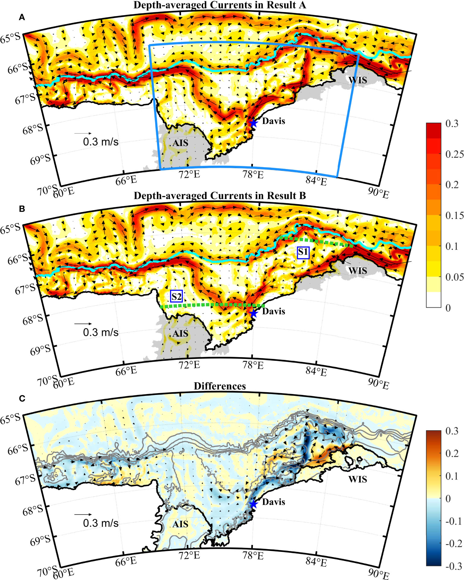
Figure 3 (A) The speeds (m s-1) (color shading) and vectors of the depth-averaged currents in Result A. (B) Same as (A), but for Result B. (C) The differences between Result A and Result B (B minus A). The heat transport within the region bounded by the light blue box (including only the continental shelf and parts of the sub-ice-shelf cavities) in (A) is shown in Figure 6. In (B), the cross-sections (green dashed line) where the heat transports are shown in Figure 7 are labelled by S1 (66.1°S) and S2 (68.3°S), respectively. The semitransparent regions denote the AIS and the WIS. The solid black lines are the coastlines and the ice-shelf fronts. The grey lines are bathymetric contours in CB, with 500 m intervals from 500 m to 2000 m depth. The cyan line are 1000 m bathymetric contours in CB.
In Result A, the PBECC originates from the shelf break, with two main sources (Figure 3A). One is located at the shelf break of 82°E and flows southward. The other one originates at the shelf break near 90°E and flows westward on the north of the WIS calving front. These two branches merge together at ~67°S and head towards the Davis Station (Figure 3A). In contrast, in the simulation with the CB (Result B), there is only one origin of the PBECC, which is close to the shelf break near 90°E. The PBECC in Result B still flows along the WIS calving front towards the Davis Station, but with obviously stronger transport than in Result A (Figure 3B). As the PBECC passes through 67°S, a small fraction of the PEBCC reverses to the north. This is consistent with the remarkable deepening of the seabed to the north of the WIS in CB. To conserve the potential vorticity, the deepening of the ocean bottom in this area generates a cyclonic circulation due to the stretching of the water column. Along the coastal line from the WIS to the eastern AIS calving front, the flow speed in Result B is slower than in Result A (Figure 3C), and the large differences can be up to 0.2 m s-1 from the west side of the WIS to the Davis Station.
The changes in the circulation also result in substantial changes in the potential temperature and salinity fields. We distinguish the shelf from the deep ocean by the 1000 m isobath. The differences of the potential temperature on the shelf between Result A and Result B are shown in Figure 4A. Over the continental shelf, the depth-averaged potential temperature becomes colder over the FLB and the Amery Depression, while the potential temperature is warmer to the southeast of the FLB. The maximum potential temperature decrease can be lower than -0.1°C. The spatial pattern of the salinity differences is generally opposite to that of the potential temperature, with the salinity increase (decrease) corresponding to the potential temperature decrease (increase), except in the north of the WIS. The large changes in the potential temperature and salinity indicate that the circulation changes induced by the differences between RTopo-2 and CB can result in remarkable influences on the simulated water properties.
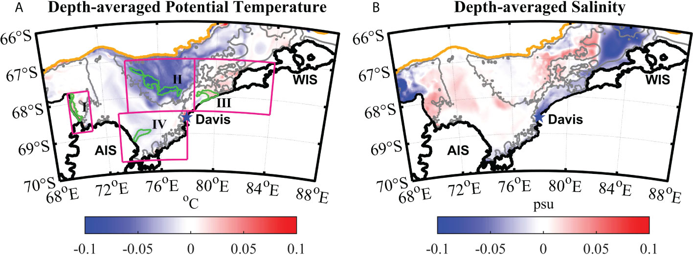
Figure 4 (A) The differences of the depth-averaged potential temperature (°C) between Result A and Result B (B minus A). The green wireframes indicate the locations where the potential temperature changes are the greatest within the specified regions (I, II, III, and IV) bounded by the pink boxes. The grey line and the orange line represent the 500 m and 1000 m isobaths from the CB, respectively. (B) Same as (A), but for the salinity (psu).
To illustrate the changes in the vertical structures of the potential temperature and salinity, the potential temperature and salinity profiles with large potential temperature changes in the selected regions in Figure 4A are shown in Figure 5.
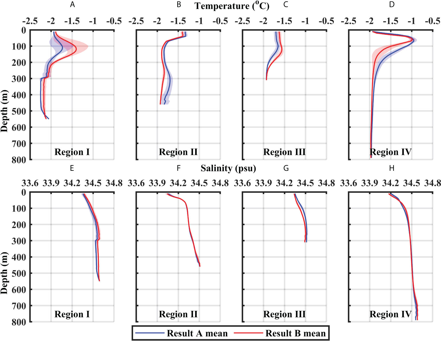
Figure 5 (A–D) The potential temperature profiles (°C) of Result A (blue) and Result B (red) in Regions I, II, III, and IV shown by the green wireframes in Figure 4A (dark color: mean of all profiles; light color: the ranges of one standard deviation above and below the mean values). (E–H) Same as (A–D), but for the salinity profiles (psu).
The potential temperature profiles in Results B in the four regions differ considerably from those in Result A, and so are the salinity profiles in Regions I and III. In Regions II and IV, significant cooling has been identified in the potential temperature profiles. The potential temperature in Region II cools greatly in the lower layer from the water depth of 100m to the seabed, and the maximum difference even exceeds 0.2°C. Region II is located over the FLB, and the potential temperature profiles in this region show that the potential temperature in Results B below 100 m depth is lower than that in Results A, which indicates that mCDW intrusion over the FLB decreases due to the bathymetry correction. Region IV is located downstream of the PBECC, and the strong potential temperature cooling from Result A to Result B at 80-300 m depths can be seen in Figure 5D. The temperature profiles in Region IV show that the potential temperature of the water mass close to the eastern AIS calving front decreases significantly in Result B, implying that the heat delivered into the AIS cavity may also decrease.
There are also obvious changes in the vertical structures of the potential temperature in Regions I and III where the depth-averaged potential temperature warms up in Result B. Region III is just located in the area where the bathymetry correction is large. The large deepening of the seabed in Region III and its northeastern flank results in warming in the entire water column, coinciding with the intensified PEBCC in Result B. By comparisons between results A and B, although both the temperature in Region I and Region III increased, the salinity changes were not the same. The salinity in Region I increases, but the salinity in Region III decreases.
3.2 Heat transport
The changes in the circulations and water mass properties can induce changes in the heat transport towards the AIS front. To quantify the influences of the bathymetry correction on the heat delivered into the sub-ice-shelf cavities, we calculate the meridional heat transport across every zonal cross-section within the box shown in Figure 4B. Both the net heat transport and the southward heat transport (calculated by using the southward meridional velocity only) are calculated. As shown in Figure 6, the net heat transport is much smaller than the southward heat transport, owing to the cancellation between the northward outflow and the southward inflow. The most notable feature is the relatively large changes in the southward heat transport over the latitude band of 66°S-67.2°S (the dashed lines in Figure 6A and the pink line in Figure 6B). Figure 6B shows a positive peak of the differences of the southward heat transport at ~66.1°S (the southward heat transport reduces from ~5.23×10¹³ J s-1 to ~4.07×10¹³ J s-1, by ~22.18%), while a negative peak appears around ~66.7°S (an increasing from ~5.48×10¹³ J s-1 to ~6.87×10¹³ J s-1, by ~25.37%). Such relatively large changes in the southward heat transport within the latitude band of 66°S - 67.2°S are closely related to the significant changes in the circulation in the eastern Prydz Bay. The third peak occurs at ~68.3°S, where the southward heat transport reduces from ~5.95×10¹³ J s-1 to ~4.87×10¹³ J s-1, by ~18.15%. Overall, Result B shows a weakened southward heat transport over the continental shelf. Therefore, the bathymetry correction leads to reduced heat transport towards the AIS front, which may also reduce the basal melting of the AIS.
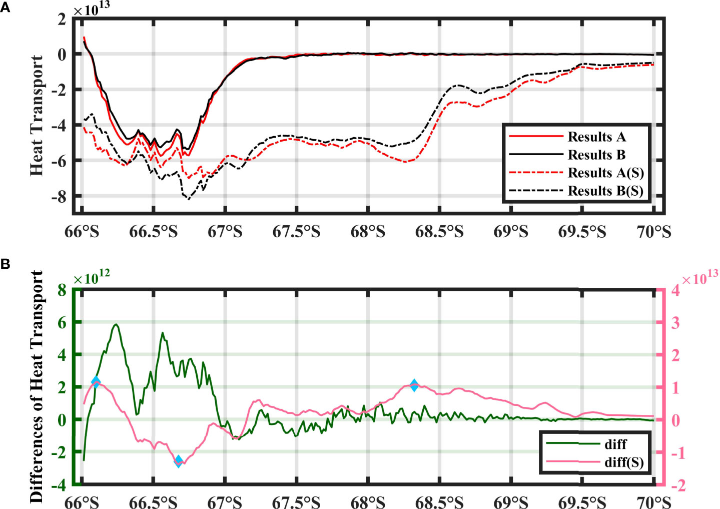
Figure 6 (A) The zonally integrated meridional heat transport (J s-1) (negative is southward) across every zonal cross-section within the light blue box in Figure 3A. The solid red (black) line indicates the net heat transport in Result A (Result B). The dashed lines (S) are the same as the solid lines, but for the heat transport calculated by only using the southward velocity. (B) same as (A), but for the differences between Result A and Result B (B minus A). The three blue diamond marks denote the three peaks at the latitudes of 66.1°S, 66.7°S and 68.3°S, respectively.
To examine the changes in the heat transports in detail, the heat transports at two cross-sections (see S1 and S2 in Figure 3B) where the two peak values occur are shown in Figure 7. The zonal extension of the northward heat transport across 66.1°S in Result B becomes obviously widened, and the magnitude of the southward heat transport also decreases (Figures 7A–C), leading to the reduced southward heat transport towards the AIS front. These changes in the heat transport are dominated by the changes in the circulation. For example, the enhanced northward heat transport at 82.5°E is caused by the local intensified northward flow. At the cross-section S2 (68.3°S) close to the AIS calving front, the magnitude of the meridional velocity on the eastern side decreases (Figure 3C), resulting in the decrease in both the southward and the northward heat transport (Figures 7D–F). The spatial pattern of the meridional heat transport at this cross-section has not changed much between Result A and Result B, and thus the decrease in the southward heat transport is mainly induced by the slowing down of the southward velocity.
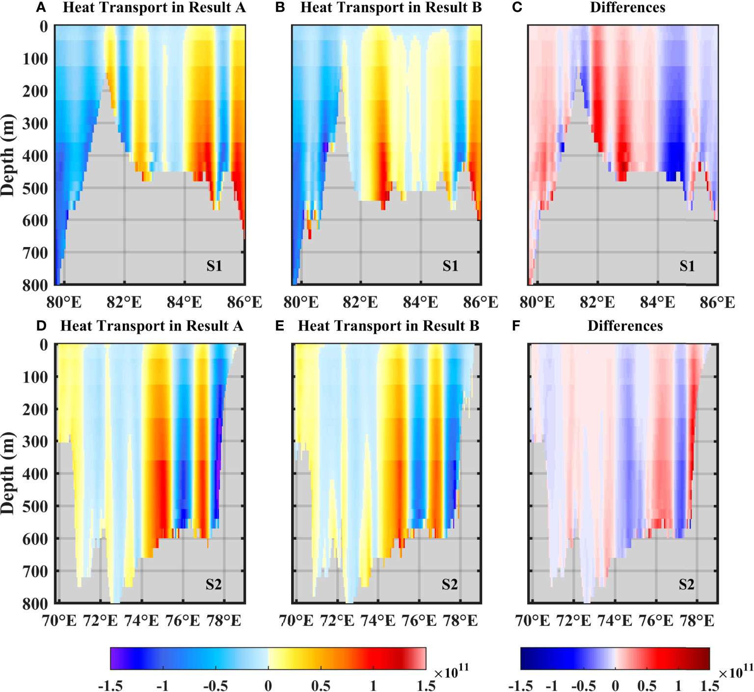
Figure 7 The heat transport (J s-1) cross-section at 66.1°S (S1) and 68.3°S (S2) (negative is southward). (A, D) Result A; (B, E) Result B; (C, F) The differences between Result A and Result B (B minus A). The locations of cross-sections S1 and S2 are shown in Figure 3B.
3.3 Basal melting of Amery Ice Shelf
Result A and Result B both capture the highest melting rate near the grounding line of the AIS, with refreezing in the northwestern flank and melting in the southeastern flank (Figures 8A, B), which is consistent with previous studies (Galton‐Fenzi et al., 2012; Herraiz-Borreguero et al., 2015; Liu et al., 2017).
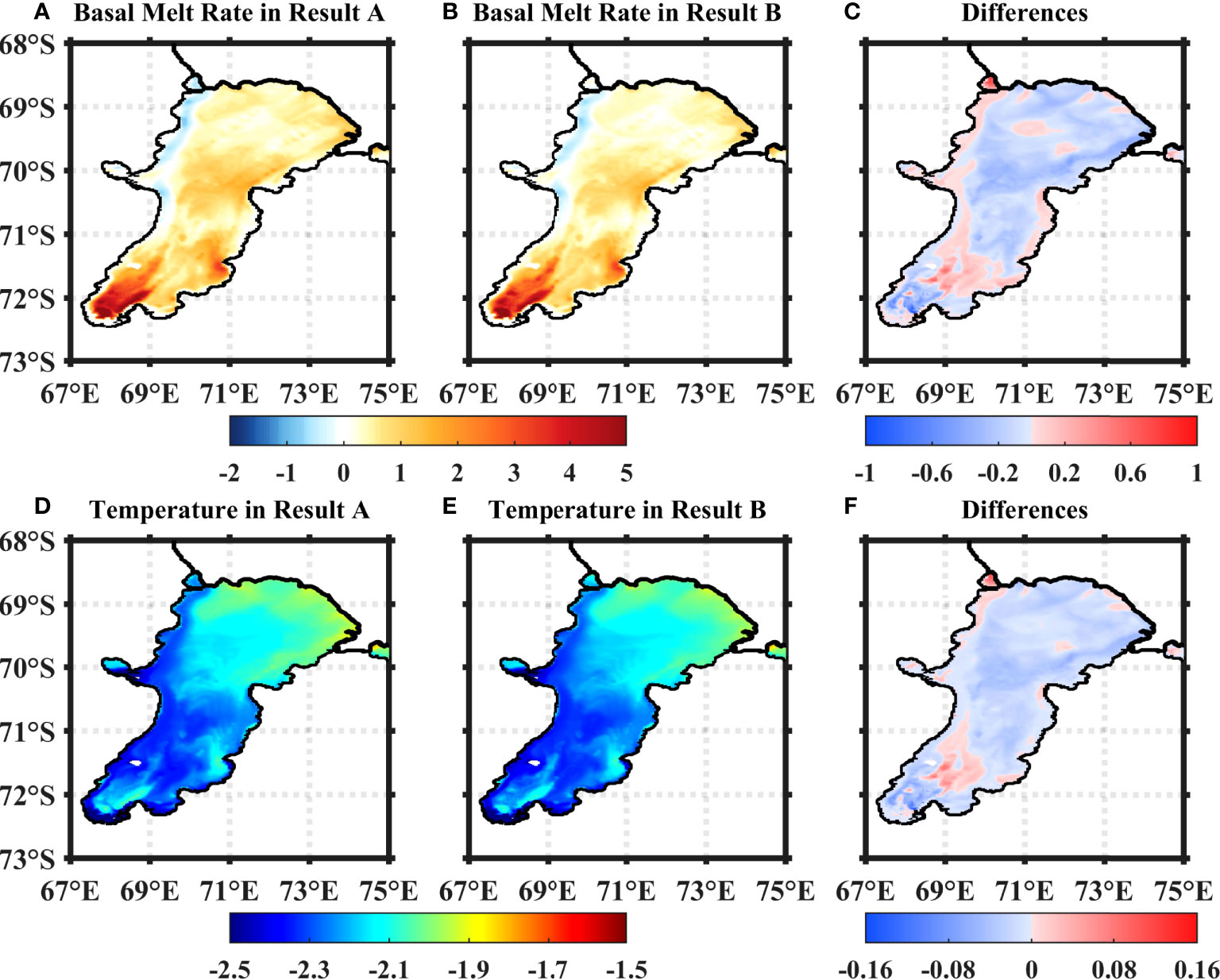
Figure 8 The basal melt rate (m yr-1, melting is positive) of the AIS in (A) Result A and (B) Result B. The solid black lines are the coastline, the grounding line, and the AIS calving front. (C) The differences between Result A and Result B (A, B). (D–F) Same as (A–C), but for the potential temperature (°C) of the layer adjacent to the AIS basal surface.
Figure 8C shows the differences of basal melting between the two experiments. Result B shows decreasing melting rate in the broad melting region beneath the AIS, and there is also decreasing refreezing rate in the freezing region in the western flank. Overall, Result B shows a lower basal melting rate and refreezing rate than that in Result A. Compared with Result A, the net basal melting rate in Result B reduces by ~13.04% (Table 1), with a maximum decrease of ~1 m yr-1 at the grounding line (Figure 8C). Figures 8D–F shows the temperature of the layer adjacent to the base of the AIS and the difference between Result A and Result B. In the eastern flank, the middle region, and near the grounding line of the AIS, the water in Result B is colder than that in Result A. Near 71.5°S, the water is warmer in Result B than in Result A.
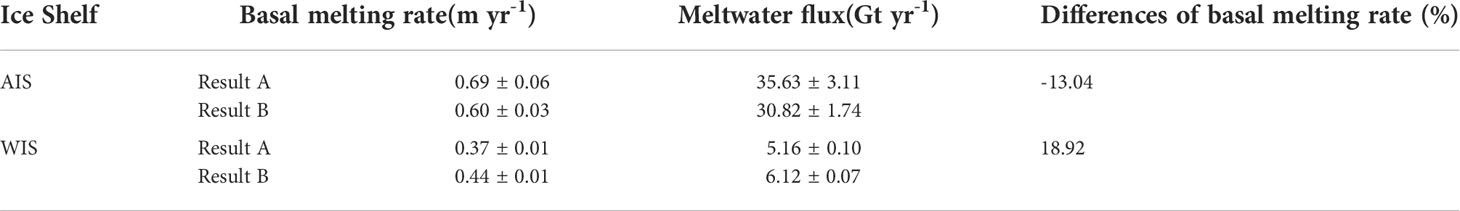
Table 1 Basal melting rate (in m yr-1), meltwater flux (in Gt yr-1), and the changes of basal melting rate (in %) of the ice shelves between result A and result B (B minus A, plus or minus: the ranges of one standard deviation above and below the mean values).
Compared with Result A, the reduction of the southward warm water transport in Result B leads to the reduction of heat transport into the sub-ice-shelf cavity of the AIS, which results in a lower basal melting rate. Due to the warmer potential temperature in the cavity of the WIS in Result B than in Result A, the basal melting of the WIS is enhanced in Result B (not shown). The basal melt rate of the WIS increases by ~18.92% (Table 1). Since the geometry of the sub-ice-shelf cavity has not been changed in this study, the changes of the basal melting change are only induced by the bathymetry correction over the continental shelf. This result suggests that the basal melting rate of the AIS in previous modelling studies (Galton‐Fenzi et al., 2012; Liu et al., 2017; Liu et al., 2018) might still have some uncertainties associated with the potential deficiency in the adopted bathymetry of Prydz Bay.
4 Summary and discussion
The bathymetry of Prydz Bay in IBCSO V1 was recently optimized by introducing the water depth data from various hydrographic observations (Tao et al., 2021). In particular, the seafloor adjacent to the north of the WIS front deepens considerably, resulting in a large and wide depression to the east of the Four Lady Bank (FLB). Unlike the relatively smooth seafloor morphology of this region in IBCSO V1 and RTopo-2, the corrected bathymetry (CB) shows a more refined and irregular morphology.
To study the influences of the large changes in the bathymetry on the circulations and the basal melting/freezing of the ice shelves, we conducted two sensitivity experiments by using a regional coupled ocean-sea ice-ice shelf model (Liu et al., 2017; Liu et al., 2018): one uses the original RTopo-2, and the other one uses the CB for the continental shelf region. Due to the differences between the two bathymetry datasets, the simulated circulations over the eastern region of Prydz Bay are significantly different between the two experiments. The most notable differences are the changes of the source region of the PBECC, along with the decrease of its strength downstream. These changes are mainly caused by the large deepening of the seabed over the eastern region of Prydz Bay.
Associated with the changes in the circulation, the changes in the bathymetry also cause significant changes in the water mass properties in Prydz Bay. The most remarkable influence is that the CB leads to generally colder potential temperature in Prydz Bay. The reason is that the Antarctic Slope Current near the FLB is weakened by the changes from upstream, resulting in less mCDW intrusion over the FLB (Liu et al., 2018). While an increase in the potential temperature can be seen to the north of the WIS front, the potential temperature downstream close to the AIS front cools down due to the slowing down of the PEBCC downstream. The widespread cooling in the potential temperature near the AIS calving front also indicates the decrease in the southward heat transport.
Our model results show that the basal melting of the AIS is broadly reduced due to the bathymetry correction, while the enhanced refreezing can also be seen in the western flank of the AIS. The reduced basal melting mainly results from the cooling of the water layer adjacent to the base of the AIS. The total basal melting of the AIS decreases from ~35.63 Gt yr-1 to ~30.82 Gt yr-1, by ~13.50%. The increased potential temperature at locations upstream of the PBECC also exposes the WIS cavity to relatively warmer water, which increases the basal melting of the WIS. Therefore, in contrast to the AIS, the total basal melting of the WIS increases from ~5.16 Gt yr-1 to ~6.12 Gt yr-1, by ~18.60%.
We note that the shelf circulations and the ice shelf basal melting should be affected by more factors than the shelf bathymetry, such as the geometry of the sub-ice-shelf cavities (Yang et al., 2021), the drifting and grounding icebergs (Dinniman et al., 2007; Cougnon et al., 2017; Hou and Shi, 2021), and the distribution of fast ice (Fraser et al., 2021). With a focus on the effects of the bathymetry changes on the shelf circulations and the ice shelf basal melting, this study is an important first step towards a comprehensive understanding of the effects of such various factors. Since giant icebergs can have a lifetime of several decades and can exert great effects on the distribution of fast ice and polynyas, we call for the development of an iceberg module and a fast ice module that can realistically simulate the corresponding thermodynamic and dynamic processes. In the future, a more realistic coupled ocean-sea ice-ice shelf model should at least include these two modules and should employ more reliable shelf bathymetry and the geometry of the sub-ice-shelf cavities, in addition to other improvements.
Data availability statement
The data used to reproduce these figures in this manuscript can be found below: https://pan.baidu.com/s/1h2Ci9s7SZyXYXv-I1Lsvw (code: 4567). The corrected bathymetry and model outputs used in this study are available upon request (bGl1Y2hlbmd5YW5Ac21sLXpodWhhaS5jbg== and emhhb21pbi53YW5nQGhodS5lZHUuY24=).
Author contributions
CS performed the model simulation and data analyses and wrote the manuscript. CL and ZW were behind the ideas of the study, and revised the manuscript. LY contributed to the data analysis and model simulation. YT provided the corrected bathymetry data. QQ and JQ provided technical support and improved the manuscript. All authors contributed to the article and approved the submitted version.
Funding
This work was supported by the National Natural Science Foundation of China (NSFC) Projects (Nos: 41941007; 41876220), by the Innovation Group Project of Southern Marine Science and Engineering Guangdong Laboratory (Zhuhai) (No. 311021008), by the Independent Research Foundation of Southern Marine Science and Engineering Guangdong Laboratory (Zhuhai) (SML2021SP306).
Acknowledgments
The RTopo-2 data are available through the PANGAEA Data Publisher for Earth & Environmental Science (https://doi.pangaea.de/10.1594/PANGAEA.856844). IBCSO V1 are publically available from the IBCSO homepage (www.ibcso.org) and at http://dx.doi.org/10.1594/PANGAEA.805736. The MITgcm code was obtained freely from http://mitgcm.org/.
Conflict of interest
The authors declare that the research was conducted in the absence of any commercial or financial relationships that could be construed as a potential conflict of interest.
Publisher’s note
All claims expressed in this article are solely those of the authors and do not necessarily represent those of their affiliated organizations, or those of the publisher, the editors and the reviewers. Any product that may be evaluated in this article, or claim that may be made by its manufacturer, is not guaranteed or endorsed by the publisher.
References
Adusumilli S., Fricker H. A., Medley B., Padman L., Siegfried M. R. (2020). Interannual variations in meltwater input to the southern ocean from Antarctic ice shelves. Nat. Geosci. 13, 616–620. doi: 10.1038/s41561-020-0616-z
Arndt J. E., Schenke H. W., Jakobsson M., Nitsche F. O., Buys G., Goleby B., et al. (2013). The international bathymetric chart of the southern ocean (IBCSO) version 1.0–a new bathymetric compilation covering circum-Antarctic waters. Geophys. Res. Lett. 40, 3111–3117. doi: 10.1002/grl.50413
Barthélemy A., Goosse H., Fichefet T., Lecomte O. (2018). On the sensitivity of Antarctic sea ice model biases to atmospheric forcing uncertainties. Climate Dynamics 51, 1585–1603. doi: 10.1007/s00382-017-3972-7
Beaman R. J., O’Brien P. E., Post A. L., De Santis L. (2011). A new high-resolution bathymetry model for the Terre adélie and George V continental margin, East Antarctica. Antarctic Sci. 23, 95–103. doi: 10.1017/S095410201000074X
Becker J., Sandwell D., Smith W., Braud J., Binder B., Depner J., et al. (2009). Global bathymetry and elevation data at 30 arc seconds resolution: SRTM30_PLUS. Mar. Geodesy 32, 355–371. doi: 10.1080/01490410903297766
Brodeau L., Barnier B., Treguier A.-M., Penduff T., Gulev S. (2010). An ERA40-based atmospheric forcing for global ocean circulation models. Ocean Model. 31, 88–104. doi: 10.1016/j.ocemod.2009.10.005
Cochran J. R., Tinto K. J., Bell R. E. (2020). Detailed bathymetry of the continental shelf beneath the getz ice shelf, West Antarctica. J. Geophys. Research: Earth Surface 125, e2019JF005493. doi: 10.1029/2019JF005493
Cougnon E., Galton-Fenzi B., Rintoul S., Legrésy B., Williams G., Fraser A., et al. (2017). Regional changes in icescape impact shelf circulation and basal melting. Geophys. Res. Lett. 44, 11,519–511,527. doi: 10.1002/2017GL074943
Daae K., Hattermann T., Darelius E., Mueller R. D., Naughten K. A., Timmermann R., et al. (2020). Necessary conditions for warm inflow toward the filchner ice shelf, weddell Sea. Geophys. Res. Lett. 47, e2020GL089237. doi: 10.1029/2020GL089237
Dickens W. A., Graham A. G., Smith J. A., Dowdeswell J. A., Larter R. D., Hillenbrand C. D., et al. (2014). A new bathymetric compilation for the south Orkney islands region, Antarctic peninsula (49–39 W to 64–59 s): Insights into the glacial development of the continental shelf. Geochem. Geophys. Geosy. 15, 2494–2514. doi: 10.1002/2014GC005323
Dinniman M. S., Klinck J. M., Smith W. O. Jr (2007). Influence of sea ice cover and icebergs on circulation and water mass formation in a numerical circulation model of the Ross Sea, Antarctica. J. Geophys. Research: Oceans 112, C11013. doi: 10.1029/2006JC004036
Dupont T., Alley R. (2005). Assessment of the importance of ice-shelf buttressing to ice-sheet flow. Geophys. Res. Lett. 32, L04503. doi: 10.1029/2004GL022024
Eisermann H., Eagles G., Ruppel A. S., Läufer A., Jokat W. (2021). Bathymetric control on borchgrevink and roi baudouin ice shelves in East Antarctica. J. Geophys. Research: Earth Surface 126, e2021JF006342. doi: 10.1029/2021JF006342
Fraser A. D., Massom R. A., Handcock M. S., Reid P., Ohshima K. I., Raphael M. N., et al. (2021). Eighteen-year record of circum-Antarctic landfast-sea-ice distribution allows detailed baseline characterisation and reveals trends and variability. Cryosphere 15, 5061–5077. doi: 10.5194/tc-15-5061-2021
Fretwell P., Pritchard H. D., Vaughan D. G., Bamber J. L., Barrand N. E., Bell R., et al. (2013). Bedmap2: improved ice bed, surface and thickness datasets for Antarctica. Cryosphere 7, 375–393. doi: 10.5194/tc-7-375-2013
Galton-Fenzi B., Hunter J., Coleman R., Marsland S., Warner R. (2012). Modeling the basal melting and marine ice accretion of the amery ice shelf. J. Geophys. Research: Oceans 117, C09031. doi: 10.1029/2012JC008214
GEBCO Bathymetric Compilation Group (2019). The GEBCO_2019 grid-a continuous terrain model of the global oceans and land (UK: British Oceanographic Data Centre, National Oceanography Centre, NERC).
Goldberg D. N., Smith T. A., Narayanan S. H., Heimbach P., Morlighem M. (2020). Bathymetric influences on Antarctic ice-shelf melt rates. J. Geophys. Research: Oceans 125, e2020JC016370. doi: 10.1029/2020JC016370
Graham A. G., Nitsche F., Larter R. D. (2011). An improved bathymetry compilation for the bellingshausen Sea, Antarctica, to inform ice-sheet and ocean models. Cryosphere 5, 95–106. doi: 10.5194/tc-5-95-2011
Griffiths S. D., Peltier W. R. (2009). Modeling of polar ocean tides at the last glacial maximum: Amplification, sensitivity, and climatological implications. J. Climate 22, 2905–2924. doi: 10.1175/2008JCLI2540.1
Hellmer H. H., Kauker F., Timmermann R., Determann J., Rae J. (2012). Twenty-first-century warming of a large Antarctic ice-shelf cavity by a redirected coastal current. Nature 485, 225–228. doi: 10.1038/nature11064
Herraiz-Borreguero L., Coleman R., Allison I., Rintoul S. R., Craven M., Williams G. D. (2015). Circulation of modified circumpolar deep water and basal melt beneath the amery ice shelf, East a ntarctica. J. Geophys. Research: Oceans 120, 3098–3112. doi: 10.1002/2015JC010697
Herraiz-Borreguero L., Lannuzel D., van der Merwe P., Treverrow A., Pedro J. (2016). Large Flux of iron from the amery ice shelf marine ice to prydz bay, East Antarctica. J. Geophys. Research: Oceans 121, 6009–6020. doi: 10.1002/2016JC011687
Hooker S. K., Boyd I. L. (2003). Salinity sensors on seals: use of marine predators to carry CTD data loggers. Deep Sea Res. Part I: Oceanogr. Res. Papers 50, 927–939. doi: 10.1016/S0967-0637(03)00055-4
Hou S., Shi J. (2021). Variability and formation mechanism of polynyas in Eastern prydz bay, Antarctica. Remote Sens. 13, 5089. doi: 10.3390/rs13245089
Large W., Danabasoglu G. (2006). Attribution and impacts of upper-ocean biases in CCSM3. J. Climate 19, 2325–2346. doi: 10.1175/JCLI3740.1
Liu Y., Moore J. C., Cheng X., Gladstone R. M., Bassis J. N., Liu H., et al. (2015). Ocean-driven thinning enhances iceberg calving and retreat of Antarctic ice shelves. Proc. Natl. Acad. Sci. 112, 3263–3268. doi: 10.1073/pnas.1415137112
Liu C., Wang Z., Cheng C., Wu Y., Xia R., Li B., et al. (2018). On the modified circumpolar deep water upwelling over the four ladies bank in prydz bay, East Antarctica. J. Geophys. Research: Oceans 123, 7819–7838. doi: 10.1029/2018JC014026
Liu C., Wang Z., Cheng C., Xia R., Li B., Xie Z. (2017). Modeling modified circumpolar deep water intrusions onto the prydz bay continental shelf, East Antarctica. J. Geophys. Research: Oceans 122, 5198–5217. doi: 10.1002/2016JC012336
Losch M., Menemenlis D., Campin J.-M., Heimbach P., Hill C. (2010). On the formulation of sea-ice models. part 1: Effects of different solver implementations and parameterizations. Ocean Model. 33, 129–144. doi: 10.1016/j.ocemod.2009.12.008
Makinson K., Holland P. R., Jenkins A., Nicholls K. W., Holland D. M. (2011). Influence of tides on melting and freezing beneath filchner-ronne ice shelf, Antarctica. Geophys. Res. Lett. 38, L06601. doi: 10.1029/2010GL046462
Marshall J., Adcroft A., Hill C., Perelman L., Heisey C. (1997). A finite-volume, incompressible navier stokes model for studies of the ocean on parallel computers. J. Geophys. Research: Oceans 102, 5753–5766. doi: 10.1029/96JC02775
Mayer L., Jakobsson M., Allen G., Dorschel B., Falconer R., Ferrini V., et al. (2018). The Nippon foundation–GEBCO seabed 2030 project: The quest to see the world’s oceans completely mapped by 2030. Geosciences 8, 63. doi: 10.3390/geosciences8020063
McConnell B., Chambers C., Fedak M. (1992). Foraging ecology of southern elephant seals in relation to the bathymetry and productivity of the southern ocean. Antarctic Sci. 4, 393–398. doi: 10.1017/S0954102092000580
Millan R., Rignot E., Bernier V., Morlighem M., Dutrieux P. (2017). Bathymetry of the amundsen Sea embayment sector of West Antarctica from operation IceBridge gravity and other data. Geophys. Res. Lett. 44, 1360–1368. doi: 10.1002/2016GL072071
Millan R., St-Laurent P., Rignot E., Morlighem M., Mouginot J., Scheuchl B. (2020). Constraining an ocean model under getz ice shelf, Antarctica, using a gravity-derived bathymetry. Geophys. Res. Lett. 47, e2019GL086522. doi: 10.1029/2019GL086522
Nakayama Y., Manucharyan G., Zhang H., Dutrieux P., Torres H. S., Klein P., et al. (2019). Pathways of ocean heat towards pine island and thwaites grounding lines. Sci. Rep. 9, 1–9. doi: 10.1038/s41598-019-53190-6
Nicholls K. W., Østerhus S., Makinson K., Gammelsrød T., Fahrbach E. (2009). Ice-ocean processes over the continental shelf of the southern weddell Sea, Antarctica: A review. Rev. Geophys. 47, RG3003. doi: 10.1029/2007RG000250
Nitsche F., Jacobs S., Larter R., Gohl K. (2007). Bathymetry of the amundsen Sea continental shelf: Implications for geology, oceanography, and glaciology. Geochem. Geophys. Geosy. 8, Q10009. doi: 10.1029/2007GC001694
Nitsche F., Porter D., Williams G., Cougnon E., Fraser A., Correia R., et al. (2017). Bathymetric control of warm ocean water access along the East Antarctic margin. Geophys. Res. Lett. 44, 8936–8944. doi: 10.1002/2017GL074433
Padman L., Costa D. P., Bolmer S. T., Goebel M. E., Huckstadt L. A., Jenkins A., et al. (2010). Seals map bathymetry of the Antarctic continental shelf. Geophys. Res. Lett. 37, L21601. doi: 10.1029/2010GL044921
Padman L., Fricker H. A., Coleman R., Howard S., Erofeeva L. (2002). A new tide model for the Antarctic ice shelves and seas. Ann. Glaciology 34, 247–254. doi: 10.3189/172756402781817752
Padman L., Siegfried M. R., Fricker H. A. (2018). Ocean tide influences on the Antarctic and Greenland ice sheets. Rev. Geophys. 56, 142–184. doi: 10.1002/2016RG000546
Pritchard H., Ligtenberg S. R., Fricker H. A., Vaughan D. G., van den Broeke M. R., Padman L. (2012). Antarctic Ice-sheet loss driven by basal melting of ice shelves. Nature 484, 502–505. doi: 10.1038/nature10968
Reese R., Gudmundsson G. H., Levermann A., Winkelmann R. (2018). The far reach of ice-shelf thinning in Antarctica. Nat. Climate Change 8, 53–57. doi: 10.1038/s41558-017-0020-x
Ribic C. A., Chapman E., Fraser W. R., Lawson G. L., Wiebe P. H. (2008). Top predators in relation to bathymetry, ice and krill during austral winter in Marguerite bay, Antarctica. Deep Sea Res. Part II: Topical Stud. Oceanogr. 55, 485–499. doi: 10.1016/j.dsr2.2007.11.006
Rignot E., Jacobs S. S. (2002). Rapid bottom melting widespread near Antarctic ice sheet grounding lines. Science 296, 2020–2023. doi: 10.1126/science.1070942
Rignot E., Jacobs S., Mouginot J., Scheuchl B. (2013). Ice-shelf melting around Antarctica. Science 341, 266–270. doi: 10.1126/science.1235798
Rosier S., Green J., Scourse J., Winkelmann R. (2014). Modeling Antarctic tides in response to ice shelf thinning and retreat. J. Geophys. Research: Oceans 119, 87–97. doi: 10.1002/2013JC009240
Sandwell D. T., Smith W. H. (2001). Bathymetric estimation. Int. Geophys. Elsevier 69, 441–457. doi: 10.1016/S0074-6142(01)80157-1
Schaffer J., Timmermann R., Arndt J. E., Kristensen S. S., Mayer C., Morlighem M., et al. (2016). A global, high-resolution data set of ice sheet topography, cavity geometry, and ocean bathymetry. Earth System Sci. Data 8, 543–557. doi: 10.5194/essd-8-543-2016
Smith J., Nogi Y., Spinoccia M., Dorschel B., Leventer A. (2021). A bathymetric compilation of the cape darnley region, East Antarctica. Antarctic Sci. 33, 548–559. doi: 10.1017/S0954102021000298
Stewart A. L., Klocker A., Menemenlis D. (2018). Circum-Antarctic shoreward heat transport derived from an eddy-and tide-resolving simulation. Geophys. Res. Lett. 45, 834–845. doi: 10.1002/2017GL075677
Tao Y., Liu C., Wang Z. (2021). An improved digital bathymetric model for prydz bay by hydrography observations. Trans. Atmospheric Sci. 44, 128–139. doi: 10.13878/j.cnki.dqkxxb.20200928001
Thoma M., Jenkins A., Holland D., Jacobs S. (2008). Modelling circumpolar deep water intrusions on the amundsen Sea continental shelf, Antarctica. Geophys. Res. Lett. 35, L18602. doi: 10.1029/2008GL034939
Timmermann R., Le Brocq A., Deen T., Domack E., Dutrieux P., Galton-Fenzi B., et al. (2010). A consistent data set of Antarctic ice sheet topography, cavity geometry, and global bathymetry. Earth System Sci. Data 2, 261–273. doi: 10.5194/essd-2-261-2010
Tinto K., Padman L., Siddoway C., Springer S., Fricker H., Das I., et al. (2019). Ross Ice shelf response to climate driven by the tectonic imprint on seafloor bathymetry. Nat. Geosci. 12, 441–449. doi: 10.1038/s41561-019-0370-2
Walker D. P., Brandon M. A., Jenkins A., Allen J. T., Dowdeswell J. A., Evans J. (2007). Oceanic heat transport onto the amundsen Sea shelf through a submarine glacial trough. Geophys. Res. Lett. 34, L02602. doi: 10.1029/2006GL028154
Weatherall P., Marks K. M., Jakobsson M., Schmitt T., Tani S., Arndt J. E., et al. (2015). A new digital bathymetric model of the world's oceans. Earth space Sci. 2, 331–345. doi: 10.1002/2015EA000107
Williams G., Herraiz-Borreguero L., Roquet F., Tamura T., Ohshima K., Fukamachi Y., et al. (2016). The suppression of Antarctic bottom water formation by melting ice shelves in prydz bay. Nat. Commun. 7, 1–9. doi: 10.1038/ncomms12577
Yang J., Guo J., Greenbaum J. S., Cui X., Tu L., Li L., et al. (2021). Bathymetry beneath the amery ice shelf, East Antarctica, revealed by airborne gravity. Geophys. Res. Lett. 48, e2021GL096215. doi: 10.1029/2021GL096215
Zaron E. D. (2019). Simultaneous estimation of ocean tides and underwater topography in the weddell Sea. J. Geophys. Research: Oceans 124, 3125–3148. doi: 10.1029/2019JC015037
Keywords: prydz bay, corrected bathymetry, numerical experiments, circulation, heat transport, basal melting
Citation: Sun C, Liu C, Wang Z, Yan L, Tao Y, Qin Q and Qian J (2022) On the influences of the continental shelf bathymetry correction in Prydz Bay, East Antarctica. Front. Mar. Sci. 9:957414. doi: 10.3389/fmars.2022.957414
Received: 08 June 2022; Accepted: 08 August 2022;
Published: 29 August 2022.
Edited by:
Wei Bo Chen, Central Weather Bureau, TaiwanReviewed by:
Kazuya Kusahara, Japan Agency for Marine-Earth Science and Technology (JAMSTEC), JapanArnold L. Gordon, Columbia University, United States
Copyright © 2022 Sun, Liu, Wang, Yan, Tao, Qin and Qian. This is an open-access article distributed under the terms of the Creative Commons Attribution License (CC BY). The use, distribution or reproduction in other forums is permitted, provided the original author(s) and the copyright owner(s) are credited and that the original publication in this journal is cited, in accordance with accepted academic practice. No use, distribution or reproduction is permitted which does not comply with these terms.
*Correspondence: Chengyan Liu, bGl1Y2hlbmd5YW5Ac21sLXpodWhhaS5jbg==; Zhaomin Wang, emhhb21pbi53YW5nQGhodS5lZHUuY24=