The inhibition of warm advection on the southward expansion of sea ice during early winter in the Bering Sea

Recent observations demonstrate that the Bering Sea exhibits a substantial positive trend of sea ice area increment (ΔSIA, difference in SIA between the current and preceding months) in January contrasted to the considerable negative sea ice area (SIA) trend from 1979 to 2020, and the ΔSIA is unrelated to the local wind field anomaly. To better understand the January ΔSIA variability and its physical characteristics, we explore two distinct empirical orthogonal function (EOF) modes of sea ice concentration increments. EOF1 features a reduction in sea ice concentration (SIC) in the south of St. Lawrence Island. EOF2 is characterized by the rise of SIC surrounding St. Lawrence Island. EOF1 is related to the well-known physical process of December strong poleward heat transport in mixed layer depth. During the southward expansion of sea ice, the multiyear variation of the December SST tendency mostly relies on warm advection in the Bering Sea shelf rather than net air-sea heat flux, and the abnormal northeast wind in December no longer plays the role of a dynamic process dominating the ice area expansion, but generates a stronger poleward heat transport in the Bering Sea shelf to inhibit the southward development of sea ice in the later stage. The two physical processes together result in oceanic poleward heat transport regulating the Bering Sea SIA in competition with atmospheric forcing in early winter. Since PC1 (principal component (PC) time series for EOF1) has a high correlation of -0.76 with the maximum SIA in the Bering Sea, it can be used as the prediction index of the Bering Sea maximum SIA.

1 Introduction

The Bering Sea, as one of the marginal seas in the Arctic Ocean, is very different from the Arctic Ocean in terms of its sea ice changes and even exhibits the characteristics of significant oppositional changes (Brown and Arrigo, 2012; Cavalieri and Parkinson, 2012; Stabeno et al., 2012a; Stabeno et al., 2012b; Wu and Chen, 2016). The sea ice cover in the Arctic Ocean exhibited a significant decline in recent years (Parkinson et al., 1999; Parkinson and Cavalieri, 2008; Cavalieri and Parkinson, 2012; Babb et al., 2013; Comiso et al., 2017; Parkinson and DiGirolamo, 2021). Both sea ice area (SIA) and sea ice extent from January–April showed positive trends in the Bering Sea, opposite to the negative trends observed in other Northern Hemisphere regions from 1979 to 2012 (Cavalieri and Parkinson, 2012). Some studies even pointed out that the co-occurrence of sea-ice minima in the Arctic and maxima in the eastern Bering Sea in 2007-2010 suggested a lack of continuity or a ‘decoupling’ between summer sea-ice minima in the Arctic and the subsequent winter/spring sea-ice maxima in the Bering Sea (Stabeno et al., 2012a; de la Vega et al., 2019; Xiao et al., 2020).

Generally, sea ice in the Bering Sea begins to form around the beginning of October and expands southward throughout the winter (Niebauer et al., 1999; Stabeno et al., 2012a; Li et al., 2014). In winter, sea ice forms mainly in the northern coastal area of the Bering Sea and the polynya areas on the southern coast of St. Lawrence Island and is then transported southward by north winds (Alexander and Niebauer, 1981; Niebauer, 1998; Stabeno et al., 2007; Ohshima et al., 2020). With respect to the sea ice generation area, in December, sea ice often occurs north of St. Lawrence Island, while the January SIA increases are more likely to occur in the Bering Sea shelf area (Stabeno et al., 2012a). The large amount of warm water carried by the Bering Sea continental slope current in the southern waters causes a large amount of sea ice to melt, eventually leading to an S-shaped asymmetrical sea ice edge (Niebauer et al., 1999; Li et al., 2014).

Sea ice plays a key role in shaping the ecosystems of the Bering Sea (Kearney et al., 2021). Bering Sea waters contain one of the most productive marine ecosystems in the world and consequently support a large oceanic fishery that is critical for both commercial and subsistence use (Zhang et al., 2010; Hunt et al., 2011; Li et al., 2014; Hunt et al., 2020). Winter ice cover creates a pool of cold bottom water (<2℃) that is protected from summer mixing by the thermocline (Mueter and Litzow, 2008; Stabeno et al., 2012b). The cold pool acts as a cross-shelf migration barrier for subarctic fish species (e.g., walleye pollock and Pacific cod), forcing these fish to remain on the outer shelf and separating them from food sources in the middle shelf and coastal domain (Stabeno et al., 2012b). The extent of ice is also the dominant factor controlling summer conditions for demersal taxa (Mueter and Litzow, 2008). The maximum extent of sea ice and the timing of its retreat in spring also affect where and when sea-ice algae will be available (Hunt et al., 2011; Sigler et al., 2016; Hunt et al., 2020). Understanding the processes that control the temporal evolution of the sea ice distribution is vital for anticipating how the physical-biological system will change in future years and decades (Wang et al., 2012; Alabia et al., 2020).

A conveyor belt mechanism with a northern source, a southern sink, and an intermediate zone where ice is transported southward by northerly winds, has been proposed to explain the basic north–south SIA structure using observations alone (Pease, 1980; Niebauer et al., 1999; Li et al., 2014). In the northern Bering Sea, northerly or northeasterly wintertime winds promote ice growth and favor the southward transport of sea ice, while northward oceanic heat transport from the southern Bering Sea shelf can accelerate sea ice melting and inhibit southward sea ice expansion (Stabeno et al., 2007; Brown and Arrigo, 2012; Li et al., 2014). Simulation results have shown that from January to May, northeasterly winds transport 1.4×10¹² m³ of sea ice to the south. At the same time, the amount of sea ice melted by warm southern waters is 1.5×10¹² m³ (Zhang et al., 2010). The substantial interannual variability in the Bering Sea ice cover is dominated by changes in this combination of the wind-driven ice mass advection and the ocean thermal front at the sea ice edge (Zhang et al., 2010).

The competition between atmospheric forcing and ocean heat transport largely controls the SIA in the Bering Sea. To date, the causes of SIA variabilities in the Bering Sea have been investigated in terms of large-scale atmospheric circulation anomalies (Niebauer, 1988; Nakanowatari et al., 2015), cyclone activity (Screen et al., 2011), local winds (Stabeno and Bell, 2019) and ice influxes driven by northeast winds from the Arctic Ocean (Babb et al., 2013). These studies clearly illustrate the promotion effect of the local wind field on the annual SIA in mid-winter. Cooling at the ice edge and growth/melt in sea ice influence ocean stability and heat transport in the ocean making it difficult to establish a causal relationship between oceanic heat transport and sea-ice extent (Bitz et al., 2005), resulting in less research on the effect of ocean heat transport. Stabeno and Bell (2019) mentioned that sea ice advances are primarily dependent upon atmospheric forcing and, to a smaller degree, on ocean temperatures. In fact, although warm ocean water can delay the advance of ice, persistent cold northerly winds will eventually cool (radiative heat flux and ice melt) the water column sufficiently to push sea ice southward. The inhibition signal of ocean heat transport is probably to be excluded in the interannual variation of SIA in mid-winter. The footprint of the inhibition signal may only be found on an intra-seasonal scale. Li et al. (2014) suggested that it is necessary to evaluate the temporal evolution of SIA anomalies by considering the mean seasonal cycle, including the impacts of anomalous winds, surface energy fluxes, fluctuating currents and mesoscale eddy effects in sea ice research conducted in the Bering Sea. Herein, we present the importance of northward oceanic heat transport of intra-seasonal variability in SIAs in the Bering Sea during early winter in an effort to better understand the factor that contribute to sea ice fluctuations and to address the lack of knowledge regarding the ocean heat transport’s influence on sea ice. Different from previous studies, the paper focuses on the increment of SIA in January, which will be introduced in detail in Section 2.2.1.

This paper is organized into four sections. In Sect. 2, the employed data and methods are described. In Sect. 3, the sea ice concentration increment (ΔSIC) dominance in the Bering Sea in early winter is analyzed, and the first two derived modes are shown to be related to physical processes. Finally, in Sect. 4, the main conclusions are summarized.

2 Materials and methods

2.1 Datasets

Satellite sea ice concentration (SIC) data are employed from the NASA team monthly data derived from the Scanning Multichannel Microwave Radiometer (SMMR) on the Nimbus-7 satellite and from the SSM/I sensors on the DMSP-F8, -F11, and -F13 satellites (Comiso, 2015), with a resolution of 25 km. The temporal range of the dataset is chosen from Jan 1, 1979, to January 31, 2020. The region of interest covers the whole Bering Sea (51-66°N,165-205°E). The SIA is computed as the area weighted by SIC on the grid-cell level and then integrated over the region of interest.

To explore the influence of atmospheric and ocean forcing on sea ice, several satellite remote sensing datasets are used, including sea surface temperature (SST), wind speed at 10 m above the sea surface, and geostrophic current. The SST data used in the paper are from the National Oceanic and Atmospheric Administration (NOAA) optimum interpolation (OI) SST version 2 dataset, a monthly dataset with a resolution of 0.25°×0.25° that is derived from a blend of in situ observations and Advanced Very High-Resolution Radiometer (AVHRR) satellite infrared data. The selected temporal range of this dataset spans from January 1979 to March 2020. Detailed information regarding these data can be found in Rayner et al. (2003).

Wind data at 10 m above mean sea level are acquired from the National Centers for Environmental Prediction/National Center for Atmospheric Research (NCEP/NCAR) reanalysis project conducted in the Earth System Research Laboratory of NOAA (Kalnay et al., 1996). The 2.5° latitude × 2.5° longitude global grid (144×73) data are interpolated to a 0.25°×0.25° grid, which is used to derive the monthly Ekman current, and then, together with geostrophic current, to derive poleward heat transport. January data collected from 1979 to 2020 are selected.

The geostrophic current is computed using the dynamic topography data derived from the Topex/Poseidon and European Remote-sensing Satellite (ERS) altimetric. The resolution of these data is 0.25°×0.25°, and detailed information characterizing these data can be acquired from the AVISO database (https://www.aviso.altimetry.fr/).

The diagnostic results obtained from the Estimating the Circulation and Climate of the Ocean, Phase II (ECCO2) V4r2 model are applied to estimate the contributions of the air-sea net heat, advection, and diffusion to the potential temperature tendency from 1992 to 2011. The ECCO2 project aims to produce optimized, time-evolving syntheses of highly available ocean and sea ice data to understand the recent evolution of the polar oceans, and monitor temporally evolving term balances within and between different components of the Earth system (Menemenlis et al., 2008).

Surface shortwave/longwave radiation, surface latent heat flux, and sensible heat flux data are obtained from the Monthly Gridded Objectively Analyzed air-sea fluxes (OAFlux) (Yu et al., 2008) to conduct a regionalization of the net air-sea heat flux.

Additionally, to test the robustness of our conclusions, we also perform comparisons with the Bootstrap Sea Ice Concentration dataset, the NCEP/NCAR SST dataset, and the Ascat wind dataset and confirm the similarity of our results (not shown).

2.2 Methods

2.2.1 Sea ice concentration increment

The SIA in the Bering Sea peaks in mid-winter, which is typically attributed to atmospheric forcing in early-mid winter (Niebauer et al., 1999). If we solely emphasize the short-term impact of atmospheric or ocean forcing on sea ice in a particular month, the intended objectives cannot be achieved by using only the interannual variation of SIA without removing the influence of atmospheric or oceanic forcing that occurred earlier. As a result, we largely concentrate on the sea ice concentration increment/decrement in a month, which is calculated as the difference between the SIC of the current and preceding month. Since the SIA in early winter gradually increases, the parameter used in the paper is the SIC increment (ΔSIC). From 1979 to 2020, the early winter (January) ΔSICs are computed from the SIC datasets. The anomalies are then computed by subtracting the climatological value derived each month. The empirical orthogonal function (EOF) analysis method is performed using the obtained SIC increment anomalies to identify both the time series and spatial patterns in the dataset and reveal the dominant SIC increment patterns in January. The utilized indices is defined using the standardized principal components (PCs) of the most dominant modes of sea ice variability.

2.2.2 Empirical orthogonal function analysis method

We apply empirical orthogonal function analysis (EOF) to decompose ΔSIC anomalies to identify the most dominant patterns of sea ice variability, each pattern being described by a spatial pattern (the so-called EOF) and a time series (principal component, PC). The indices are defined using the standardized principal components (PCs) of the most dominant modes. The EOFs of a space-time physical process can represent mutually orthogonal space patterns where the data variance is concentrated, with the first pattern being responsible for the largest part of the variance, the second for the largest part of the remaining variance, and so on. Correlation and composite analyses are then employed to analyze the physical mechanisms corresponding to each mode. Statistical significance testing is conducted to assess temporal correlations under the hypothesis that no relationship exists between the observed phenomena (i.e., the null hypothesis, p value<=0.05).

2.2.3 Poleward oceanic heat transport

Considering the significant effects of the storage or loss of ocean heat on sea ice, poleward normal heat transport (NHT) is computed using the following equation:

$\begin{array}{ll}NHT={\displaystyle {\int }_{{\lambda }_1}^{{\lambda }_2}{\displaystyle {\int }_{-H}^0\rho c_{p}vTa\text{cos}\varphi \text{d}z\text{d}\lambda }}& \text{(1)}\end{array}$

where ρ=1022.95kg m^-3 is the density of seawater; c_p=3900J kg^-1°C^-1 is the specific heat capacity of seawater; v is the meridional velocity; T is the potential temperature; a=6371km is the radius of the Earth; ϕ is the latitude; and λ is the longitude. In this study, ρ, c_p, and a are constant, which means that NHT is proportional to vTH_MLDcosϕ. T is the SST derived from the mean temperature within the depth of H_MLD(the mixed layer depth). The sea surface velocity ($\overrightarrow{V}$) can be divided into the geostrophic current (${\overrightarrow{V}}_{ge}$) and the Ekman layer velocity (${\overrightarrow{V}}_{\text{ek}}$) Meneghello et al. (2018) as follows:

$\begin{array}{ll}\overrightarrow{V}={\overrightarrow{V}}_{ge}+{\overrightarrow{V}}_{\text{ek}}& \text{(2)}\end{array}$

$\begin{array}{ll}\overrightarrow{V_{ek}}=\frac{1}{{\rho }_{0}f}\left({\tau }_y,-{\tau }_x\right)and \overrightarrow{\tau }={\rho }_0{C}_D\left|\overrightarrow{u_s}\right|\overrightarrow{u_s}& \text{(3)}\end{array}$

$\begin{array}{ll}{\overrightarrow{V}}_{ge}=\frac{g}{f}\left(-\frac{\partial h}{\partial y},\frac{\partial h}{\partial x}\right)& \text{(4)}\end{array}$

where ρ_{0 =}1.25kg m^-3 is the air density, C_D=0.00125 is the drag coefficient, f is the Coriolis parameter, g = 9.8 m/s² is the acceleration of gravity, and h is the dynamic topography. The subscripts ‘x’ and ‘y’ of τ denote the zonal and meridional direction respectively. $\overrightarrow{u_s}$ is taken, as described above, from the wind data recorded 10 m above sea level and v in Eq. (1) stands for the meridional component of the sea surface velocity ($\overrightarrow{V}$).

2.2.4 Conservation mixed-layer heat equation

In this study, the conservation mixed-layer heat equation is also used to examine the contributions of the net air-sea heat flux (Q), advection term, and vertical term to the SST tendency:

$\begin{array}{ll}\frac{\partial T}{\partial t}\approx \frac{Q}{C_p{\rho }_0{H}_{MLD}}-\overrightarrow{V}·\nabla T-\frac{W_e\Delta T}{H_{MLD}}& \text{(5)}\end{array}$

where the net air-sea heat flux (Q) is taken, as described above, from the OAFlux data, ∇T is the SST gradient, W_e is the entrainment velocity at the base of the mixed layer, and ΔT is the difference in sea water temperature between the subsurface and mixed layers.

3 Results

3.1 Forty-two-year January ΔSIC

Based on the NASA team SIC datasets, the Bering Sea SIA anomaly each month and the corresponding trends are computed, as shown in Figures 1A, B. The maximum negative trend appears in December due to the delay of sea ice formation north of the Bering Sea (Zhou and Wang, 2014), with a value of -3000 km²/a. In January, the trend presents a slight decrease, with a value of -1430 km²/a. The SIA increment/decrement relative to that in the previous month (ΔSIA anomaly) is shown in Figure 1C, and the corresponding trends are shown in Figure 1D. The maximum positive trend in Figure 1D appears in January (abbreviated as ΔSIA_1-12), with a value of 1010 km²/a. If the calculated date range is from 1979 to 2013, the trend in ΔSIA_1-12 reaches 2620 km²/a.

FIGURE 1

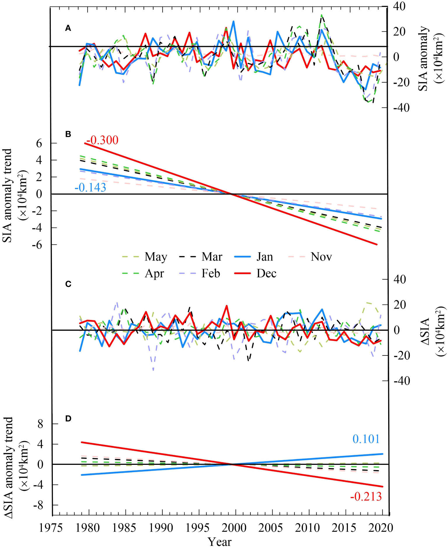
Figure 1 (A) Monthly SIA anomaly from 1979 to 2020. The corresponding colors are shown in the legend; (B) individual SIA anomaly trends corresponding to (A); (C) SIA increments/decrements relative to the SIA in the previous month (ΔSIA); and (D) individual ΔSIA anomaly trend. Due to the small amount of sea ice present off the coast of the Bering Sea from July to October, the trends are ignored during this period. The December and January data are labeled by solid lines, while the data representing other months are labeled with dashed lines.

The mean value and standard deviation distributions of ΔSIC_1-12 are summarized in Figure 2. In Figure 2A, the maximum mean ΔSIC_1-12 value is found in Anadyr Gulf, reaching 45.5%. Values above 30% are found covering the portion of the sea around St. Lawrence Island, the Gulf of Anadyr, and Nunivak Island, where the standard deviations (shown in Figure 2B) are also larger than 20%. Large sea ice variabilities (i.e., corresponding to regions with high standard deviation values) are not confined to sea ice edges but are also observed in the northeast portion of the Bering Sea, suggesting a slight difference from the findings of Liu et al. (2007) derived based on an SIC dataset from 1979 to 2002. In their study, the standard deviation in Anadyr Gulf is less than that obtained in the present study. The annual ΔSIA_1-12 in January (Figure 3) is computed as the integrated ΔSIC_1-12 multiplied by the area on the grid-cell level, except for points with SIC values less than 5% in January. The maximum January ΔSIA_1-12 anomaly is found in 2012, with a value of 16.4×10⁴ km². Although the Bering Sea has the smallest SIA in January 2018 (Stabeno and Bell, 2019), the minimum ΔSIA_1-12 anomaly is observed in 1979, with a value of -16.5×10⁴ km².

FIGURE 2

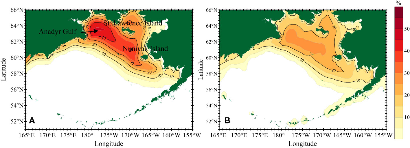
Figure 2 (A) Mean SIC increment in January in contrast to the last month from 1979 to 2017; (B) standard deviation of the SIC increment in January.

FIGURE 3

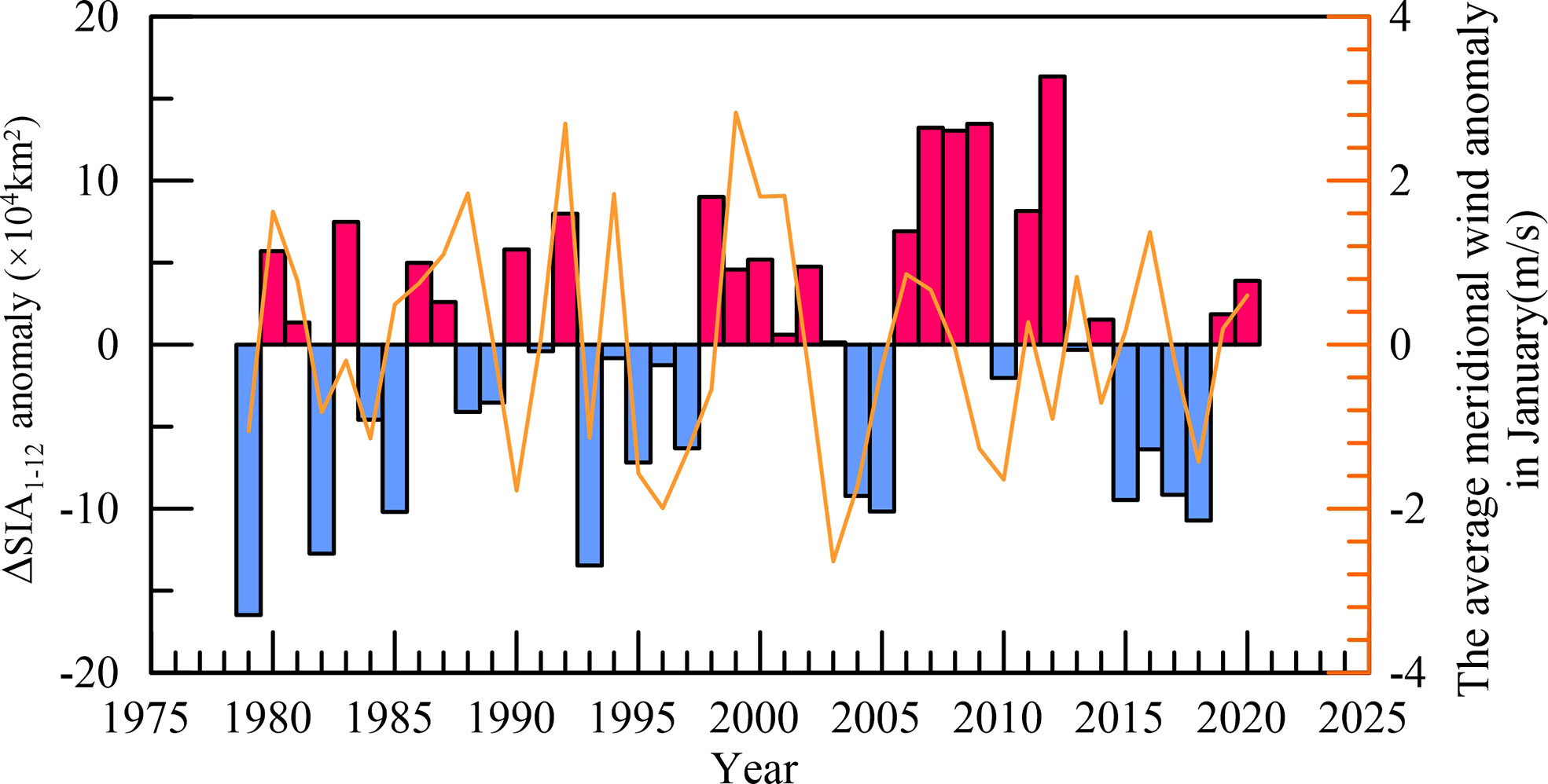
Figure 3 January ΔSIA_1-12 anomalies. The brown solid line denotes the average v-component wind in January in the regions in which the ΔSIC_1-12 values shown in Figure 2A are larger than 5%.

Considering the direct driving effects of wind on sea ice from 1979-2020, the mean January meridional wind values are acquired in the region where the ΔSIC_1-12 values shown in Figure 2A are greater than 5%, as indicated by the brown solid line in Figure 3. All V-component wind values are negative (not shown), suggesting that northerly winds prevail over the Bering Sea in boreal winter. However, the magnitude of the north wind is not consistent with the ΔSIA anomaly. For example, in 2004, the maximum northerly wind indicated in the historic record does not cause a significant ΔSIA increase in January. Similarly, in 2000, the minimum northerly wind in the historical record does not cause an abnormal SIA decrease. The correlation coefficient between them is found to be as low as 0.258, indicating that the SIA increases driven by northerly winds are weak in early winter.

In addition, ΔSIA_1-12 seems to exhibit two high-frequency behaviors, although the relatively short period of record (42 years) limits our ability to analyze these behaviors. Wyllie-Echeverria and Wooster (1998) show that at least two environmental variability scales exist on the Bering Sea shelf: interannual fluctuations between warm and cool years and multiple years of warm or cool states. As shown in Figure 3, before 1992, the ΔSIA_1-12 record features clear 1-2-year fluctuations. After 1992, the ΔSIA_1-12 values appear to exhibit 3-5-year fluctuations, suggesting that another process may exert a strong influence on the sea ice. Given that there is significant sea ice variability, it is instructive to quantify the sea ice variability in the Bering Sea using the empirical orthogonal function (EOF) approach rather than generating one variability index for sea ice using ΔSIA_1-12.

3.2 EOF modes

To assess the existence of two processes, one causing 1-2-year fluctuations and the other leading to 3-5-year fluctuations in terms of sea ice variability, the EOF analysis method is used to decompose ΔSIC_1-12 for the period from 1979-2020 and compute the patterns of ΔSIC_1-12 in both space and time. The explained variances of the first two EOFs (35.20% for EOF1 and 25.38% for EOF2) are much larger than those of the other EOFs (i.e., 11.54% for EOF3). The autocorrelations of EOF1, EOF2, and EOF3 are computed as follows:

$${\text{R}}_{\text{EOF}1}\left(0\right)=1,{\text{ R}}_{\text{EOF}1}\left(1\right)=0.0615,{\text{ R}}_{\text{EOF}1}\left(2\right)=0.0031,{\text{ R}}_{\text{EOF}1}\left(3\right)=0.0827,\dots$$

$${\text{R}}_{\text{EOF}2}\left(0\right)=1,{\text{R}}_{\text{EOF}2}\left(1\right)=-0.0018,{\text{ R}}_{\text{EOF}2}\left(2\right)=-0.0490,{\text{R}}_{\text{EOF}2}\left(3\right)=-0.0157,\dots$$

$${\text{R}}_{\text{EOF}3}\left(0\right)=1,{\text{R}}_{\text{EOF}3}\left(1\right)=-0.0025,{\text{R}}_{\text{EOF}3}\left(2\right)=0.0008,{\text{R}}_{\text{EOF}3}\left(3\right)=0.0002,\dots$$

Based on these coefficients and the method proposed by North et al. (1982), it is certain that EOF1 and EOF2 are statistically significant and distinct from each other. The EOF1 mode (shown in Figure 4A) features negative ΔSIC anomalies south of St. Lawrence Island, corresponding to the area with high mean ΔSIC_1-12 values (seen in Figure 2A). EOF2 (shown in Figure 4B) shows positive ΔSIC anomalies around St. Lawrence Island. The standardized PCs corresponding to EOF1 (PC1) and EOF2 (PC2) are shown in Figures 4C, D respectively. PC1 shows low-frequency oscillations of 3-5 years. PC2 exhibits high-frequency oscillations of 1-2 years. The moving correlation coefficients of ΔSIA_1-12 with PC1 (Figure 4E) and PC2 (Figure 4F) respectively are computed.

FIGURE 4

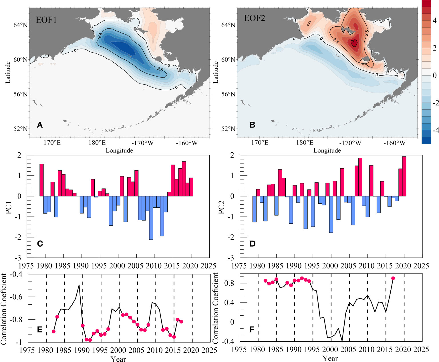
Figure 4 Spatial patterns of the first two dominant EOF modes representing the early winter SIC increment in January relative to that in December: (A) EOF1 and (B) EOF2. Panels (C) and (D) reflect the standardized PCs corresponding to the two dominant EOF modes (PC1 and PC2, respectively). Panels (E) and (F) provide the correlation coefficients of the SIA increment with PC1 and PC2, respectively, derived based on the moving correlation method with a 7-year window. Here, the pink circles denote the criterion of the significance level exceeding 95%.

In PC1, most of correlation coefficients exceed 70% from 1991-2017. Most of the correlation coefficients reach the significance level criterion exceeding 95% as well. In PC2, only from 1981 to 1994 do the derived correlation coefficients meet the significance level criterion exceeding 95%. In other words, prior to 1991, the high-frequency oscillation in PC2 corresponds to ΔSIA_1-12. After 1991, the 3 to 5-years oscillation of PC1 is basically the same as that of ΔSIA_1-12. The first two EOF patterns totally explain approximately 60% of the variance, and can reflect the basic spatiotemporal variations of ΔSIA_1-12.

In addition, there are several years with a weak negative correlation between PC1 and ΔSIA_1-12, such as 1989, 1998 and 2005. Two minor regime shifts are observed on the decadal time scale in the Pacific Decadal Oscillation (PDO) multidecadal climate regime. The first shift occurs in 1989, and the second shift occurs in 1998 (Overland and Stabeno, 2004). In the context of climate change, the spatiotemporal variations in sea ice are modulated by a relatively large-scale climate system [e.g. PDO, Zhang et al. (2010)], while solitary regime shift events are not reflected in the PC1 mode. When analyzing the correlation between the Arctic Oscillation index and the gridded SLPs north of 20°N, Zhao et al. (2006) observed comparable uncorrelated years as well, which are closely related to the shift of Arctic climate system. As a result, the interpretation of PC1 in the paper cannot be generalized to these solitary regime shift events.

3.3 Composite analysis of SSTs and sea surface velocities in early winter

In EOF1, the region with the most significant sea ice changes is in the outermost area close to the open water (in Figure 4A). Because the influence of the meridional wind is weak, ocean heat should be considered when analyzing this region. Sea ice can be transported southward by the very strong northeasterly winds to areas with relatively warm SSTs in early winter. Meanwhile, the southern warm seawater can also inhibit the southward advance of sea ice. Stabeno et al. (2007) suggested that relatively warm summertime ocean temperatures delay the southward advection of sea ice during winter. In fact, the properties of warm water in summer change significantly following evaporation, heat conduction, and heat transport processes. Generally, the decisive factor inhibiting sea ice advances in early winter is the residual heat in the seawater in November or December. The positive- and negative-phase years identified in PC1 are selected and used to facilitate the composite difference (positive years minus negative years) analysis on the SST and sea surface velocity in November and December.

In the SST composite map (Figure 5), both November and December, before sea ice freezes, are characterized by warm water to the south of St. Lawrence Island and to the west and south of Nunivak Island. In the sea surface velocity composite map, it is evident that a strong meridional current anomaly on the order of 0.15 m/s or more covers the Bering Sea shelf in December, consistent with the areas where the sea ice changed significantly in EOF1. In contrast, no significant meridional current anomaly is found in November. The abnormally warm SST and northward current indicates that the above-normal sea surface poleward heat transport that occurs south of St. Lawrence Island in early winter is probably to be an import modulator of the wintertime SIC.

FIGURE 5

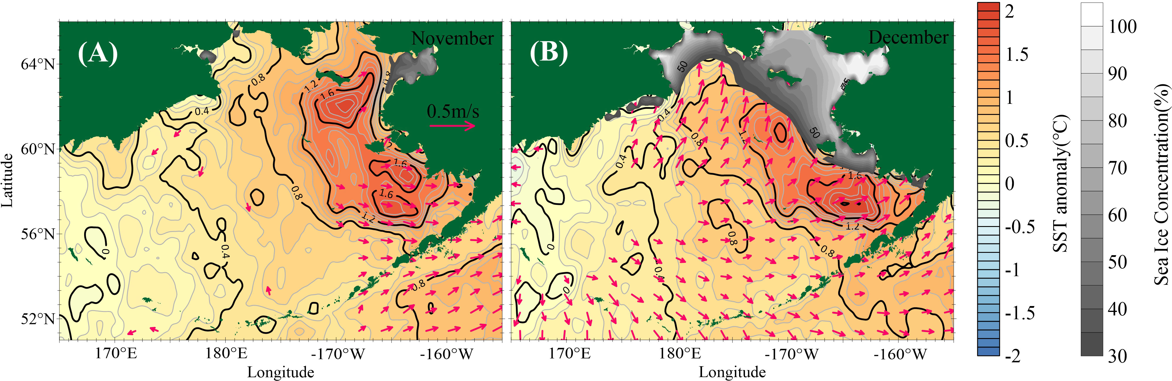
Figure 5 Composite difference map of the mean SST anomaly and sea surface velocity anomaly derived from the PC1 index in November (A) and December (B) from 1993 to 2020. The velocity is shown when the value is higher than 0.1 m/s. The corresponding 42-year mean SIC is represented by black-and-white shading.

In the Barents and Kara Seas, more inflowing ocean heat can result in the formation of less sea ice during the cold season, thus leading to a high anticorrelation between water heat transport from the Atlantic Ocean and the cold season SIA, with a value of r=-0.76 (Shu et al., 2021). In this work, we could not obtain the poleward heat transport of the Alaska slope current due to the relative scarcity of data. Instead, the correlation between the poleward heat transport on each grid cell and PC1 is calculated in the mixed layer without considering the influence of topography on the Ekman transport and heat transport across the mixed layer. An extensive area comprising significant positive correlations in December (in Figure 6B) is observed near the sea ice edge, covering the region south of St. Lawrence Island and north of the 100-m isobaths, corresponding to the region indicated to have significant spatial changes by EOF1. A weak positive correlation is observed in November (Figure 6A) near St. Lawrence Island, although the composite SST maps exhibit agreement between November and December.

FIGURE 6

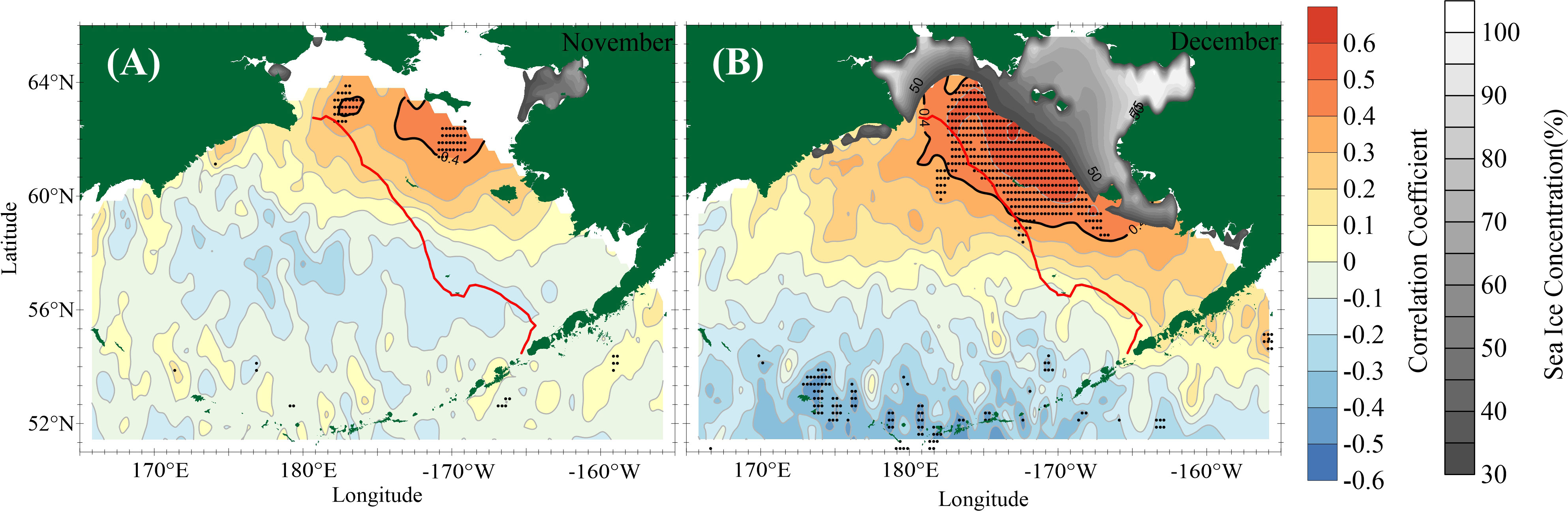
Figure 6 Correlation coefficients between PC1 and poleward heat transport in November (A) and December (B). The black dots indicate locations where the criterion of a significance level exceeding 95% is met. The red dashed line indicates the 100-m isobath.

The preceding explanation essentially highlights the fact that, in the positive phase of EOF1, warm water expands in the Bering Sea shelf during November and December. Because of the abnormal northward surface current in December, there is a large-scale northward oceanic heat transport south of St. Lawrence Island, preventing sea ice from expanding southward. The northward oceanic heat transport covers the entire middle continental shelf in the Bering Sea. There is no substantial correlation between SST and PC1 in the Bering Sea shelf area in either November or December (not shown), indicating that warm water in November and December is the premise to inhibit the southward expansion of sea ice, and its decisive role is the abnormal northward warm current.

3.4 The influence of warm advection on SST

Generally, a positive heat budget occurs from April to September in the Bering Sea, causing SSTs to increase. From October to March, the negative oceanic heat budget modulates SST decreases. Especially in winter, large air-sea temperature differences lead to rapidly declining SSTs. The ocean energy budget plays an essential role in determining sea-ice growth and melt rates, especially near the ice edge where ice can be advected into waters substantially above freezing (Bitz et al., 2005). It is thus necessary to explore the contributions of different heat budget terms to sea ice changes.

SSTs are generally controlled by the net air-sea heat flux. The substantially air-sea heat flux causes a rapid reduction in SST from November to December as a result of the heat release from the ocean to the atmosphere. The advection delivers a large amount heat from low latitudes in Bering Sea shelf, preventing the SST from further decreasing. The estimates derived herein show that the contribution of the air-sea heat flux to the SST is 10~100 times larger than the contribution of the warm advection in December. However, the computed correlation of the December net air-sea heat flux with PC1 is weak from 1983 to 2009 (not shown), which implies that the massive air-sea heat flux is not the primary driver of the EOF1 spatial pattern.

Here, diagnostic ECCO2 V4r2 results are applied to estimate the explained variance (EV) of the air-sea net heat flux, advection, and diffusion on the potential temperature variance from 1992 to 2011. The conservation equation can be written as follows:

$\begin{array}{ll}\underset{T_{tend}}{\underbrace{\frac{\partial \theta }{\partial t}}}=\underset{T_{ad}}{\underbrace{-\nabla ·\left({\overrightarrow{u}}_{res}\theta \right)}}+\underset{T_{di}}{\underbrace{D_{\theta }}}+\underset{T_{forc}}{\underbrace{F_{\theta }}}& \text{(6)}\end{array}$

where T_tend represents the potential temperature (θ) tendency, T_ad is the potential temperature tendency due to seawater advection, ${\overrightarrow{u}}_{res}\equiv \left(U_{res},{\text{ V}}_{\text{res}}, W_{res}\right)$ are the zonal, meridional, and vertical components of the residual mean velocity, respectively, T_forc represents the potential temperature tendency due to the net (turbulent and radiative) surface heat flux, and T_di is the potential temperature tendency due to parameterized (iso-neutral and dia-neutral) mixing. Considering the significant area in PC1, the data in the area indicated by the red quadrilateral in Figure 7A are chosen (and integrated throughout the whole water column). The EVs of T_forc, T_di, and T_ad on T_tend are then calculated according to the following formulas:

$\begin{array}{ll}Var\left(T_{tend}\right)=Var\left(T_{ad}\right)+Var\left(T_{di}\right)+Var\left(T_{forc}\right)+2Cov\left(T_{ad}, T_{di}\right)+2Cov\left(T_{ad},T_{forc}\right)+2Cov\left(T_{di},T_{forc}\right)& \text{(7)}\end{array}$

$$EV\left(T_{ad}\right)=\frac{Var\left(T_{ad}\right)}{Var\left(T_{tend}\right)}$$

$$EV\left(T_{di}\right)=\frac{Var\left(T_{di}\right)}{Var\left(T_{tend}\right)}$$

$$EV\left(T_{forc}\right)=\frac{Var\left(T_{forc}\right)}{Var\left(T_{tend}\right)}$$

$$EV\left(Cov\right)=\frac{Var\left(Cov\right)}{Var\left(T_{tend}\right)}$$

FIGURE 7

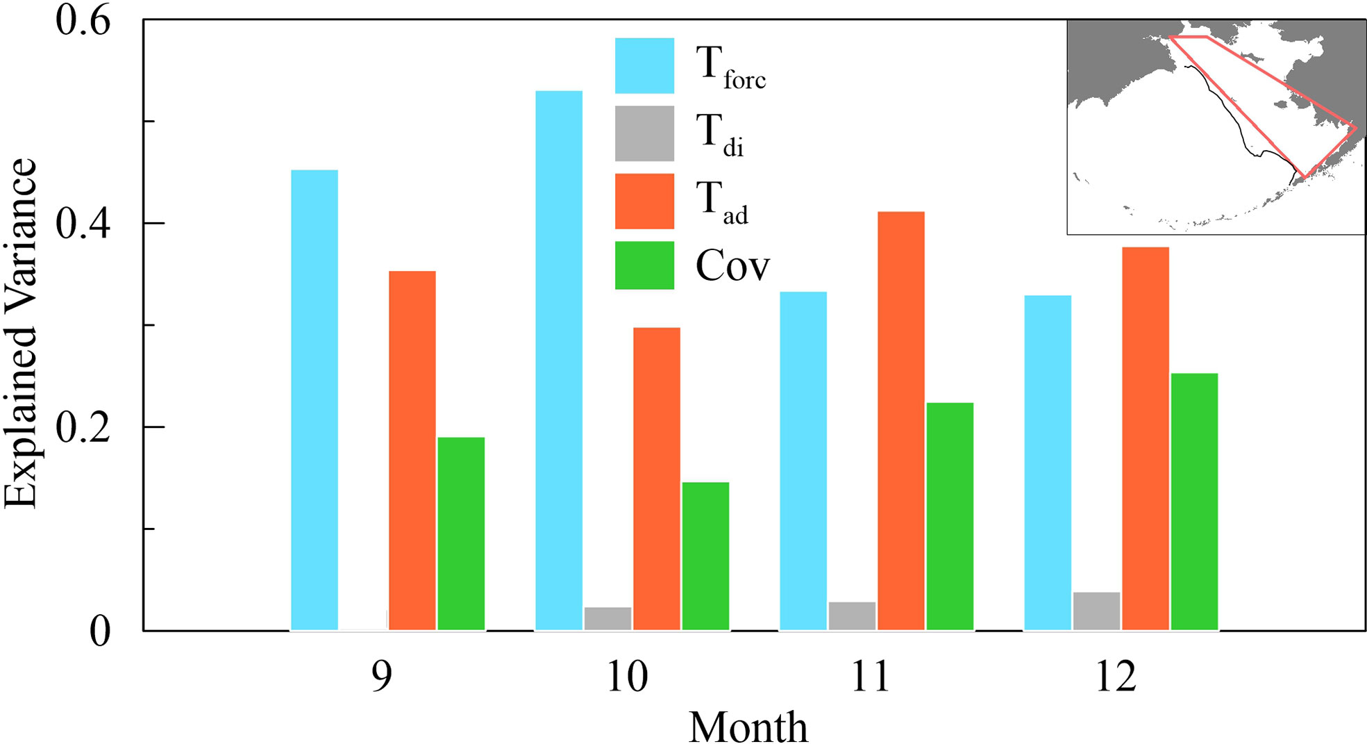
Figure 7 Separate EVs of T_ad, T_di, and T_forc, and the total covariance between these terms and T_tend in September, October November, and December. The temporal range spans from 1992 to 2011. The calculation region north of the 100-m isobath is denoted by the dashed line.

Where Var(Cov)=2Cov(T_ad, T_di)+2Cov(T_ad,T_forc)+2Cov(T_di,T_forc) . Var denotes the variance corresponding to the specific terms and Cov denotes the covariances between each term. The corresponding EVs are shown in Figure 7.

The EVs of T_forc in September and October are larger than those of T_ad (in Figure 7); thus, large air-sea heat fluxes mainly determine the local SST trends. From November to December, the T_forc EV clearly decreases, from 53.1% in October to 33.4% in November. The T_ad EV increases from 29.8% to 41.2% over this period, indicating that the advection process plays a major role in the SST trend. In the EVs of the total covariances, the covariance of T_ad and T_forc also plays a leading role (not shown). These results show that in early winter, the strong advection process critically impacts the SST, even exceeding the influence of air-sea heat fluxes. Here, we used the observed and remotely sensed datasets described above to calculate the correlation coefficient between the advection term ($-\overrightarrow{V}·\nabla T$) and PC1. The derived significant positive correlations cover the Bering Sea shelf with coefficients reaching 68% near the sea ice edge (above the 95% confidence level) in November and December (Figure 8).

FIGURE 8

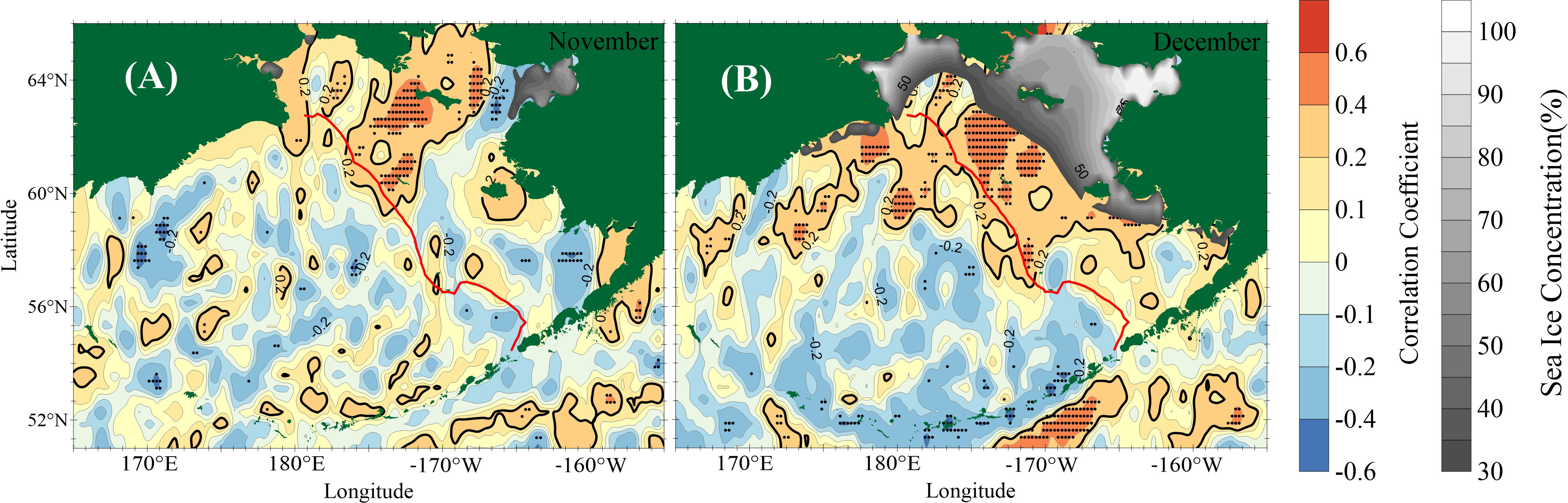
Figure 8 Correlation coefficients between PC1 and the advection term ($-\overrightarrow{V}·\nabla T$) in November (A) and December (B). The black dot denotes locations at which the criterion of a significance level exceeding 95% is met. The red dashed line indicates the 100-m isobath.

This shows that the dominant factor regulating the interannual variability of SST in the Bering Sea shelf shifts from air-sea net heat flux to warm advection in early winter, indicating that strong local warm advection prevents further cooling of the sea surface due to net air-sea heat flux in early winter, and explaining the close correlation of PC1 with the northward oceanic heat transport in the Bering Sea shelf and the weak correlation with air-sea net heat flux (Figure 6A). The study concludes that the explanation of high summertime SST leading to small SIAs in the later stage of the year may be one-sided. On the one hand, SSTs in December do not show a significant correlation with PC; on the other hand, air-sea interaction is still the dominant regulating SST in December, but its correlation with PC1 is modest.

3.5 The effect of wind on sea ice

SSTs in the positive phase of EOF1 are abnormally warm in November and December (Figure 5). However, the northward oceanic heat transport exhibits a clear positive relationship with PC1 only in December. To investigate the impact of meridional current on northward oceanic heat transport, we decompose vT in equation (1) as follows: $vT=\left(\overline{v}+v\text{'}\right)\left(\overline{T}+T\text{'}\right)=\overline{v}\overline{T}+\overline{v}T\text{'}+v\text{'}\overline{T}+v\text{'}T\text{'}$ (8)

where the superscript represents the anomaly value. Figure 9 shows the interannual variations of the last three decomposition terms.

FIGURE 9

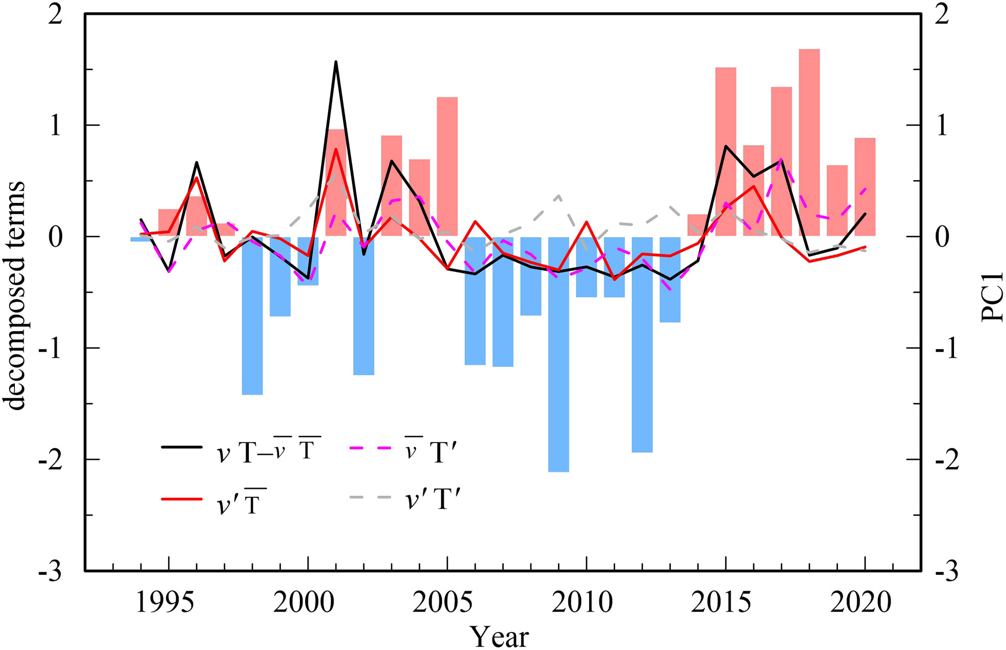
Figure 9 Multiyear variations in $vT-\overline{v}\overline{T}$, $\overline{v}T\text{'}$, $v\text{'}\overline{T}$ and v'T' from 1993-2020 averaged in the region where the confidence levels exceeded 95% (as shown in Figure 6B). The bar denotes the PC1 index. The time series of the decomposition terms are added for one year to better visualize the consistency among the terms.

When comparing the interannual variation in $vT-\overline{v}\overline{T}$, none of the three decomposition terms is completely dominant. In other words, the meridional current is as important as SST in the poleward heat transport anomaly. The meridional current and SST together modulate the interannual variation of ΔSIA observed in early winter.

The northward oceanic heat transport in the mixed layer may be further decomposed into Ekman-driven poleward oceanic heat transport and geostrophic oceanic heat transport. The calculation shows that the mean Ekman-driven poleward heat transport in December is 36 times that of the geostrophic current in the Bering Sea shelf. Ekman-driven poleward oceanic heat transport has a dominant role in the overall oceanic heat transport. The significant rise in sea surface temperature induced by Ekman transport reaches more than 0.2°C/d in the region with considerable EOF1 reduction in December (Figure 10). The abnormal northeast wind does not currently play a dynamic role in pushing southward movement of sea ice, but it does generate a strong Ekman transport in the south open water, resulting in an increase in northward oceanic heat transport.

FIGURE 10

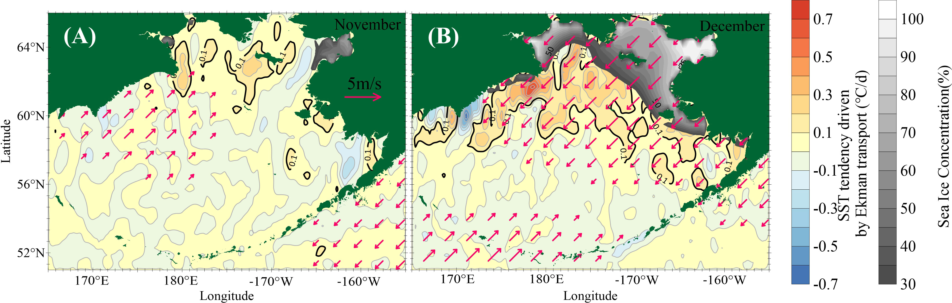
Figure 10 Composite difference maps of the mean wind anomaly and $-\overrightarrow{V_{ek}}·\nabla T$ anomaly derived using the PC1 index in November (A) and December (B) from 1993 to 2020. The velocity is shown when its value is faster than 1 m/s.

4 Discussion

Unlike most prior researches that have concentrated on the inter-seasonal variation of SIA in the Bering Sea (e. g. Singarayer and Bamber, 2003; Sasaki and Minobe, 2005; Liu et al., 2007; Liang et al., 2020), this study focuses on the intra-seasonal changes in sea ice. However, the spatial patterns derived from SIA increment in January is largely comparable with the inter-seasonal patterns of average SIC derived by Liang et al. (2020) for entire Arctic winter (December-March). The EOF1 described in this paper is also similar with the spatial pattern derived by Liu et al. (2007), who presented a dipole spatial pattern between the sea of Okhotsk and the Bering Sea during the winter season. The consistency of spatial patterns between the inter-seasonal and intra-seasonal change in sea ice underscores the importance of SIA increment in January to the sea ice change throughout the winter.

Wind drag plays a very important role in the sea ice change in the Bering Sea (Sasaki and Minobe, 2005). Abnormal SIA is frequently associated with early atypical wind field (Niebauer et al., 1999). Sasaki and Minobe (2005) investigated the interannual variability of sea ice in the Bering Sea and its relation to atmosphere fluctuations, and even suggested that a better understanding of the wind anomalies over the Bering Sea are important to know the interannual sea ice variability in the Bering Sea. However, on an intra-seasonal scale, the increment of SIA in January is not related to wind field anomaly. It is proposed in this paper that the southward advance of sea ice driven by the wind is constrained in early winter, and this constraint is produced by warm advection in the preceding month. This study clearly demonstrates that the effect of the wind on sea ice varies across time scales, from advancing sea ice southward on an inter-seasonal scale to driving heat transport toward ice region on an intra-seasonal scale due to the action of generating Ekman transport.

Prior to 1994, there exists a substantial correlation between PC2 and ΔSIA in January. Preliminary research suggests that EOF2 may be associated to local sea-air heat flux. Further research on PC2 can explain sea ice change at the end of the last century, and clarify the cause for the shift in the mechanism of sea ice change by comparing the recent sea ice change. In addition, future research is also needed to evaluate the time evolution of the northward heat transport from the intra-seasonal cycle, including the impacts of anomalous winds, surface energy fluxes, fluctuating current and mesoscale eddy effects.

5 Summary

From 1979 to 2020, the SIA of the Bering Sea shows a declining tendency in all months. The highest negative trend appears in December with a value of -2000 km²/a. We also estimate the increment or decrement of SIAs (ΔSIA) in all months. In contrast to the SIA tendency observed in the Bering Sea, the observational ΔSIA derived herein exhibits a considerable positive trend on the order of 1010 km²/a in January. EOF analysis method is employed to decompose the spatiotemporal variation in January ΔSIA. The first two spatial modes (EOF1 and EOF2) can explain more than 60% of the variance. EOF1 features negative ΔSIC anomalies south of St. Lawrence Island, consistent with the spatial distribution of the multiyear mean and standard deviation. EOF2 shows positive ΔSIC anomalies around St. Lawrence Island.

We examine what drives the specific spatial patterns of EOF1 by applying composite and correlation analytical approaches. The positive EOF1 pattern is dominated by comparatively warm SSTs and strong meridional currents over the Bering Sea shelf in December. The broad strong poleward oceanic heat transport in December produces ocean heat flux convergence toward the ice edge and explains the temporal variation in EOF1. Different from the prior understanding, January ΔSIA is not the result of abnormal northeast winds, but is modulated by northward poleward oceanic heat transport.

The effect of ocean heat transport on sea ice is discussed explicitly in the paper. During sea ice advancing southward, on the one hand, although the SST tendency in December is governed by the net air-sea heat flux over the Bering Sea shelf, its interannual variation is mostly dependent on warm advection. The local ocean heat storage driven by advection near the ice edge results in the inhibition of the southward expansion of sea ice in the later period. On the other hand, the northeast wind anomaly in December no longer plays the role of a dynamic process advancing southward movement of sea ice and instead drives northward ocean heat transport in the ice edge, further delaying sea ice advance. In the early winter, ocean heat transport dominates and regulates the Bering Sea SIA in competition with atmospheric forcing.

Although the January climatological mean value of ΔSIA only accounts for 36% of the maximum SIA, the PC1 derived from it has a close inverse correlation with the maximum SIA, with a correlation coefficient of -0.76. PC1 can be utilized as the prediction index for the Bering Sea maximum SIA. As for whether it can predict the local ecosystem changes, it is worth further study.

Data availability statement

The original contributions presented in the study are included in the article/supplementary material. Further inquiries can be directed to the corresponding author.

Author contributions

WW and JS contributed to the development, planning, data collection, data analysis and interpretation; CJ and XG provided financial support and gave some important suggestions. All authors contributed to the writing of the manuscript.

Acknowledgments

Thank two anonymous reviewers for their meticulous review. The paper is funded by the Scientific Research Foundation of the Third Institute of Oceanography, MNR, China (No. 2016023), the Global Change and Air-sea Interaction II (GASI-01-NPAC-STsum), the National Natural Science Foundation of China (42130406), the National Key Research and Development Program of China (2018YFA0605901) and the National Natural Science Foundation of China (General Program) (42076228).

Conflict of interest

The authors declare that the research was conducted in the absence of any commercial or financial relationships that could be construed as a potential conflict of interest.

Publisher’s note

All claims expressed in this article are solely those of the authors and do not necessarily represent those of their affiliated organizations, or those of the publisher, the editors and the reviewers. Any product that may be evaluated in this article, or claim that may be made by its manufacturer, is not guaranteed or endorsed by the publisher.

References

Alabia I. D., Molinos J. G., Saitoh S. I., Hirata T., Hirawake T., Mueter F. J. (2020). Multiple facets of marine biodiversity in the pacific Arctic under future climate. Sci. Total Environ. 744, 140913. doi: 10.1016/j.scitotenv.2020.140913

PubMed Abstract | CrossRef Full Text | Google Scholar

Alexander V., Niebauer H. J. (1981). Oceanography of the eastern Bering Sea ice-edge zone in spring. Limnol. Oceanogr. 26 (6), 1111–1125. doi: 10.4319/lo.1981.26.6.1111

CrossRef Full Text | Google Scholar

Babb D. G., Galley R. J., Asplin M. G., Lukovich J. V., Barber D. G. (2013). Multiyear sea ice export through the Bering strait during winter 2011-2012. J. Geophys. Res.: Oceans 118 (10), 5489–5503. doi: 10.1002/jgrc.20383

CrossRef Full Text | Google Scholar

Bitz C. M., Holland M. M., Hunke E. C., Moritz R. E. (2005). Maintenance of the sea-ice edge. J. Clim. 18, 2903–2921. doi: 10.1175/JCLI3428.1

CrossRef Full Text | Google Scholar

Brown Z. W., Arrigo K. R. (2012). Contrasting trends in sea ice and primary production in the bering sea and arctic ocean. ICES J. Mar. Sci. 69 (7), 1180–1193. doi: 10.1093/icesjms/fst048

CrossRef Full Text | Google Scholar

Cavalieri D. J., Parkinson C. L. (2012). Arctic Sea ice variability and trends 1979-2010. Cryosphere 6 (4), 881–889. doi: 10.5194/tc-6-881-2012

CrossRef Full Text | Google Scholar

Comiso J. (2015). Bootstrap Sea ice concentrations from nimbus-7 SMMR and DMSP SSM/I-SSMIS, version 2 (Boulder, CO, USA: NASA DAAC at the National Snow and Ice Data Center).

Google Scholar

Comiso J. C., Meier W. N., Gersten R. (2017). Variability and trends in the Arctic Sea ice cover: Results from different techniques. J. Geophys. Res.: Oceans 122 (8), 6883–6900. doi: 10.1002/2017JC012768

CrossRef Full Text | Google Scholar

de la Vega C., Jeffreys R. M., Tuerena R., Ganeshram R., Mahaffey C. (2019). Temporal and spatial trends in marine carbon isotopes in the Arctic ocean and implications for food web studies. Global Change Biol. 25 (12), 4116–4130. doi: 10.1111/gcb.14832

CrossRef Full Text | Google Scholar

Hunt G. L. Jr., Coyle K. O., Eisner L. B., Farley E. V., Heintz R. A., Mueter F., et al. (2011). Climate impacts on eastern Bering Sea foodwebs: A synthesis of new data and an assessment of the oscillating control hypothesis. ICES J. Mar. Sci. 68 (6), 1230–1243. doi: 10.1093/icesjms/fsr036

CrossRef Full Text | Google Scholar

Hunt G. L., Yasumiishi E. M., Eisner L. B., Stabeno P. J., Decker M. B. (2020). Climate warming and the loss of sea ice: The impact of sea-ice variability on the southeastern Bering Sea pelagic ecosystem. ICES J. Mar. Sci. 79 (3), 937–953. doi: 10.1093/icesjms/fsaa206

CrossRef Full Text | Google Scholar

Kalnay E., Kanamitsu M., Kistler R., Collins W., Deaven D., Gandin L., et al. (1996). The NCEP/NCAR 40-year reanalysis project. Bull. Am. Meteorol. Soc. 77 (3), 437–472. doi: 10.1175/1520-0477(1996)077<0437:TNYRP>2.0.CO;2

CrossRef Full Text | Google Scholar

Kearney K. A., Alexander M., Aydin K., Cheng W., Hermann A. J., Hervieux G., et al. (2021). Seasonal predictability of Sea ice and bottom temperature across the Eastern Bering Sea shelf. J. Geophys. Res.: Oceans 126 (11), 1–21. doi: 10.1029/2021JC017545

CrossRef Full Text | Google Scholar

Liang Y., Bi H., Wang Y., Zhang Z., Huang H. (2020). Role of atmospheric factors in forcing Arctic sea ice variability. Acta Oceanol. Sin. 39 (9), 60–72. doi: 10.1007/s13131-020-1629-6

CrossRef Full Text | Google Scholar

Li L., Miller A. J., McClean J. L., Eisenman I., Hendershott M. C. (2014). Processes driving sea ice variability in the Bering Sea in an eddying ocean/sea ice model: Anomalies from the mean seasonal cycle. Ocean Dynamics 64 (12), 1693–1717. doi: 10.1007/s10236-014-0769-7

CrossRef Full Text | Google Scholar

Liu J., Zhang Z., Horton R. M., Wang C., Ren X. (2007). Variability of north pacific sea ice and East Asia-north pacific winter climate. J. Climate 20 (10), 1991–2001. doi: 10.1175/JCLI4105.1

CrossRef Full Text | Google Scholar

Meneghello G., Marshall J., Timmermans M. L., Scott J. (2018). Observations of seasonal upwelling and downwelling in the Beaufort Sea mediated by sea ice. J. Phys. Oceanogr. 48 (4), 795–805. doi: 10.1175/JPO-D-17-0188.1

CrossRef Full Text | Google Scholar

Menemenlis D., Campin J. M., Heimbach P., Hill C., Lee T., Nguyen A. T., et al. (2008). ECCO2: High resolution global ocean and sea ice data synthesis. Mercator Ocean Quarterly Newsletter. 31(October), 13–21.

Google Scholar

Mueter F. J., Litzow M. A. (2008). Sea Ice retreat alters the biogeography of the Bering Sea continental shelf. Ecol. Appl. 18 (2), 309–320. doi: 10.1890/07-0564.1

PubMed Abstract | CrossRef Full Text | Google Scholar

Nakanowatari T., Inoue J., Sato K., Kikuchi T. (2015). Summertime atmosphere-ocean preconditionings for the Bering Sea ice retreat and the following severe winters in north America. Environ. Res. Lett. 10 (9), 094023. doi: 10.1088/1748-9326/10/9/094023

CrossRef Full Text | Google Scholar

Niebauer H. J. (1988). Effects of El nino-southern oscillation and north pacific weather patterns on interannual variability in the subarctic Bering Sea. J. Geophys. Res. 93 (C5), 5051–5068. doi: 10.1029/JC093iC05p05051

CrossRef Full Text | Google Scholar

Niebauer H. J. (1998). Variability in Bering Sea ice cover as affected by a regime shift in the north pacific in the period 1947-1996. J. Geophys. Res.: Oceans 103 (C12), 27717–27737. doi: 10.1029/98JC02499

CrossRef Full Text | Google Scholar

Niebauer H. J., Bond N. A., Yakunin L. P., Plotnikov V. V. (1999). “An update on the climatology and Sea ice of the Bering Sea,” in Dynamics of the Bering Sea, (Fairbanks, Alaska, USA), 1–28. doi: 10.4027/dbs.1999

CrossRef Full Text | Google Scholar

North G. R., Bell T. L., Cahalan R. F., Moeng F. J. (1982). Sampling errors in the estimation of empirical orthogonal functions. Monthly Weather Rev. 110 (7), 699–706. doi: 10.1175/1520-0493(1982)110<0699:SEITEO>2.0.CO;2

CrossRef Full Text | Google Scholar

Ohshima K. I., Tamaru N., Kashiwase H., Nihashi S., Nakata K., Iwamoto K. (2020). Estimation of Sea ice production in the Bering Sea from AMSR-e and AMSR2 data, with special emphasis on the anadyr polynya. J. Geophys. Res.: Oceans 125 (7), e2019JC016023. doi: 10.1029/2019JC016023

CrossRef Full Text | Google Scholar

Overland J. E., Stabeno P. J. (2004). Is the climate of the Bering Sea warming and affecting the ecosystem? Eos Trans. Am. Geophys. Union 85 (33), 309. doi: 10.1029/2004EO330001

CrossRef Full Text | Google Scholar

Parkinson C. L., Cavalieri D. J., Gloersen P., Zwally H. J., Comiso J. C. (1999). Arctic sea ice extends, areas, and trend, 1978–1996. Journal of Geophysical Research C: Oceans 104, 20837–20856. doi: 10.1029/1999JC900082

CrossRef Full Text | Google Scholar

Parkinson C. L., Cavalieri D. J. (2008). Arctic Sea ice variability and trends 1979–2006. J. Geophys. Res. 113, C07003. doi: 10.1029/2007JC004558

CrossRef Full Text | Google Scholar

Parkinson C. L., DiGirolamo N. E. (2021). Sea Ice extents continue to set new records: Arctic, Antarctic, and global results. Remote Sens. Environ. 267 (September), 112753. doi: 10.1016/j.rse.2021.112753

CrossRef Full Text | Google Scholar

Pease C. H. (1980). Eastern Bering Sea Ice processes. Monthly Weather Rev. 108 (12), 2015–2023. doi: 10.1175/1520-0493(1980)108<2015:ebsip>2.0.co;2

CrossRef Full Text | Google Scholar

Rayner N. A., Parker D. E., Horton E. B., Folland C. K., Alexander L., Rowell D. P., et al. (2003). Global analyses of sea surface temperature, sea ice, and night marine air temperature since the late nineteenth century. J. Geophys. Res.: Atmospheres 108 (14), 4407. doi: 10.1029/2002jd002670

CrossRef Full Text | Google Scholar

Sasaki Y. N., Minobe S. (2005). Seasonally dependent interannual variability of sea ice in the Bering Sea and its relation to atmospheric fluctuations. J. Geophys. Res. C: Oceans 110 (5), 1–11. doi: 10.1029/2004JC002486

CrossRef Full Text | Google Scholar

Screen J. A., Simmonds I., Keay K. (2011). Dramatic interannual changes of perennial Arctic sea ice linked to abnormal summer storm activity. J. Geophys. Res. Atmospheres 116 (15), D15105. doi: 10.1029/2011JD015847

CrossRef Full Text | Google Scholar

Shu Q., Wang Q., Song Z., Qiao F. (2021). The poleward enhanced Arctic Ocean cooling machine in a warming climate. Nature Communications 12 (1), 1–10. doi: 10.1038/s41467-021-23321-7

PubMed Abstract | CrossRef Full Text | Google Scholar

Sigler M., Napp J., Stabeno P., Heintz R. A., Lomas M. W., Hunt G. L. Jr. (2016). Variation in annual production of cope- pods, euphausiids, and juvenile walleye pollock in the southeast- ern Bering Sea. Deep Sea Res. II 134, 223–234. doi: 10.1016/j.dsr2.2016.01.003

CrossRef Full Text | Google Scholar

Singarayer J. S., Bamber J. L. (2003). EOF analysis of three records of sea-ice concentration spanning the last 30 years. Geophys. Res. Lett. 30 (5), 1–4. doi: 10.1029/2002gl016640

CrossRef Full Text | Google Scholar

Stabeno P. J., Bell S. W. (2019). Extreme conditions in the Bering Sea, (2017–2018): Record-breaking low Sea-ice extent. Geophys. Res. Lett. 46 (15), 8952–8959. doi: 10.1029/2019GL083816

CrossRef Full Text | Google Scholar

Stabeno P. J., Bond N. A., Salo S. A., Zhao P., Zhang X., Zhou X., et al. (2007). On the recent warming of the southeastern Bering Sea shelf. J. Climate 18 (23–26), 2599–2618. doi: 10.1016/j.dsr2.2007.08.023

CrossRef Full Text | Google Scholar

Stabeno P. J., Farley E. V., Kachel N. B., Moore S., Mordy C. W., Napp J. M., et al. (2012a). A comparison of the physics of the northern and southern shelves of the eastern Bering Sea and some implications for the ecosystem. Deep Sea Res. Part II: Topical Stud. Oceanogr. 65–70, 14–30. doi: 10.1016/j.dsr2.2012.02.019

CrossRef Full Text | Google Scholar

Stabeno P. J., Kachel N. B., Moore S. E., Napp J. M., Sigler M., Yamaguchi A., et al. (2012b). Comparison of warm and cold years on the southeastern Bering Sea shelf and some implications for the ecosystem. Deep Sea Res. Part II: Topical Stud. Oceanogr. 65–70, 31–45. doi: 10.1016/j.dsr2.2012.02.020

CrossRef Full Text | Google Scholar

Wang M., Overland J. E., Stabeno P. (2012). Future climate of the Bering and chukchi seas projected by global climate models. Deep Sea Res. Part II: Topical Stud. Oceanogr. 65–70, 46–57. doi: 10.1016/j.dsr2.2012.02.022

CrossRef Full Text | Google Scholar

Wu R., Chen Z. (2016). An interdecadal increase in the spring Bering Sea ice cover in 2007. Front. Earth Sci. 4 (March). doi: 10.3389/feart.2016.00026

CrossRef Full Text | Google Scholar

Wyllie-Echeverria T., Wooster W. S. (1998). Year-to-year variations in Bering Sea ice cover and some consequences for fish distributions. Fisheries Oceanogr. 7 (2), 159–170. doi: 10.1046/j.1365-2419.1998.00058.x

CrossRef Full Text | Google Scholar

Xiao K., Chen M., Wang Q., Wang X., Zhang W. (2020). Low-frequency sea level variability and impact of recent sea ice decline on the sea level trend in the Arctic ocean from a high-resolution simulation. Ocean Dynamics 70 (6), 787–802. doi: 10.1007/s10236-020-01373-5

CrossRef Full Text | Google Scholar

Yu L., Jin X., Weller R. A. (2008). Multidecade global flux datasets from the objectively analyzed air-sea fluxes (OAFlux) project: Latent and sensible heat fluxes, ocean evaporation, and related surface meteorological variables. oa-2008-01, (January). (Woods Hole, Massachusetts, USA: Woods Hole Oceanographic Institution). doi: 10.1007/s00382-011-1115-0

CrossRef Full Text | Google Scholar

Zhang J. L., Woodgate R., Moritz R. (2010). Sea Ice response to atmospheric and oceanic forcing in the Bering Sea. J. Phys. Oceanogr. 40 (8), 1729–1747. doi: 10.1175/2010jpo4323.1

CrossRef Full Text | Google Scholar

Zhao J., Cao Y., Shi J. (2006). Core region of Arctic oscillation and the main atmospheric events impact on the Arctic. Geophys. Res. Lett. 33 (22), 1–5. doi: 10.1029/2006GL027590

CrossRef Full Text | Google Scholar

Zhou M., Wang H. (2014). Late winter sea ice in the bering sea: Predictor for maize and rice production in northeast China. J. Appl. Meteorol. Climatol. 53 (5), 1183–1192. doi: 10.1175/JAMC-D-13-0242.1

CrossRef Full Text | Google Scholar