Incorporating egg-transporting pathways into conservation plans of spawning areas: An example of small yellow croaker (Larimichthys polyactis) in the East China Sea zone

Backward-in-time Lagrangian model can identify potential spawning areas by reconstructing egg drift trajectories, contributing to accurately designing potential priority conservation plans for spawning areas. In this study, we apply this approach to investigate the small yellow croaker (Larimichthys polyactis) with commercial value in China. A two-step spatial random forest (RF) model is used to predict the occurrence probability and abundance of their eggs and describe the optimal ecological range of environmental factors. A priority protection index (BPPI) of the spawning areas is established by combining the sites with the optimal occurrence and abundance and integrating backward tracking pathways. The result indicates that the model with 1-2 day time lags of environmental variables shows the optimum explanatory power. Temperature and salinity are the most important factors affecting oogenesis and show a regime shift in the response curve. They reflect the physiological regulation of parental sexual maturation by the environment. In addition, egg abundance correlates more strongly with chlorophyll-a (Chl a) concentration and depth, suggesting that parents prefer environments with shallow water and high prey density for spawning activities. The egg retrieval shows that the potential spawning sources are distributed near the southeastern part of the oogenesis site, with a maximum egg dispersal distance of no more than 30 km. This finding confirms that the coastal regions of Jiangsu Province are an important spawning ground for the small yellow croaker, making a significant contribution to the productivity and resilience of the fish.

Introduction

Fish are extremely vulnerable during their early planktonic life stage. Therefore, exploring how the physical-biological interaction mechanism affects that stage is key to revealing fish recruitment (Sundby and Kristiansen, 2015; Casaucao et al., 2021). In the early life stage, most fish would be transported from their spawning grounds to their nursery grounds. The origin and trajectories of eggs and larvae are linked with the source-sink dynamics, which might explain the frequent large-scale recruitment variations (Ospina-Alvarez et al., 2013).

Spawning activities in many marine fish are highly concentrated in space and time, lasting only a few days to a few weeks in the fish spawning aggregation (FSA) areas. These spawning populations usually experienced severe fishing mortality during their spawning migration. Therefore, the spawning population reaching the spawning area represents almost all of the reproductive capacity (Grüss et al., 2014). They are also of great significance to the resilience of fish populations and the sustainability of many fisheries. However, FSA supports highly-productive commercial and subsistence fisheries because their predictability enables fishers to harvest large catches with minimal effort (Sadovy and Domeier, 2005; Erisman et al., 2012). With the intensifying fishing impacts and declining global fishery resources, spawning grounds are also receiving more attention than before (de Mitcheson, 2016; Erisman et al., 2018; Binder et al., 2021).

Globally, fish harvest from spawning aggregations has contributed to rapid regional stock declines and local extinctions (Sadovy and Domeier, 2005; De Mitcheson et al., 2008). Fishing also damages the spawning habitats, many of which in certain areas have degraded and even collapsed, no longer suitable for fish-spawning activities (Aguilar-Perera, 2006; De Mitcheson et al., 2008; Erisman et al., 2018). It has been noted that a declining site-specific aggregation could cause the disappearance of the FSAs, which is geographically closed and potentially connected (Gonzalez-Bernat et al., 2020). Therefore, it is urgent to design and implement effective management and conservation policies for existing fish-spawning grounds.

Protection of these predicable critical life-history processes is widely acknowledged as a high priority for species conservation and the focus of coordinated multi-agency management (Gonzalez-Bernat et al., 2020). The current challenge is to determine the effective size of the FSA protection zone, which needs the distribution data of the spawning population. Fishery-catch statistics and independent fisheries surveys are common ways to understand the spawning population distribution (Pet et al., 2006).The former usually record total catch, effort level, fishing location, etc. Information on spawning activities can be obtained through fishery-monitoring programs, covering the spawning season and its duration, parental size, catch per unit effort (CPUE), etc. However, we cannot obtain comprehensive boundary information regarding the parental distribution, as fishing vessels usually occupied in the core distribution area. This problem can be addressed by the scientific survey of independent fisheries, which is costly (Yaragina et al., 2003) and has strict requirements on investigation time, making it impossible to continuously monitor the geographical distribution of parent fish. Eggs are frequently used as a proxy for spawning areas (Höffle et al., 2014; Lelièvre et al., 2014). Repeated in-situ observations are an effective approach to studying the spatio-temporal variability of fish-spawning habitats by hauling plankton nets at different positions in water, potentially covering the entire spawning period and area (Bellier et al., 2006). Grounds repeatedly used for spawning can be identified and delineated. Egg surveys are relatively easy to operate and provide reliable estimates of egg abundance and distribution (Lelièvre et al., 2014).

The East China Sea zone (ECSZ) is one of the fishing grounds with the most abundant species with commercial values globally (Zhao, 1987). Many fish spawning and nursery grounds are situated along the coast (Liu, 2013); even the production of some migratory fish and cephalopods depends on the spawning success in these spawning grounds (Sumaila et al., 2019). The spawning sites of many fish exhibit inter-annual stability, which reflects the fidelity of fish towards particular regions and preferred spawning habitats. The small yellow croaker is a genus that migrates near the seabed and shows important economic value, mainly distributed throughout the East China Sea to the Yellow Sea and the Bohai Sea (Figure 1A). It is the most important targeted fish for Chinese and Korean fisheries (Zhao, 1987; Choi and Kim, 2020). The small yellow croaker has a long life span, with a maximum age of 23 years (Zhao, 1987). However, due to the high exploitation rates, the maturation schedules and the age structure for the spawning stocks are changed (Lee et al., 2019). The current age of sexual maturity of the small yellow croaker even reduced to one year old (Yan et al., 2014).

FIGURE 1

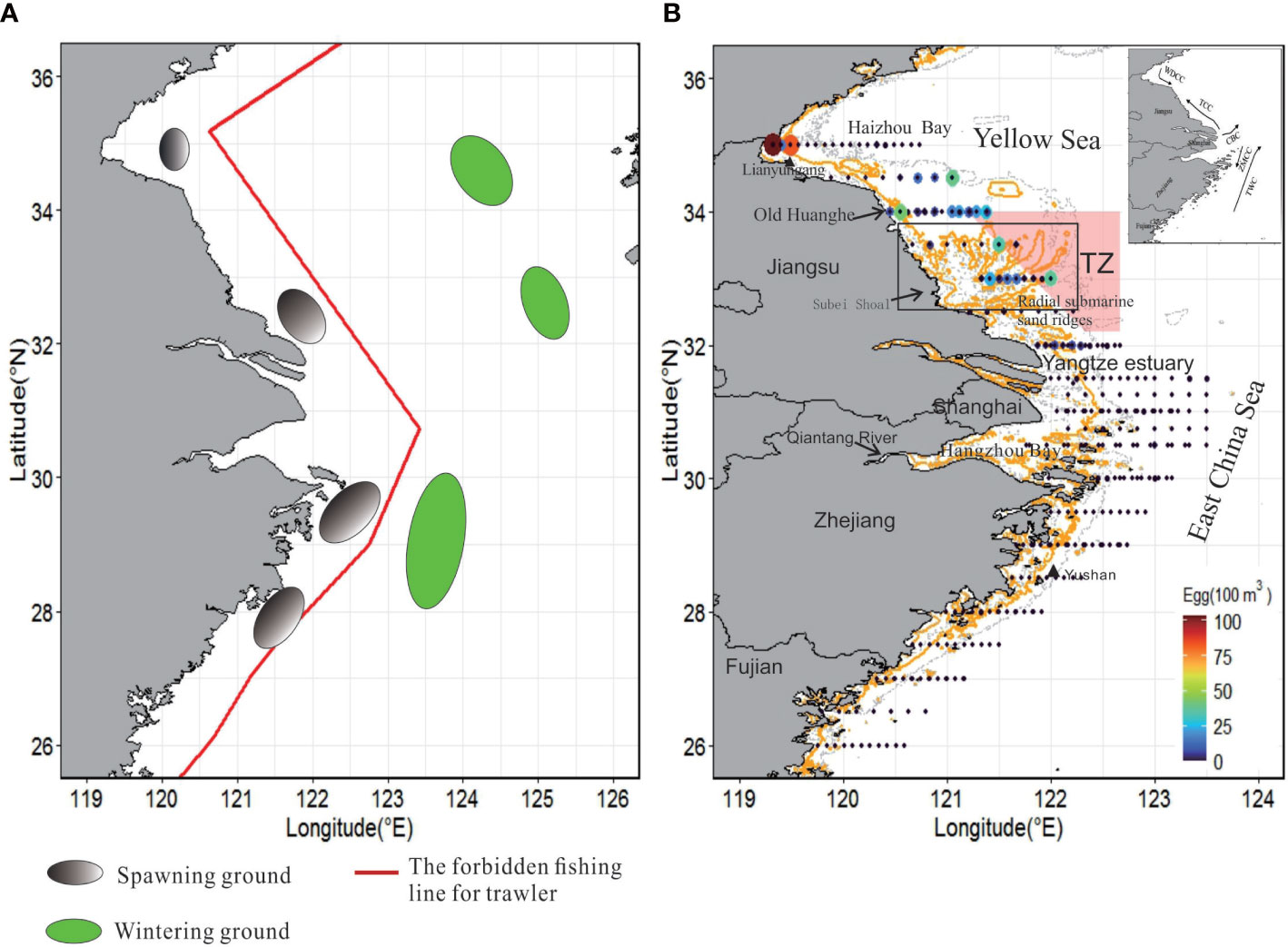
Figure 1 (A) The previous reported spawning grounds and overwintering grounds distribution of small yellow croaker in the coastal waters (Ren et al., 2020). (B) Geographical range and spatial distribution of fish egg abundance. The administrative regions within the survey range are displayed, including Jiangsu, Shanghai, Zhejiang, and Fujian. The survey results for stations and abundance in 2005 and 2008 reveal that the solid gold line is a 10 m isobath, the dashed gray line is a 5 m isobath, and the double dashed line is a 20 m isobath. The 10 m isobath along the Jiangsu coast reflects the existence of radial sand ridges. TZ represents the conservation zone for the small yellow croaker. The black triangle represents tide gauge stations. The coastal current system of China, wind-derived coastal current (WDCC), is shown on the upper right; TCC, tidal-induced coastal current; CBC, Changjiang bank current; ZMCC, Zhe-Min Coastal Current; TWC, Taiwan Warm Current.

Small yellow croaker begins spawning in spring, with their spawning period starting in mid-February and ending in late June, peaking in April and May (Xue, 2021). The spawning time of the small yellow croaker is closely related to their geographical location, indicating that local oceanographic changes may alter their spawning phenology and geographical distribution. However, a systematic study is lacking on the habitat and environmental preferences for the reproduction of the small yellow croaker along the East China Sea. Moreover, whether any geographical gradient change exists in the reproductive conditions still remains unclear. Culture experiments showed that the early-life development of the small yellow croaker was closely related to temperature, with larvae hatching from eggs within 60 h at 15-16°C (Chen et al., 2016). This suggests that during the first 60 h after spawning, the early horizontal dispersion of the small yellow croaker in the sea is mainly determined by the surface currents. It is significant to thoroughly understand the dispersal patterns associated with the spawning-aggregation formation and the identification of pre-spawning and spawning sites in response to spawning site planning and natural resource management.

Given the sensitivity of species to changes in environmental conditions, assessing the relationship between the egg abundance of the small yellow croaker and explanatory environmental variables in a region is key to determining the driving force of changes in spawning sites. This can be achieved through sophisticated statistical techniques and hydrodynamic modeling. Machine-learning methods, such as random forest (RF) models, are rather common among species distribution models (SDM) to explore the relationship between the occurrence or abundance of organisms and environmental factors. For example, such models have been employed to assess the effects of climate on the spatial and temporal distribution and abundance of terrestrial animals, plants, and marine organisms (Peters et al., 2007; Evans et al., 2011; Bouchet et al., 2017; Mazur et al., 2020). Moreover, RF analysis techniques represented excellent predictive performance in investigating small samples of threatened/declining species and/or rare species (Li et al., 2017; Siders et al., 2020).

The Lagrangian transport model provides an important perspective for studying the early distribution and influencing mechanism of marine organisms. It has been widely used to simulate the dispersal of plankton, including planktonic fish egg and larvae (Mariani et al., 2010; Suca et al., 2022). Particle traceability has received attention owing to its capability to identify spawning sites of fish populations. For example, Christensen et al. (2007) explored the methodological and implementation issues concerning spatial, temporal, and combined spatio-temporal backtracking. They illustrated the retrieval of the lesser sandeel (Ammodytes marinus) larvae in the North Sea and predicted the potential hatching areas from the perspective of biology. Bauer et al. (2014) tracked herring larvae of 6-10 mm in length back to their hatching sites; they also compared the model-identified spawning areas with the earlier field findings. In addition, transport models have been more frequently utilized to study the connection between spawning and larval sites and explore the mechanisms of retention, dispersion, and survival of larval and juvenile fish. Research on the movement of fish eggs and larvae in water plays a vital role in revealing the early life of fish and the environmental influence mechanisms of their resource dynamics.

This study was designed to identify the prioritized protection areas by quantifying the dispersal of eggs using the Lagrangian model. We also revealed whether the spawning timing was regulated by the local biophysical environment and whether spawning stock chose shallower area habitats with favorable growing conditions for offspring during the spawning season at different latitudes. To assess these objectives, this study (1) compared potential spawning areas and hydrography conditions along the near shores off ECSZ over time, (2) explored the association between the abundance/occurrence probability and oceanographic variables at different time lag, and (3) assessed the effect of current transport on the advection of eggs.

Materials and methods

Study area

The continental shelf of the ECSZ is a relatively open shallow marginal sea in the western Northwestern Pacific Ocean. It extends from 35°05’N to 22°N, covering four provinces and cities, Jiangsu, Zhejiang, Shanghai, and Fujian. The coast of the ECSZ is long and tortuous with diverse types, generalized divided into plain coast and mountainous and hilly coast. Complicated geographical and oceanographic characteristics directly affect the productivity level of this area.

Plain coasts are mainly distributed in Hangzhou Bay and the northern area, especially in the Yangtze River Delta. The Yangtze River is the largest river in China and the third-largest river globally, with an annual runoff as high as 9.0×1011 m³ (Zhao et al., 2021). According to recent studies of freshwater fluxes and long-term model simulations driven by climatic and real-world forces (Wu et al., 2014), the Yangtze River plume follows three pathways: It extends to the northeast coast in summer and southward along the coast in winter. In addition, the Stokes drift is induced by the coastal tides in Jiangsu Province. In summer and autumn, a small plume turns to the left and extends along the Jiangsu coast in the direction opposite to that of the coastally trapped wave. The mixed hydrodynamic processes in diluted water and the adjacent waters of the Yangtze River Estuary have brought about significant changes in environmental gradients and nutrient enrichment and provided essential habitats, foraging ground, and spawning sites for fish of different ecological types, such as migration and estuarine settlement.

The coast of Jiangsu is a muddy plain, where forms a watershed-like radial sand ridge, represented as a unique geomorphic type. It extends from the Sheyang River estuary in the north to the Yangtze River Estuary in the south. It is 200 km long from north to south and 140 km wide from east to west. There are more than 10 large groups of subwater sand ridges distributed in long strips, radiating to the north, northeast, east, and southeast directions of the 150° sector. Some of the sand ridges are exposed to the water surface at low tide. The radial tidal current field is the driving force for their formation and maintenance (Chen et al., 2019). According to the characteristics of the seabed topography, the western sea near the land is relatively flat, and the hydrodynamic environment is dominated by the coastal and tidal currents in northern Jiangsu. The topography and hydrodynamic environment in the eastern offshore area are complex. From May to July each year, the northeastward current is formed under the joint action of tidal currents and coastal currents in northern Jiangsu, as well as wind currents driven by the southeast monsoon (Dong et al., 2018).

To the south of Hangzhou Bay is mostly the cape-bay coast. According to long-term observation, the shelf current system off the coast of Zhejiang and Fujian comprises three parts: Taiwan Warm Current (TWC), Yangtze River diluted water, and Zhe-Min Coastal Current (ZMCC). TWC exists year-round along the coast of Fujian and Zhejiang in China and flows northward along the 50-100 m isobaths (Zeng et al., 2012). TWC is characterized by high temperature (>20°C in May) and high salinity (>33.5 in May). Its onshore branch originates from the Taiwan Strait, and its intensity is controlled by the discharge of the Taiwan Strait and Kuroshio branch in northeast Taiwan (Wang J. et al., 2020). The pathways and extent of invasion vary with seasons. The flow axis of the invasion oscillates seasonally, and the advance could reach the vicinity of the Yangtze River Estuary (31.5-32.5°N). The location and invasion extent of TWC will affect the local water mass structure.

The hydrological characteristics of the ECSZ have a significant effect on the abundance of the small yellow croaker. From February to June per year, numerous small yellow croakers congregate in the shallow water for reproductive activities. Their aggregation is closely relevant to the high productivity along the coast, the chlorophyll (Chl)-rich waters formed by upwelling along the Zhejiang coast, the plume of the Yangtze River, and the tidal movements in the Subei Shoal. Moreover, these areas provide favorable environmental conditions for the development of fish eggs and larvae. Subei Shoal is the most important spawning site for small yellow croaker, owing to its unique topography of radial sandbars: the water mass in the central area of the Subei Shoal is mainly controlled by two currents, i.e., the forward tide from the East China Sea and the rotating tide from the South Yellow Sea (Yan et al., 2016). Due to the convergence and divergence of the two tidal waves, the water flow is slow or stationary, forming the “two-water phenomenon” of the sand ridge and tidal trench. The water flow is more urgent in the tidal ditch trench, and the reproductive population receives water stimulation to ovulate. In contrast, the water flow at the sand ridge is relatively slow, conducive to the retention and settlement of organisms. Most importantly, the abundance of zooplankton guarantees the prey for larvae and juveniles.

Sampling

In this study, small yellow croaker eggs were collected in the ECSZ and the South Yellow Sea on 6 cruises from mid-April to mid-June at a monthly interval in 2015 and 2018 (Table 1). We utilized a grid of above 114 stations between Fujian (24°00′N) and Jiangsu (35°00′N), covering variable distances from onshore to a maximum of 142 km offshore at depths of <70 m. Due to the large latitude span (11 latitudes), we divided the surveyed area into Jiangsu, the Yangtze River Estuary, Zhejiang, and Fujian and then set up 23 transects (Figure 1B). To ensure synchronized investigations in each region, each survey ship was responsible for two adjacent transects, while in the Zhejiang region, we increased the number of surveyed ships. Each transect was investigated by one of the ships. Each survey was conducted around the full-moon phase for approximately 1 to 2 days. Samples were collected using horizontal tows (0-3 m below the water surface) of plankton nets (0.505 mm mesh size, 130 cm diameter, and 600 cm length) at an average speed of 2 knots for approximately 10 min. The mouth of plankton nets was equipped with a flowmeter to estimate the sampled water volume. The ichthyoplankton were immediately preserved in 5% formalin.

TABLE 1

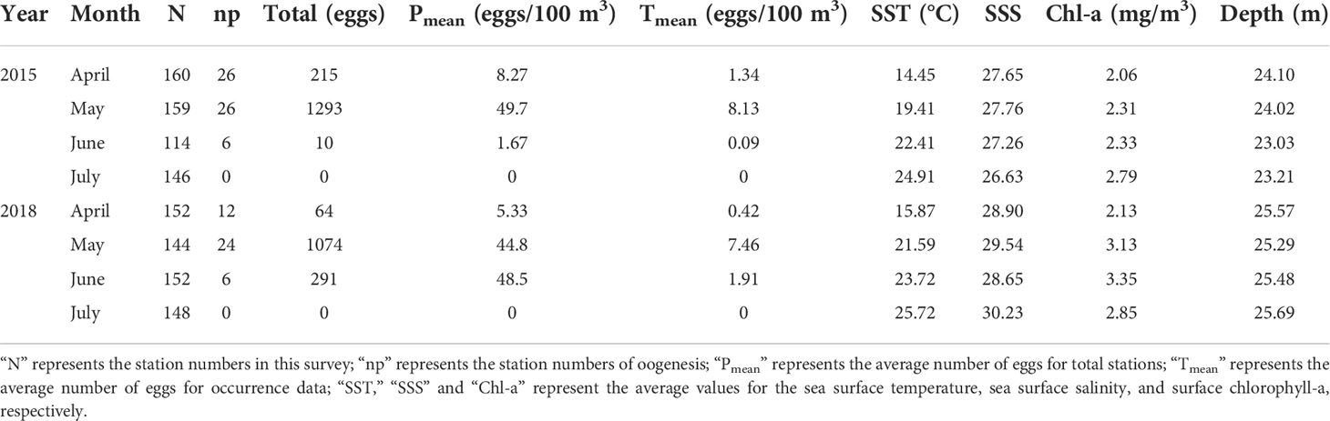
Table 1 Summary of variables of this study, including information on the surveyed stations, eggs, and hydrological variables, covering two distinct periods of 2015 and 2018.

Environmental data

The environmental data in this study were obtained from the Copernicus Marine Environment Monitoring Service (CMEMS¹). We downloaded the data on average daily temperature, salinity, Chl, ocean current, and wind field for the researched area (Table 1). Among them, data on temperature, salinity, and ocean currents came from a global reanalysis product named L4 level (product ID: GLOBAL_MULTIYEAR_PHY_001_030), which presented dedicated projection and spatial resolution. It was defined on a standard collocated grid at 0.083 degrees (~8 km). Parameters were interpolated from the native grid model.

Daily means of sea-surface chlorophyll-a (Chl a, mg m^-3) were also obtained for the identical region and time period with a spatial resolution of ~4 km. Products were based on a multi-sensor algorithm approach and were provided at level L4. An interpolation procedure was applied to fill in the missing data. We selected REP products (product ID: OCEANCOLOUR_GLO_CHL_L4_REP_OBSERVATIONS_009_082), which were consistent multi-year time series produced via a consolidated and consistent input dataset. As such, they represented a much more solid dataset for long-term analysis.

Topographic variable data were derived from the General Bathymetric Chart of the Oceans (GEBCO²), a global topographic model integrating bathymetric data with a spatial resolution of 15 arc seconds. The terrain ruggedness index (TRI) provides a measure of seafloor complexity and highlights small changes in the seabed terrain (Pennino et al., 2019; Liu et al., 2022). It was derived from continuous bathymetry using the raster package (Hijmans, 2020) in R (R Core Team, 2020). Oceanographic variables at 5-meter depth and topographic variables were extracted for each position and date of the survey dataset. All variables were downscaled using bilinear interpolation to match our egg data.

Model building and performance evaluation

We employed a zero-altered (or hurdle model) RF model to handle the excess zeros in the response variables (Montesinos-López et al., 2021). Zero-altered models are hybrid models with 2 parts: the binary part and the truncated count part. In the binary part, a conventional binary RF model was used to model the occurrence (SDM); in contrast, the truncated count part was modeled using an RF model to estimate relative abundance with a new splitting criterion based on the zero-truncated lognormal distribution (SAM) (Mi et al., 2017; Montesinos-López et al., 2021) (Table 2). We modeled the positive fraction for eggs because the limited number of available presence observations of eggs might hinder capturing environmental signals impacting the higher abundance aggregation. Models were fitted using spatial RF machine learning (Wright and Ziegler, 2017; Benito, 2021) via the ‘spatialRF’ R package (Benito, 2021). RF is an ensemble of several tree predictors such that each tree relies on randomly and independently selected features but has the same distribution (Breiman, 2001), which achieves greater predictive capability than other statistical models (Smolinski and Radtke, 2017; Friedland et al., 2021). The RF method is described in detail by Breiman (2001).

TABLE 2

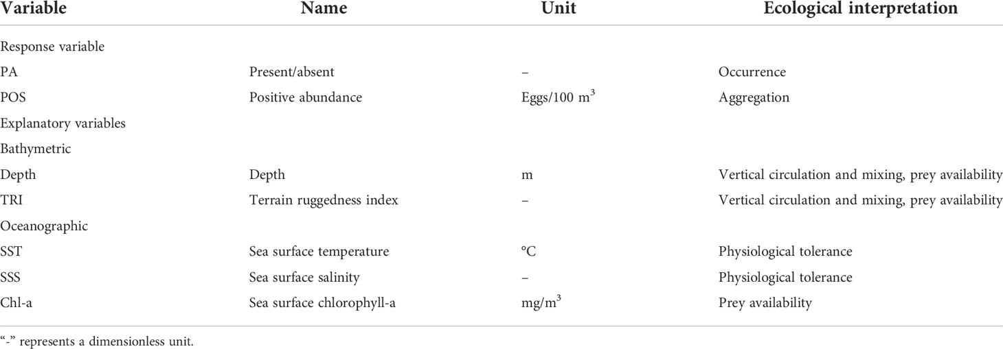
Table 2 Summary of the egg-predictor used in the establishment of the occupancy and abundance-habitat models, covering information on the description, unit, and potential ecological meaning.

The ultimate goal of spatial RF is to minimize the spatial autocorrelation of the model residuals. Before fitting the model, the independent variable set was tested for multi-collinearity among the predictors, and variables were eliminated using ‘auto_cor’ and ‘auto_vif’ functions through different criteria (bivariate R squared and variance inflation factors). From these reduced predictors, the final model variables were selected utilizing the model selection criteria with correlation coefficient |r| < 0.7 and VIF < 4, including sea surface temperature (SST, °C), sea surface salinity (SSS), Chl, depth, and TRI. The latitude variable was excluded due to its high correlation with SST (r > 0.7). In addition, considering that spawning could be affected by the environmental conditions during the previous days (Casaucao et al., 2021), a set of models was created corresponding to a time lag of 1 to 3 days before egg sampling. These variables were obtained through the reanalysis of daily mean data; the data were prepared in much the same approach as reported by Liu et al. (2022).

The Euclidean distances of the sampling locations were used to represent geographical measures of proximity and connectivity between observation points; distance thresholds (0 km, 10000 km, 20000 km, and 30000 km) were selected as neighborhoods at which the RF model would determine the spatial autocorrelation of the residuals. We started the model with non-spatial RF based on the default hyperparameter values provided by the ranger (Wright and Ziegler, 2017). If the spatial autocorrelation of the residuals for non-spatial RF was highly positive for the pre-specified neighborhood, we fitted the spatial RF models using Moran’s eigenvector maps to minimize the spatial correlation of the model residuals (Dray et al., 2006).

The performance of the model was assessed using a cross-validation (CV) procedure. At each iteration, 75% of the data were randomly partitioned as the training dataset, and the remaining 25% were kept for evaluation (Rullens et al., 2021). We repeated 50 iterations of the selected model to capture the effect of the stochasticity of the algorithm on the variable importance scores, predictions, residuals, and performance measures. The CV-based median values of root mean square error (RMSE) and R-square (R²) were used to calculate the predictive performance of the occurrence and abundance models. They were further compared with the different time-lag models, respectively. The RMSE and R² are calculated as follows:

$\begin{array}{ll}\text{RMSE}=\sqrt{\frac{1}{m}\sum _{j=1}^m{\left(\widehat{y}\left(s_j\right)-y\left(s_j\right)\right)}^2}& (1)\end{array}$

$\begin{array}{ll}{R}^2=\left[1-\frac{SSE}{SST}\right]& (2)\end{array}$

where ŷ(s_j) is the predicted value at CV location s_j, and m is the total number of CV points. RMSE is close to 0, indicating a perfect model. In R², SSE is the sum of squared errors at CV points, and SST is the sum of total squares. A coefficient of determination close to 1 implies a perfect model.

The relative importance of predictors for RF was calculated based on the change in the prediction error. A randomization approach was repeated 50 times to generate the median values of variable importance. A higher variable importance value indicates that the variable has a greater influence on the model (Xu et al., 2022). The response curves of the two most important environmental variables for each month were plotted to show the importance of the respective variable in explaining the observed egg distribution.

Backtracking model for particles

Regional Ocean Modelling System (ROMS) was used to simulate current data on the spawning sites, which was driven by tidal forcing and wind forcing. The simulated range was 119°-125°E and 27°-36.5°N. The simulation period started on April 1, 2018 and ended on June 30, 2018. The model was constructed with a horizontal resolution of 1/20°, about 6 km, and was uniformly divided into 20 sigma layers vertically. To improve computational efficiency, the model adopted 30-core paralleled computation. The step size of the outer mold was 3 seconds, and that of the inner mold was 60 seconds. The model output full-field 3D data once per hour and surface data once every half hour. Because the simulated site was a shallow sea with tide-controlled waters, the boundary water level drive was adopted. The boundary water level was predicted using the harmonic constant output from the TPXO9 global tidal model (Egbert and Erofeeva, 2002; Núñez et al., 2020). We also used the ERA5 reanalysis dataset provided by European Centre for Medium-Range Weather Forecasts (ECMWF³) as the atmospheric forcing to account for the wind-driven current. The data were available every five days. During the simulation, the wind field was filled using linear interpolation. The model-derived tidal level data for April 2018 were nearly identical to the measurements obtained from the tide gauge station, and the model in question was generally reliable and usable (Supplementary Figure S1).

The three-dimensional fields of hourly velocity averages from April to June 2018 were used to force the Lagrangian transport model. The release location of particles corresponded to the RF prediction of the high-density distribution of fish eggs. We used backward simulation analysis to trace the origins of particles and explore the potential spawning range. A total of 2000 particles were released, and the release time was the sampling day with the highest abundance in the surveyed month, i.e., at 12:00 a.m on April 22, 2018, May 18, 2018, and June 13, 2018. The actual survey time varied slightly among stations. Moreover, the small high-density areas were concentrated in only 2-5 stations with an inter-distance of less than 30 nautical miles (maximum survey time difference of 3 h). Therefore, we believed that ignoring the time difference would have little impact on tracing the spawning locations. According to the culture experiment of the small yellow croaker, the hatching time of eggs was about 50-60 h. For this reason, the model was run for a maximum of 60 h, and its outputs were stored every 20 min, including the location, latitude, and longitude of each particle at each time step.

Priority protection analysis

The model with the greatest R² value for different lag days was selected to predict the occurrence and relative abundance of eggs within the hydrological environment data. In order to create a fine-scale and spatially continuous prediction surface, the environmental data from our sampling area were made into a raster layer with interpolated values of 200 × 300 grids (1.35´×2´) using Kriging interpolation (Nychka et al., 2017; Hijmans, 2020). Hotspot analysis was performed to identify the spatial patches defining potential spawning areas. The priority protection index (PPI) was used to identify priority areas for the conservation program (Mi et al., 2017), which combined the predictions of SDM and SAM. PPI provided an integrated view of the spatially and temporally explicit occurrence and abundance indices. Biologically, PPI represented the areas important for the presence of spawners and the maintenance of large reproductive numbers (Estrada and Arroyo, 2012). It is calculated through the following equation for each site:

$\begin{array}{ll}PPI=\frac{P\times A}{max\left(P\times A\right)}& (3)\end{array}$

where PPI denotes the priority protection index (that is, a pixel index from 0 to 1 represents the priority of conservation), P is the probability of occurrence predicted from SDM, and A is the relative abundance predicted from SAM.

We recalculated the backtracking priority protection index (BPPI) by incorporating the dispersal range of eggs according to the backtracking model. From April to June, the selected release areas were [122°E,122.3°E] x [31.9°E,32.1°N], [119.3°E,121.4°E] x [34°E,35°N], and [120.5°E,121.05°E] x [34°E,34.5°N], corresponding to the core distribution range of the relative abundance of eggs. The particles in each cell within the range (defined as source cell Cell_inti) were randomly assigned in proportion to the relative abundance. For each season, Cell_i located by the transport pathways at the particle inversion of 24 h, 48 h, and 60 h was obtained every 2 hours, and the number of particles from different sources of Cell_inti was calculated. Then the relative abundance of Cell_i was expressed as follows:

$\begin{array}{ll}{A}_i=\frac{Ncel{l}_i}{\max (Ncel{l}_{inti})}\hspace{0.17em}x\hspace{0.17em}\text{max }\hspace{0.17em}\left(A_{inti}\right)& (4)\end{array}$

where A_i is the abundance index of cell_i located by transport pathways. N_cell is the number of particles in the i cell of the transport pathways. Ncell_inti is the number of particles in the cell at the time of particle release.

$\begin{array}{ll}\text{BPPI=}\left\{\begin{array}{cc}PPI,& cel{l}_{inti}\\ \frac{P_i\hspace{0.17em}\text{x}\hspace{0.17em}{A}_i}{\max \hspace{0.17em}(P_i\hspace{0.17em}\text{x}\hspace{0.17em}{A}_i}& cel{l}_i\end{array}\right\}& (5)\end{array}$

Finally, according to the BPPI value of each cell, the distribution area of the spawning site was plotted, and the hotspot distribution range was determined with BPPI > 0.7 as the threshold. The hotspot area predicted by the RF model and integrated with the tracking model was calculated respectively.

Results

Distribution of eggs

Table 1 summarizes the survey results of the planktonic eggs from April to July. The egg density at occurrence stations varied within the range of 0.04-103 eggs/100 m³. The greatest number of eggs was found in May; the average density of eggs at occurrence stations was 49.7 eggs/100 m³ in 2015 and 44.8 eggs/100 m³ in 2018. The egg density in April and June represented a large inter-annual change; the total number and average density of eggs in April 2015 were both greater than those in 2018. As for June, the changing trend for the indicators was opposite to that of 2018. No eggs were found in July.

The eggs occurring in 2015 and 2018 were analyzed. During the investigation, the egg density in the waters to the south of the Yangtze River Estuary was extremely low. No egg was observed in the waters of Fujian, and only minimal eggs occurred in the section of 30°N in the waters of Zhejiang. Numerous eggs were mainly distributed in the Jiangsu sea area, with the largest number in the coastal area of Haizhou Bay. The egg density gradually decreased with the extension towards the continental shelf. Eggs were mainly concentrated in the north-central area of Jiangsu Province, especially in the 33°N and 34°N sections.

Environmental characteristics

High Chl concentrations (>3 mg/m³) were mainly found in the coastal waters of the continental shelf, presenting a high concentration along the coastal waters and a low concentration offshore, especially in the Yangtze River and Huaihe River estuaries (Figure 2A). The concentration and range of Chl fluctuated with the month, and the high Chl concentration (>3 mg/m³) in April was limited from the Yangtze River Estuary to the northern coast of Zhejiang Province. In May, High Chl concentrations extended to the whole continental shelf; and a higher Chl concentration area (>5 mg/m³) appeared along the northern coast of Jiangsu Province. In June, elevated Chl concentration with an extended range was found, with the highest concentration (>6 mg/m³) in the coastal waters of northern Jiangsu Province. Chl represented a relatively low concentration but a large extension range in southern Jiangsu. Chl concentrations gradually increased with the elapse of the month due to the rising temperature and nutrients. The Chl concentration peak along the Jiangsu coast might be related to the change in wind direction as well as the transportation and distribution of terrigenous materials brought about by the Yangtze River and the northern Jiangsu coastal current.

FIGURE 2

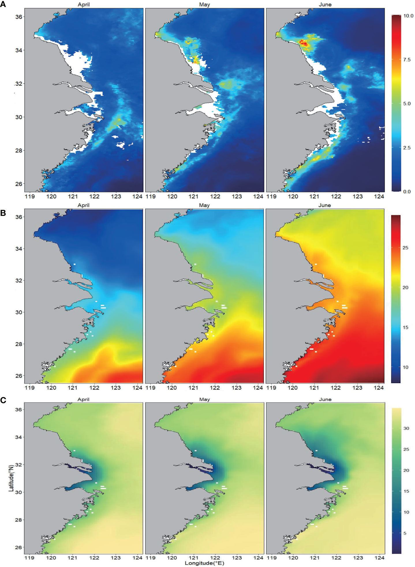
Figure 2 Monthly means of (A) chlorophyll-a (Chl-a), (B) sea surface temperature (SST), and (C) sea surface salinity (SSS) from April to June from 2015 to 2018.

SST showed the maximum value in April in the southeastern part of the ECSZ (above 21°C) (Figure 2B). Coastal waters presented relatively low temperature, which was lessened from low to high latitudes, possibly induced by TWC, coastal current, and diluted water diffusion. The temperature along the Jiangsu coast ranged from 9 to 15.2°C. In May and June, the ocean temperature gradually increased from 13.2 to 20.8°C and from 18.7 to 24°C, respectively. The temperature in coastal waters was higher than that of the outer sea in all seasons, while the salinity showed the opposite pattern (Figure 2C). This might be induced by the left turn of the outfall of the Yangtze River diluted water and its extension along the Jiangsu coast. This also provided important nutrient sources for the frequent algae blooms in this area.

Model evaluation and variable importance

The RF model was employed to evaluate the performance of the lag model and its predictability on the sampled dataset (Table 3). Without considering the lag effect, the model represented a slightly changing performance and high fitting each month. Its binomial part explained 87.7%-90.9% of the out-of-bag variance (R²), while its abundance part explained 71.1%-85.7% of R². Considering the lag effect, the correlation between fish eggs and environmental factors was analyzed through different time lags. R² and RMSE values indicated that the optimal model changed with the month. Lag1 presented the highest explanatory power for R² and RMSE in April, while it was Lag2 in May and June. For the abundance model, Lag2 represented the greatest explanatory power for R² and RMSE in April. In May, the R² and RMSE selection models were different, which were Lag0 and Lag1, respectively. In June, the model with the maximum explanatory power was Lag2. As such, we speculated that the location of oogenesis and abundance aggregation were closely related to the parental selection of spawning sites, and the lag days might reflect the spawning time.

TABLE 3

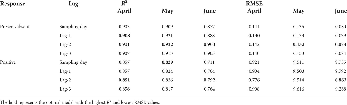
Table 3 Model performance evaluations for occupancy and abundance habitat models with a maximum time lag of 3 days based on R² and RMSE using RF analyses from April to June.

Based on the presence-absence response variables, the importance of various environmental variables in SDM and their influence on spatial distribution were explored using the error increment (Figure 3). The results from 50 simulations identified that SST and SSS were the two most important variables, producing the greatest error variation from April to May, followed by TRI, containing zero value and indicating the existence of uncertainty. In June, fewer fish eggs were found, and the variation range of environmental factors was poor, resulting in the failure to identify the most important environmental variable(s).

FIGURE 3

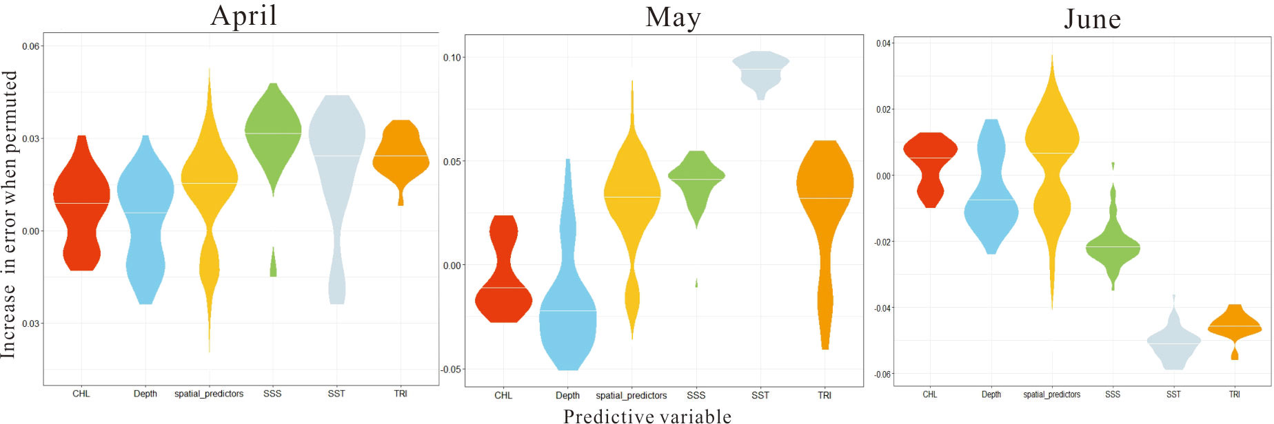
Figure 3 Variable-importance scores between predictors from April to June obtained by repeating SDM execution 50 times.

Response curve analysis revealed the response of occurrence probability to environmental variables (Figure 4). Overall, the occurrence probability showed a negative nonlinear trend to temperature and salinity. Regime shift existed in both temperature and salinity, and the occurrence probability dropped slowly with increasing salinity under low-salt conditions but plummeted above the transition point (27 in April and 29.5 in May). At low temperatures, temperature showed a positive correlation with the occurrence probability. In April and May, a turning point was observed at 16°C and 19°C, respectively. At high temperatures (above 16°C in April or above 21°C in May), the occurrence probability was extremely low. The results indicated that the spawning behavior of the small yellow croaker showed poor tolerance to temperature and salinity.

FIGURE 4

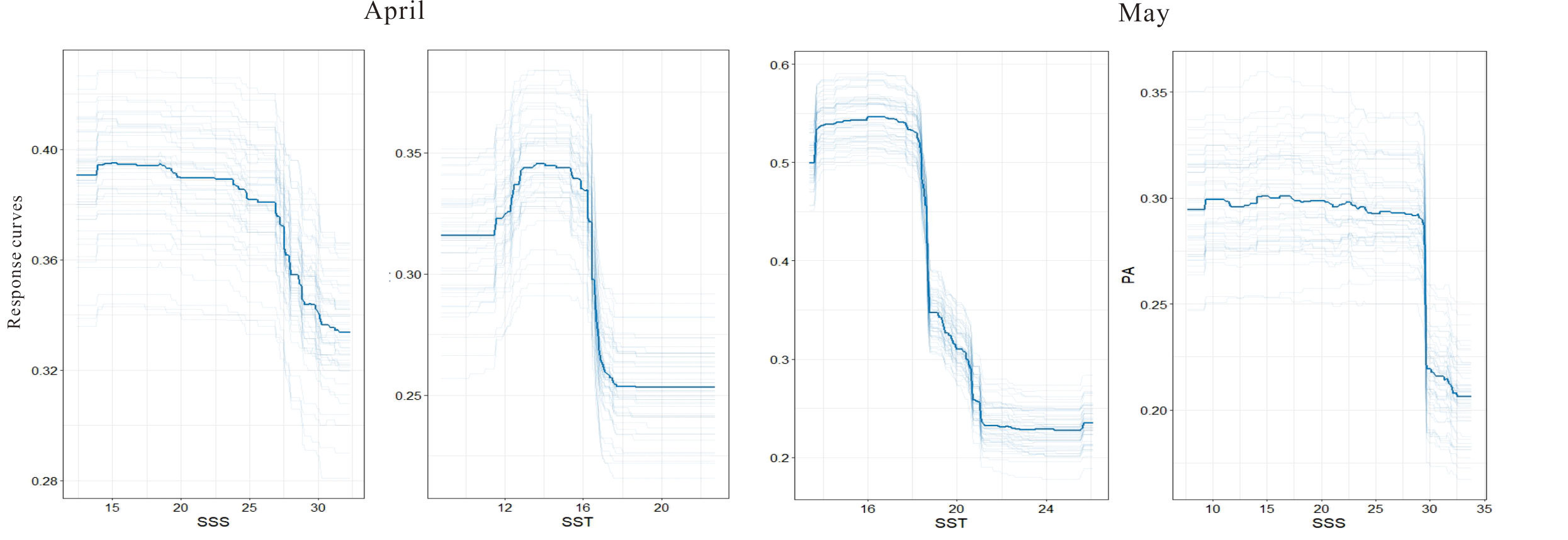
Figure 4 Response curves for the two most related environmental factors on the egg distribution of the small yellow croaker from April to May by repeating the SDM execution 50 times. The bold solid line is the median response curve, and the light solid line is the response curve obtained by repeating each model.

According to the analysis of the positive abundance response variable (Figure 5), in April, Chl was the main factor affecting the aggregation of egg abundance, followed by TRI and SST. In May, the most significant variable was SST, followed by Chl and TRI. Only Chl showed the greatest effect in June. It could be seen that the effect of Chl concentrations on egg abundance lasted throughout the spawning period. As can be seen in Figure 6, in April, the high-abundance regions of fish eggs were mainly concentrated in the low-Chl-concentration area; when exceeding 1 mg/m³, the Chl concentration represented a significantly decreased influence on egg abundance. The influencing trend of TRI on egg abundance was similar to that of Chl concentration. The fish egg abundance was relatively high in the relatively flat seabed but was relatively low in sea areas with higher roughness. In May, with the improvement of Chl concentration (2.5 mg/m³), the abundance of fish eggs also increased significantly with a nonlinear trend. Upon reaching a certain threshold, the abundance of fish eggs began to stabilize; however, it reached the highest level within a narrow optimal range of Chl concentration and then gradually decreased. The effect of temperature on fish eggs was opposite to that of Chl. When SST was below 15°C, the abundance of fish eggs was higher (above 15 eggs/100 m³). With the increased SST, the abundance of fish eggs dramatically decreased. When SST was higher than 16°C, the egg abundance stabilized at a lower level. However, there was still a secondary peak of egg abundance at 19-20°C, significantly different from that at the highest level. In June, Chl concentration and water depth exerted a gradient effect on egg abundance, which was the lowest in sea areas with Chl concentrations below 2.5 mg/m³. As the Chl concentration rose, the egg abundance increased dramatically; when it exceeded 3 mg/m³, the egg abundance basically remained stable. The waters with the greatest egg abundance corresponded to the maximum Chl concentration (above 6 mg/m³). In terms of the water depth, the high egg abundance was mainly concentrated in shallow waters less than 13 m in depth. However, when the water depth exceeded 17 m, a secondary peak of the egg distribution area was observed.

FIGURE 5

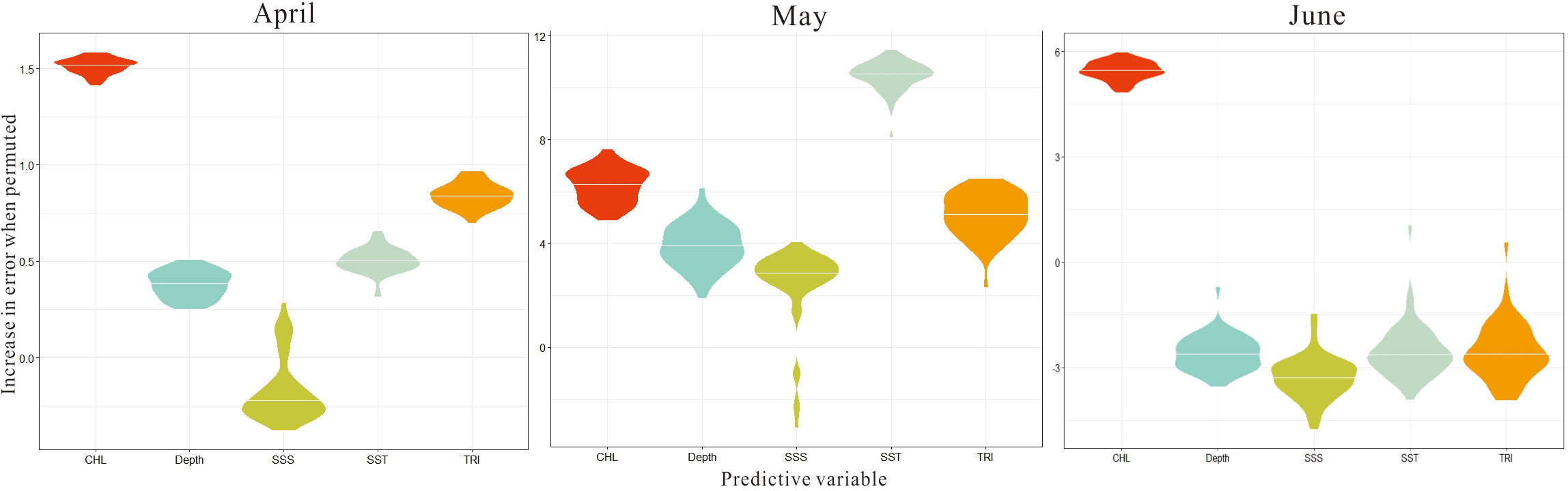
Figure 5 Variable importance scores among predictors from April to June by repeating SAM execution 50 times.

FIGURE 6

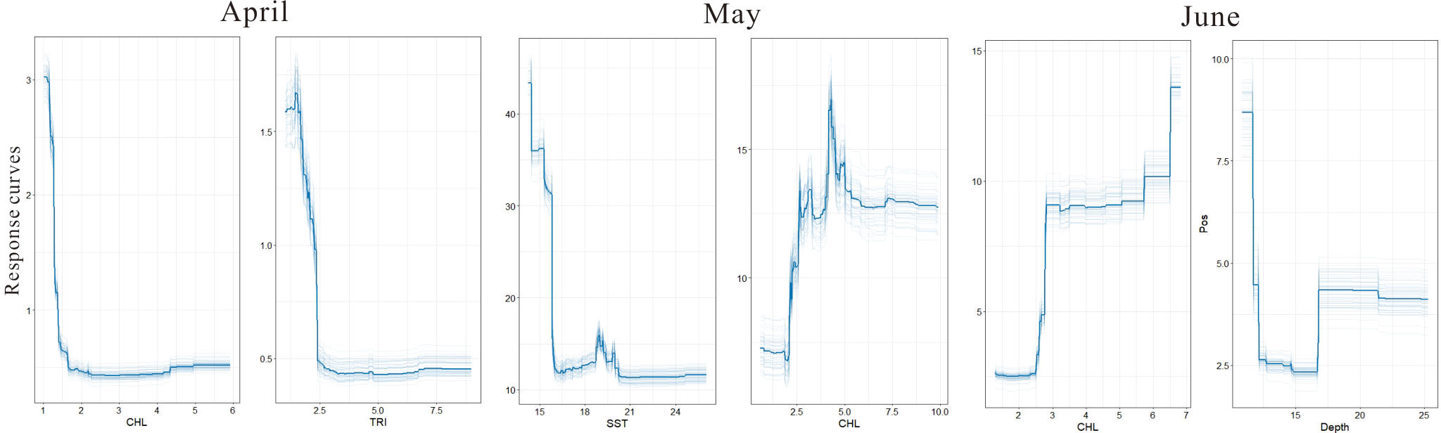
Figure 6 Response curves of the two most related environmental factors on the egg distribution of the small yellow croaker from April to June by repeating SAM execution 50 times.

Egg dispersal trajectories and conservation priority zone

The main results of simulated trajectories suggest that contribution of eggs produced within the released areas is predominant over the contribution from surrounding areas (Supplementary Figure S2). Figure 7 shows the spatial distribution of PPI of the spawning grounds of the small yellow croaker, presenting a predictable and consistent pattern. The conservation priority zone represented a concentrated spatial distribution and a changing location with the month. The zone with higher PPI (above 0.65) was mainly distributed in the southern sea area of Jiangsu in April, Haizhou Bay in May, and the central part of Jiangsu in June. Without considering the dispersion of fish eggs (Table 4; Figure 7), the largest area with PPI > 0.7 appeared in June (7,409.44 km²), while the smallest area (only 329.5 km²) was found in May. Through Lagrangian transport analysis, the potential spawning ground of the small yellow croaker might exist in the southeast of the sampling location. The dispersion pathways exerted different effects on the monthly BPPI, as shown in the enlarged area with BPPI > 0.7 each month (Table 4; Figure 8), and April presented the largest increase in BPPI, 1.24-1.43 times greater than before. The following month was May, with an increase of 32.57%-48.88%. We found the poorest increase of 5.2%-12.53% in June. The concentrated and small-scale distribution of spawning areas of the small yellow croaker enabled the marine conservation areas to provide convenient planning. However, the spatial location features varied with the month also indicated that temporal changes should be considered in the delineation of protected areas.

FIGURE 7

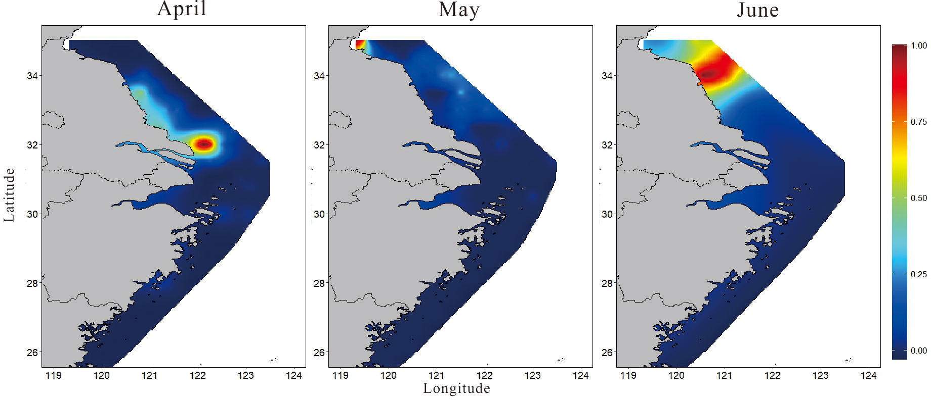
Figure 7 Spatial distribution of the priority protection index (PPI) for the spawning grounds of the small yellow croaker without concerning egg dispersion.

TABLE 4

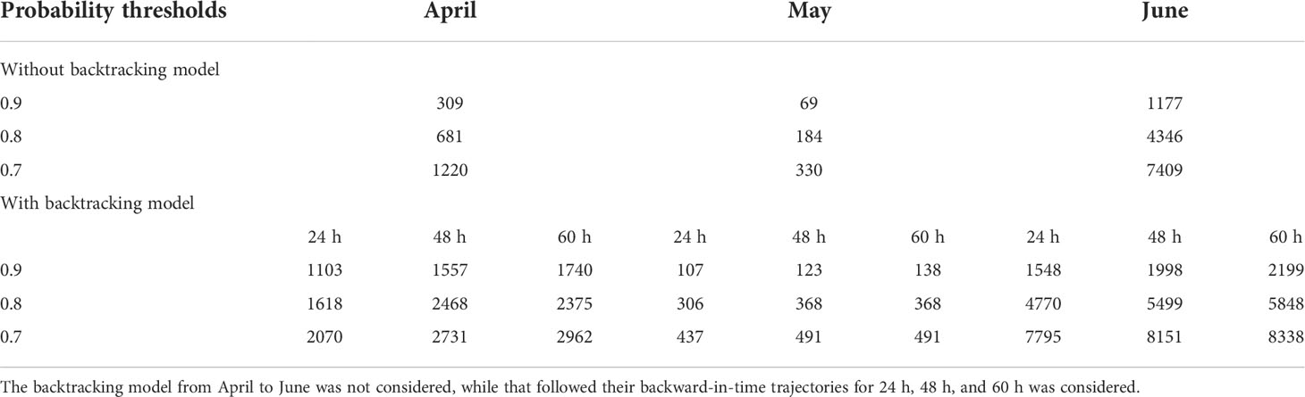
Table 4 Model-based estimates of areas (km²) in priority protection areas based on the probability thresholds of 0.7, 0.8, and 0.9.

FIGURE 8

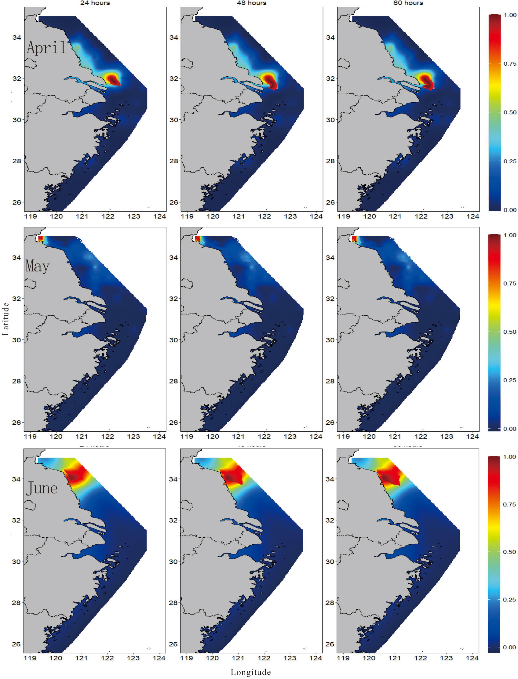
Figure 8 Spatial distribution of the priority protection index (BPPI) for the spawning grounds of small yellow croaker with 24 h, 48 h, and 60 h backward tracking of egg dispersion.

Discussion

In this study, RF was used to generate spatial predictions, but the spatial location of points (geography) was generally ignored during modeling. Spatial auto-correlation in CV residuals indicated that the predictions were possibly biased. Integrating variables related to geographical location (longitude and latitude) could upgrade model performances (Hengl et al., 2018). According to SDM and SAM results, when the time delay was 1 or 2 days each month, the correlation between egg density and environmental variables was high (Table 3). This indicated that before spawning, the parents might require suitable environmental conditions, such as high Chl-a concentrations and suitable temperature and salinity. For example, to increase the food availability of anchovy larvae, the Chl-a concentration 3 days before spawning was the most significant environmental variable to characterize the spawning site (Casaucao et al., 2021). The lag effect was also evident in other organisms at different stages. For example, in the South China Sea, the Chl-a concentration exerted a delayed effect of about 2 months on protozoa (Yu et al., 2019), which mainly depended on the nutrient levels and life stages of different organisms (Wang et al., 2021a; Wang et al., 2021b).

SST and SSS were the most important factors determining the spawning activities of the small yellow croaker. The temperature represented a smaller range of changes than the salinity, reflecting the strict environmental requirements for reproductive activities in habitats. Temperature can strengthen or inhibit gonad development and maturation by affecting the metabolic intensity of the fish, thus impacting fish spawning and hatching. The spawning time of many fish is determined by the surrounding water temperature before spawning, known as the famous “phenology” phenomenon in ecology. This phenomenon has been demonstrated in various migratory fish-monitoring programs or fish-farming experiments (Sims et al., 2004; Asch, 2015; Sydeman et al., 2015; Langan et al., 2021). The present study revealed that the temperature gradient changed with time or latitude at different spawning sites. The lowest temperature for the spawning grounds of small yellow croaker north of the Yangtze River Estuary was 11.5°C, and the habitat with high abundance was concentrated in the Lvsi Sea area at 12-15°C (average 13.3°C). According to a previous report (Chen et al., 2016), at a water temperature of 13°C, 70% of the gonad development of the parent fish could be observed in the “V” stage, and the incubation temperature of eggs was 14-15°C, which was in the higher water temperature range of egg distribution investigated in April. However, this temperature range only represented the minimum temperature at which the small yellow croaker could reproduce. In June, the spawning population of the small yellow croaker in the central Jiangsu sea required a temperature of 19-21°C. The water temperatures that address the thermal limits of reproduction provide physiological switches for the beginning and cessation of fish reproduction. Temperature can directly affect the initiation of spawning by promoting and inhibiting hormone synthesis, but the warmer temperature may cause the cessation of fish reproduction and a shorter spawning period (Motani and Wainwright, 2015; Spinks et al., 2021). A recent comparative study on fish identified that spawning adults and embryos had narrower thermal tolerance ranges, as reproduction and embryogenesis were the most thermally sensitive time for fishes (van Heerwaarden and Sgrò, 2021).

The diversity of spawning sites and wide heat tolerance of fish offer a higher probability of population continuation for fish with opportunist spawning strategies. The spawning strategy of small yellow croaker consists of obstinate strategy and the opportunist strategy. Most spawning individuals (53.67%) returned from offshore to the coast, where they were born to spawn at predictable times (Wang, 2021). In contrast, differences existed in choosing sites and exploring environmental variability for some spawning individuals, indicating their opportunistic reproductive strategies. Moreover, populations that combined the above two strategies could avoid extinction under severe environmental changes (LePage and Cury, 1997). In addition, the reproductive timing of the small yellow croaker also showed interannual variation, suggesting that energy and nutrient requirements could be improved to match the peak of seasonal resources through phenological plasticity. Phenological changes have also been increasingly recognized as a common response of species to ongoing climate change (Woods et al., 2021). Therefore, in order to enhance our understanding of the reproductive phenology of the small yellow croaker in their response to climate change, we need to comprehensively consider the environmental cues and intrinsic traits to enhance our perception of the timing of seasonal life events (Woods et al., 2021).

The Chl concentration was the main driving factor of egg aggregation in each month, showing that nutrition was an important factor influencing the parental selection of spawning sites. This is because spawning aims to provide a favorable foraging and feeding environment for larvae, and the Chl concentration is an indicator of primary productivity. The positive correlation between Chl and abundance is particularly significant in pelagic fish (Casaucao et al., 2021), whose seasonal variation affects almost all reproductive traits of sardines and even increases reproductive potential with improved primary productivity. The correlation is used to predict changes in the spawning habitat and frequency (Ganias et al., 2003; Reiss et al., 2008). The positive response of egg density to Chl concentration in May and June indicated the dependence of egg density on Chl. The larval stage (< 17 mm) of small yellow croaker feeded mainly on copepods (Chen et al., 2022), and thus the close correlation between spawning dynamics and Chl reflected an adaptive mechanism of improving progeny survival by matching spawning time to favorable environmental conditions during early development, consistented with the match-mismatch hypothesis. Low-salinity water exists in the coastal waters of Jiangsu Province all year round and contains a high concentration of terrestrial nutrients capable of significantly promoting the massive growth of phytoplankton (Su and Yuan, 2005; Zhu and Wu, 2018). This creates a suitable habitat for the spawning of the small yellow crocker (salinity < 30). The Yangtze River Estuary is adjacent to northern Jiangsu, between which the water exchange is frequent. The Subei coastal current carries terrestrial-sourced nutrients to the southeast, while the Yangtze River diluted water is transported to the north and strongly intersects with Subei coastal current, thus providing favorable conditions for phytoplankton growth. The seaward boundary of centers of high Chl concentration nearly matches the isohaline of the Yangtze River plume front. However, the influence of the residual water flow of the Yangtze River on the coastal water in northern Jiangsu is limited to the area south of 33.5°N, and the freshwater content of the Yangtze River covers 60%-70% of the total fresh water in the Subei coastal water in spring. In the area north of 34.5°N, terrestrial-sourced materials of rivers in northern Jiangsu are the most important sources of nutrients in the coastal water of northern Jiangsu (Zhu, 2018). Moreover, the high-nutrient water bodies in the coastal water of Jiangsu are considered the origin of marine disasters, e.g., the outbreak of Ulva prolifera. However, the Chl concentration exerts a non-linear negative effect on the egg abundance in April, implying that in April, the Yangtze River diluted water plume still maintains the turning characteristic in winter, and the main outlet quickly appears to the shore and moves southward. As the other part flows northward, the water force along the Jiangsu coast is weak, and the low water temperature, poor light, and lacking terrestrial material prohibit Chl growth. We captured the spatial pattern of surface Chl concentration and the geographic location of the phytoplankton bloom. Chl hotspots are distributed in a long curving band near 123°E and a northward boundary around 32°N. Wang et al. (2019) reported that the Chl concentration surged in late April and peaked in mid-June, consistent with our findings. Although the Chl concentration in the spawning sites in southern Jiangsu is lower than that at hotspots (29-30°N), salinity is a limiting factor in the reproductive activities of the small yellow croaker. For example, the salinity tolerance of the fish could reach 32-33.5 in the overwintering stage (Liu et al., 2020). Although salinity is important for gonad development and maturation in the spawning stage, reproduction needs low salt conditions (Chen et al., 2016). The waters with salinity lower than 30 in April are mainly distributed in the coastal areas of southern Jiangsu, Yangtze River Estuary, Hangzhou Bay, Zhejiang, and other narrow waters. These waters have a low Chl concentration, where the spawning grounds of the small yellow croaker are distributed, but the distribution hotspots are concentrated in the waters north of the Yangtze River Estuary.

The spawning stock of the small yellow croaker shows an obvious preference for the coastal environment, reflecting the influence of radial sand ridge on the distribution of fish eggs. The current velocity in the tidal gully of the radial sand ridge is relatively great, and fish swim to the tidal gully to receive the stimulation of the current for ovulation (He et al., 2015). The gentle flow at the tide ridge provides water mass with greater stability, allowing the formation and maintenance of prey aggregation. Along the coast of Jiangsu, the conflict between the Northern rivers of Jiangsu, the northern branch of the Yangtze River dilute plume, and the cold water mass of the Yellow Sea creates fronts, combined with unique topographical features, will generate areas of concentrated nutrient and plankton, and hence facilitate the retention mechanism for zooplankton and planktonic fish. Therefore, the radial sand ridge in Jiangsu Province is the optimum area for the survival of fish eggs and larvae, as well as the most concentrated complex spawning sites for various fish and shrimps. Another possible explanation is that this could be a unique complementary strategy based on predator avoidance. For example, in the Bay of Biscay, the predation risk is lower than that on the continental shelf. Anchovy spawn along the coast, and their larvae are horizontally transported offshore and then return to the coast, which is the migration mode with the least predation (Wang et al., 2021b). Coastal and offshore migration patterns also exist in the early life of the small yellow croaker by fully using the existing habitat. The small yellow croaker increases the survival rate of their offspring through lower-rate predation.

The oceanographic model showed a northwestward trajectory of egg transport, inconsistent with the effect of northerly winds on coastal currents (Supplementary Figure S3A). Although the northerly wind is strong, the resultant southward Ekman transport can only act on the water body surface. The water masses in the south of the Yangtze River Estuary are transported southward after exiting the estuary, but those in the north of the Yangtze River Estuary are transported northward (Supplementary Figure S3B). Although the northward flow speed is low, its long-term cumulative effect cannot be ignored, which causes warm, low-salinity surface water and the northwestern advection of Lagrangian particles along the coastal line. Through numerical simulation, Zhang (2014) believed that a distribution of a low-salinity belt with a salinity of less than 20 could be developed, close to that of the coastline from the outer Yangtze River Estuary to the east of Jiangsu Province; the salinity was higher than that of the Yangtze River Estuary but more than 5 lower than that of northern Jiangsu. This low-salinity zone co-sources with the low-salinity water of the Yangtze River and forms a low-salinity zone extending northward. Afterward, it forms a relatively strong front with the outer high-salinity water (Zhang, 2014). As a result, the eggs are confined to a narrow tongue of warm water. In the central region of Jiangsu, the northward transport between the Yangtze River Estuary and the northern sea area of Jiangsu gradually intensifies. Under the action of tidal energy gradient and positive pressure gradient force, the waters reaching the bank of the old Yellow River Estuary show offshore movement, moving eastward towards the outer part of the northern Jiangsu sea (Zhu, 2018). This results in the dispersion of the small yellow croaker eggs near the estuary to the sea in May and June with expanded distribution. The eggs in this part are confined to inshore waters south of 34°30’N and separated from the spawning sites in Haizhou Bay. In Haizhou Bay, the water is mainly transported southward along the coastline. Tidal energy gradient, advection, and friction constitute the main factors driving water transport southward. Due to the low flow velocity, we hypothesize that the distribution of the small yellow croaker in the bay is mainly affected by the local spawning grounds.

According to the traceability analysis, although advection may transport individuals to the northwest, the current velocity in the studied area is low, and the hydrodynamic force in the pre-hatching region exerts a minimal influence on the transport distance of eggs. The spawning grounds are mainly concentrated in the southeast sea of the survey station, and the maximum transport distance is less than 30 km after drifting at 13 cm/s for 60 h. In addition, eggs and larvae at different stages of development are found from the coast of Jiangsu to the Yangtze River Estuary, indicating that the area is an important spawning and nursery site for the small yellow croaker, and its condition plays a significant role in the replenishment of the small yellow croaker.

A major challenge in the conservation of aggregated complex spawning grounds for the small yellow croaker and other fish is the lack of data on the early life history. Most of the studies focused on a small portion of the geographic range of species. Wang X et al. (2020) identified the spawning grounds in Changjiang fishing ground and Zhoushan fishing ground based on environmental DNA analysis, however, the study area was mainly located in the south of Yangtze River Estuary. In this study, the special survey project of spawning grounds provides relatively comprehensive data for delimiting spawning sites in conservation areas. In addition, habitat degradation and loss pose threats to the function and sustainability of spawning grounds for aggregative spawning fish. In some cases, these habitats are particularly vulnerable to the expansion of marine space induced by local economic and social development, running counter to the objectives of fishery resource saving and ecological conservation. For example, spawning sites are often close to shorelines, which is an important feature for many teleost fish, and also attracts the development of ports or terminals. In fact, some enterprises have recently expanded a “Lvsi Central Fishing Port,” which may affect the edge of the spawning grounds of certain fish, including the small yellow croaker. However, the expansion project has minimized the loss of recruitment by avoiding the core spawning area.

Haizhou Bay is the spawning and nursery grounds for a variety of fish and economic invertebrates. Due to the enhanced fishing intensity in recent years, Haizhou Bay and its adjacent waters have represented deteriorated ecological environment, with the biodiversity and environment quality facing unprecedented threats. The core spawning area near the Haizhou Bay National Marine Park is accessible to fish, shellfish, shrimp, crab, cephalopod, shellfish, and diverse creatures such as echinoderms. However, numerous farming activities in the inshore area of Haizhou Bay caused damage to the marine environment of this area by producing a large amount of organic matter and wastewater during mariculture. This, in turn, led to the eutrophication of waters in Haizhou Bay. Apparently, the eutrophication and degradation of the coastal ecosystem in Haizhou Bay are closely related to mariculture. Since 2007, the large-scale outbreak of U. prolifera in the Yellow Sea, the largest green tide disaster globally, has been attributed to the laver farming areas along the coast of Jiangsu. Laver rafting was believed to provide an appropriate attachment base for the growth of U. prolifera (Gao et al., 2014), which occurred in late April and showed the fastest growth and proliferation rate in May. The green tide erupted from June to July (Ji et al., 2015), overlapping with the early life of the small yellow croaker on temporal and spatial scales. The influential process of the green tide outbreak on fishery resources was extremely complex. The green tide was reported to mainly affect the primary production process in the ocean and endanger the survival rate of the fish larvae through the food chain (Wang et al., 2019; Sun et al., 2022). Sun et al. (2022) regarded the outbreak of U. prolifera as an event to simulate the natural death of the small yellow croaker and indicated at least 10% of biomass and catch loss of the small yellow croaker in the case of the surging natural death. However, Chinese fishing vessels were prohibited from operating during the summer fishing moratorium from May 1 to September 15, except for longline and single gillnet fisheries. The occurrence, development, and prosperity of this period overlapped with the occurrence of green tide completely. Consequently, the green tide-induced damage to fish populations and marine ecosystems might be partially offset. Differently, another view has been put forward that although green tides increase the mortality of fish populations, they can provide food sources and spawning sites for many marine organisms, which complicates the interaction between green tides and the dynamics of fish populations, including the small yellow croaker (Sun et al., 2022). Undoubtedly, under the disturbance of the deteriorated ecological environment and human activities, the spawning grounds of the small yellow croaker are facing complex stress situations, and the habitat degradation or loss of local spawning grounds may impact the population level. The individual small yellow croaker may continue to spawn at the traditional sites, but changing sites may impair the health of the population. If aggregated spawning sites are moved to non-traditional spawning sites after disturbance, important links between spawning sites, larval transport routes, larval habitat, and adult habitat may be severed. Therefore, studying the habitat changing mechanism and the effect of the degradation of key spawning aggregative grounds on the aggregation formation, spawning success, larval survival, as well as the connectivity between spawning sites, nursery grounds, and adult habitat will be an important direction for our planning of priority conservation areas and sustainability of the small yellow croaker resource.

Recently, the Chinese government has been taking positive measures to press ahead with the regulation of coastal development. In January 2018, the government announced strict controls on new coastal reclamation projects (Yang et al., 2020). In addition, China is building a system of natural reserves with national parks as its main body. China is the first country in the world to propose and implement a redline system geared towards ecological protection. China has also identified certain priority areas under biodiversity conservation. In 2018, the marine ecological redline protection plan implemented in Jiangsu covered a total area of 9,676.07 km², including 16 fishery-restricted redline zones of 6,066.09 km², 62.80% of the total. While these new regulations are promising, it remains to be seen how they will be implemented and whether local governments can strike a balance between fishery resource conservation and local economic development. According to the priority of species habitat protection, we suggest that the spawning area of the small yellow croaker should be fully considered in the ecological red line area. As can be seen, from the location of the germplasm resource reserve and the distribution areas of eggs of the small yellow croaker in April, the place concentrated with fish eggs in the north of the Yangtze River Estuary is not classified as a germplasm resource reserve. On this basis, it is suggested to connect the existing reserves with the spawning areas in the south and west or set up a conservation corridor between them to expand the reserve area appropriately. In this way, 62% of fish eggs will be included in the reserve. The newly added reserve also covers the spawning populations of mullet, sole, and Scomberomorus niphonius, forming a better protection network. The coastal areas have been included for protection during the summer fishing moratorium in May and June. Nevertheless, it is recommended to focus on the damage of marine engineering and aquaculture to the spawning area habitat. Although the protection of threatened spawning fish habitats is a top priority, continued degradation of remaining habitats remains a risk to be overcome. In the long run, it is necessary to recover declining coastal habitats for the following habitat reestablishment for targeted species.

The identification of potential spawning sites in this study is limited to a horizontal survey, which may be improved by concerning the vertical distribution. It appears to be the correct assumption that the floating eggs of the small yellow croaker exist in the surface water column. However, if the current moves vertically or turbulent mixing is strong, the eggs are likely to be mixed into the middle and upper water column. Some fish eggs, such as those of sardines and anchovies, are always present in the first 5 m (Planque et al., 2007). The vertical distribution structure of fish eggs can be analyzed using modeling programs, which are very complex and usually requires consideration of egg density, size, turbulence caused by wind and tide, and vertical hydrologic structure (Petitgas et al., 2006). It is expected that the developments of the existing model will promote spawning habitat prediction.

Conclusion

Our study analyzes the egg drift of the small yellow croaker, assuming that the floating eggs are in the upper water masses. From a backtracking perspective, the spawning site and the adjacent area (the maximum drifting distance is 30 km) are the preferred spawning habitat due to the local biophysical environment and the related potential benefits. Moreover, the observed temporal patterns in the spatial distribution of spawning can be explained by the temporal changes in hydrographic conditions, which may substantially influence the final settlement locations of eggs and larvae. This reproductive strategy can ensure maximum dispersal and survival opportunities. Since hydrographic conditions are variable between years, which may cause geographical shifts for FSA into favorable areas, and then drifting floating egg locations vary in space and time. Therefore, we recommend that spatial and temporal dynamics be considered in FSA marine protection area (MPA) or MPA network design with strict management measures to achieve explicit ecological objectives. To track the impact of FSA MPA establishment on target populations, the fishery-dependent or fishery-independent data on fish populations require to be collected.

Data availability statement

The original contributions presented in the study are included in the article/Supplementary Material. Further inquiries can be directed to the corresponding authors.

Author contributions

FH and JC designed the study. LLY, MX, YZ, JT, and YDZ collected the data. ZL and YJ performed modeling and statistical analyses. ZL wrote the original draft. ZL, YJ, and LPY contributed significantly to the drafting of the manuscript. JC was involved in the funding acquisition. All authors contributed to the article and approved the submitted version.

Funding

This work was financially supported by the National Key Research and Development Project (2020YFD0900804), and the Special Funds for Survey of Nearshore Spawning Ground by the Ministry of Agriculture and Rural Affairs (125C0505).

Acknowledgments

We would like to thank Jiangsu Marine Fisheries Research Institute, Marine Fishery Institute of Zhejiang Province, and Fisheries Research Institute of Fujian for conducting the eggs survey and providing survey data. We are grateful to Copernicus Marine Service and University of Auckland for providing us with the marine environmental data. We would like to thank KetengEdit for its linguistic assistance during the preparation of this manuscript.

Conflict of interest

The authors declare that the research was conducted in the absence of any commercial or financial relationships that could be construed as a potential conflict of interest.

Publisher’s note

All claims expressed in this article are solely those of the authors and do not necessarily represent those of their affiliated organizations, or those of the publisher, the editors and the reviewers. Any product that may be evaluated in this article, or claim that may be made by its manufacturer, is not guaranteed or endorsed by the publisher.

Supplementary material

The Supplementary Material for this article can be found online at: https://www.frontiersin.org/articles/10.3389/fmars.2022.941411/full#supplementary-material

Footnotes

1. ^ http://marine.copernicus.eu
2. ^ https://www.gebco.net
3. ^ https://www.ecmwf.int/en/publications

References

Aguilar-Perera A. (2006). Disappearance of a Nassau grouper spawning aggregation off the southern Mexican Caribbean coast. Mar. Ecol. Prog.Ser. 327, 289–296. doi: 10.3354/meps327289

CrossRef Full Text | Google Scholar

Asch R. G. (2015). Climate change and decadal shifts in the phenology of larval fish in the California current ecosystem. Proc. Natl. Acad. Sci. U.S.A. 112 (30), e4065–E4074. doi: 10.1073/pnas.1421946112

PubMed Abstract | CrossRef Full Text | Google Scholar

Bauer R. K., Gräwe U., Stepputtis D., Zimmermann C., Hammer C. (2014). Identifying the location and importance of spawning sites of Western Baltic herring using a particle backtracking model. Ices. J. Mar. Sci. 71 (3), 499–509. doi: 10.1093/icesjms/fst163

CrossRef Full Text | Google Scholar

Bellier E., PLANQUE B., Petitgas P. (2006). Historical fluctuations in spawning location of anchovy (Engraulis encrasicolus) and (Sardina pilchardus) in the bay of Biscay during 1967-73 and 2000-2004. Fish. Oceanogr. 16 (1), 1–15. doi: 10.1111/j.1365-2419.2006.00410.x

CrossRef Full Text | Google Scholar

Benito B. M. (2021). “spatialRF: Easy spatial regression with random forest. package ‘spatialRF,” in R package. 4.1. 3. doi: 10.5281/zenodo.4745208

CrossRef Full Text | Google Scholar

Binder B. M., Taylor J. C., Gregg K., Boswell K. M. (2021). Fish spawning aggregations in the southeast Florida coral reef ecosystem conservation area: A case study synthesis of user reports, literature, and field validation efforts. Front. Mar. Sci. 8. doi: 10.3389/fmars.2021.671477

PubMed Abstract | CrossRef Full Text | Google Scholar

Bouchet P. J., Meeuwing J. J., Huang Z., Letessier T. B., Nichol S. L., Caley M. J., et al. (2017). Continental-scale hotspots of pelagic fish abundance inferred from commercial catch records. Global Ecol. Biogeogr. 26 (10), 1–14. doi: 10.1111/geb.12619

CrossRef Full Text | Google Scholar

Breiman L. (2001). Random forests. Mach. Learn. 45, 5–32. doi: 10.1023/A:1010933404324

CrossRef Full Text | Google Scholar

Casaucao A., González-Ortegón E., Jiménez M. P., Teles-Machado A., Plecha S., Peliz A. J., et al. (2021). Assessment of the spawning habitat, spatial distribution, and Lagrangian dispersion of the European anchovy (Engraulis encrasicolus) early stages in the gulf of cadiz during an apparent anomalous episode in 2016. Sci. Total. Environ. 781, 146530. doi: 10.1016/j.scitotenv.2021.146530

CrossRef Full Text | Google Scholar

Chen R., Lou B., Zhan W., Xu D., Chen L., Liu F., et al. (2016). Broodstock cultivation and spawning induction techniques in small yellwo croaker Pseudosciaena polyactis. Fish. Sci. 35 (3), 250–254. doi: 10.16378/j.cnki.1003-1111.2016.03.010

CrossRef Full Text | Google Scholar

Chen Y., Wang W., Zhou W., Hu F., Wu M. (2022). Shifting feeding habits during settlement among small yellow croaker (Larimichthys polyactis). Front. Mar. Sci. 8. doi: 10.3389/fmars.2021.786724

PubMed Abstract | CrossRef Full Text | Google Scholar

Chen K., Zheng J., Lu P., Wang H., Zhang C., Wang N. (2019). Dynamic geomorphological modeling on the formation and evolution of the radial sand ridges in the south yellow Sea off jiangsu coast, China. Adv. Wat. Sci. 30, 230–242. doi: 10.14042/j.cnki.32.1309.2019.02.008

CrossRef Full Text | Google Scholar

Choi M., Kim D. (2020). Assessment and management of small yellow croaker (Larimichthys polyactis) stocks in south Korea. Sustainability 12 (19), 8257. doi: 10.3390/su12198257

CrossRef Full Text | Google Scholar

Christensen A., Daewel U., Jensen H., Mosegaard H., John M. S., Schrum C. (2007). Hydrodynamic backtracking of fish larvae by individual-based modelling. Mar. Ecol. Prog. Ser. 347, 221–232. doi: 10.3354/meps06980

CrossRef Full Text | Google Scholar

de Mitcheson Y. S. (2016). Mainstreaming fish spawning aggregations into fishery management calls for a precautionary approach. Bioscience 66 (4), 295–306. doi: 10.1093/biosci/biw013

CrossRef Full Text | Google Scholar

De Mitcheson Y. S., Cornish A., Domeier M., Colin P. L., Russell M., Lindeman K. C. (2008). A global baseline for spawning aggregations of reef fishes. Conserv. Biol. 22 (5), 1233–1244. doi: 10.1111/j.1523-1739.2008.01020.x

PubMed Abstract | CrossRef Full Text | Google Scholar

Dong M., Yang F., Jian H., Yao Q. (2018). The spatial distribution of nutrients in subei shoal on the early stage of green tide. Period. Ocean Univer. China 48 (11), 093–099. doi: 10.16441/j.cnki.hdxb.20170323

CrossRef Full Text | Google Scholar

Dray S., Legendre P., Peres-Neto P. R. (2006). Spatial modelling: a comprehensive framework for principal coordinate analysis of neighbour matrices (PCNM). Ecol. Model. 196 (3-4), 483–493. doi: 10.1016/j.ecolmodel.2006.02.015

CrossRef Full Text | Google Scholar

Egbert G. D., Erofeeva S. Y. (2002). Efficient inverse modeling of barotropic ocean tides. J. Atmos. Ocean. Tech. 19, 183–204. doi: 10.1175/1520-0426(2002)019<0183:EIMOBO>2.0.CO;2

CrossRef Full Text | Google Scholar

Erisman B., Aburto-Oropeza O., Gonzalez-Abraham C., Mascareñas-Osorio I., Moreno-Báez M., Hastings P. A. (2012). Spatio-temporal dynamics of a fish spawning aggregation and its fishery in the gulf of California. Sci. Rep. 2, 284. doi: 10.1038/srep00284

PubMed Abstract | CrossRef Full Text | Google Scholar

Erisman B., Heyman W., Fulton S., Rowell T. (2018). Fish spawning aggregations-a focal point of fisheries management and marine conservation in Mexico Vol. 24 (La Jolla, CA: Gulf of California Marine Program).

Google Scholar

Estrada A., Arroyo B. (2012). Occurrence vs abundance models: Differences between species with varying aggregation patterns. Biol. Conserv. 152, 37–45. doi: 10.1016/j.biocon.2012.03.031

CrossRef Full Text | Google Scholar

Evans J. S., Murphy M. A., Holden Z. A., Cushman S. A. (2011). “Modeling species distribution and change using random forest,” in Predictive species and habitat modeling in landscape ecology. Eds. Drew C., Wiersma Y., Huettmann F. (New York: Springer).

Google Scholar

Friedland K. D., Smoliński S., Tanaka K. R. (2021). Contrasting patterns in the occurrence and biomass centers of gravity among fish and macroinvertebrates in a continental shelf ecosystem. Ecol. Evol. 11 (5), 2050–2063. doi: 10.1002/ece3.7150

PubMed Abstract | CrossRef Full Text | Google Scholar

Ganias K., Somarakis S., Machias A., Theodorou A. J. (2003). Evaluation of spawning frequency in a Mediterranean sardine population (Sardina pilchardus sardina). Mar. Biol. 142. doi: 10.1007/s00227-003-1028-5

CrossRef Full Text | Google Scholar

Gao S., Fan S., Han X., Li Y., Wang T., Shi X. (2014). Relations of Enteromorpha prolifera blooms with temperature, salinity, dissolved oxygen and pH in the southern yellow Sea. China Environ. Sci. 34 (1), 213–218.

Google Scholar

Gonzalez-Bernat M. J., Fulton S., Martinez A. S., Gonzalez M. J. (2020). Policy brief on fish spawning aggregations. Mar. Fish Project Mar. Fund., 24.

Google Scholar

Grüss A., Robinson J., Heppell S. S., Heppell S. A., Semmens B.X. (2014). Conservation and fisheries effects of spawning aggregation marine protected areas: What we know, where we should go, and what we need to get there. ICES J. Mar. Sci. 71 (7), 1515–1534. doi: 10.1093/icesjms/fsu038

CrossRef Full Text | Google Scholar

He Q., Jiang X., Xu Z., Wang C. (2015). Causal analysis of distribution pattern of zooplankton in radial sand ridge area of jiangsu shoal and lvsi fishing ground. J. Fish. China 39 (6), 846–858. doi: 10.11964/jfc.201010965

CrossRef Full Text | Google Scholar

Hengl T., Nussbaum M., Wright M. N., Heuvelink G. B. M., Gräler B. (2018). Random forest as a generic framework for predictive modeling of spatial and spatio-temporal variables. PeerJ 6, e5518. doi: 10.7717/peerj.5518

PubMed Abstract | CrossRef Full Text | Google Scholar

Hijmans R. J. (2020)Raster: Geographic data analysis and modeling. In: R package version 3.4-5. Available at: https://cran.r-project.org/web/packages/raster/index.html (Accessed March 26, 202).

Google Scholar

Höffle H., Solemdal P., Korsbrekke K., Johannessen M., Bakkeplass K., Kjesbu O. (2014). Variability of northeast Arctic cod (Gadus morhua) distribution on the main spawning grounds in relation to biophysical factors. ICES J. Mar. Sci. 71 (6), 1317–1331. doi: 10.1093/icesjms/fsu126

CrossRef Full Text | Google Scholar

Ji Q., Zhao X., Zhang Z. (2015). Spatial and temporal distribution characteristic of the enteromorpha prolifera in the jiangsu coastal area and their influence on the ecological environment. J. Shandong Agric. Univer.: Nat. Sci. Edit. 46 (1), 61–64.

Google Scholar

Langan J. A., Puggioni G., Oviatt C. A., Henderson M. E., Collie J. S. (2021). Climate alters the migration phenology of coastal marine species. Mar. Ecol. Prog. Ser. 660, 1–18. doi: 10.3354/meps13612

CrossRef Full Text | Google Scholar

Lee Q., Lee A., Liu Z., Szuwalski C. S. (2019). Life history changes and fisheries assessment performance: A case study for small yellow croaker. ICES J. Mar. Sci. 77 (2), doi:645–654. doi: 10.1093/icesjms/fsz232

CrossRef Full Text | Google Scholar

Lelièvre S., Vaz S., Martin C. S., Loots C. (2014). Delineating recurrent fish spawning habitats in the north Sea. J. Sea Res. 91, 1–14. doi: 10.1016/j.seares.2014.03.008

CrossRef Full Text | Google Scholar

LePage C., Cury P. (1997). Population viability and spatial fish reproductive strategies in constant and changing environments: An individual-based modelling approach. Can. J. Fish. Aquat. Sci. 54 (10), 2235–2246. doi: 10.1139/cjfas-54-10-2235

CrossRef Full Text | Google Scholar

Li C., Huettmann F., Guo Y., Han X., Wen L. (2017). Why choose random forest to predict rare species distribution with few samples in large undersampled areas? three Asian crane species models provide supporting evidence. PeerJ 5, e2849. doi: 10.7717/peerj.2849

PubMed Abstract | CrossRef Full Text | Google Scholar

Liu J. (2013). Status of marine biodiversity of the China seas. PloS One 8 (1), e50719. doi: 10.1371/journal.pone.0050719

PubMed Abstract | CrossRef Full Text | Google Scholar

Liu Z., Jin Y., Yan L., Zhang Y., Zhang H., Shen C., et al. (2022). Identifying priority conservation areas of largehead hairtail (Trichiurus japonicus) nursery grounds in the East China Sea. Front. Mar. Sci. 8. doi: 10.3389/fmars.2021.779144

PubMed Abstract | CrossRef Full Text | Google Scholar

Liu Z., Yang L., Yuan X., Jin Y., Yan L., Cheng J. (2020). Overwintering distribution and its environmental determinants of small yellow croaker based on ensemble habitat suitability modeling. Chin. J. Appl. Ecol. 31 (6), 2076–2086. doi: 10.13287/j.1001-9332.202006.034

CrossRef Full Text | Google Scholar

Mariani P., MacKenzie B. R., Iudicone D., Bozec A. (2010). Modelling retention and dispersion mechanisms of bluefin tuna eggs and larvae in the northwest Mediterranean Sea. Prog. Oceanogr. 86 (1-2), 45–58. doi: 10.1016/j.pocean.2010.04.027

CrossRef Full Text | Google Scholar

Mazur M. D., Friedland K. D., McManus M. C., Goode A. G. (2020). Dynamic changes in American lobster suitable habitat distribution on the northeast U.S. shelf linked to oceanographic conditions. Fish. Oceanogr. 29 (4), 349–336. doi: 10.1111/fog.12476

CrossRef Full Text | Google Scholar

Mi C., Huettmann F., Sun R., Guo Y. (2017). Combining occurrence and abundance distribution models for the conservation of the great bustard. PeerJ 5. doi: 10.7717/peerj.4160

CrossRef Full Text | Google Scholar

Montesinos-López O. A., Montesinos-López A., Montesinos-López B. A., Montesinos-López J. C., Crossa J., Ramirez N. L., et al. (2021). A zero altered poisson random forest model for genomic-enabled prediction. G3 (Bethesda) 11 (2), jkaa057. doi: 10.1093/g3journal/jkaa057

PubMed Abstract | CrossRef Full Text | Google Scholar

Motani R., Wainwright P. (2015). How warm is too warm for the life cycle of actinopterygian fishes? Sci. Rep. 5, 11597. doi: 10.1111/jbi.14268

PubMed Abstract | CrossRef Full Text | Google Scholar

Núñez P., Castanedo S., Medina R. (2020). A global classification of astronomical tide asymmetry and periodicity using statistical and cluster analysis. J. Geophys. Res. Oceans 125 (8), e2020JC016143. doi: 10.1029/2020jc016143

CrossRef Full Text | Google Scholar

Nychka D., Furrer R., Paige J., Sain S. (2017)Fields: Tools for spatial data. In: R package version 11. Available at: https://cran.r-project.org/web/packages/fields/index.html (Accessed March 16, 2022).

Google Scholar

Ospina-Alvarez, Bernal M., Catalan I. A., Roos D., Bigot J. L., Palomera I. (2013). Modeling fish egg production and spatial distribution from acoustic data: a step forward into the analysis of recruitment. PloS One 8 (9), e73687. doi: 10.1371/journal.pone.0073687

PubMed Abstract | CrossRef Full Text | Google Scholar

Pennino M. G., Guijarro-García E., Vilela R., Del Río J. L., Bellido J. M. (2019). Modeling the distribution of thorny skate (Amblyraja radiata) in the southern grand banks (Newfoundland, Canada). Can. J. Fish. Aquat. Sci. 76 (11), 2121–2130. doi: 10.1139/cjfas-2018-0302

CrossRef Full Text | Google Scholar

Peters J., Baets D. B., Verhoest N. E. C., Samson R., Degroeve S., Becker D. P., et al. (2007). Random forests as a tool for ecohydrological distribution modelling. Ecol. Model. 207 (2-4), 304–318. doi: 10.1016/j.ecolmodel.2007.05.011

CrossRef Full Text | Google Scholar

Petitgas P., Magri S., Lazure P. (2006). One-dimensional biophysical modelling of fish egg vertical distributions in shelf seas. Fish. Oceanogr. 15 (5), 413–428. doi: 10.1111/j.1365-2419.2006.00409.x

CrossRef Full Text | Google Scholar

Pet J. S., Mous P. J., Rhodes K., Green A. (2006). Introduction to monitoring of spawning aggregations of three grouper species from the indo-pacific. a manual for field practitioners (Sanur, Bali, Indonesia: Publication from The Nature Conservancy Coral Triangle Center), 98. Version 2.0.

Google Scholar

Planque B., Bellier E., Lazure P. (2007). Modelling potential spawning habitat of sardine (Sardina pilchardus) and anchovy (Engraulis encrasicolus) in the bay of biscay. Fish. Oceanogr. 16 (1), 16–30. doi: 10.1111/j.1365-2419.2006.00411.x

CrossRef Full Text | Google Scholar

R Core Team (2020). R: A language and environment for statistical computing (Vienna, Austria: R Foundation for Statistical Computing). Available at: https://www.R-project.org/.

Google Scholar

Reiss C. S., Checkley D. M., Bograd S. J. (2008). Remotely sensed spawning habitat of pacific sardine (Sardinops sagax) and northern anchovy (Engraulis mordax) within the California current. Fish. Oceanogr. 17 (2), 126–136. doi: 10.1111/j.1365-2419.2008.00469.x

CrossRef Full Text | Google Scholar

Ren J. S., Jin X., Yang T., Kooijman S. A. L. M., Shan X. (2020). A dynamic energy budget model for small yellow croaker Larimichthys polyactis: Parameterisation and application in its main geographic distribution waters. Ecol. Modell 427, 109051. doi: 10.1016/j.ecolmodel.2020.109051

CrossRef Full Text | Google Scholar

Rullens V., Stephenson F., Lohrer A. M., Townsend M., Pilditch C. A. (2021). Combined species occurrence and density predictions to improve marine spatial management. Ocean Coast.Manage 209, 105697. doi: 10.1016/j.ocecoaman.2021.105697

CrossRef Full Text | Google Scholar

Sadovy Y., Domeier M. (2005). Are aggregation-fisheries sustainable? reef fish fisheries as a case study. Coral Reefs 24, 254–262. doi: 10.1007/s00338-005-0474-6

CrossRef Full Text | Google Scholar

Siders E. R., Ducharme-Barth N. D., Carvalho F., Kobayashi D., Martin S., Raynor J., et al. (2020). Ensemble random forests as a tool for modeling rare occurrences. Endanger. Species Res. 43, 183–197. doi: 10.3354/esr01060

CrossRef Full Text | Google Scholar

Sims D. W., Wearmouth V. J., Genner M. J., Southward A. J., Hawkins S. J. (2004). Low-temperature-driven early spawning migration of a temperate marine fish. J. Anim. Ecol. 73 (2), 333–341. doi: 10.1111/j.0021-8790.2004.00810.x

CrossRef Full Text | Google Scholar

Smolinski S., Radtke K. (2017). Spatial prediction of demersal fish diversity in the Baltic Sea: Comparison of machine learning and regression-based techniques. ICES J. Mar. Sci. 74 (1), 102–111. doi: 10.1093/icesjms/fsw136

CrossRef Full Text | Google Scholar

Spinks R. K., Bonzi L. C., Ravasi T., Munday P. L., Donelson J. M. (2021). Sex- and time-specific parental effects of warming on reproduction and offspring quality in a coral reef fish. Evol. Appl. 14 (4), 1145–1158. doi: 10.1111/eva.13187

PubMed Abstract | CrossRef Full Text | Google Scholar

Suca J., Ji R., Baumann H., Pham K., Silva T. L., Wiley D. N., et al. (2022). Larval transport pathways from three prominent sand lance habitats in the gulf of Maine. Fish. Oceanogr. 31 (3), 333–352. doi: 10.1111/fog.12580

CrossRef Full Text | Google Scholar

Sumaila R., Cashion T., Cheung W., Teh L., Alava J. J., Came K. (2019). Status, trends, and the future of fisheries in the East and south China seas. Fisheries Centre Res. Rep. 27 (1), 101. doi: 10.14288/1.0379884

CrossRef Full Text | Google Scholar

Sundby S., Kristiansen T. (2015). The principles of buoyancy in marine fish eggs and their vertical distributions across the world oceans. PloS One 10 (10), e0138821. doi: 10.1371/journal.pone.0138821

PubMed Abstract | CrossRef Full Text | Google Scholar

Sun M., Li Y., Ren Y., Chen Y. (2022). Redefine sustainable fisheries targets under the impact of the southern yellow Sea green tide: Mitigating the recurring surge in natural mortality. Front. Mar. Sci. 9. doi: 10.3389/fmars.2022.813024

PubMed Abstract | CrossRef Full Text | Google Scholar

Su J., Yuan Y. (2005). Coastal hydrology in China (Beijing: China Ocean Press). Beijing.

Google Scholar

Sydeman W. J., Poloczanska E., Reed T. E., Thompson S. A. (2015). Climate change and marine vertebrates. Science 350 (6262), 772–777. doi: 10.1126/science.aac9874

PubMed Abstract | CrossRef Full Text | Google Scholar

van Heerwaarden B., Sgrò C. M. (2021. Male Fertility thermal limits predict vulnerability to climate warming. Na.t Commun. 12. doi: 10.1038/s41467-021-22546-w

CrossRef Full Text | Google Scholar

Wang P. (2021). Study on the connectivity of larimichthys polyactis populations in the southern yellow Sea and the East China Sea based on the analysis of ololith elements and morphological differences (Shanghai, China: Shanghai Ocean University). MA Thesis.

Google Scholar

Wang X., Lu G., Zhao L., Yang Q., Gao T. (2020). Assessment of fishery resources using environmental DNA: Small yellow croaker (Larimichthys polyactis) in East China Sea. PloS One 15 (12), e0244495. doi: 10.1371/journal.pone.0244495

PubMed Abstract | CrossRef Full Text | Google Scholar

Wang J., Si G., Yu F. (2020). Progress in studies of the characteristics and mechanisms of variations in the Taiwan warm current. Mar. Sci. 44 (5), 141–148. doi: 10.11759/hykx2018.1019002

CrossRef Full Text | Google Scholar

Wang D., Yao L., Yu J., Chen P. (2021)b. The role of environmental factors on the fishery catch of the squid uroteuthis chinensis in the pearl river estuary, China. J. Mar. Sci. Eng. 9 (2), 131. doi: 10.3390/jmse9020131

CrossRef Full Text | Google Scholar

Wang D., Yao L., Yu J., Chen P., Hu R. (2021)a. Response to environmental factors of spawning ground in the pearl river estuary, China. J. Mar. Sci. Eng. 9 (7), 763. doi: 10.3390/jmse9070763

CrossRef Full Text | Google Scholar

Wang W., Zhang G., Sun X., Zhang F., Zhang X. (2019). Temporal variability in zooplankton community in the western yellow Sea and its possible links to green tides. PeerJ 7, 6641. doi: 10.7717/peerj.664

CrossRef Full Text | Google Scholar

Woods T., Kaz A., Giam X. (2021). Phenology in freshwaters: a review and recommendations for future research. Ecography 44, 1–14. doi: 10.1111/ecog.05564

CrossRef Full Text | Google Scholar

Wright M. N., Ziegler A. (2017). Ranger: a fast implementation of random forests for high dimensional data in c++ and r. J. Stat. Soft. 77, 1–17. doi: 10.18637/jss.v077.i01

CrossRef Full Text | Google Scholar

Wu H., Shen J., Zhu J., Zhang J., Li L. (2014). Characteristics of the changjiang plume and its extension along the jiangsu coast. Cont. Shelf Res. 76, 108–123. doi: 10.1016/j.csr.2014.01.007

CrossRef Full Text | Google Scholar

Xue Y. (2021). Research on the reproductive characteristics and strategies of small yellow croaker in the south yellow Sea and the central south East China Sea (Shanghai, China: Shanghai Ocean University). MA Thesis.

Google Scholar

Xu Y., Ma L., Sui J., Li X., Wang H., Zhang B. (2022). Potential effects of climate change on the habitat suitability of macrobenthos in the yellow Sea and East China Sea. Mar. pollut. Bull. 174, 113238. doi: 10.1016/j.marpolbul.2021.113238

PubMed Abstract | CrossRef Full Text | Google Scholar

Yang Z., Lagassé B. J., Li J., Zhang L., Peng H., Gan X., et al. (2020). The southern jiangsu coast is a critical moulting site for spoon-billed sandpiper calidris pygmaea and nordmann’s greenshank tringa guttifer. Bird Conserv. Int. 30 (4), 649–660. doi: 10.1017/S0959270920000210

CrossRef Full Text | Google Scholar

Yan L., Liu Z., Zhang H., Ling J., Yuan X., Li S. (2014). On the evolution of biological characteristics and resources of small yellow croaker. Mar. Fish. 36 (6), 481–488. doi: 10.13233/j.cnki.mar.fish.2014.06.001

CrossRef Full Text | Google Scholar

Yan T., Xu Z., Chen J., Que J. (2016). Distribution pattern of fish community in northern jiangsu shoal in relation to bathymetry and tidal creek of sand ridge. J. Fish. Chin. 40 (8), 1218–1228. doi: 10.11964/jfc.20150609914

CrossRef Full Text | Google Scholar

Yaragina N., Marteinsdottir G., Wright P. (2003). Using environmetal and biological indices as proxies for egg and larval production of marine fish. J. Northwest Atl. Fish. Sci. 33, 115–159. doi: 10.2960/J.v33.a7

CrossRef Full Text | Google Scholar

Yu J., Hu Q., Tang D., Chen P. (2019). Environmental effects on the spatiotemporal variability of purpleback flying squid in XishaZhongsha waters, south China Sea. Mar. Ecol. Prog. Ser. 623, 25–37. doi: 10.3354/meps13026

CrossRef Full Text | Google Scholar

Zeng D., Ni X., Huang D. (2012). Temporal andal variability of the zhe-Min coastal current and the Taiwan warm current in winter in the southern zhejiang coastal sea. Sci. Sin. (Terrae) 42 (7), 1123–1134.

Google Scholar

Zhang Z. (2014). Observation and analysis of the coastal current and its adjacent current system in the China offshore waters (Qingdao, China: Ocean University of China). PhD These.

Google Scholar

Zhao C. (1987). Investigation and zoning of fishery resources of the East China Sea (Shanghai: East China Normal University Press).

Google Scholar

Zhao Y., Qin Y., Zhang L., Qiao F., Ma Y. (2021). Temporal and spatial distribution of red tides in the changjiang estuary and in adjacent waters from 1989 to 2019. Mar. Sci. 45 (12), 39–46.

Google Scholar

Zhu P. (2018). Water mass transport and its mechanism between the changjiang river estuary and the subei coast water (Shanghai: East China Normal University). MA Thesis.

Google Scholar

Zhu P., Wu H. (2018). Origins and transports of the low-salinity coastal water in the southwestern yellow Sea. Acta Oceanol. Sin. 37 (4), 1–11. doi: 10.1007/s13131-018-1200-x

CrossRef Full Text | Google Scholar