Turbidity maxima in estuarine networks: Dependence on fluvial sediment input and local deepening/narrowing with an exploratory model

An estuarine turbidity maximum (ETM) results from various subtidal sediment transport mechanisms related to, e.g., river, tides, and density gradients, which have been extensively analysed in single-channel estuaries. However, ETMs have also been found in estuaries composed of multiple interconnected tidal channels, where the water and suspended fine sediments are exchanged at the junctions with possible occurrence of sediment overspill. The overall aim of this study is to understand the processes that determine the ETM dynamics in such channel networks. Specifically, focusing on the ETMs formation due to sediment transport by river flow and density-driven flow, the dependence of ETM locations in an idealised three-channel network on fluvial sediment input and the local deepening and narrowing of a seaward channel is investigated. It is found that the ETM dynamics in channels of a network is coupled, and hence, changes in one channel affect the ETM pattern in all channels. Sensitivity results show that, keeping river discharge fixed, a larger fluvial sediment input leads to the upstream shift of ETMs and an increase in the overall sediment concentration. Both deepening or narrowing of a seaward channel may influence the ETMs in the entire network. Furthermore, the effect of either deepening or narrowing of a seaward channel on the ETM locations in the network depends on the system geometry and the dominant hydrodynamic conditions. Therefore, the response of the ETM location to local geometric changes is explained by analysing the dominant sediment transport mechanisms. In addition to the convergence of sediment transport mechanisms in single-estuarine channels, ETM dynamics in networks is found to be strongly affected by net exchange of sediment between the branches of a network. We find that considering the sensitivity of net sediment transport to geometric changes is needed to understand the changing ETM dynamics observed in a real estuarine network.

1. Introduction

Estuarine turbidity maxima (ETMs) are locations where a local maximum in subtidal suspended sediment concentration is attained in estuaries. They have a large impact on the estuarine ecosystem functioning by, e.g., light attenuation and inhibited primary production (Cloern et al., 2016). They also lead to enhanced deposition of sediment that hampers the accessibility of ports, which requires constant maintenance dredging in navigational channels (van Maren et al., 2015). It is therefore important to acquire knowledge about the processes that cause their presence and how they respond to human interventions such as dredging and the constructions of dams and training walls.

Available literature (for a review see Burchard et al., 2018) reveals that many processes may cause the manifestation of ETMs. Interestingly, all these mechanisms identified for ETMs are considered in estuaries that consist of a single channel. However, many estuaries consist of a network of interconnected channels (e.g., those of the Pearl and Yangtze in China, Rhine-Meuse-Scheldt in the Netherlands, and Mahakam in Indonesia), where ETMs can be observed in multiple channels. Field observations in such estuarine networks have revealed the existence of ETM in multiple channels at the same time (e.g., Salahuddin and Lambiase, 2013; Wan and Zhao, 2017), with an example provided in Figure 1. The complexity of networks over single channels arises from, e.g., the exchanges of water and fine sediments between different channels (McLachlan et al., 2020). This may cause the net sediment transport in one channel to be landward, hereafter referred to as sediment overspill. For example, observations at the Ajuruteaua Peninsula near the Amazon River mouth show that in a tidal channel network, the channel with less net water transport imports sediment from the sea, which is distributed along the channel that receives more net water transport by the residual circulation (McLachlan et al., 2020). Similarly, in the Indonesian Mahakam Delta, a more complicated network, the main tidal channels import sediment, and the distributaries generally transport suspended sediment seaward (Salahuddin and Lambiase, 2013). This causes the locations of the resulting ETMs to move up- and downstream during a spring–neap cycle and may occasionally even shift from one channel to another. Furthermore, satellite images and also in situ data of the Yangtze Estuary in China suggest that there is a global decrease in suspended sediment concentration after the upstream construction of the Three Gorges Dam that reduces the fluvial sediment input (Luo et al., 2022). They also show that the construction of two training walls (narrowing) in one of the channels, called the North Passage, reduced the sediment concentration in nearby channels. Moreover, dredging (deepening) of that same channel led to downstream migration of the ETM in the South Passage, which connects to the North Passage. The physical processes related to ETM formation and migration have not been studied in the context of channel networks.

FIGURE 1

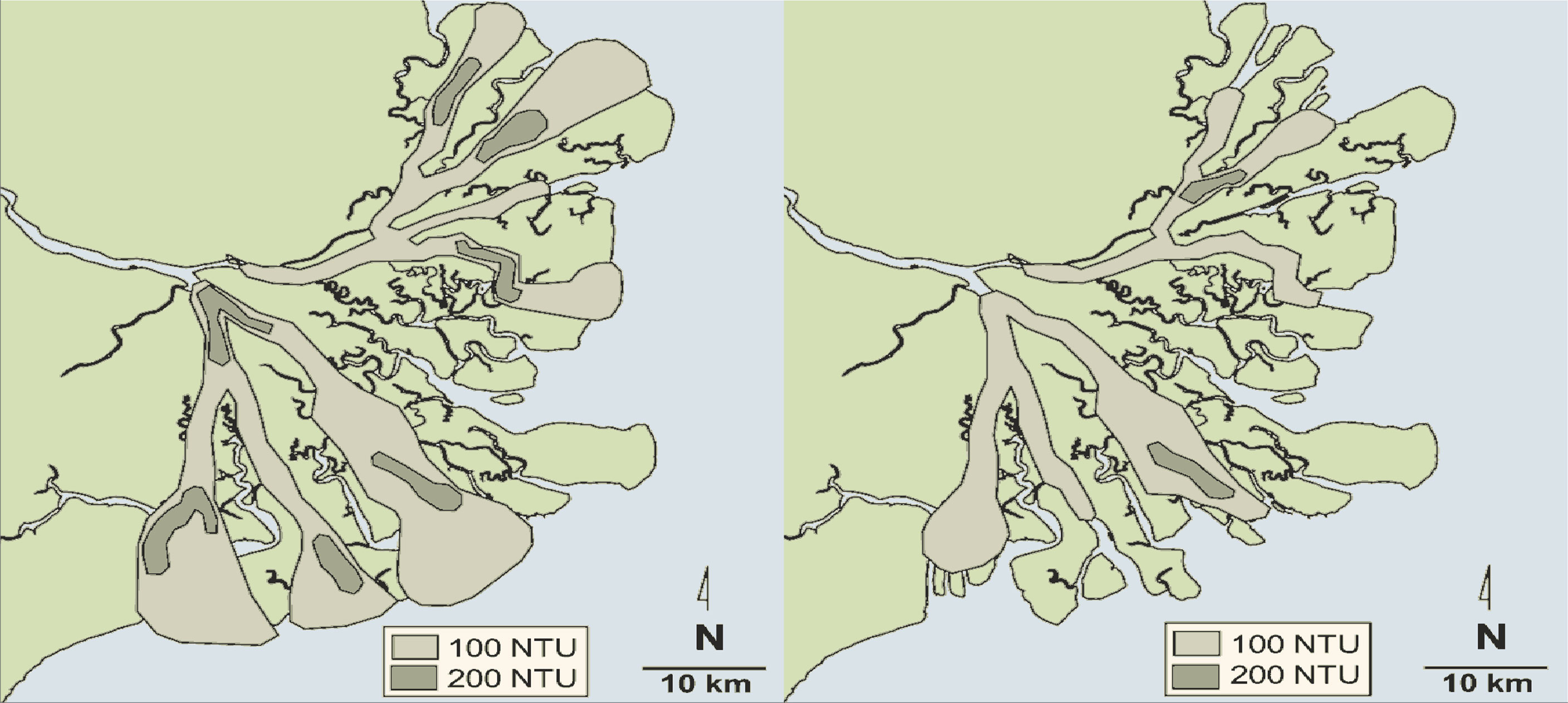
Figure 1 Bottom turbidity in nephelometric turbidity units (NTUs) of the Mahakam Estuary in Indonesia during maximum ebb at spring tide (left) and at neap tide (right), adapted from Salahuddin and Lambiase (2013).

Hence, the focus of this study is on gaining more fundamental understanding about the mechanisms that determine the ETM dynamics in estuarine channel networks. Specifically, the aim is to understand the dependence of ETMs in an estuarine network on fluvial sediment discharge and on changes in depth and width in one channel of the network. To do so, the contributions and sensitivity of various physical processes and of sediment overspill between channels will be investigated. In this study, we focus on estuaries in which the transport of sediment is mainly due to river flow and density-driven flow.

To address these aims, an idealised semi-analytical width-averaged model of an estuarine network will be developed and analysed. This choice is motivated by earlier work (see, e.g., Chernetsky et al., 2010), in which it was demonstrated that such a model allows for separating the contributions of various physical processes to the transport and accumulation zones of fine sediments in single channels. Furthermore, an idealised model is fast and flexible, which makes it suitable for extensive sensitivity analysis. The model will be applied to an idealised three-channel network (one river and two sea channels), as this is the simplest case that still describes the sediment transport mechanism acting in general estuarine networks. This choice is also motivated by several previous studies. Buschman et al. (2010) and Sassi et al. (2011) investigated the tidal and residual hydrodynamics of such a network configuration with a 3D numerical model. Iwantoro et al. (2022) used a 1D, cross-sectionally averaged model to quantify sand transport and morphodynamics in a three-channel network. Motivated by the field observations described above, we will specifically study what happens to locations and intensities of ETMs if 1) sediment discharge from river is increased, 2) depth of one of the seaward channels is varied, and 3) width convergence in one of the seaward channels is varied. Thereafter, to discuss the implications considering human intervention, robust sensitivity results will be generalised and discussed within the literature.

The model and methods of analysis are detailed in Section 2. Results are presented in Section 3, followed by a discussion (Section 4) and the conclusions (Section 5).

2. Model and methods

The model used to study the ETM dynamics is an extension of iFlow (Dijkstra et al., 2017) to a network. The iFlow model is a modular modelling framework for a systematic analysis of the width-averaged water motion and sediment transport in a tidally dominated estuarine system. Here, the geometry, water motion, and suspended sediment dynamics will be briefly described and the key aspects of the model will be stated with the matching conditions for suspended sediment. The reader is referred to the Supplementary Material for the full governing equations and boundary conditions within each channel.

2.1. Geometry and water motion

The network considered in this study is shown in Figure 2. Each channel j (where j=1,2,3) has a length L_j and is represented by a constant depth H_j. Positions in each channel are specified by Cartesian coordinate systems x_j and z_j, where x_j is the along-channel coordinate increasing from the landward boundary (x_j = 0) to the seaward boundary (x_j = L_j) and the z-axis points vertically upward from the bottom z_j = –H_j to the free water level z_j = η_j with respect to the mean sea z = 0. The depth-independent width B_j is either constant or has an exponential profile

FIGURE 2

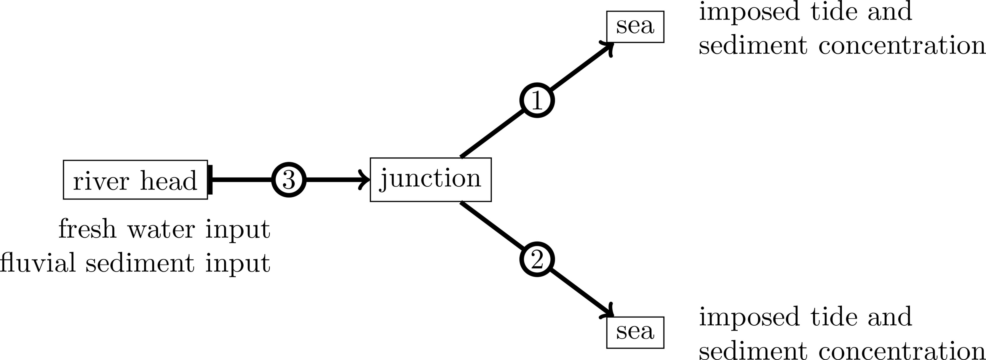
Figure 2 Sketch of the three-channel estuarine network considered in this study. Numbers in circles indicate channel numbers.

$\begin{array}{ll}B(x)=B_o\exp \frac{x-L}{L_b}& (1)\end{array}$

where B_o is the channel width at x = L, and L_b is the upstream width convergence length scale. Here and further in this text, the channel indices are omitted for legibility if the equation holds for all channels.

Neglecting the Coriolis effect and horizontal turbulent diffusion, the water motion in all channels is governed by the Reynolds- and width-averaged shallow water equations (see Supplementary Eqs. S1, S3). These determine the horizontal velocity u(x, z, t), the vertical velocity w(x, z, t), and the level of the free surface η(x, t) with respect to z = 0 in every channel, where t denotes the time. Turbulence in the model is determined by a vertical eddy viscosity A_v, which is assumed to be constant in the vertical and in time and is proportional to the mean water depth. This choice is motivated by studies of Festa and Hansen (1978); Chernetsky et al. (2010), who successfully simulated ETM dynamics in a single channel. A linear equation of state is assumed (Supplementary Eq. S2), in which the water density depends on only a prescribed tidally and depth-averaged salinity through the haline contraction coefficient β_s. Suspended sediment concentrations are assumed to be relatively low so that their effect on the density is ignored.

The water motion is externally forced by a prescribed semi-diurnal (M₂) tidal water level at every seaward boundary and a tidally averaged river discharge at the landward boundary. The water motion in different channels is connected by assuming continuity of dynamic pressure and conservation of mass (see Supplementary Eq. S5).

2.2. Suspended sediment dynamics

The modelled suspended sediment in all channels is assumed to consist of one fine sediment fraction. The sediments form flocs with a certain density, and hence, the settling velocity w_s is constant. In every channel, the width-averaged sediment mass concentration c(x, z, t) is governed by the suspended sediment mass balance (see Supplementary Eq. S6). The erosive flux at the bed is assumed to be proportional to the magnitude of the bottom stress τ_b and to the availability f (Friedrichs et al., 1998) of sediment, which is the model output. It further contains a given constant erosion parameter M̂.

The availability f measures the subtidal abundance of sediment available for erosion near the bed. In this study, only the case 0 ≤ f ≪ 1 is considered, meaning that the values of suspended sediment concentration are relatively low. The availability f(x) is determined using the morphodynamic equilibrium condition (Friedrichs et al., 1998; Chernetsky et al., 2010). Essentially, the morphodynamic equilibrium implies that the tidally averaged deposition is balanced by the tidally averaged erosion near the bed. Consequently, the net sediment transport ℱ is constant in every channel. Denoting the averaging over a tidal cycle by ⟨·⟩, it reads

$\begin{array}{ll}ℱ=\langle B{\displaystyle {\int }_{-H}^{\eta }(uc-K_h\frac{\partial c}{\partial x}})dz\rangle & (2)\end{array}$

where K_h is a constant horizontal eddy diffusivity.

A time-mean, depth-averaged sediment concentration c_sea is prescribed at the seaward boundary of each sea channel, and a tidally averaged fluvial sediment mass flux ℱ_river is imposed at the river head. Sediment concentration in different channels is matched through mass conservation of the sediment. Moreover, it is assumed that the depth-averaged subtidal concentration is continuous at each junction.

Eq. (2) results in an equation for sediment availability f, which reads

$\begin{array}{ll}ℱ=BT(x)f+BF(x)\frac{\text{d}f}{\text{d}x},& (3)\end{array}$

where the function T is referred to as the subtidal advective transport capacity per unit (p.u.) width, i.e., the advective transport p.u. width when the water column is everywhere saturated during the entire tidal cycle. It contains the most sediment transport processes such as the transport by residual current and tidal pumping. The quantity F describes dispersive sediment transport capacity p.u. width. The effect of spatial settling lag (de Swart and Zimmerman, 2009) is explicitly contained in both T and F. Assuming the sediment concentration does not influence the water motion, the transport capacity p.u. width T is fully determined by the flow conditions and independent of the actual sediment concentration.

The detailed solution methods can be found in the Supplementary Material and in Dijkstra et al. (2017). Note that the model directly solves for the equilibrium solutions (Supplementary Eqs. S18–S20), and hence, time stepping is not required.

2.3. Analysis methods

The aim of this section is to present the concepts that are used for the interpretation of the results. In this study, an ETM will be referred to as a local maximum in the depth-averaged subtidal sediment concentration $\overline{c}$, which reads

$\begin{array}{ll}\overline{c}=\frac{1}{H}\langle {\displaystyle {\int }_{-H}^{\eta }c\text{d}z}\rangle .& (4)\end{array}$

The location where availability f attains a local maximum will be referred to as the location of sediment trapping. The availability gradient $\frac{df}{dx}$ vanishes at the trapping location, and Eq. (3) reduces to ℱ = BTf, i.e., the net sediment transport equals the advective transport. Note that the gradient of transport capacity is required to be negative$(\frac{dT}{dx}<0)$ for the existence of the sediment trapping location. The subtidal carrying capacity Ĉ (kg m^-2 is the subtidal maximum amount of sediment that can be suspended in the water column for maximum erosion, i.e.,

$\begin{array}{ll}\widehat{C}=\langle {\displaystyle {\int }_{-H}^{0}c{|}_{f=1}dz}\rangle ,& (5)\end{array}$

which is a property of the flow and fully determined by local resuspension. It is a depth-integrated quantity, and hence, it scales with depth. It is shown in the Supplementary Material that the carrying capacity is fully determined by local resuspension (Supplementary Eq. S17). The depth-averaged subtidal concentration $\overline{c}$ can then be written as the product of the subtidal carrying capacity Ĉ and availability f (Supplementary Eqs. S16, S17) It follows that $\frac{\text{d}\overline{c}}{\text{d}x}=\widehat{C}\frac{\text{d}f}{\text{d}x}+f\frac{\text{d}\overline{C}}{\text{d}x}.$ Namely, the location of ETM is not the same as the location of sediment trapping, but they are close when the carrying capacity Ĉ is almost spatially uniform. Therefore, the ETM dynamics will be analysed using the carrying capacity Ĉ and availability f. Here, it will be briefly described how the changes in Ĉ and f can be explained. As the sediment is resuspended by the tidal current, any change in carrying capacity can be understood by considering the changes in tidal current amplitudes. The availability f carries the information of horizontal processes, as it results from the net sediment transport ℱ and transport capacity p.u. width T. The changes in the availability will be explained in terms of the net sediment transport ℱ and transport capacity p.u. width T.

As ETMs often coincide with sediment trapping locations, the effects of changing net sediment transport ℱ and advective transport BTf on sediment trapping location are conceptualised in Figure 3. The intersection ① of ℱ₁ and (BTf)₁ is the location of sediment trapping (subscript is the channel index). A reduced net sediment transport ℱ₂ causes the location of sediment trapping to move seaward to the location of crossing ②. Keeping the net sediment transport ℱ₁ fixed, a reduced advective transport (BTf)₂ leads to the sediment trapping location shifting landward to the location of crossing ③. The combination of the two changes leads to the trapping location crossing ① travelling to crossing ④. Depending on the gradient of the advective transport, the sediment trapping location may move in either direction with respect to the location of crossing ①. In Figure 3, it moves slightly landward.

FIGURE 3

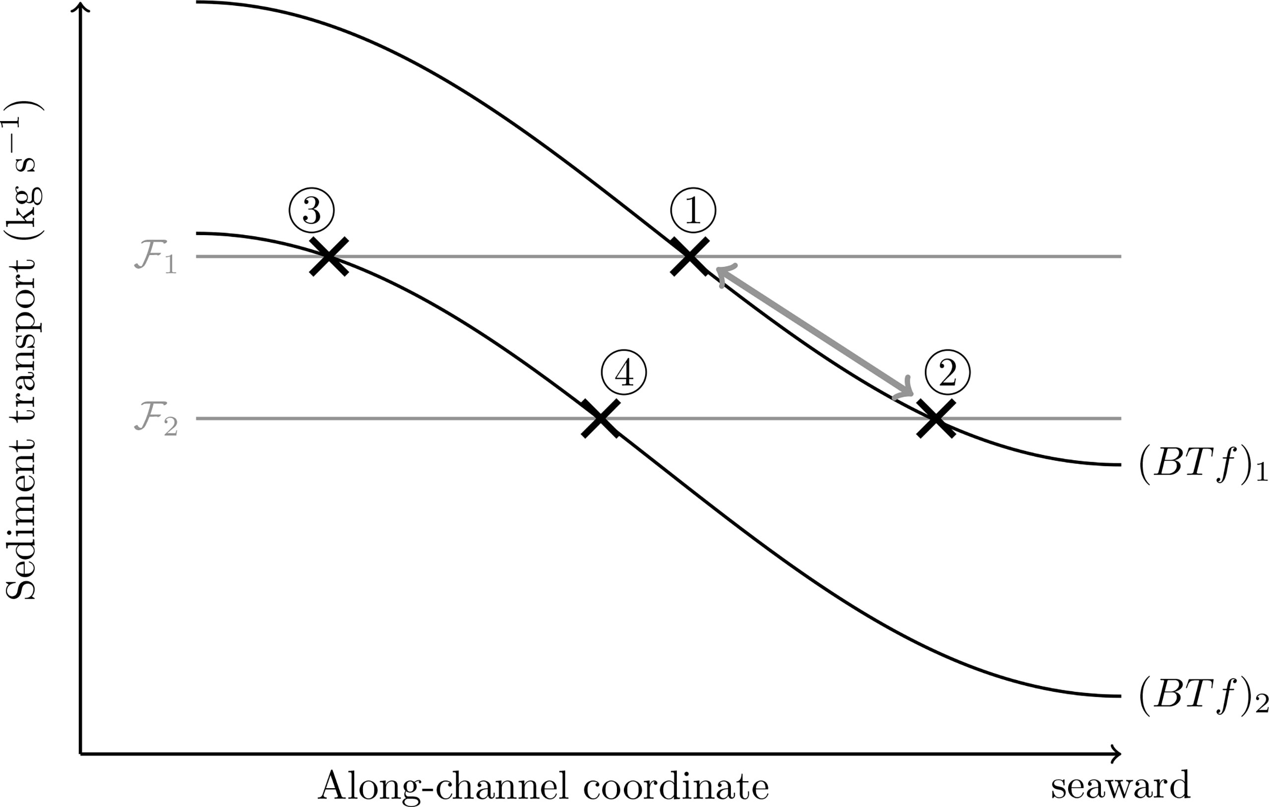
Figure 3 A conceptual figure showing the effects of changing net sediment transport ℱ (grey) and advective transport BTf (black) on the location of sediment trapping (cross), assuming small influence of net sediment transport on the availability.

Following the definition for salt water overspill (Wu et al., 2006), sediment overspill is observed in a channel if the net sediment transport ℱ is negative (landward) in that channel.

2.4. Design of model experiments

The default parameter values for the reference case of the idealised three-channel system (Figure 2) are contained in Table 1. These values are representative for a coastal plain estuarine network. Channel 3 is made sufficiently long (1,000 km), such that the tidal influence vanishes at the tidal limit. The area of interest in Channel 3 is the most seaward 40 km. The water motion is forced by a constant river discharge Ǫ_river = 1,000 m³ s^-1(positive value indicates seaward) from the landward boundary of Channel 3 and M₂ water level amplitude of 1 m at the seaward boundary of both Channels 1 and 2. A subtidal depth-averaged sediment concentration c_sea = 0.05 m⁻³ is prescribed at the seaward boundary of Channels 1 and 2 and the fluvial sediment input is ℱ_river = 50 kg s⁻¹, imposed at the river head. The prescribed salinity profile and its gradient are shown in Figure 4. Note that the three channels share the same along-channel coordinate, where x=0 is the junction. Using the morphodynamic equilibrium, the modelled suspended sediment concentration is insensitive to the erosion parameter (Supplementary Eq. S8), which only has influence on the magnitude of the availability and hence the net sediment transport.

FIGURE 4

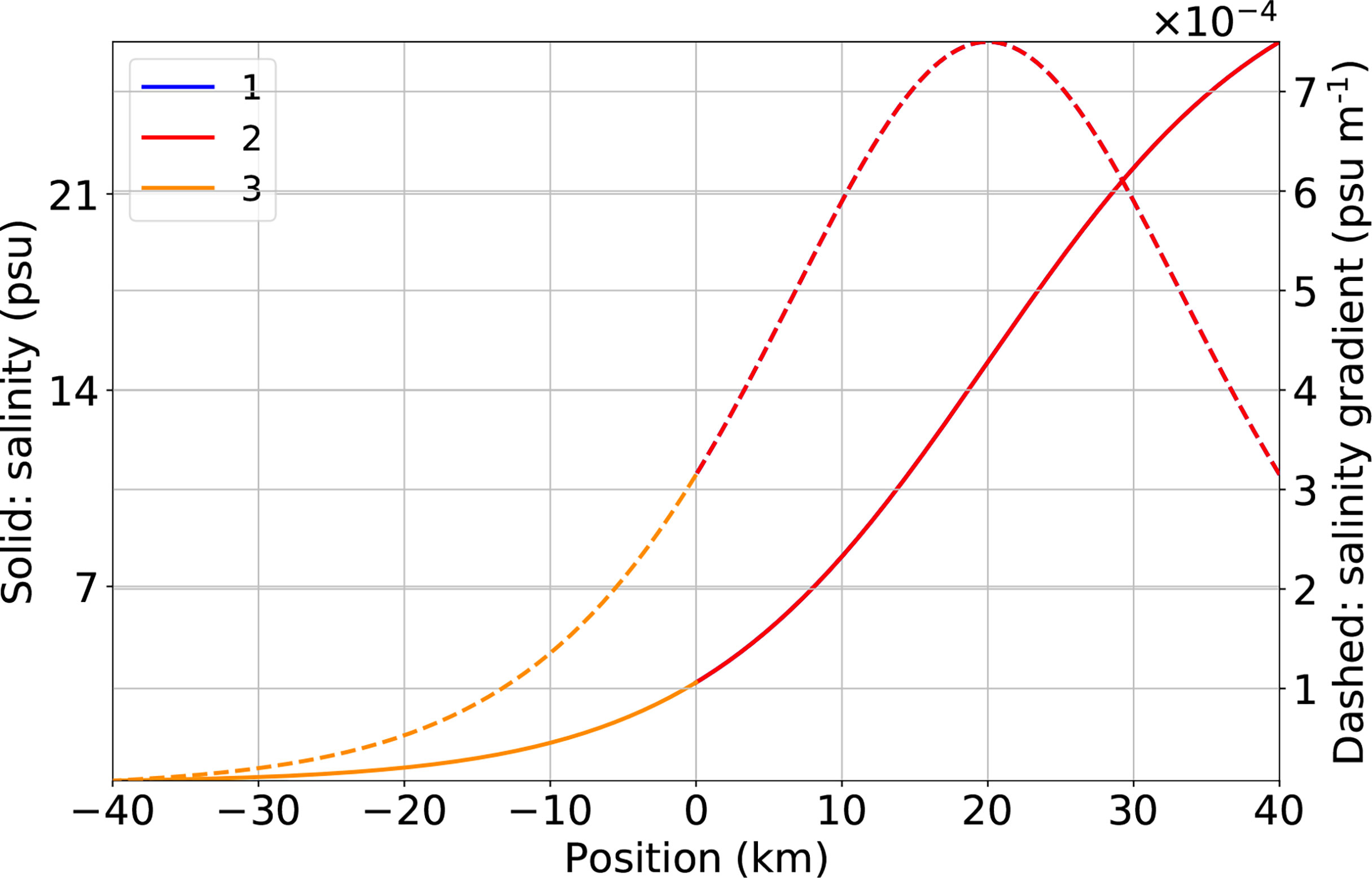
Figure 4 The salinity (solid line) and its gradient magnitude (dashed line) for all experiments.

TABLE 1

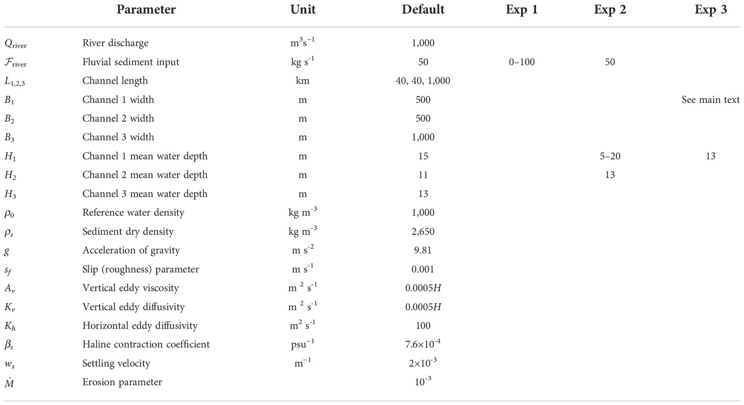
Table 1 Parameter values (representative for a coastal plain estuarine network).

In order to address the specific aims, three sets of experiment will be conducted to show the sensitivity of the ETM dynamics to different parameters. First, the fluvial sediment input is varied from 0 to 100 kg s^-1 whilst keeping the fresh water discharge fixed. This is equivalent to varying an imposed sediment concentration at the landward boundary. Second, the fluvial sediment input is reset to 50 kg s⁻¹, the mean water depth in all channels is set to 13 m, and the mean water depth in Channel 1 is varied from 5 to 20 m. Third, the depth of Channel 1 is set to 13 m, and its width at the sea is varied from 500 to 2, 000 m, with its width at the junction fixed at 500 m, i.e., increasing width divergence. Its width profile follows Eq. (1).

3. Results

3.1. Reference case

The spatial structure of the subtidal concentration is determined by the current, the characteristics of which are shown in Figure 5. The width and depth-averaged M₂ tidal current amplitudes (Figure 5A, solid) are approximately 0.8 ms^-1 and slightly decrease upstream. It is one order of magnitude larger than that of the internally generated M₄ overtide (dashed line), which increases upstream. The phase of the M₂ tidal current decreases upstream in all channels, from which it follows an almost spatially uniform upstream phase velocity of 10 ms^-1 (Supplementary Figure S1). The internally generated overtides (M₄) are phase locked to the forcing tide (M₂). The phase speed of the M₄ current is also about 10 ms^-1. The residual current is seaward everywhere at the surface (dashed line) and is landward near the bottom (solid line) in Channel 1 for x between 10 and 30 km (Figure 5B). This is due to the density-driven exchange flow (imposed salinity field), as follows from Supplementary Figure S2, which shows all components in the residual flow. Recall that the salinity profile in all channels is shown in Figure 4. The depth-averaged residual current (dotted line) is seaward in all channels due to the prescribed river discharge. In Channel 3, it is slightly larger than the river flow velocity ($\frac{Q_{river}}{B_3{H}_3}$). This is because the latter is a mass transport velocity, which also accounts for Stokes transport by the tidal wave. This difference vanishes at the river head where the river discharge is imposed. The depth-averaged residual current is much larger in Channel 2 than that in Channel 1.

FIGURE 5

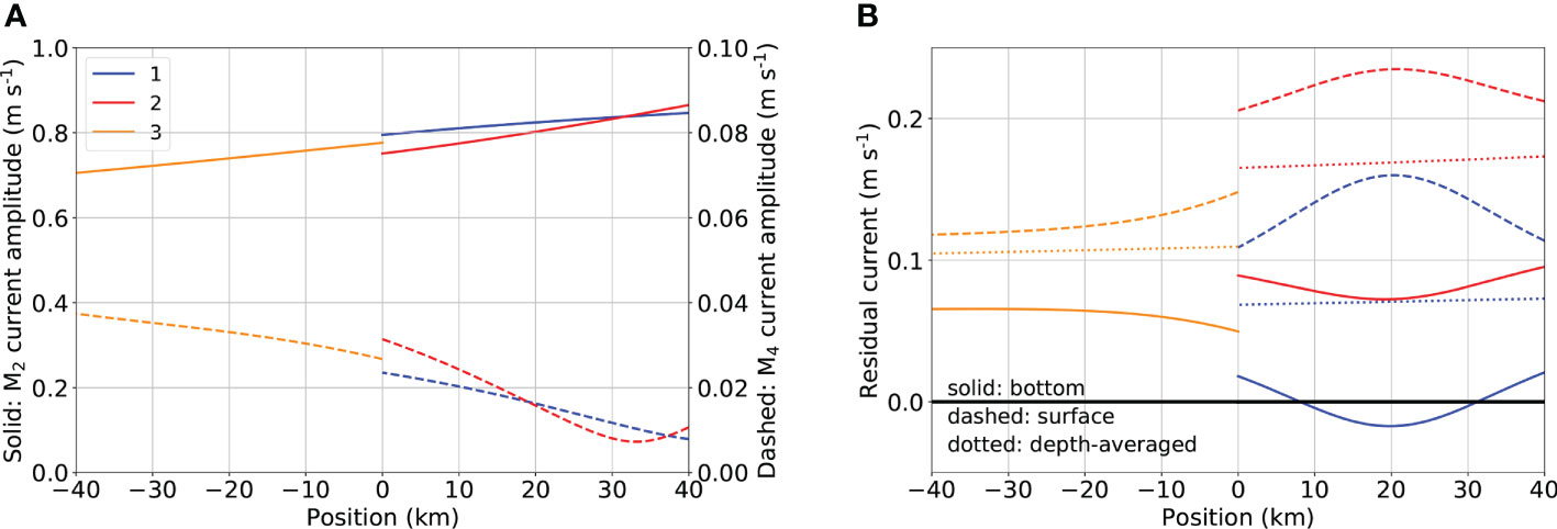
Figure 5 Tidal and subtidal currents for the reference case. (A) Depth-averaged M₂ (solid lines) and M₄ (dashed lines) current amplitudes. (B) Residual currents on the bottom (solid lines), near the surface (dashed lines), and depth averaged (dotted lines).

The subtidal suspended sediment concentration in all three channels for the reference case is shown in Figure 6A, with the depth-averaged values contained in Figure 6B. Two ETMs can be observed. One is near x=10 km in Channel 1 and the other is near x=15 km in Channel 2. The along-channel structure of the concentration is mainly controlled by the structure of the availability f (Figure 6C, solid line). In every channel, the carrying capacity $\widehat{C}$ (Eq. 5) follows the M₂ current amplitude, and it increases downstream (Figure 6C, dashed line), 10⁻⁵ kg m⁻³. This results in a small shift of the locations of the ETM towards the sea with respect to the locations of the sediment trapping (maximum in f ).

FIGURE 6

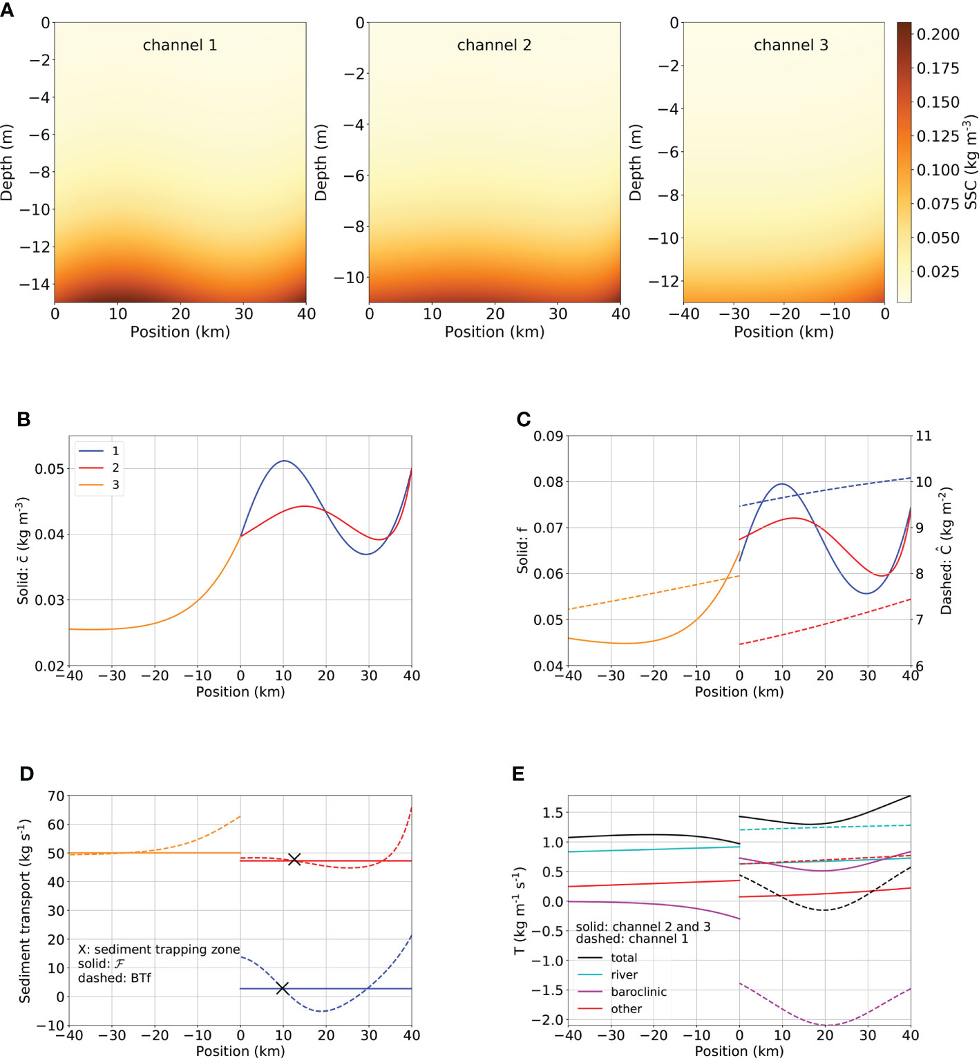
Figure 6 Results for the reference case. (A) Subtidal suspended sediment concentration (SSC) in the three channels. (B) The subtidal depth-averaged SSC $\overline{c}$. (C) Availability f (solid lines) and carrying capacity $\widehat{C}$ (dashed lines). (D) The net sediment transport ℱ (solid lines) and the advective transport BTf (dashed lines). (E) Difference contributions to T, the transport capacity per unit of width.

Figure 6D shows the net sediment transport ℱ (solid line) together with the advective transport BTf (dashed line). Each of the downward intersections of the net sediment transport ℱ and advective transport BTf corresponds to a sediment trapping location and is indicated by a cross, confirming the two sediment trapping locations near x=10−15 km. The net sediment transports in Channels 1 and 2 are 3 kg s⁻¹ and 47 kg s⁻¹, respectively, with the sum the same as the imposed net sediment transport in Channel 3 (ℱ₃=50 kg s⁻¹). Sediment overspill is not observed in the reference case.

In Figure 6E, along-channel profiles of the total transport capacity per unit width T are shown (black lines), and its various components. In this particular setting, the most dominant contributions to T are the residual transports by density-driven flow (baroclinic, magenta) and river flow (cyan). The solution for density-driven flow in a single-channel estuary is given in Geyer and MacCready (2014) and references therein, and Wang et al. (2022) presents the solution for a channel network. The density-driven flow imports sediment from the sea in Channel 1 and exports sediment into the sea through Channel 2. The river flow flushes sediment seaward in all channels. All other contributions to T, such as the transport of sediment by tidally rectified currents, tidal pumping, sediment dispersion, and spatial settling lag, are summed in “other” (red).

3.2. Fluvial sediment input

The sensitivity of the net sediment transport in Channels 1 and 2 to the prescribed fluvial sediment input is illustrated in Figure 7. There is net exchange of sediment from Channel 1 to 2 of 5 kg s⁻¹. This is best seen in Figure 7 in which the fluvial sediment input is 0, where the net sediment transports in Channels 1 and 2 are equal in magnitude but have opposite directions. Additionally, the net sediment transport in both Channels 1 and 2 are linear in the prescribed fluvial sediment input, meaning that a fixed fraction of the fluvial sediment is allocated into each channel. This is explained in Section 3 of the Supplementary Material.

FIGURE 7

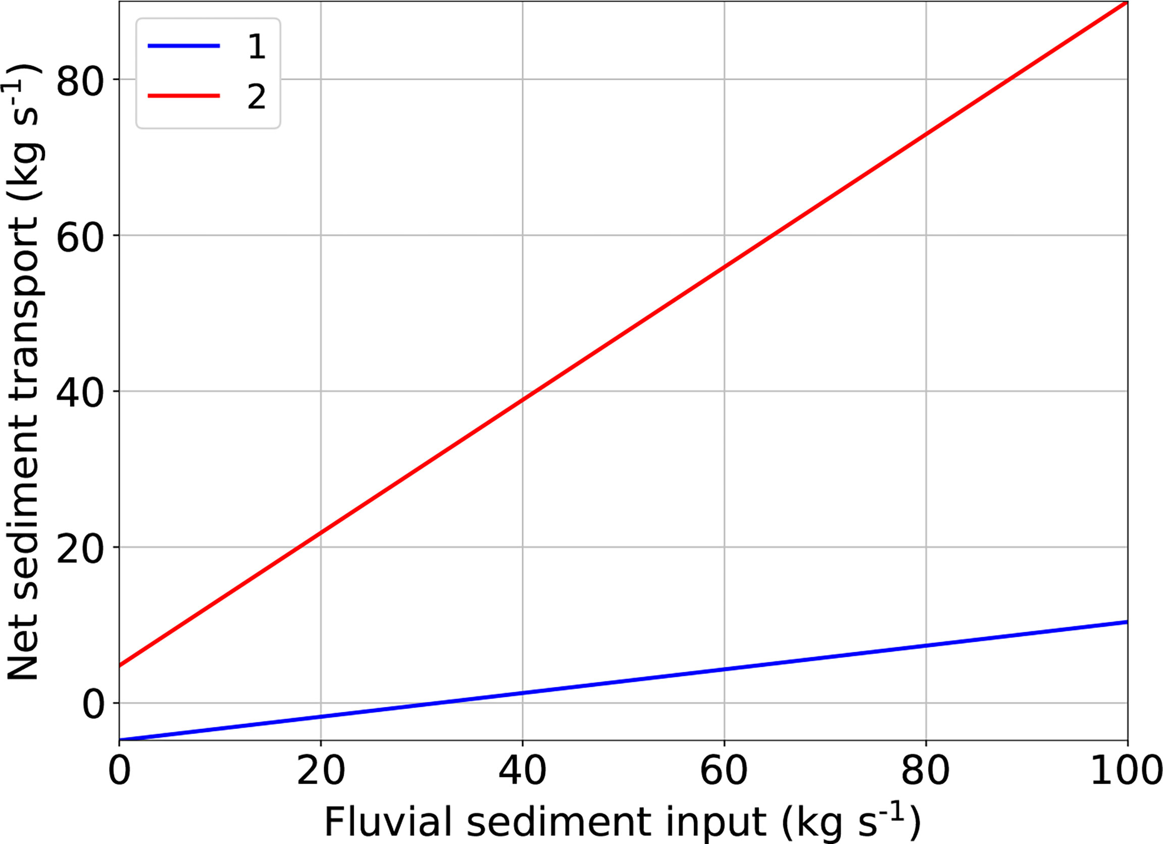
Figure 7 Sensitivity of net sediment transport in Channels 1 and 2 to fluvial sediment input.

The sensitivity of ETMs in the system to fluvial sediment input is summarised in Figure 8. The black curves in the plots containing the depth-averaged subtidal concentration $\overline{c}$ (top row) and availability f (bottom row) indicate the location of ETM and zone of sediment trapping, respectively. The black curve is obtained by connecting the positions of the local maxima in the associated plotted quantity for every value of fluvial sediment input. As fluvial sediment input increases, availability f rises in all channels, which in turn leads to the increase in sediment concentration $\overline{c}$. Changing fluvial sediment input has no influence on the carrying capacity $$\widehat{C}$$ and transport capacity p.u. width T. To analyse the locations of trapping and the associated ETMs, the framework illustrated earlier in Figure 3 is used. With increasing fluvial sediment input, the net sediment transports in both channels increase faster than the advective transport BTf so that the intersections between advective transport capacity BTf and net sediment transport ℱ, which indicate the locations of sediment trapping, move upstream. Furthermore, the upstream shift of the location of sediment trapping in Channel 2 is much weaker than that in Channel 1, albeit Channel 2 receives more sediment from the upstream channel. This is because the magnitude of availability in Channel 2 increases faster than that of Channel 1 locally near the ETM location (Figure 3).

FIGURE 8

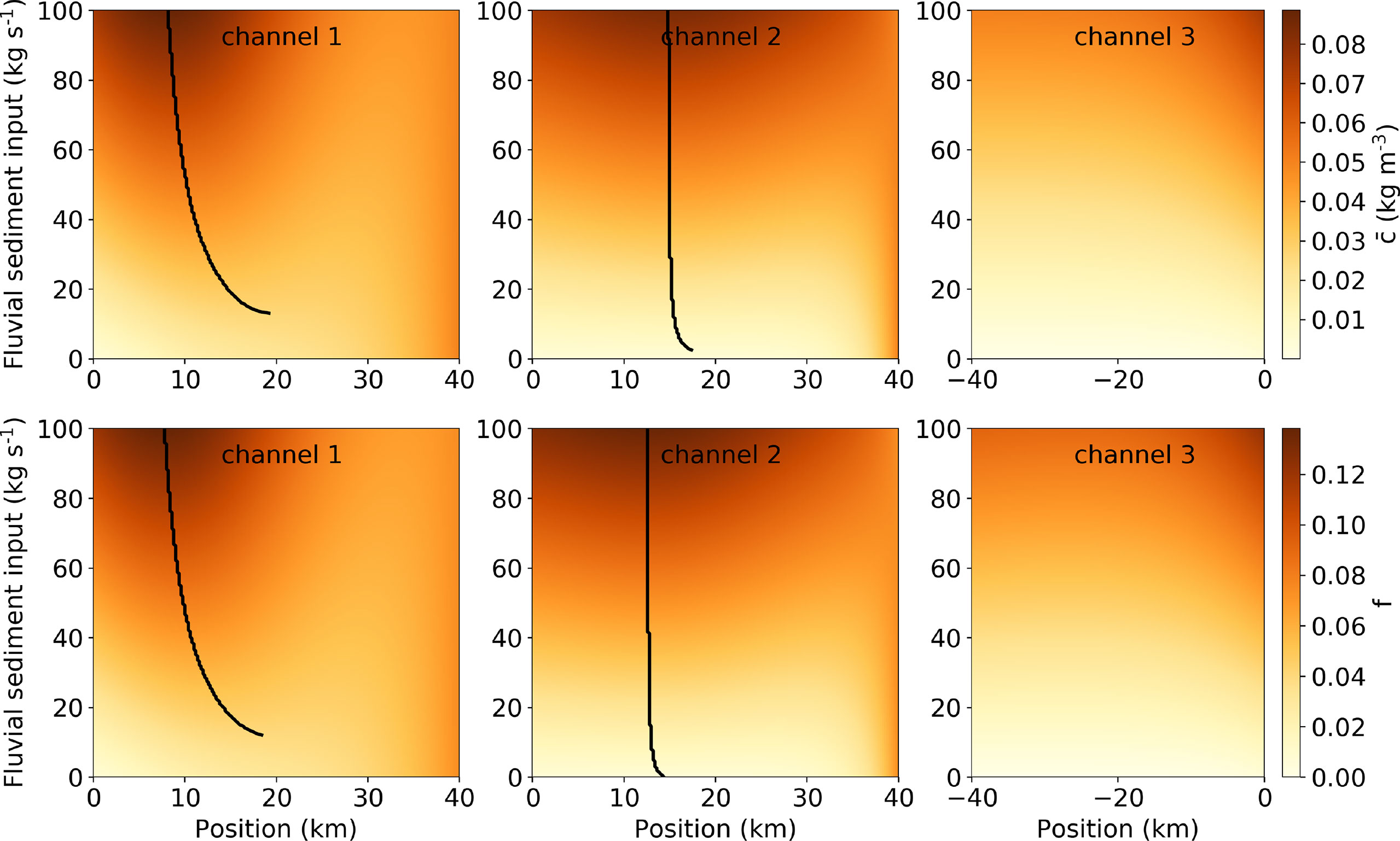
Figure 8 Sensitivity of along-channel distributions of depth-averaged subtidal concentration (first row) and availability (second row) to fluvial sediment input. Black curves indicate the location of local maxima.

3.3 Local deepening

In this experiment, the depths of both Channels 2 and 3 are 13 m, whilst the depth of Channel 1 varied. Figure 9 shows the sensitivity of net sediment transport in both Channels 1 and 2 to the mean water depth of Channel 1 H₁. When H₁ is also 13 m, Channels 1 and 2 are identical. In that case, the fluvial sediment input is equally distributed into Channels 1 and 2. Net sediment transport in Channel 1 is larger than that in Channel 2 when H₁ is between 7.8 and 13m. Sediment overspill is observed in Channel 1 for H₁ larger than 15.4 m.

FIGURE 9

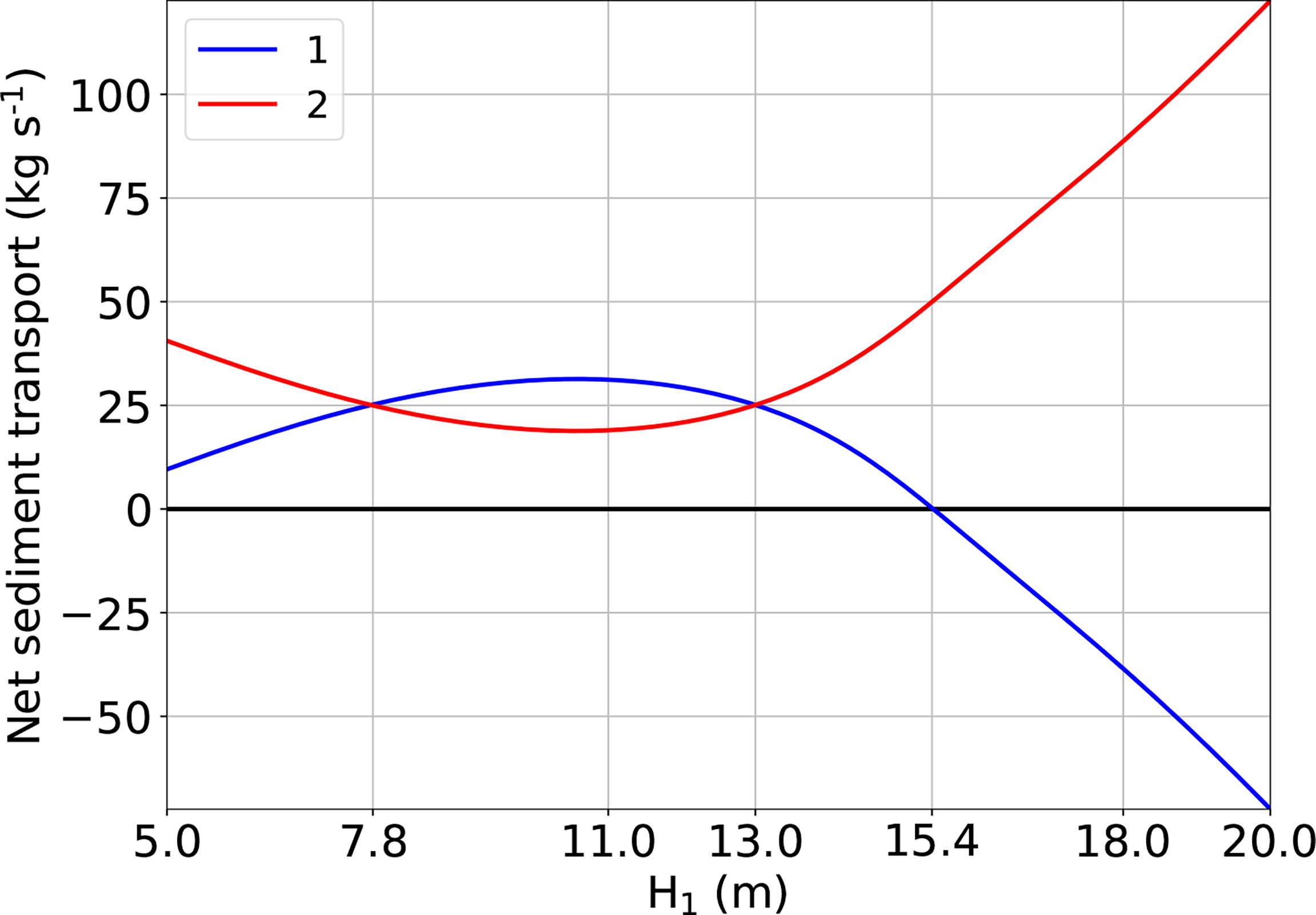
Figure 9 Sensitivity of net sediment transport in Channels 1 and 2 to the mean water depth of Channel 1.

To analyse and understand the dependence of the ETM location on the local deepening of Channel 1, the sensitivities of along-channel distributions of depth-averaged subtidal concentration $\overline{c}$ (first row), carrying capacity $$\widehat{C}$$ (second row), availability f (third row), and transport capacity p.u. width T (fourth row) to Channel 1 mean water depth H₁ are presented in Figure 10. For H₁ = 5 m, there is an ETM in Channels 2 and 3 (first row). As H₁ increases, the ETM in Channel 2 occurs slightly more upstream, and that in Channel 3 occurs more downstream towards the junction and eventually (for H₁=11 m) disappears. A third ETM appears in the system in Channel 1 when its depth reaches about 7 m and shifts rapidly downstream for increasing depth. For H₁>11 m, the shift of the ETMs in both Channels 1 and 2 changes direction. The concentration in the ETM in Channel 2 gradually increases with the depth of Channel 1, whereas the intensity of the ETM in Channel 1 attains a maximum when H₁≈16 m. The concentration at the sea (x=40 km) in both Channels 1 and 2 is unaffected by the depth of Channel 1 due to the imposed boundary condition.

The carrying capacity $\widehat{C}$(second row) in each channel changes with little along-channel variation to the depth of Channel 1 H₁ . Recall that the carrying capacity is the depth-integrated and tidally averaged suspended sediment concentration if there is always sediment available for erosion on the bed, which is a function of the along-channel coordinate. The parameter along the vertical axis in this plot is the mean water depth of Channel 1, which has been varied from 5 to 20 m. Hence, the carrying capacity is larger in Channel 1 if the mean water depth in Channel 1 is larger. In Channels 2 and 3, the changes in the carrying capacity are due to the changing erosion strength caused by the M₂ tidal current amplitudes. Since the carrying capacity scales with depth (Eq. 5), the changes in $\widehat{C}$ of Channel 1 characterise the along-channel uniform effect of increasing depth. As the depth of Channel 1 increases from 5 to 20 m, the relative changes in carrying capacity are 250% , −44% , and 22% in Channels 1, 2, and 3, respectively. The carrying capacity in Channel 2 decreases as the depth of Channel 1 increases because of the reduction in the M₂ tidal current amplitudes in Channel 2.

The dependence of availability f (third row) on the mean water depth of Channel 1 H₁ in every channel is qualitatively the same as that of the concentration in the first row of Figure 10 because the carrying capacity is fairly uniform in along-channel direction (Eq. 5).

FIGURE 10

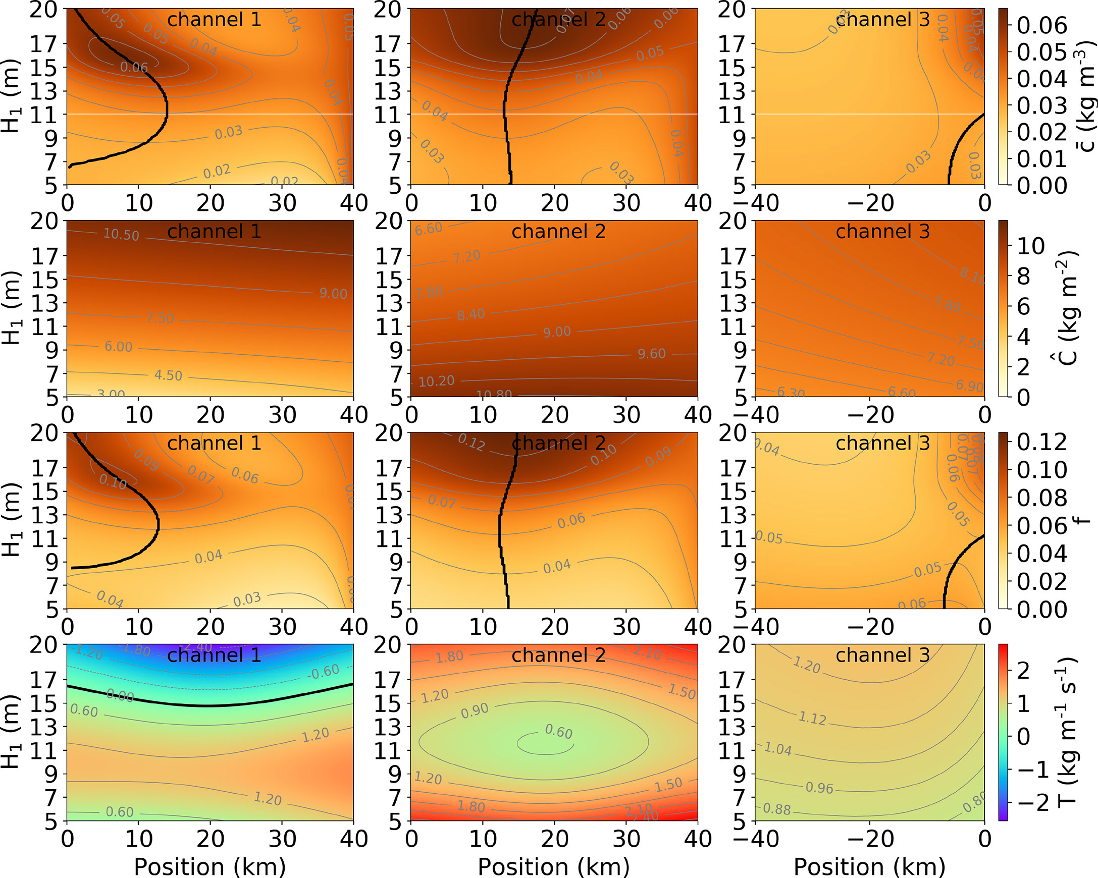
Figure 10 Sensitivity of along-channel profiles of depth-averaged subtidal concentration (first row), carrying capacity (second row), availability (third row), and transport capacity p.u. width (fourth row) to the mean water depth of Channel 1. The white line in the first row is where H₁ = 11 m.

To further understand the response of the location of maximum availability f to increasing H₁, the advective sediment transport capacity p.u. width T (fourth row) is now analysed. The black contour in the plots for the T is the 0 level. For increasing depth of Channel 1 H₁, the changes in T in Channels 1 and 2 are on averaged opposite. This is because of the net sediment transport associated with the net water transport. Since the sum of the net water transports in Channels 1 and 2 is the prescribed river discharge, an increase in the net water transport in one of the channels implies a decrease in the net water transport in the other. Consequently, the advective transport capacities in Channels 1 and 2 respond oppositely to increasing H₁.

The different responses of the ETM locations for H₁ smaller and larger than 11m in both Channels 1 and 2 can be understood as follows. For increasing H₁, the depth of Channel 2 remains 13m. Hence, the sediment transport in Channel 2 is only influenced by the changing net water transport, primarily due to river flow and density-driven flow. The net water transport due to river flow scales with depth, whilst the net water transport due to density-driven flow scales with depth squared (Wang et al., 2022). For a relatively small depth of Channel 1 (H₁<11 m), the river flow contribution to the sediment transport capacity T in Channel 2 is more important than the density-driven flow contribution (Supplementary Figure S3A). The increasing H₁ therefore leads to weaker river flow and less seaward net sediment transport in Channel 2. The sediment transport capacity in Channel 2 decreases more rapidly than the net sediment transport, causing the upstream shift of the ETM in Channel 2 (Figure 3). For a relatively large depth of Channel 1 (H₁>11 m), the density-driven flow contribution to the sediment transport capacity T in Channel 2 is more important. Hence, a larger H₁ enhances the seaward net water and sediment transports due to density-driven flow in Channel 2 that leads to the ETM in Channel 2 occurs further seaward. As increasing H₁ has opposite effects on the sediment transport due to river flow and density-driven flow, the response of the ETM in Channel 1 is opposite to that in Channel 2. The shift of the ETM in Channel 1 is larger in magnitude than that in Channel 2. This is because the exchange flow pattern in Channel 1 is intensified by its increasing depth, which is the only difference between the two channels in terms of the residual flow contribution to the sediment transport.

3.4. Channel widening

In this experiment, the mean water depth is 13 m in all channels. When the width of Channel 1 B₁ at the sea is 500 m, Channels 1 and 2 are geometrically the same, with net sediment transport being equally distributed over the two channels (Figure 11). As B₁ at the mouth increases (i.e., width divergence of Channel 1 increases), more river discharge is allocated to Channel 1. Therefore, the river current increases in Channel 1 and decreases in Channel 2, which directly causes the net sediment transport to increase in Channel 1 and to decrease in Channel 2 by river flushing. When B₁ at the sea reaches 2 km, the density-driven flow contribution to sediment transport is still dominant in Channel 2. In Channel 1, however, river and other contributions exceed that of the density-driven flow near the junction (Supplementary Figure S4). Sediment overspill is observed in Channel 2 for B₁ at the mouth larger than 1.75 km.

FIGURE 11

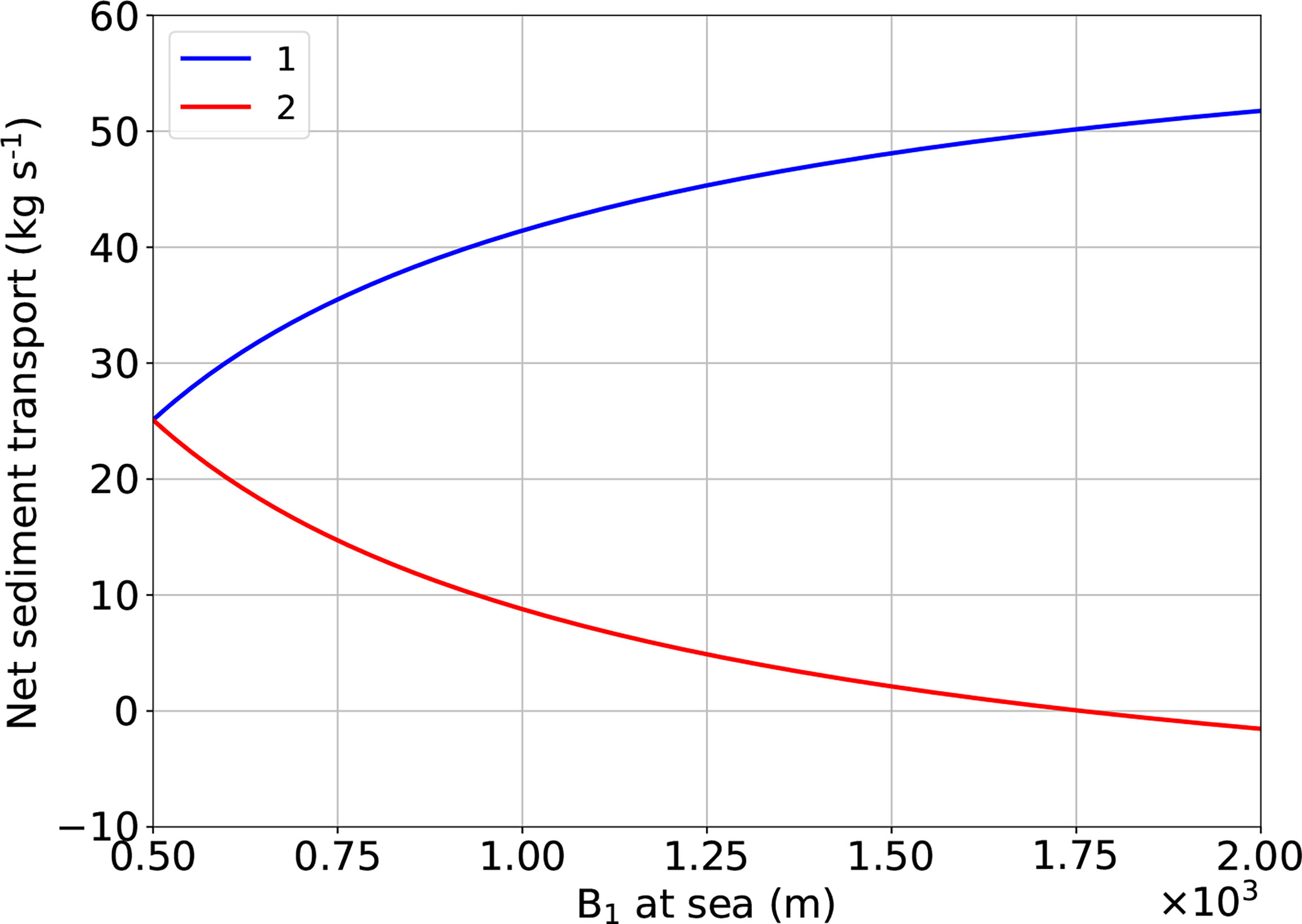
Figure 11 Sensitivity of net sediment transport to the width of Channel 1 at sea.

The sensitivity of the ETM dynamics to the width divergence of Channel 1 is summarised in Figure 12. As the width of Channel 1 B₁ increases from 5 to 20 km, the ETM in Channel 1 is observed gradually further downstream, and it intensifies by a factor of up to 2 (first row). In Channel 2, the ETM occurs slightly more upstream, and the concentration increases from 0.04 to 0.065 kg m⁻³ at the ETM. No ETM is observed in Channel 3, where the concentration is nearly unaffected by the width divergence of Channel 1.

FIGURE 12

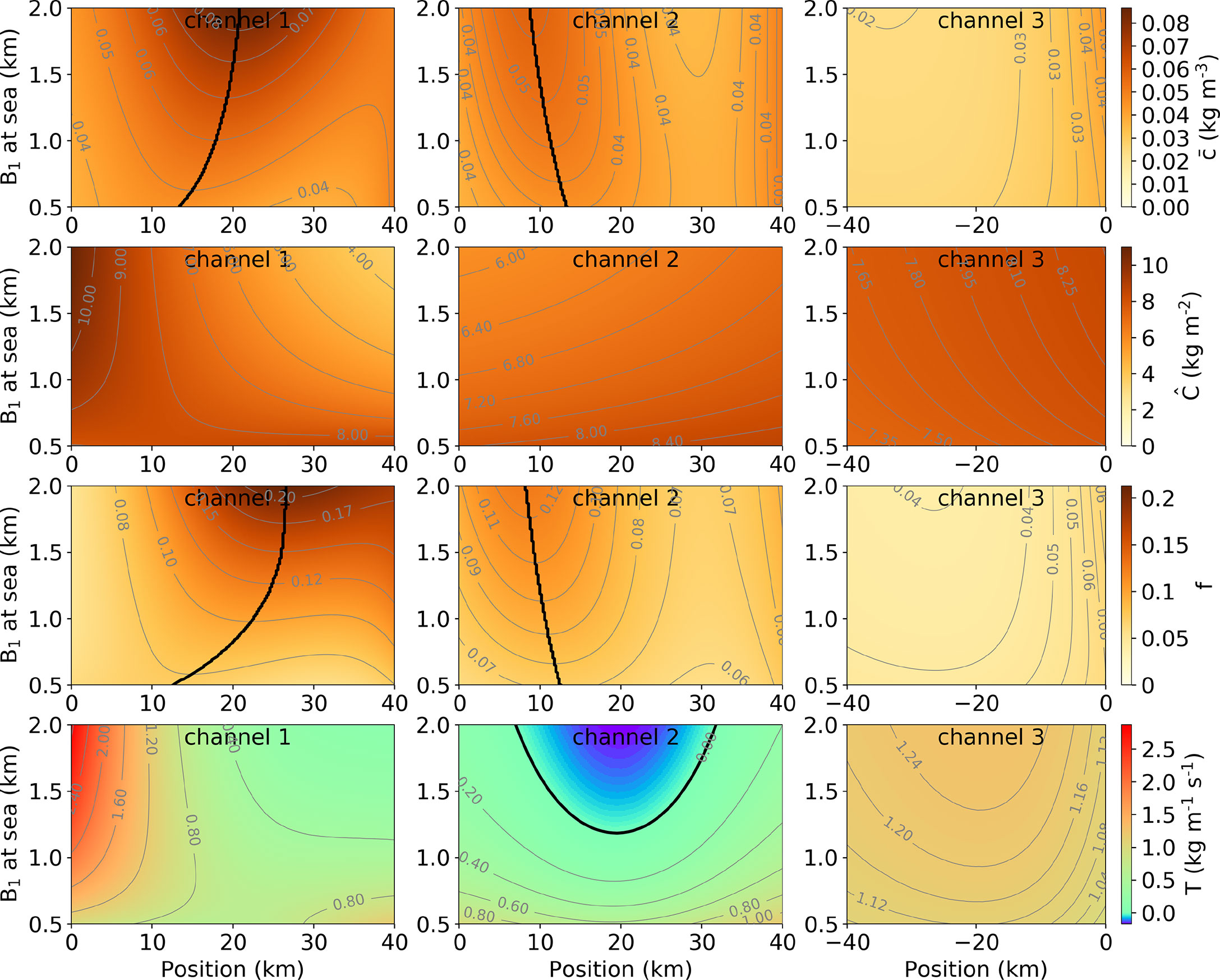
Figure 12 Sensitivity of along-channel distribution of depth-averaged subtidal concentration (first row), transport capacity p.u. width (second row), availability (third row), and carrying capacity (fourth row) to the width of Channel 1 at the sea.

The changes in the carrying capacity $\widehat{C}$ in all channels are due to the changes in the tidal current amplitudes (second row). In Channel 1, the carrying capacity ${\widehat{C}}_1$ hardly changes near the junction, whilst a noticeable reduction can be observed near the sea. This is because the tidal current in Channel 1 near the junction is constrained by that in Channel 2, the upstream tidal amplification due to stronger upstream width convergence in Channel 1 results in the reduction in the tidal current downstream. Consequently, the erosion in Channel 1 are decreasing downstream for stronger upstream width convergence, which is reflected in the carrying capacity ${\widehat{C}}_1$. There is an almost uniform decrease in the carrying capacity along Channel 2. In Channel 3, little change in the carrying capacity can be observed.

The availability f in all channels again responds in a qualitatively similar manner as the concentration to increasing width of Channel 1 at the sea (third row). However, the downstream shift of the location of sediment trapping is much stronger than that of the ETM in Channel 1 as the consequence of the decreasing gradient in the carrying capacity ${\widehat{C}}_1$. This is because the width variation in Channel 1 leads the tidal currents to vary within the channel, and hence, the carrying capacity is less spatial uniform, causing the location of ETM to differ from the location of sediment trapping.

Although B₁ at the sea is being increased, the transport capacity p.u. width T in Channel 1 hardly changes near the sea, whilst it significantly increases near the junction (fourth row). In Channel 2, the transport capacity p.u. width T₂ decreases with increasing B₁ at the sea.

As the density-driven flow is hardly affected by the channel width (Supplementary Figure S4), the ETM dynamics is mostly due to the changing distribution of the river discharge. With the widening of Channel 1, the river discharge in Channel 1 increases but decreases in Channel 2. This directly causes the ETM shifts downstream in Channel 1 and upstream in Channel 2. In Channel 1, the enhanced tidal amplifications due to stronger upstream width convergence leads to a higher resuspension rate near the junction, which alleviates the downstream shift of the ETM with respect to the sediment trapping location.

4. Discussion

The goal of this study is to gain more insight into the sensitivity of ETMs and the methods for analysing the ETM dynamics in an estuarine network. This study presents a first step, by choosing a simple network geometry and selecting model parameters such that the river flow and density-driven flow are the dominant drivers (i.e., gravitational circulation) for ETM formation. This means that results can be qualitatively related to channel network estuaries where gravitational circulation is also important, including the Yangtze (Pu et al., 2016) and Amazon (Geyer, 1993) during the dry season.

Below, these results will be placed into a broader context, and ETM responses will be compared with those reported in the literature.

The influence of settling velocity on results is weak (Supplementary Figure S5), which is consistent with that of Festa and Hansen (1978).

4.1. Fluvial sediment input

In this study, the fluvial sediment input is the imposed net sediment transport at the river head. Figure 7 shows that the net sediment transport in any channel downstream of a junction is proportional to fluvial sediment input (see also Supplementary Eq. S1). One of the key findings is that, for an ETM near the maximum availability in a channel of an estuarine network, a larger seaward net sediment transport leads to the upstream shift of this ETM and vice versa (Figure 3). This implication is not restricted to the sediment trapping caused by river flow and density-driven flow but applies in general as long as the concentration does not significantly alter the water motion. These findings are similar as the theoretical results found by Festa and Hansen (1978) using a subtidal model of a single channel. This study shows that this conclusion can be extended to the behaviour of ETMs in a network.

It has been observed in several estuarine networks that a reduced fluvial sediment input causes a downstream shift of ETMs. The construction of the Three Gorges Dam in the Yangtze River substantially reduced the fluvial sediment input into the Yangtze Estuary, with the river discharge almost unaffected, which causes the reduction in seaward net sediment transport in all distributary channels (Luo et al., 2022). By analysing in situ field measurements, combined with the Landsat images from 1979 to 2008 in the Yangtze Estuary, Jiang et al. (2013) reported that lower fluvial sediment input caused ETMs to shift seaward. The Pearl Estuary has also experienced the reduction in the fluvial sediment input due to upstream damming over the last two decades. Zhan et al. (2019) studied the inter-annual variability of the suspended sediment concentration in the Pearl Estuary from 2002 to 2014, when the yearly averaged river discharge was constant, but the fluvial sediment supply decreased. A clear seaward shift of the upstream boundary of the high concentration region was observed. Furthermore, due to the reduced fluvial sediment input in both the Yangtze Estuary and the Pearl Estuary, an overall decline in the sediment concentration was observed (Zhan et al., 2019; Luo et al., 2022), which is also captured by our sensitivity results (Figure 8).

4.2. Local deepening and narrowing

Both deepening and narrowing in one channel may affect ETMs in multiple channels (Figures 10, 12). The local change in the channel geometry affects the net sediment transport and transport capacity, and the shift of the ETMs depends on the specifics of these changes.

Using a subtidal model that accounts for the influence of sediment concentration on water density, Talke et al. (2009) showed that an ETM shifts upstream with increasing depth in a single channel with a fixed river discharge. A larger water depth causes a more intensified exchange flow pattern due to the salinity-induced density-driven flow, leading to the upstream shift of the ETM. In a network, however, the response of the location of an ETM to the deepening is more complex (Figure 10). The essential difference is that the river discharge is fixed at the river head in the upstream channel but not in the channels that are located seaward of the junction. Hence, instead of the river discharge, one needs to consider the net water transport in each channel. Focusing on the river and density-driven flow, the actual response of the ETM location to the deepening of a channel depends on which process is the dominant contribution to the net water transport, as explained in Section 3.3. Hence, deepening may cause either an upstream or downstream shift of the ETM.

Similarly, keeping the river discharge fixed, the decrease in upstream width convergence (narrowing) in a single channel enhances the river current that tends to shift the ETM downstream. The North Channel of the Yangtze Estuary experienced narrowing and reduction in width convergence as the consequence of a land reclamation project. The ETM indeed shifts downstream, as reported by Teng et al. (2021). To explain this, by careful analysis of remote sensing date in the North Channel under various flow conditions, a conceptual model is proposed to argue that the seaward shift is partly due to the enhanced ebb-dominance that causes a seaward shift of the convergence in sediment transport. Also in the Yangtze Estuary, the first stage of the Deep Waterway Project (DWP) involved only the construction of the training walls in the North Passage (NP), i.e., narrowing and reducing upstream width convergence. However, Jiang et al. (2012) reported that the ETM in the NP slightly shifts upstream after the first stage of the DWP. The reason is, in a network, the weaker width convergence locally in a channel also decreases the net water transport distributed into this channel, causing less seaward sediment flushing by the net water flow (Figure 11).

4.3. Model limitations

It should be noted that the model is exploratory (Murray, 2003) and is therefore suitable for quick assessment of model results to certain parameters. In nature, also other mechanisms can be important for sediment trapping that results in ETMs, such as tidal pumping in Ems Estuary (Allen et al., 1980) and the Gironde Estuary (Castaing and Allen, 1981), wind-driven current in the Mandovi Estuary (Kessarkar et al., 2009), and topographic trapping in the Columbia River Estuary (Hudson et al., 2017). Although beyond the scope of this study, it is possible to explore the effects of these mechanisms on ETMs in a network by extending the presented modelling framework to a different configuration.

In the application of the results, some important limitations should be recalled. First, the attention has been restricted to availability-limited conditions (0<f≪1) and low concentrations that do not affect the water motion. For a system with a higher concentration, even in equilibrium, there can be net deposition over one tidal cycle that contributes to a bottom pool of easily erodible sediment on the bed, where the concentration is limited by erosion. Examples are the Weser estuary (Geyer, 1993), the South Passage in the Yangtze Estuary (Li et al., 2022), and San Francisco Bay (Schoellhamer, 2011). Second, the salt intrusion length depends, amongst other parameters, on the channel depth (Geyer and MacCready, 2014, and references therein), which also has influence on the turbulence model. The effect of depth on salinity profile and the influence of salinity on turbulence are not considered in this study, which would further complicate the dependence of the ETM locations on the channel depth.

5. Conclusions

The overall aim of this study was to understand ETM dynamics in a network. For this, we have developed and analysed an exploratory model of a three-channel network. Its results show that, first, ETM dynamics is more complicated in a network than that in a single channel because dynamics are coupled, resulting in sediment overspill. Second, a sediment trapping location is the location at which the net sediment transport equals the advective sediment transport capacity. Third, an ETM location, i.e., where the depth-averaged subtidal suspended sediment concentration attains a maximum, follows from the sediment trapping location. However, the ETM location can be shifted, with respect to the sediment trapping location, or even suppressed by a spatially non-uniform subtidal carrying capacity. Fourth, any local change alters the hydrodynamic conditions and, hence, the net water transport and net sediment transport distributions in the network. They all have impacts on the locations and magnitudes of ETMs in the network.

Sensitivity results show that, keeping the river discharge fixed, a reduced fluvial sediment input reduces the global concentration and causes the downstream shift of the location of sediment trapping and the associated ETM location. The net sediment transport due to river flow and density-driven flow, which are both important for the location of the ETM, respond differently to local deepening. It is shown that, when the net sediment transport caused by the river flow dominates over that of the density-driven flow, the ETM shifts downstream in the deepened channel and upstream in the other seaward channel. Conversely, if the net sediment transport caused by the density-driven flow dominates over that of the river flow, the ETM shifts upstream in the deepened channel and downstream in the other seaward channel. Hence, the actual response of the ETMs in the network due to deepening of one of the channels depends on which sediment transport processes is more dominant. If an ETM is formed in each of the seaward channels due to density-driven flow and river flow, then the local narrowing of the channel causes the upstream shift of the ETM in the narrowed channel and downstream shift of the ETM in the other channel as the consequence of the redistribution of the water transport. These results have been compared to the ETM dynamics in real-world estuarine channel networks. The conclusions from the case used in this study generally hold for estuarine channel networks where the same processes are dominant. We argue that the observed changing ETM dynamics in a real estuarine network in response to deepening and narrowing can only be explained by considering the specific processes in a network mentioned above.

Data availability statement

The original contributions presented in the study are included in the article/Supplementary Material. Further inquiries can be directed to the corresponding author.

Author contributions

All authors contributed to conception and design of the study. All authors contributed to manuscript revision, read, and approved the submitted version.

Funding

This research was funded by Dutch Research Council (NWO) (Grant ALWSW.2016.012).

Conflict of interest

The authors declare that the research was conducted in the absence of any commercial or financial relationships that could be construed as a potential conflict of interest.

Publisher’s note

All claims expressed in this article are solely those of the authors and do not necessarily represent those of their affiliated organizations, or those of the publisher, the editors and the reviewers. Any product that may be evaluated in this article, or claim that may be made by its manufacturer, is not guaranteed or endorsed by the publisher.

Supplementary material

The Supplementary Material for this article can be found online at: https://www.frontiersin.org/articles/10.3389/fmars.2022.940081/full#supplementary-material

References

Allen G., Salomon J., Bassoullet P., Du Penhoat Y., de Grandpré C. (1980). Effects of tides on mixing and suspended sediment transport in macrotidal estuaries. Sediment. Geol. 26, 69–90. doi: 10.1016/0037-0738(80)90006-8

CrossRef Full Text | Google Scholar

Bowden H., Schuttelaars K. F. (1953). Note on wind drift in a channel in the presence of tidal currents. Proc. R. Soc. Lond. 219, 426–446. doi: 10.1098/rspa.1953.0158

CrossRef Full Text | Google Scholar

Burchard H., Schuttelaars H. M., Ralston D. K. (2018). Sediment trapping in estuaries. Annu. Rev. Mar. Sci. 10, 371–395. doi: 10.1146/annurev-marine-010816-060535

CrossRef Full Text | Google Scholar

Buschman F. A., Hoitink A. J. F., van der Vegt M., Hoekstra P. (2010). Subtidal flow division at a shallow tidal junction. Water Resour. Res. 46. doi: 10.1029/2010WR009266

PubMed Abstract | CrossRef Full Text | Google Scholar

Castaing P., Allen G. P. (1981). Mechanisms controlling seaward escape of suspended sediment from the Gironde: A macrotidal estuary in France. Mar. Geol. 40, 101–118. doi: 10.1016/0025-3227(81)90045-1

CrossRef Full Text | Google Scholar

Chernetsky A., Schuttelaars H., Talke S. (2010). The effect of tidal asymmetry and temporal settling lag on sediment trapping in tidal estuaries. Ocean Dynamics 60, 1219–1241. doi: 10.1007/s10236-010-0329-8

CrossRef Full Text | Google Scholar

Cloern J. E., Abreu P. C., Carstensen J., Chauvaud L., Elmgren R., Grall J., et al. (2016). Human activities and climate variability drive fast-paced change across the world’s estuarine–coastal ecosystems. Global Change Biol. 22, 513–529. doi: 10.1111/gcb.13059

CrossRef Full Text | Google Scholar

de Swart H, Zimmerman J. (2009). Morphodynamics of tidal inlet systems. Annual Review of Fluid Mechanics 41(1),203–229. doi: 10.1146/annurev.fluid.010908.165159

CrossRef Full Text | Google Scholar

Dijkstra Y. M., Brouwer R. L., Schuttelaars H. M., Schramkowski G. P. (2017). The iFlow modelling framework v2.4: A modular idealized process-based model for flow and transport in estuaries. Geoscientific Model. Dev. 10, 2691–2713. doi: 10.5194/gmd-10-2691-2017

CrossRef Full Text | Google Scholar

Festa J. F., Hansen D. V. (1978). Turbidity maxima in partially mixed estuaries: A two-dimensional numerical model. Estuar. Coast. Mar. Sci. 7, 347–359. doi: 10.1016/0302-3524(78)90087-7

CrossRef Full Text | Google Scholar

Friedrichs C., Armbrust B., de Swart H. (1998). Hydrodynamics and equilibrium sediment dynamics of shallow, funnel-shaped tidal estuaries. Phys. Estuaries Coast. Seas, 315–327.

Google Scholar

Geyer W. R. (1993). The importance of suppression of turbulence by stratification on the estuarine turbidity maximum. Estuaries 16, 113–125. doi: 10.2307/1352769

CrossRef Full Text | Google Scholar

Geyer W. R., MacCready P. (2014). The estuarine circulation. Annu. Rev. Fluid Mechanics 46, 175–197. doi: 10.1146/annurev-fluid-010313-141302

CrossRef Full Text | Google Scholar

Hudson A. S., Talke S. A., Jay D. A. (2017). Using satellite observations to characterize the response of estuarine turbidity maxima to external forcing. Estuaries Coasts 40, 343–358. doi: 10.1007/s12237-016-0164-3

CrossRef Full Text | Google Scholar

Iwantoro A. P., van der Vegt M., Kleinhans M. G. (2022). Stability and asymmetry of tide-influenced river bifurcations. J. Geophys. Research: Earth Surface 127, e2021JF006282. doi: 10.1029/2021JF006282

CrossRef Full Text | Google Scholar

Jiang C., Li J., de Swart H. E. (2012). Effects of navigational works on morphological changes in the bar area of the Yangtze Estuary. Geomorphology 139-140, 205–219. doi: 10.1016/j.geomorph.2011.10.020

CrossRef Full Text | Google Scholar

Jiang X., Lu B., He Y. (2013). Response of the turbidity maximum zone to fluctuations in sediment discharge from river to Estuary in the Changjiang Estuary (China). Estuarine Coast. Shelf Sci. 131, 24–30. doi: 10.1016/j.ecss.2013.07.003

CrossRef Full Text | Google Scholar

Kessarkar P. M., Purnachandra Rao V., Shynu R., Ahmad I. M., Mehra P., Michael G. S., et al. (2009). Wind-driven estuarine turbidity maxima in Mandovi Estuary, central west coast of India. J. Earth System Sci. 118, 369. doi: 10.1007/s12040-009-0026-5

CrossRef Full Text | Google Scholar

Li Z., Jia J., Wang Y. P., Zhang G. (2022). Net suspended sediment transport modulated by multiple flood-ebb asymmetries in the progressive tidal wave dominated and partially stratified Changjiang Estuary. Mar. Geol. 443, 106702. doi: 10.1016/j.margeo.2021.106702

CrossRef Full Text | Google Scholar

Luo W., Shen F., He Q., Cao F., Zhao H., Li M. (2022). Changes in suspended sediments in the Yangtze River Estuary from 1984 to 2020: Responses to basin and estuarine engineering constructions. Sci. Total Environ. 805, 150381. doi: 10.1016/j.scitotenv.2021.150381

PubMed Abstract | CrossRef Full Text | Google Scholar

McLachlan R., Ogston A., Asp N., Fricke A., Nittrouer C., Gomes V. (2020). Impacts of tidal-channel connectivity on transport asymmetry and sediment exchange with mangrove forests. Estuarine Coast. Shelf Sci. 233, 106524. doi: 10.1016/j.ecss.2019.106524

CrossRef Full Text | Google Scholar

Murray A. B. (2003). Contrasting the goals, strategies, and predictions associated with simplified numerical models and detailed simulations (American geophysical Union) 151–165. doi: 10.1029/135GM11

CrossRef Full Text | Google Scholar

Pu X., Shi J. Z., Hu G.-D. (2016). Analyses of intermittent mixing and stratification within the north passage of the Changjiang (Yangtze) River Estuary, China: A three-dimensional model study. J. Mar. Syst. 158, 140–164. doi: 10.1016/j.jmarsys.2016.02.004

CrossRef Full Text | Google Scholar

Salahuddin, Lambiase J. J. (2013). Sediment dynamics and depositional systems of the Mahakam Delta, Indonesia: Ongoing delta abandonment on a tide-dominated coast. J. Sediment. Res. 83, 503–521. doi: 10.2110/jsr.2013.42

CrossRef Full Text | Google Scholar

Sassi M. G., Hoitink A. J. F., de Brye B., Vermeulen B., Deleersnijder E. (2011). Tidal impact on the division of river discharge over distributary channels in the Mahakam Delta. Ocean Dynamics 61, 2211–2228. doi: 10.1007/s10236-011-0473-9

CrossRef Full Text | Google Scholar

Schoellhamer D. H. (2011). Sudden clearing of estuarine waters upon crossing the threshold from transport to supply regulation of sediment transport as an erodible sediment pool is depleted: San Francisco Bay. Estuaries Coasts 34, 885–899. doi: 10.1007/s12237-011-9382-x

CrossRef Full Text | Google Scholar

Talke S. A., de Swart H. E., de Jonge V. N. (2009). An idealized model and systematic process study of oxygen depletion in highly turbid estuaries. Estuaries Coasts 32, 602–620. doi: 10.1007/s12237-009-9171-y

CrossRef Full Text | Google Scholar

Teng L., Cheng H., de Swart H., Dong P., Li Z., Li J., et al. (2021). On the mechanism behind the shift of the turbidity maximum zone in response to reclamations in the Yangtze (Changjiang) Estuary, China. Mar. Geol. 440, 106569. doi: 10.1016/j.margeo.2021.106569

CrossRef Full Text | Google Scholar

van Maren D., van Kessel T., Cronin K., Sittoni L. (2015). The impact of channel deepening and dredging on estuarine sediment concentration. Continental Shelf Res. 95, 1–14. doi: 10.1016/j.csr.2014.12.010

CrossRef Full Text | Google Scholar

Wang J., Dijkstra Y. M., de Swart H. E. (2022). Mechanisms controlling the distribution of net water transport in estuarine networks. J. Geophys. Research: Oceans 127, e2021JC017982. doi: 10.1029/2021JC017982

CrossRef Full Text | Google Scholar

Wan Y., Zhao D. (2017). Observation of saltwater intrusion and ETM dynamics in a stably stratified estuary: the Yangtze Estuary, China. Environ. Monit. Assess. 189, 89. doi: 10.1007/s10661-017-5797-6

PubMed Abstract | CrossRef Full Text | Google Scholar

Wu H., Zhu J., Chen B., Chen Y. (2006). Quantitative relationship of runoff and tide to saltwater spilling over from the north branch in the Changjiang Estuary: A numerical study. Estuarine Coast. Shelf Sci. 69, 125–132. doi: 10.1016/j.ecss.2006.04.009

CrossRef Full Text | Google Scholar

Zhan W., Wu J., Wei X., Tang S., Zhan H. (2019). Spatio-temporal variation of the suspended sediment concentration in the Pearl River Estuary observed by MODIS during 2003–2015. Continental Shelf Res. 172, 22–32. doi: 10.1016/j.csr.2018.11.007

CrossRef Full Text | Google Scholar