CHLNET: A novel hybrid 1D CNN-SVR algorithm for estimating ocean surface chlorophyll-a

Developing a unified chlorophyll-a (Chla) inversion algorithm for cross-water types is a significant challenge owing to the insufficiency of input features and training samples. Although machine learning algorithms can build a consistent model for different trophic waters, the accuracy of the inversion is dependent on the quality of the extended features. Here, we designed a novel hybrid framework called CHLNET, which combines a one-dimensional convolutional neural network (1D CNN) and support vector regression (SVR). The 1D CNN is used to extract features from the original band features, and the SVR is used to perform a fit of Chla. CHLNET is trained and tested using match-up pairs of SeaWiFS remote sensing reflectance [Rrs(λ)] in situ with Chla ranging from 0.009 mg/m³ to 138.046 mg/m³, which covers mostly ocean water types. Performance metrics in the log space of CHLNET were better than those of the state-of-the-art algorithms on the testing dataset, and CHLNET had the best overall performance with the largest cover area in the star plot. The frequency distribution of predicted Chla by CHLNET was more consistent with that of in situ Chla. While the spatial pattern was not smooth in low Chla concentration waters, CHLNET demonstrated excellent mapping ability at the global and local scales in high Chla concentration waters. Through the band-shift method, which transfers the Rrs(λ) of MERIS and MODIS-Aqua to the Rrs(λ) of SeaWiFS in the visible spectral range, CHLNET obtained better accuracy than the blended algorithm of OCx and CI on MERIS and MODIS-Aqua matchups, which validates the generalization of CHLNET on cross-sensor types. The results indicate that CHLNET avoids the drawbacks of manually constructing extended features and the need for merging water type-appropriate algorithms for Chla retrieval, as well as provides a new idea for unified Chla concentration inversion across water types. Thus, CHLNET may serve as an alternative approach for Chla inversion.

Introduction

Chlorophyll-a (Chla) is the predominant pigment in phytoplankton. It is crucial in determining phytoplankton biomass, which is used to estimate the trophic state of waters. Chla concentration in the water column affects the absorption and reflection of the spectrum. Based on this characteristic, Chla concentration can be empirically estimated from remote sensing spectral reflectance signals by relating the remote-sensing reflectance (Rrs(λ), sr^-1) to the concentration of Chla (Bailey and Werdell, 2006). Rrs(λ) at the wavelengths measured by sensors varies according to Chla concentration, suspended particulate matter (SPM), and color dissolved organic materials (CDOM) in the different trophic waters (Pekel et al., 2016). In open ocean, the optical properties are determined primarily by phytoplankton. Chla concentrations can be estimated using band ratios or band subtractions (Hu et al., 2020). In coastal and inland waters where the optical properties do not covary with phytoplankton, the Chla inversion algorithms may lead to large uncertainties (Dierssen, 2010; Szeto et al., 2011).

Chla inversion algorithms based on the blue-green band ratio (O'Reilly et al., 1998) or the near-infrared region band ratio (Gitelson, 1992), have high inversion accuracy where water constituents tend to covary with phytoplankton, and have become the main operational algorithms (O’Reilly et al., 2000; Hu, 2009; Hu et al., 2012; O'Reilly and Werdell, 2019). When these algorithms are applied to complex optical waters, such as coastal or inland waters, performance significantly degrades. Other models have been developed to estimate Chla in complex optical waters. For example, three-band models (Hu et al., 2005; Gitelson et al., 2007; Song et al., 2013; Shah et al., 2019), four-band models (Lee et al., 2009), and the chlorophyll fluorescence peak (Hu et al., 2005; Gower, 2016; Zeng et al., 2017) were used to inverse the Chla concentration in coastal or turbid waters. Although these algorithms are mostly robust at their respective optimal Chla ranges, where phytoplankton biomass coherently varies with bio-optical properties, it is a non-trivial challenge to build a unified algorithm across all water types. In order to establish a cross-water-type Chla inversion algorithm, an idea to merge different Chla algorithms according to the optical water type (OWT) was proposed. In this method, the Chla concentration is inversed based on water-type-appropriate algorithms. As the most suitable algorithm is applied to each OWT, the OWT-based method performs well (Moore et al., 2014; Matsushita et al., 2015; Neil et al., 2019). Multiple ocean color products are derived from this method. The NASA chlor_a product combines the OCx (O’Reilly et al., 2000) and CI (Hu et al., 2012) algorithms for Chla ≥ 0.2 mg/m³ and Chla ≤ 0.15 mg/m³, respectively. In between these values, the OCx and CI algorithms are blended with weights. The ESA Climate Change Initiative also applies this method to blend classic appropriate algorithms to produce ocean color products (Jackson et al., 2017). Similar methods have been employed to retrieve SPM (Yu et al., 2019; Jiang et al., 2021). However, the OWT-based model is limited by the optical water classification algorithm and requires merging different algorithms.

Machine learning techniques for ocean water color inversion have become increasingly popular owing to the continual increase in in situ measurement data and synchronous satellite data and the advancement of computer technology. In contrast to the OWT-based inverse method, machine learning algorithms eliminate the assumptions about the Chla absorption spectrum in bio-optical models and learn the relationship between Chla concentration and Rrs(λ). Therefore, machine learning was also used to build a unified Chla inversion algorithm across water types. Among them, multilayer perceptron (MLP) (Vilas et al., 2011; D'Alimonte et al., 2012; Awad, 2014), Gaussian process regression (GPR) (Asim et al., 2021), support vector regression(SVR) (Hafeez et al., 2019; He et al., 2020; Hu et al., 2020), and random forest regression (RFR) (Cheng et al., 2021) have demonstrated potential in retrieving Chla. Several approaches that derived from neural network algorithms, including mixture density network (MDN) (Pahlevan et al., 2020), OLCI Neural Network Swarm(ONNS) (Hieronymi et al., 2017), and Case 2 Regional CoastColour (C2RCC) (Doerffer and Schiller, 2007), were used to inverse Chla concentrations for Cases I and II waters. These methods, however, require more extensive samples and are highly impacted by input features, which are usually spectral bands, band components, or both of them. The quality of the input features describing Chla properties determines the accuracy of machine learning algorithms (Kim et al., 2014; Hafeez et al., 2019; Hu et al., 2020). When machine learning algorithms are used to inverse Chla, it is frequently challenging to manually extend input features to improve model accuracy owing to the few input features or limited training samples. The convolutional neural network (CNN) is an extension of neural network architecture. It can extract high-dimensional or complex features from raw band features as long as the training dataset covers a wide enough range of data. However, to the best of our knowledge, limited studies have been conducted on 1D CNN approaches to unified Chla inversion.

To fill the gap in the lack of an algorithm based on 1D CNN to inverse unified Chla across trophic levels, we designed a novel model that is a hybrid of 1D CNN and a regression algorithm, dubbed CHLNET, to build a relationship between Rrs(λ) and Chla. We aimed to explore a unified inversion algorithm based on 1D CNN for estimating the Chla concentration for most ocean waters using only original Rrs(λ) as input features. We demonstrated the performance of the CHLNET through a comparison with a number of the state-of-the-art algorithms previously published, and we verified the CHLNET model accuracy at different trophic levels. An ocean surface Chla concentration inversion was performed using CHLNET to analyze its ability in spatial mapping. Then, cross-sensor applications were performed to analyze the generalization capability of CHLNET. Finally, we discuss how CHLNET works, the advantages of the 1D CNN structure compared to MLP, and the limitations of CHLNET.

Data sources and data preprocessing

Match-up pairs of satellite sensors and field measurements

The match-up pairs used in the paper were derived from the validation system of the SeaBASS website provided by the NASA Ocean Biology Processing Group (OBPG). The match-up pairs are widely available for algorithm performance assessments. The field measurements represent the in situ chlorophyll data derived from the NOMAD V2 dataset (Werdell and Bailey, 2005). Fluorescence and high-performance liquid chromatography were used to measure the in situ chlorophyll data. The chlorophyll measured by the two methods was found to be in good agreement. Therefore, we concluded that there is no difference between the two measurements of chlorophyll. In situ measurements of chlorophyll data in NOMAD included Chla and chlorophyll, and the errors associated with the measurement instrument were neglected. The satellite sensor measurements that represent Rrs(λ) were acquired from three sensors, Sea-viewing Wide Field-of view Sensor (SeaWiFS, 1997–2010), Moderate Resolution Spectroradiometer (MODIS-Aqua, 2002–present), and Medium Resolution Imaging Spectrometer (MERIS, 2002–2012). The match-up pairs were found based on Bailey’s criteria (Bailey and Werdell, 2006). Figure 1 illustrates the spatial and temporal distribution of the match-up pairs of SeaWiFS. Spatially, match-up pairs covered both the open and coastal oceans and data from low and high latitudes. Temporally, the matchups were concentrated in 2001, with approximately twice as many matches as in the other years.

FIGURE 1

Figure 1 Spatial distribution (A) and time histogram (B) of matchups of SeaWiFS.

Preprocessing of matchups

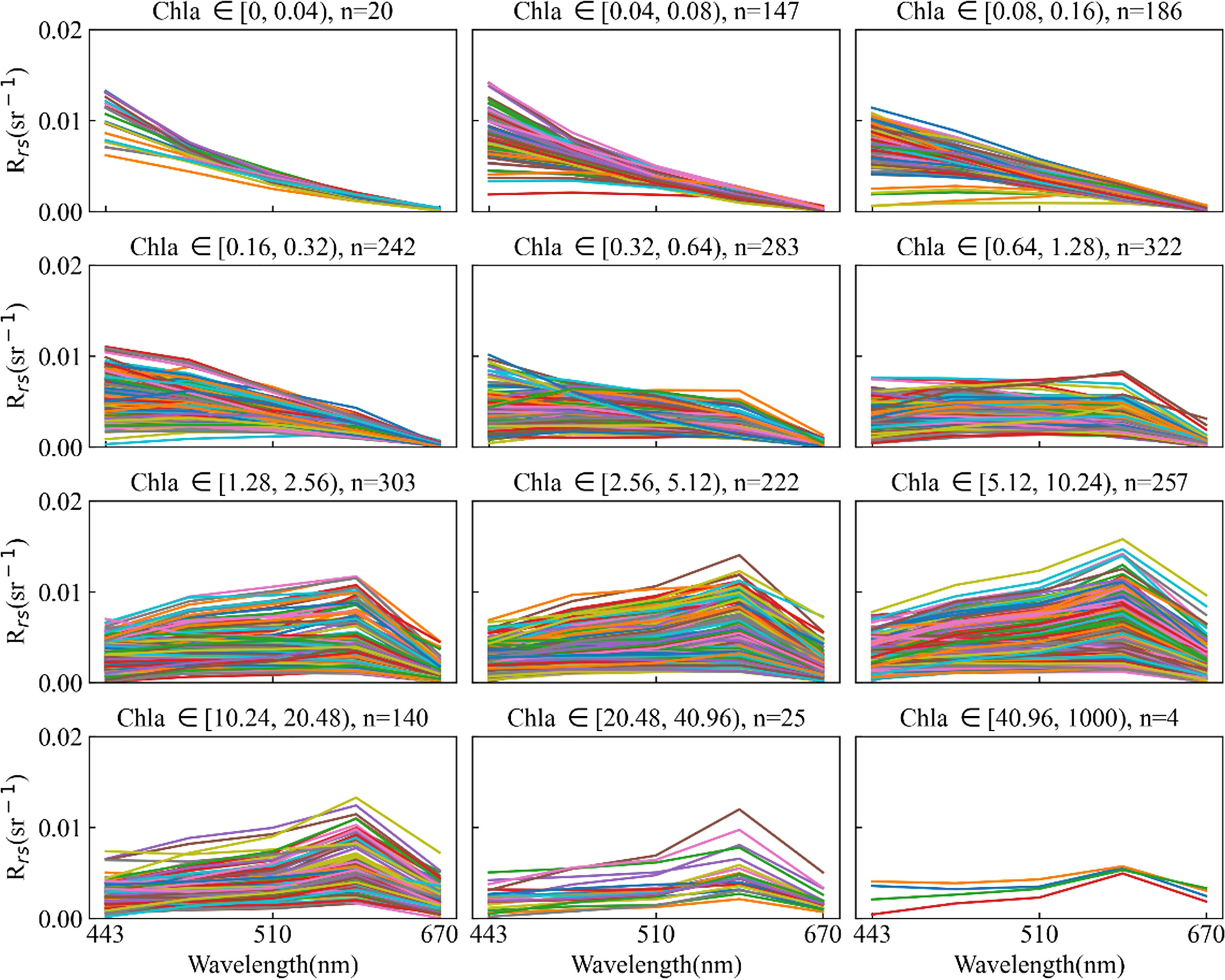
The satellite in situ matchups were separated into 12 range segments according to Chla concentration, and pairs with considerable noise in each range segment were eliminated based on the trend of the spectral curve. We also eliminated pairs containing negative Rrs(λ). After the above steps, the noise points of matchups were removed, which produced a more consistent spectral reflectance curve in the segmented range (Figure 2). SeaWiFS, MERIS, and MODIS-Aqua matchups were reduced to 2151, 611, and 846, respectively. Table 1 shows the in situ Chla concentration statistical information for three sensors after noise rejection. As shown in Figure 2, the peak of spectral reflectance shifted toward the long-wave direction as the chlorophyll concentration increased, which is consistent with the literature (Werdell and Bailey, 2005). Approximately 75% of the matchups were less than 4 mg/m³, and fewer were greater than 20 mg/m³, which resulted in some bias in matchups. We used the log criterion to transform the Chla concentration and remove the bias so that it conformed to the Gaussian distribution (Zhan et al., 2003).

FIGURE 2

Figure 2 Spectral line graph of satellite in situ matchups in different Chla segments of SeaWiFS.

TABLE 1

Table 1 In situ Chla statistical information of three sensors after preprocessing.

The matchups of SeaWiFS were used to assess the CHLNET algorithm. The matchups of MERIS and MODIS-Aqua were used to evaluate the generalization of the CHLNET algorithm on cross-sensor types. Although MODIS-Aqua and MERIS satellite in situ match-up pairs are accessible via the SeaBASS website, it is impossible to directly use match-up pairs for the CHLNET model owing to the difference in the number of bands and center wavelengths. Thus, according to the nearest principle, the Rrs(λ) of MODIS-Aqua and that of MERIS were band-shifted to the input band used by the CHLNET model. The subtle differences in Rrs(λ) caused by sensors are beyond the scope of this paper. Table 2 lists the bands that required band shifting for Aqua and MERIS sensors. The gray cell in Table 2 indicates the band center that would be band-shifted. Band shifting uses Mélin's method (Mélin and Sclep, 2015), which relies on a bio-optical algorithm, namely, the quasi-analytical algorithm (QAA) (Le et al., 2009) to calculate Rrs(λ) at the target band.

TABLE 2

Table 2 Band-shifted bands of MODIS-Aqua and MERIS.

Model development of CHLNET

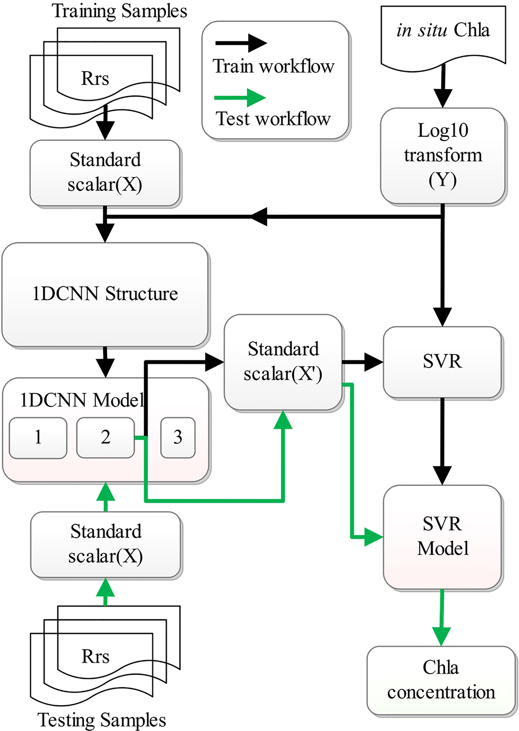
CHLNET consists of a 1D CNN for automatic feature extraction and a regression algorithm for Chla concentration fitting for Chla concentration inversion. Figure 3 shows the framework of CHLNET. Rrs(λ) indicates the remote sensing reflectance in the matchups dataset. The 1D CNN performs feature extraction. We used SVR as a regression algorithm after comparing its performance with other regression algorithms (Supplementary Table S1).

FIGURE 3

Figure 3 Framework of CHLNET.

Feature extraction based on 1D CNN

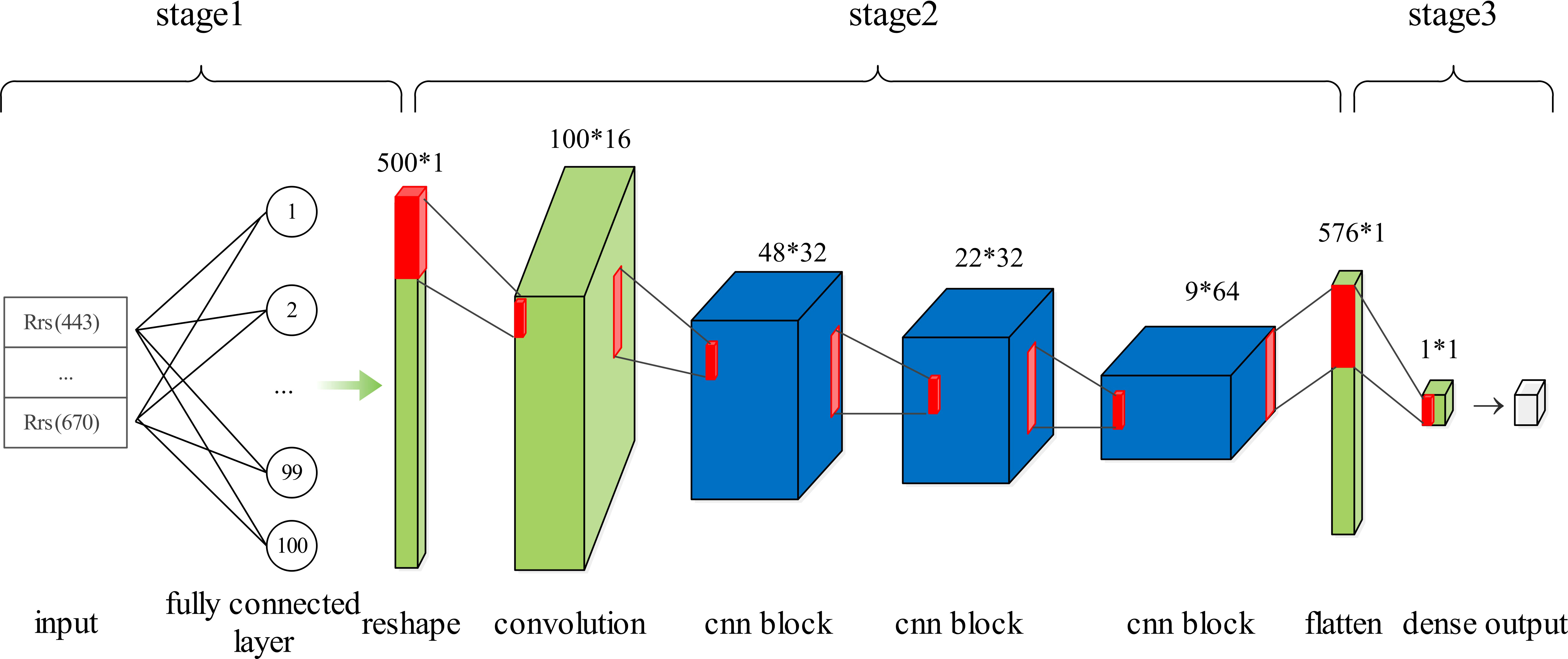
A traditional CNN includes three main elements: a convolutional layer, a pooling layer, and a fully connected layer. The convolutional layer extracts local characteristics from the input features through a convolutional kernel, the output of which is then sampled by the pooling layer. The 1D CNN differs slightly from traditional networks. The input of the convolutional layer is a three-dimensional (3D) vector (samples, time steps, and features), and the output is also a 3D vector (samples, time steps, and channels). Actually, the 1D CNN views the input data as a sequence, on which it can perform convolutional operations. The pooling layer follows the convolutional layer, which is also a 3D vector (samples, time steps, and channels). The pooling layer is used to reduce dimensionality, remove redundant information, and reduce the complexity of the network. Since the original training samples are two-dimensional vectors (samples and features), it is necessary to convert the two-dimensional vector into a 3D vector. It is also desirable to perform a convolution operation to extract more features from a limited number of features (five spectral bands). Too few features limit the number of convolution layers. In this study, there were only five features corresponding to five central bands. Therefore, it is necessary to add input features to meet the quantity requirements of input features for the convolution operation. There are two ways to solve this problem: one way is to repeat features, that is, to simply repeat a feature without changing the feature; for example, the original input vector is (F, 1), and in the case of repeated features, the input vector becomes (F*n, 1), with n denoting the number of repetitions and the other way is to use a fully connected layer for feature addition, such as using a fully connected action of n neuron nodes on the input vector (F, 1), whose output is (F, n), and after performing a reshape operation, the same dimensionality as the first method can be obtained. Both approaches have been tested and have almost the same inversion accuracy. Since the first method requires extra operation, the second method was selected in this study for extending the feature volume. Its structure is shown in Figure 4.

FIGURE 4

Figure 4 1D CNN structure.

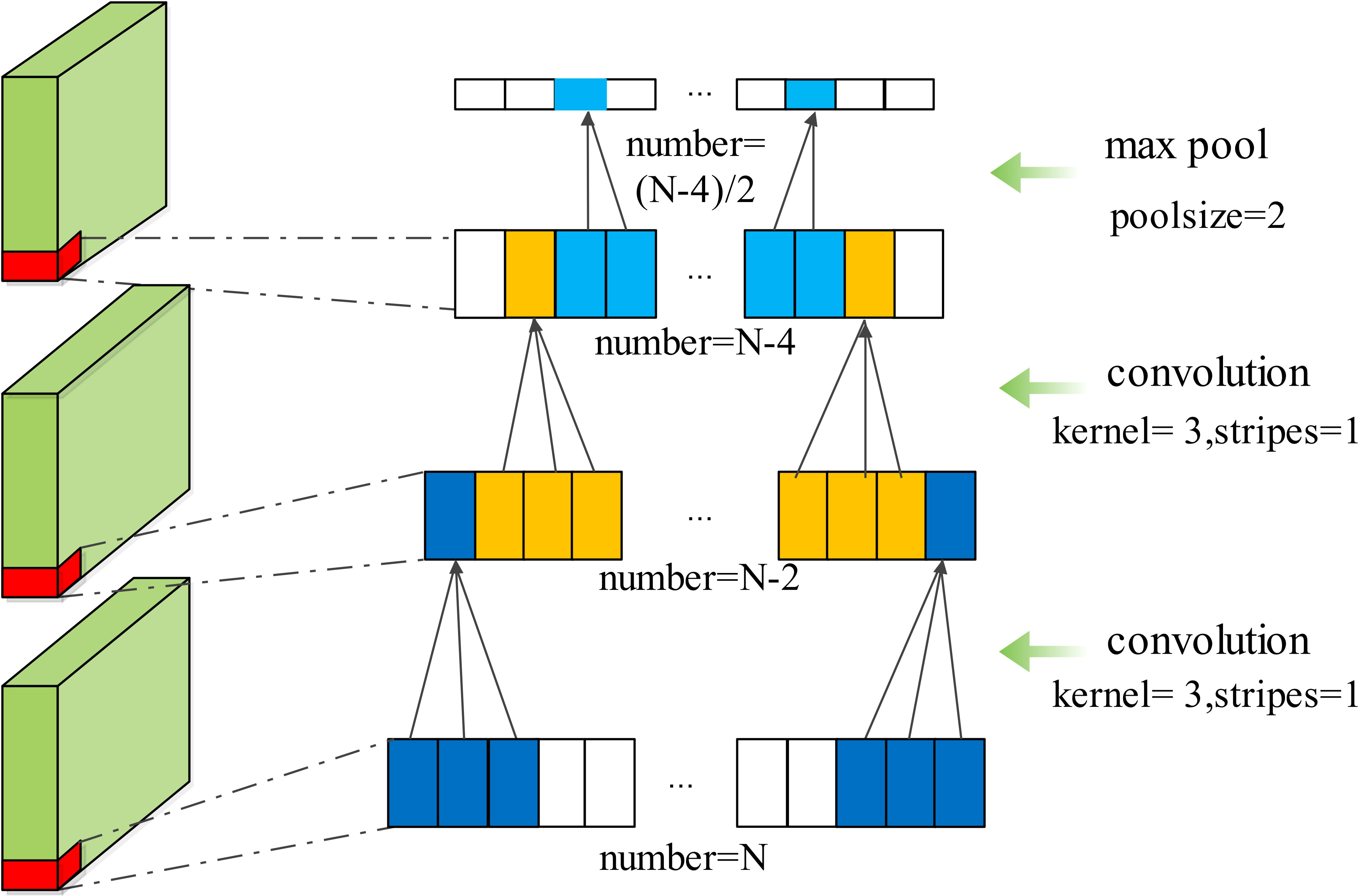
As shown in Figure 4, the 1D CNN is divided into three stages. Stage 1 is the input feature preparation stage, where 500 new input features consisting of original features [Rrs(λ) at 443, 490, 510, 555, and 670 nm] are constructed using the fully connected layer. Stage 2 is the feature extraction stage. As the original number of features is five, a convolutional layer with a convolutional kernel size of 5, strides of 5, and filters of 16 is used to extract 100×16 high-dimensional features. Three CNN blocks follow. Each block consists of two convolutional layers and one pooling layer. In the same block, both convolutional layers have the same parameters, such as kernel size and strides. The pooling layer is calculated according to the maximum pooling, with its pool size set to 2. Figure 5 shows a CNN block where the convolutional kernel size is 3, the stride is 1, and the maximum pooling size is 2. Meanwhile, in each convolutional layer, the activation function is set. The activation function is uniformly set to the ReLU function throughout the 1D CNN network, because the ReLU function showed the best performance during the experiment, as shown in Table 3. Stage 3 is a linear regression that fits the features extracted in Stage 2 to the in situ Chla concentration. The detailed parameters of the 1D CNN are shown in Supplementary Table S2.

FIGURE 5

Figure 5 1D CNN block.

TABLE 3

Table 3 Performance of different activation functions.

Chla inversion workflow of CHLNET

As CHLNET is composed of a 1D CNN and an SVR, its training and testing processes differ from those of conventional neural networks. Therefore, it is necessary to clarify the training and testing processes for CHLNET. During the training phase, five Rrs(λ)s are taken as input features (X), which are input to the 1D CNN for training after normalization. The Chla concentration in log space represents the 1D CNN output (Y). When the model loss settles within an error range around the final value, the 1D CNN completes the training. Then, the outputs of 1D CNN in Stage 2 are normalized to X’, which are used as inputs by the SVR algorithm to fit Chla concentration in log space (Y). During the testing phase, the samples are normalized and predicted with the first two stages of the 1D CNN. The output results are normalized and then input to the SVR model for an estimate to obtain the final prediction results. The training and testing workflow of CHLNET is shown in Figure 6.

FIGURE 6

Figure 6 Chla inversion workflow of CHLNET.

Performance assessment metrics

Standard statistical metrics such as the coefficient of determination (R²), root mean square error (RMSE), and regression slope, are often used to evaluate the accuracy of an inversion algorithm. However, these evaluation metrics are usually applied to Gaussian distribution samples without outliers and are still inadequate in the Chla inversion algorithm (Seegers et al., 2018). Thus, we used the raw and log-transformed Chla metrics for the performance assessment. These metrics included:

$\begin{array}{ll}{R}^2=1-\frac{{\displaystyle {\sum }_{i=1}^n{\left(lo{g}_{10}\left(M_i\right)-lo{g}_{10}\left(E_i\right)\right)}^2}}{{\displaystyle {\sum }_{i=1}^n{\left(\left(lo{g}_{10}\left(M_i\right)-mean(lo{g}_{10}\left(M_i\right)\right)\right)}^2}}& (1)\end{array}$

$\begin{array}{ll}RMSLE=\sqrt{\frac{{\displaystyle {\sum }_{i=1}^n{\left(lo{g}_{10}\left(E_i\right)-lo{g}_{10}\left(M_i\right)\right)}^2}}{n}}& (2)\end{array}$

$\begin{array}{ll}MSE=\sqrt{\frac{{\displaystyle {\sum }_{i=1}^n{\left(E_i-M_i\right)}^2}}{n}}& (3)\end{array}$

$\begin{array}{ll}MAE=10{^}^{\frac{{\displaystyle {\sum }_{i=1}^n\left|lo{g}_{10}\left(E_i\right)-lo{g}_{10}\left(M_i\right)\right|}}{n}}& (4)\end{array}$

$\begin{array}{ll}Bias={10}^{\frac{{\displaystyle {\sum }_{i=1}^{n}lo{g}_{10}\left(E_i\right)-lo{g}_{10}\left(M_i\right)}}{n}}& (5)\end{array}$

The R², root mean squared log error (RMSLE), MAE, and Bias metrics were evaluated in the log-transformed space of Chla. The RMSE was also calculated for Chla without log transformation to assess the standard deviation. The mean absolute error (MAE) was used to quantify the actual error between the estimated Chla and the measured Chla. Slope was used to calculate the linear relationship between estimated Chla and measured Chla in the log-transformed space. The model win percent (MWP) was used to evaluate different Chla inversion models (Seegers et al., 2018).

When there are multiple assessment metrics, it is difficult to judge the pros and cons of the algorithm from one metric. We improved the star plot visualization method proposed by Seegers to evaluate the performance of the algorithm comprehensively. To avoid exaggerating the differences between different metrics, the maximum and minimum of each metric were set according to Equations 6–9, where P_i denotes the ith metric (Chambers et al., 2018). For R², Slope, and MWP, the scalar results could be calculated directly using Equations 6 and 7. For RMSE, RMSLE, and MAE, the smaller the values, the better the performance. The max and min of the scalar were set using Equations 8 and 9, respectively.

$\begin{array}{ll}Maximum=Max\left(P_i\right)+10\%\left(Max\left(P_i\right)-Min\left(P_i\right)\right)& (6)\end{array}$

$\begin{array}{ll}Minimum=Min\left(P_i\right)-10\%\left(Max\left(P_i\right)-Min\left(P_i\right)\right)& (7)\end{array}$

$\begin{array}{ll}Maximu{m}_e=Maximum- Minimum& (8)\end{array}$

$\begin{array}{ll}Minimu{m}_e=0& (9)\end{array}$

Experiments and results

Performance assessment of CHLNET

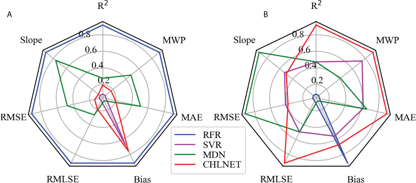
To evaluate the performance metrics of the CHLNET model, RFR, SVR (Hu et al., 2020), and MDN were used for comparison. Because SeaWiFS L3 Chla product data were derived from the OC4 and CI algorithms, the performance results of OC4 and CI algorithms were no longer listed. The SeaWiFS Chla product data were listed as a comparative analysis. In machine learning algorithms, input features can directly affect the model's accuracy. Hu et al. (2020) extended the original features when applying the SVR algorithm to the inverse of ocean surface Chla. So, in this paper, we followed Hu's method for feature extension, using the raw spectral features and extended features to train and evaluate the RFR and SVR models. The matchups of SeaWiFS were split into training and testing datasets according to the ratio of 7:3. All algorithms use the same training data (n = 1505) and testing data (n = 646). Table 4 lists the performance metrics of these algorithms. We normalized the performance metrics of the four algorithms on the whole dataset and testing dataset according to the comprehensive evaluation method in Section 3.3, using the SeaWiFS Chla product metric as the baseline. Figure 7 shows the Seegers plot based on the normalized results for whole dataset and testing dataset.

TABLE 4

Table 4 Performance metrics of different algorithms on whole dataset and testing dataset.

FIGURE 7

Figure 7 Comparison of seven metrics in the star plot on the whole (A) and testing dataset (B).

Because the inputs of SVR and RFR are merged features of original Rrs(λ)s and extended features that are based on the band ratio and band difference, the performance metrics of the two algorithms in this paper were higher than those of the SeaWiFS Chla product. Some metrics were even higher than those of the neural network (MDN and CHLNET) algorithms, such as the bias of SVR. RFR covered the largest area on the whole dataset, but it covered only a small area on the testing dataset, indicating the overfitting of RFR on the training data. In Hu et al.’s study, SVR showed better performance, which is also corroborated by this paper, where SVR was second only to CHLNET in terms of the coverage area on the testing dataset. Overall, SVR and RFR outperformed the SeaWiFS Chla product, showing that when extended features are available, the SVR and RFR algorithms have the capability of inversing Chla.

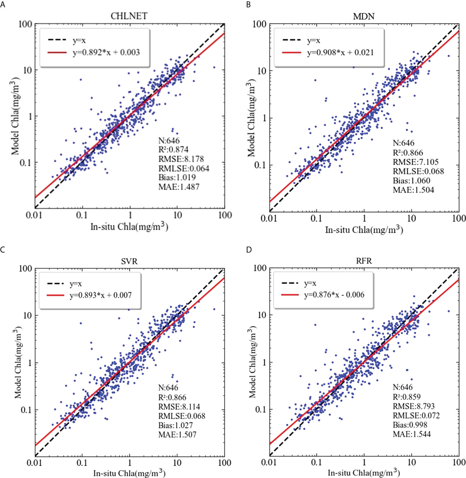
The MDN used in the experiment consists of one input layer (n = 5), five hidden layers (n = 100), one mixture layer, and one output layer. From Table 4, the performance metrics Slope and RMSE of MDN were the best performers, which outperformed those of the other four algorithms. However, in terms of real metric values, the Slope and RMSE metrics of CHLNET were close to the values of MDN, and the difference between them was only 0.016 in Slope and 1.073 mg/m³ in RMSE on the testing dataset. CHLNET showed good performance on the testing dataset, outperforming the other four algorithms in several metrics (e.g., R², MWP, and MAE). From the scatter plot (Figure 8), we can see that there was an overestimation of low Chla concentration and an underestimation of high Chla concentration for all algorithms (Slope < 1). These four algorithms were very close to each other in scatter morphology on the testing dataset. Table 4 shows that the CHLNET outperformed the SVR and RFR, which indicates that the CHLNET without feature extension provides a novel perspective on Chla inversion.

FIGURE 8

Figure 8 Scatter plot of CHLNET (A), MDN (B), SVR (C) and RFR (D) on the testing dataset.

Evaluation of CHLNET performance at different trophic levels

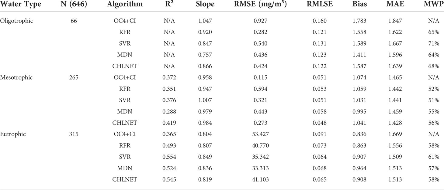
To further analyze the accuracy of CHLNET at different Chla concentrations, the testing dataset was divided into three trophic levels, defined as oligotrophic (Chla ≤ 0.1 mg/m3), mesotrophic (0.1 < Chla ≤1 mg/m3), and eutrophic (Chla > 1 mg/m3) (Seegers et al., 2018). Table 5 lists the performance metrics on the testing dataset for each trophic level. For oligotrophic waters, although CHLNET was not the optimal model, its performance metrics (RMSE, RMSLE, MAE, and MWP) were the second best. Bias metrics for all models were greater than 1, which indicates that all models overestimate for oligotrophic waters. For mesotrophic waters, CHLNET outperformed other models on almost every metric, except for the Bias metric (1.041), which is slightly lower than that of MDN (0.995) and SVR (1.031). The Slope metric improved from 0.866 to 0.984. The Bias metric was closer to 1, moving from 1.587 to 1.041. This indicates that the predicted Chla concentrations are more evenly distributed on both sides of the in situ measurements at this trophic level. CHLNET also offered performance advantages at the eutrophic level compared to other models. The R², RMSLE, Bias, MAE and MWP of CHLNET had the second-best performance. In Figure 9, the Chla frequency distribution of CHLNET and SVR was significantly better than that of the other models. As the frequency distribution plots of Chla concentration of SVR and CHLNET seem to be similar, it is difficult to directly infer which model is better. However, in Table 4, the MAE metric of CHLNET (1.487) was slightly lower than that of SVR (1.504). Therefore, CHLNET at the three trophic levels is more consistent with the in situ measurements. Based on the results it can be concluded that CHLNET exhibits higher inversion accuracy at different trophic levels and avoids the problem of combining OWT-based inversions to establish a consistent inversion model of Chla.

TABLE 5

Table 5 Performance metrics for different trophic levels.

FIGURE 9

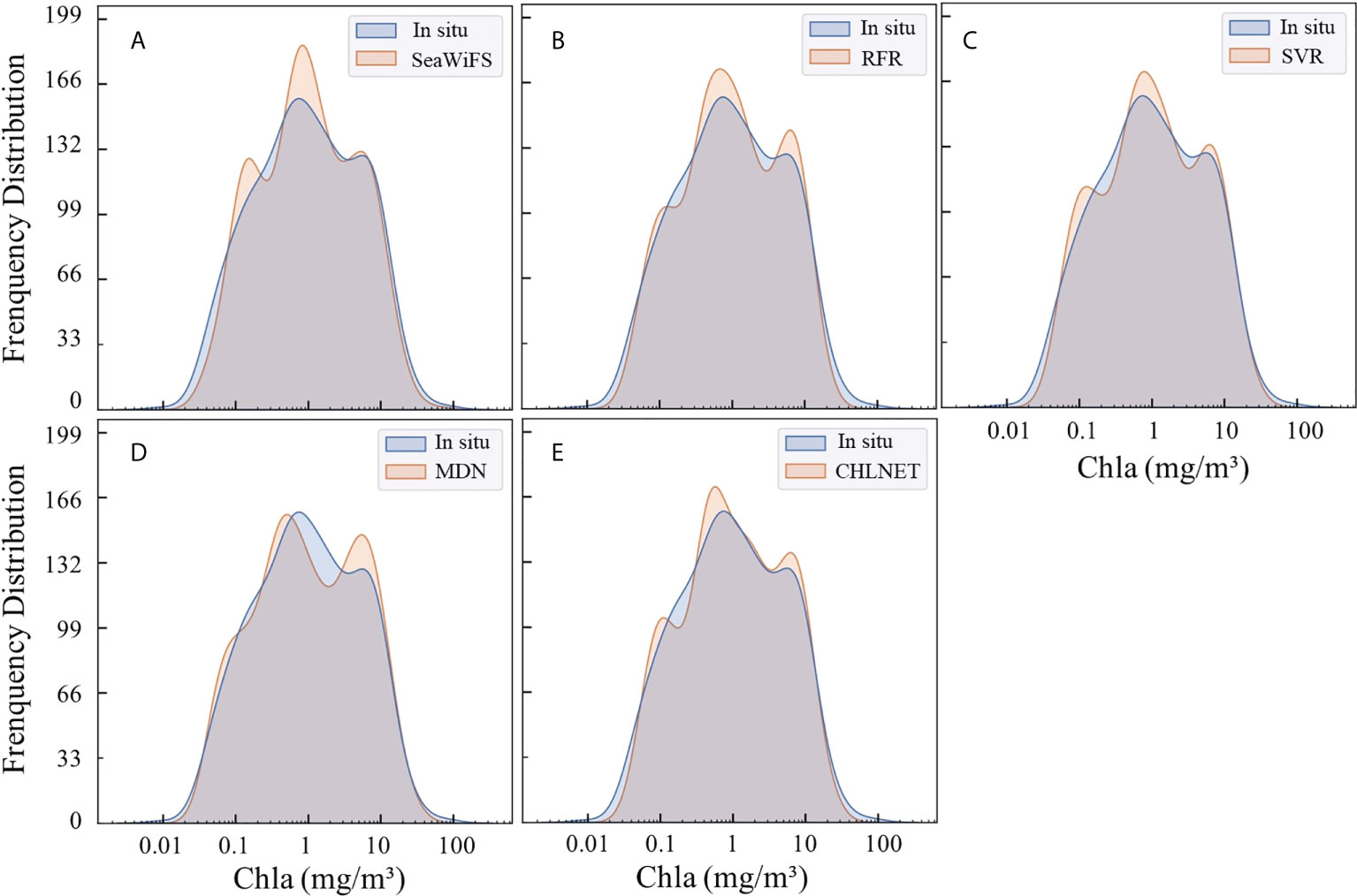
Figure 9 Predicted Chla frequency distribution of SeaWiFS (A), RFR (B), SVR (C), MDN (D), and CHLNET (E) on the testing dataset.

Spatial mapping capability of CHLNET

The spatial mapping capability of CHLNET was verified at two time scales: one is the monthly average (June 2010) Chla concentration, and the other is the 8-day (24–31 October 2010) fused Chla concentration. Figures 10C–F show the SeaWiFS global Chla distributions derived from CHLNET and SVR algorithms. SeaWiFS Chla product data (Figures 10A, B) from the same period were used as a comparison. For Chla concentration mapping on two time scales, the inversion results of CHLNET, SVR, and SeaWiFS products have similar spatial patterns. Large-scale oceanic elements, such as upwelling near the Equator and the phenomenon of high Chla concentration in coastal waters, could be seen. Although there were some differences in the performance of CHLNET, SVR, and SeaWiFS, as shown in Table 4, such differences would be difficult to be observed at large-scale global Chla concentrations. Therefore, we compared the Chla concentration of CHLNET, SVR, and SeaWiFS from three latitudes (30°N, 0°, 30°S). Figure 11 shows the scatter plots of the concentrations in the range of −180° to 180° for the three latitudes and the difference plots (Diff = CHLNET/MDN−SeaWiFS). For simplicity, only differences in the range of −0.5 (mg/m³) to 0.5 (mg/m³) are retained in Figure 11. The differences in Chla of both CHLNET and SVR at latitude 30°N, 30°S (Figures 11A, C) show a consistent fluctuation pattern; that is, the estimated Chla was generally higher than that of SeaWiFS in the open ocean (difference > 0). The estimated Chla was generally lower than that of SeaWiFS in the coastal waters (difference < 0). The differences on the equatorial line (Figures 11B) had a significant fluctuation. However, there were some subtle differences in CHLNET and SVR. Although the differences in CHLNET were bigger than SVR’s on the Equator, it is hard to conclude that SVR mapping results were better, due to the lack of ground truth. In oligotrophic waters (Chla < 0.1 mg/m³), the Chla values assessed by CHLNET showed dispersion (green scatter points for Chla < 0.1 mg/m³ in Figures 11A). This result is consistent with the evaluation of oligotrophic waters in Figure 9 based on in situ measurements.

FIGURE 10

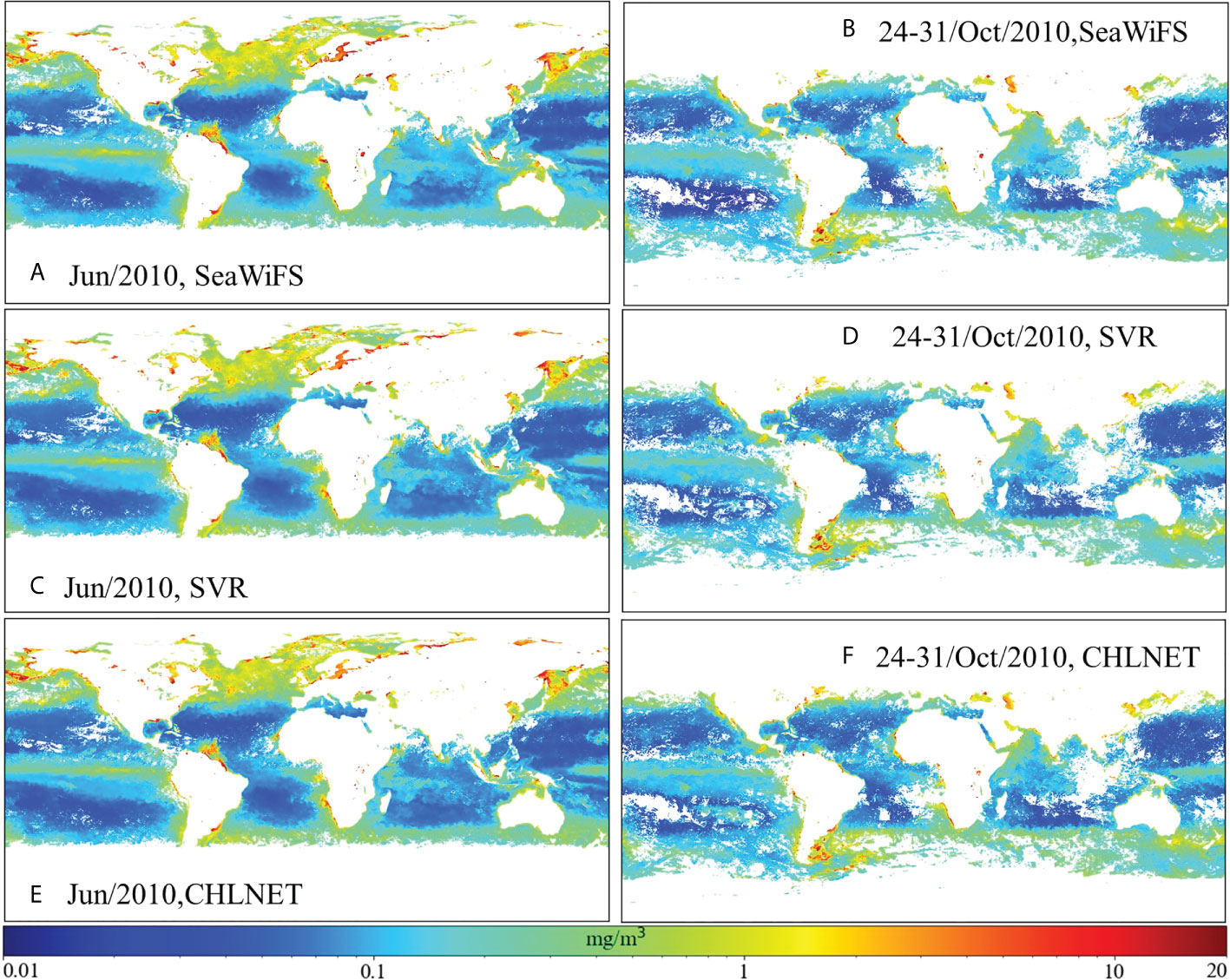
Figure 10 (A, B) SeaWiFS Chla distribution, (C, D) SVR Chla distribution, and (E, F) CHLNET Chla distribution of the global map on monthly and 8-day scales.

FIGURE 11

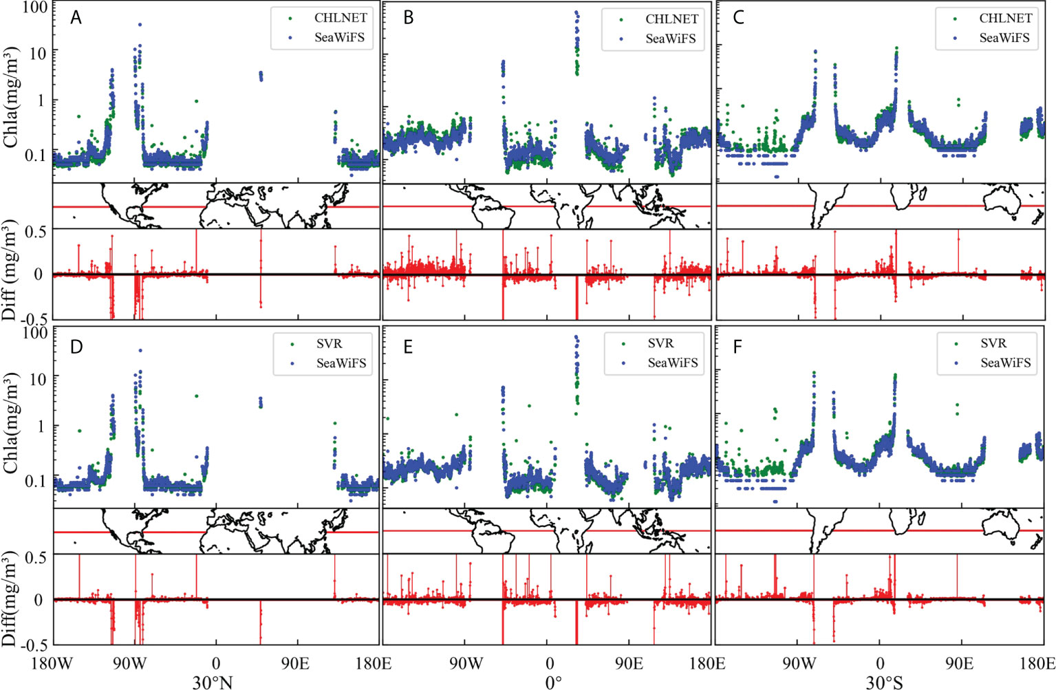
Figure 11 (A–F) indicate the scatter plot of CHLNET, MDN, and SeaWiFS Chla distribution at 30N°, 0°, and 30°S, respectively, on an 8-day scale (24–31 October 2010).

The eastern waters of Tasman Asia, Australia (147°–156°E, 49°–38°S) in the southern hemisphere were selected for further analysis of CHLNET performance at local scales (as shown in Figure 12) because of the occurrence of mesotrophic and eutrophic waters in this region. The MODIS-Aqua Chla product from NASA in this region was introduced as the reference to observe more detailed Chla spatial patterns because of its higher spatial resolution than SeaWiFS. CHLNET (Figure 12C) and SVR (Figure 12B) have nearly consistent spatial patterns. Compared with SeaWiFS data (Figure 12A), the CHLNET data are smoother and almost contain no noise points at the same spatial resolution in the open ocean (pale blue ellipse), indicating that CHLNET has a higher noise tolerance. In the coastal region (blue ellipse), CHLNET data are higher than those of the SeaWiFS and MODIS-Aqua Chla product, and changes in Chla concentration are smoother throughout this region. In another open ocean (red ellipse), Chla concentration of MODIS-Aqua generally had higher Chla values, with the highest values occurring at the bottom of this region. Compared to the SeaWiFS Chla product, the distribution of CHLNET Chla concentration was more similar to that of the MODIS-Aqua Chla product, indicating that even at a low spatial resolution (9 km), CHLNET can still capture detailed changes. In addition, the MODIS-Aqua Chla product showed a striped distribution (black ellipse), and CHLNET represents the Chla distribution in this region. In contrast, SeaWiFS showed a break and low Chla concentration in the middle part.

FIGURE 12

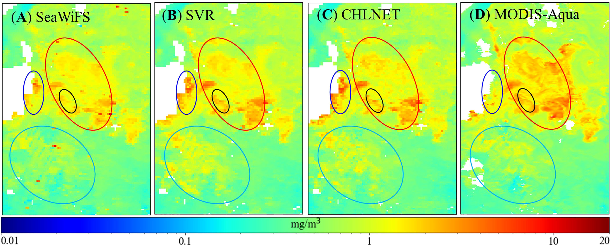
Figure 12 Comparison of region (147°–156°E, 49°–38°S) Chla distribution of the SeaWiFS product (9 km) (A), SVR model (9 km) (B), CHLNET model (9 km) (C), and MODIS-Aqua product (4 km) (D) on 24–31 October 2010.

The eastern U.S. coastal region in the northern hemisphere was selected for further analysis of CHLNET’s mapping capabilities at low Chla concentrations, which was used by Hu in developing the OCI algorithm. Figure 13 shows the mapping results of Chla concentrations in this region. In eutrophic waters (blue ellipse), the spatial pattern of Chla concentration was different for the four data. CHLNET’s Chla concentrations showed a smooth transition, unlike MODIS-Aqua’s Chla concentrations, which suddenly rose from the northeast to the southwest, as well as the Chla concentrations of both SeaWiFS and SVR, which had high values. In oligotrophic waters, CHLNET’s Chla spatial pattern no longer exhibited smoothness (red ellipse). The CHLNET model generally shows excellent mapping performance in mesotrophic and eutrophic waters. However, the mapping ability at low Chla concentrations could be improved.

FIGURE 13

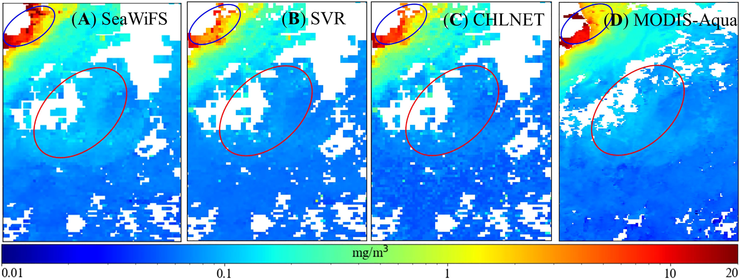
Figure 13 Comparison of region (76.6°–70.5°W, 28.5°–36.5°N) Chla distribution of the SeaWiFS product (9 km) (A), SVR model (9 km) (B), CHLNET model (9 km) (C), and MODIS-Aqua product (4 km) (D) on 24–31 October 2010.

Generalization of CHLNET on cross-sensor

In addition to accuracy, the CHLNET model was evaluated for its ability to generalize across sensors, rather than sensor-specific algorithms. To quantify the generalization ability of the CHLNET model on cross-sensor data, the satellite in situ matchups of MERIS and MODIS-Aqua after band shifting were split into training and testing datasets in the ratio of 7:3. The CHLNET model trained on the SeaWiFS dataset was applied to the MERIS and MODIS-Aqua testing datasets. Table 6 shows the performance metrics of the two sensors. CHLNETseawifs denotes the CHLNET model trained on SeaWiFS matchups. Product denotes the OCx algorithm used to generate the Chla product. In addition, we wanted to investigate how the model’s accuracy changes when a specific sensor sample is covered.

TABLE 6

Table 6 Performance metrics of cross-sensor.

From Table 6, it can be seen that the CHLNETseawifs could still achieve good performance metrics in the cross-sensor Chla inversion, indicating that the CHLNETseawifs captures some of the spectral features when applied to new sensor data and has certain generalization ability. For the MERIS testing dataset, except for the Slope metric, which was slightly smaller, the performance metrics of CHLNETseawifs were better than the MERIS Chla product accuracy. For the MODIS-Aqua testing dataset, the accuracy of the CHLNETseawifs model was greater than that for the Chla product, but the difference was small (MWP = 51%). Note that the Slope metric of the CHLNETseawifs was low (Slope = 0.728). This is because the model overestimated Chla concentration at the oligotrophic level and underestimated it at the eutrophic level. As a result, R2 was larger (0.859), while the Slope was lower.

For horizontal comparison, a cross-sensor inversion model was built, called CHLNETcross, based on the CHLNETseawifs model using 70% match-up pairs of MERIS and MODIS-Aqua. Compared to the CHLNETseawifs, CHLNETcross performance metrics were improved. The performance improvement of the CHLNETcross model on the MODIS-Aqua testing dataset was significantly greater than that of MERIS. For example, on the R² metric, the performance of MODIS-Aqua increased by 6%, while that of MERIS increased by only 2%. This phenomenon might be because the band to be band-shifted in MODIS-Aqua was too far (~21 nm) from the target band, resulting in a significant error after the band shift. After the addition of match-up samples from MODIS-Aqua, the CHLNET model filled the gap that failed to capture the features for this sensor, and the model accuracy was immediately improved. The above results demonstrate that the CHLNETseawifs can capture the standard spectral features of cross-sensor types. With the addition of specific sensor samples, the CHLNETcross captured some features on the MERIS and MODIS-Aqua testing datasets that CHLNETseawifs did not extract. This demonstrates that the CHLNET model can be applied for cross-sensor generalization when the target sensor samples are insufficient for building CNN models.

Discussion

Feature extension effect on the performance of CHLNET

The CNN is excellent at detecting simple patterns in data and then in leveraging those simple patterns to produce more complex patterns in higher layers. In the Chla inversion model, the Rrs(λ) can be viewed as a shorter sequence with a fixed length. Then, the 1D CNN can extract features efficiently from such a sequence segment. Therefore, we designed the first layer of the CHLNET network with a kernel size of 5 and a stride of 5. Under this convolution layer, each newly extracted feature combines five bands [Rrs(λ) at 443, 490, 510, 555, and 610 nm]. This concept is similar to the classical concept of combining through bands (two- or three-band combination). Based on this, when creating the network structure, this paper employs 1D CNN to extract features and SVR as a regression algorithm for Chla fitting, and the two combine to form the new model, CHLNET. The difference is that the CHLNET model learns the weights of the band combinations through convolutional networks. Through multiple iterations, the model learns the mathematical form similar to the band combination to realize the inversion of Chla.

To determine whether the CHLNET model can learn the band combination or higher-dimensional features, we added extended features into the input to observe the change in CHLNET performance. To simplify the work, we only discuss the R² and MAE performance metrics. In order to prevent the influence of random noise, the performance metrics were recorded at a median value of 20 times when a new feature was added. Figure 14 shows the changes in the R² and MAE metrics when the input features increased. o denotes the original band feature, e denotes the extended feature, and the detailed description of each feature combination is shown in Supplementary Table S3. For comparison, we performed 3 experiments on the original band features (o, o1, and o2) and 11 experiments on the extended feature combinations. As illustrated in Figure 14, when features were added, except for metrics that fluctuated in the training dataset (solid line), there was little change in the testing dataset (dash line). The metrics when o was used as the input feature were treated as the baseline in Figure 14, and the metrics of different input features were subtracted from this baseline as difference. The maximum change in R² was found to be 0.007, while the maximum change in MAE was 0.011. The amount of change compared to the original metric value was essentially negligible. This indicates that the introduction of extended features hardly improves the accuracy of CHLNET, thus verifying that CHLNET is capable of extracting more complex or high-dimensional features from simple bands [Rrs(λ)].

FIGURE 14

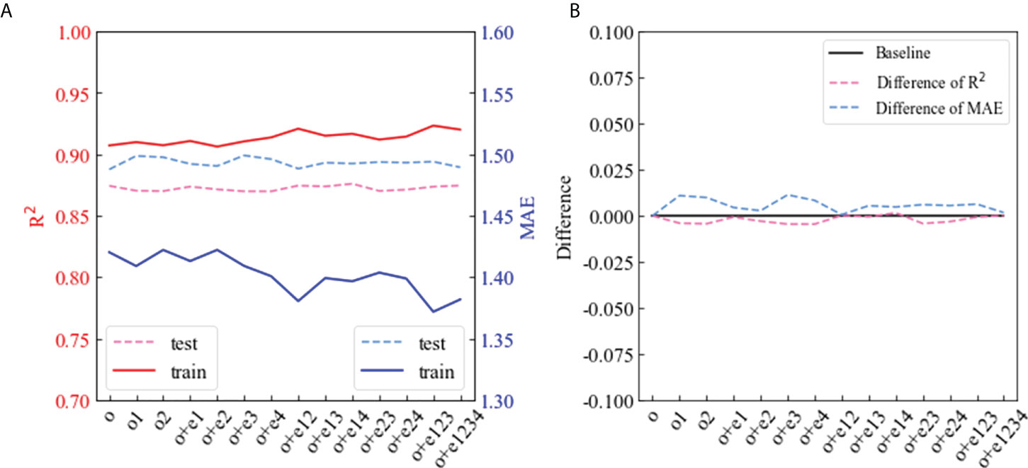
Figure 14 Effect of different input features on R² and MAE metrics of CHLNET. (A) represents the change of R² and MAE when input features have changed. (B) indicates the metric variation of R² and MAE using the accuracy of origin input features as the baseline.

Effect of network structure on model convergence for Chla inversion

MDN can implement one-to-many inversion, that is, the same input can output multiple different values. In recent years, the model has been frequently used for regression applications with multiple normal distribution patterns (Pahlevan et al., 2020; Smith et al., 2021). MDN is a combined model based on MLP and Gaussian Mixture Model (GMM). GMM consists of several Gaussian components. MLP is responsible for extracting each Gaussian component's weight, variance, and mean. Prediction output is based on the mixture weights and the morphology of Gaussian components, which enables MDN to predict multiple outputs based on the same input. In this paper, we propose CHLNET, combining 1DCNN and SVR. CHLNET and MDN have many similarities: both models are ensemble models; the former is MLP+GMM, and the latter is 1D CNN+SVR; moreover, the input features of the models are original features; so, there is no need to extend the features. MLP and 1D CNN play a similar role in the overall model, that is, feature extraction. From the experimental results (Table 4), it can be noted that both MLP and 1D CNN obtained better performance and played an essential role in completing the feature extraction. However, the following questions need further discussion: what is the difference between the two structures? Which network structure should be chosen when inversing Chla.

Theoretically, there is a fundamental difference between how MLP and 1D CNN extract features. As MLP is a fully connected form, one fully connected layer can extract features consisting of different numbers of bands. If there are five input feature bands and 100 neurons in hidden layer (Figure 15A), and if the weights w₁₁, w₁₂, and w₁₃ tend to 0, then the X₁ feature consists of two bands, Rrs (555) and Rrs (670). Similarly, X₁ can also be composed of any three or four bands. However,1D CNN networks perform feature extraction by way of convolution. Figure 15B shows the case of extracting features consisting of two bands with a convolution kernel size of 2, and a stride of 1. It shows that the number of parameters used by the 1D CNN to extract features was less than that of MLP. In an extreme case, when extracting 100 new features consisting of two bands, in the structure shown in Figure 15B, the MLP required 5 × 100 = 500 parameters, while the 1D CNN required only 2 × 100 = 200 parameters. We built a five-layer network structure using MLP and 1D CNN, where the MLP consisted of five fully connected layers and the 1D CNN consisted of five CNN layers. The impact of parameter increases on model loss can be observed by increasing the network parameters by changing the number of neurons in the hidden layer (1D CNN is the number of channels). Figure 15C shows the changes in the loss metric on the training dataset when the MLP and 1D CNN network parameters increased. The loss of the 1D CNN stabilized at 5000 parameters, while the loss of MLP stabilized at 10,000 parameters. The 1D CNN could stabilize the loss with one and a half fewer parameters than MLP. Therefore, the 1D CNN could achieve the expected inversion results with a smaller network structure compared to MLP networks. Thus, it can be inferred that CNN networks can be widely used in water color remote sensing inversion, especially when the number of samples is limited.

FIGURE 15

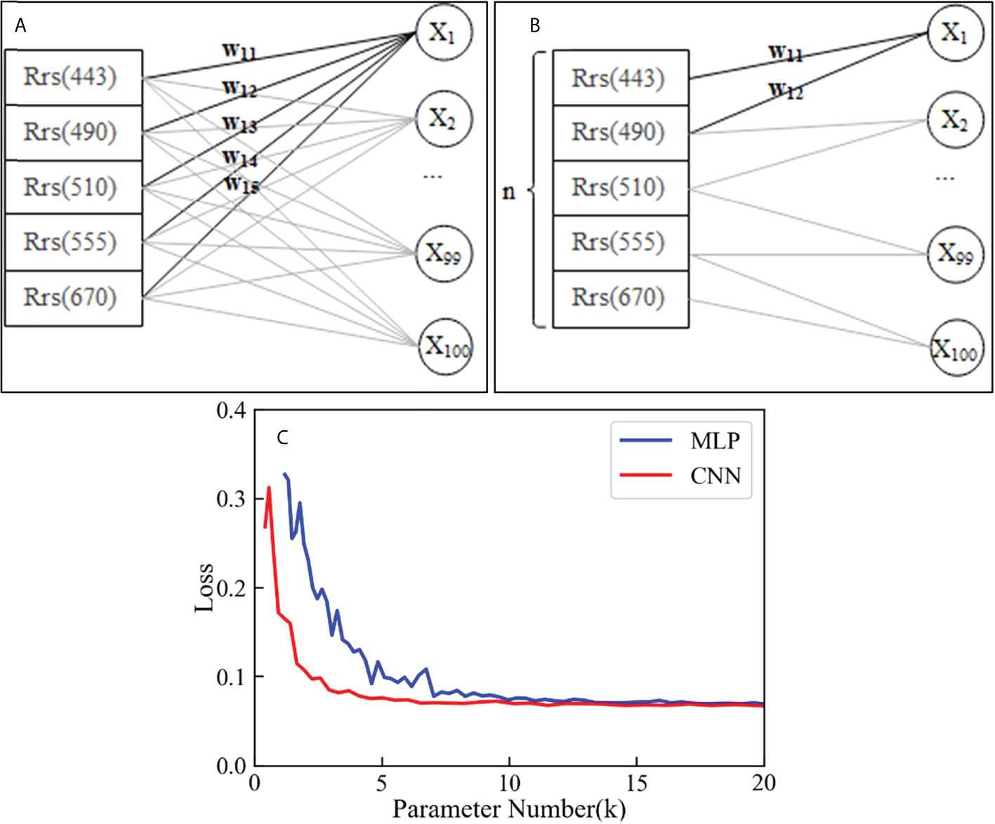
Figure 15 Feature extraction diagram of MLP (A), 1D CNN (B), and loss change with increasing parameter number (C).

Capability of CHLNET

CHLNET is an empirical model obtained by training based on in situ measurements. Therefore, it also has the pros and cons of an empirical model. As CHLNET does not have an explicit functional form, it is impossible to determine the physical meaning of the features. Therefore, obtaining Chla accuracy beyond the training range is challenging when the training data are insufficient. Greater attention should be paid to the CHLNET model when Chla exceeds the training range. In Table 5 and Figure 9, the limited inversion capability of CHLNET in low Chla concentration waters would overestimate the Chla concentrations. When performing global Chla mapping, discrete noise points appeared (Figures 11E, F). However, this does not mean that the model cannot be used for low concentration Chla inversion. CHLNET performance metrics (Supplementary Figure S4) outperformed the model built on the whole dataset when the model was trained individually on different trophic level samples (Table 5). From Supplementary Figure S4, it can be seen that the overestimation and underestimation of the CHLNET model occurred at the head and tail of the training dataset, respectively. They were not related to the trophic level, which is an inherent flaw of the model. Therefore, when applying the CHLENT model, attention needs to be paid to the range where the Chla concentrations are in the head and tail of the training dataset.

CHLNET could perform better than the OCx algorithm for cross-sensor applications (Table 6), which provides a new idea for the retrieval of Chla. When the sensor sample size is limited, CHLNET’s feature extraction weights learned in the original sensor (e.g., SeaWiFS matchups) can be transferred to the new sensor (e.g., MERIS matchups) via transfer learning. A small number of new sensor samples can be used to optimize the original CHLNET and establish high-performance inversion capabilities of the target sensor. For example, the performance of CHLNETcross, as shown in Table 6, was better than that of CHLNETseawifs. However, it should be noted that the capability of the cross-sensor model was affected by the band-shift algorithm. In Table 6, the performance metrics of the CHLNETseawifs model on the MERIS testing dataset were significantly better than the performance metrics on the MODIS-Aqua testing dataset. The reason for this result might be that the MERIS sensor only needs two bands (560 nm and 665 nm) for the band shift. The band center was close to the SeaWiFS band center (555 nm and 670 nm), while the MODIS-Aqua sensor required three band shifts (488 nm, 531 nm, and 667 nm), and the center bands of 531 nm and 510 nm were far from each other, which might cause a more significant error. Supplementary Table S5 shows the performance results for cross-sensor applications with the original bands of MERIS and MODIS-Aqua as input features of CHLNET. It can be seen that without band shifting, the performance of MODIS-Aqua was significantly reduced. For instance, R² of the testing dataset was reduced from 0.859, 0.894 to 0.838, 0.889 on model CHLNETseawifs and CHLNETcross, respectively. Therefore, attention should be paid to the impact of the accuracy of the band-shift algorithm on the accuracy of the cross-sensor model based on CHLNET.

Conclusion

In this study, we developed a new model for ocean surface Chla inversion using the SeaWiFS Chla validation dataset provided by SeaBASS. The performance assessment demonstrated that the CHLNET algorithm performed better than the state-of-the-art algorithms, namely, OCx, SVR, RFR, and MDN algorithms. Application on different trophic waters indicates that CHLNET avoids the need to combine OWT-based inverse algorithms to establish a unified inversion model for Chla across various water types. The Chla mappings on global and local scales illustrate the quality of the spatial pattern. Although performance was slightly poor when mapping oligotrophic waters, CHLNET inversion results in coastal waters were more realistic and showed richer details and higher tolerance to noise. The generalization applications on MERIS and MOIDS-Aqua satellite–in situ matchups indicate that CHLNET can significantly improve the performance of CHLNET in cross-sensor Chla inversion by adding a small number of target sensor matchups to the training dataset. Therefore, CHLNET can serve as an alternative approach for ocean surface Chla concentration retrievals. With the widespread implementation of multispectral and hyperspectral satellites, the hybrid algorithm of the inversion of Chla based on the 1D CNN and SVR to extract high-dimensional features from raw Rrs(λ) can be a new approach to inverse more bio-optical properties.

Data availability statement

The original contributions presented in the study are included in the article/Supplementary Material. Further inquiries can be directed to the corresponding authors.

Author contributions

DF conceived the study; DF, HH, RW, and LL contributed to methodology. BF, YXi, and EG participated in the data elaboration and data curation. DF drafted the first version of the manuscript. HH, RW, YZ, and YXu participated in the manuscript preparation and improvement. All authors contributed to manuscript preparation and to the final version.

Funding

This study was supported by the Natural Science Foundation of Guangxi Province (CN) (2022GXNSFBA035637), the Basic Scientific Research Ability Improvement Project for Young and Middle-aged Teachers of Universities in Guangxi (2021KY0255), the National Natural Science Foundation of China (41801071), and the “BaGui Scholars” program of the provincial government of Guangxi.

Acknowledgments

The authors thank all researchers who contributed to the NASA NOMAN dataset and SeaBASS data achieved. We also appreciate the reviewers for their comments and suggestions, which helped to improve the quality of this manuscript.

Conflict of interest

The authors declare that the research was conducted in the absence of any commercial or financial relationships that could be construed as a potential conflict of interest.

Publisher’s note

All claims expressed in this article are solely those of the authors and do not necessarily represent those of their affiliated organizations, or those of the publisher, the editors and the reviewers. Any product that may be evaluated in this article, or claim that may be made by its manufacturer, is not guaranteed or endorsed by the publisher.

Supplementary material

The Supplementary Material for this article can be found online at: https://www.frontiersin.org/articles/10.3389/fmars.2022.934536/full#supplementary-material

References

Asim M., Brekke C., Mahmood A., Eltoft T., Reigstad M. (2021). Improving chlorophyll-a estimation from sentinel-2 (MSI) in the barents Sea using machine learning. IEEE J. Select. Top. Appl. Earth Observat. Remote Sens. 14, 5529–5549. doi: 10.1109/JSTARS.2021.3074975

CrossRef Full Text | Google Scholar

Awad M. (2014). Sea Water chlorophyll-a estimation using hyperspectral images and supervised artificial neural network. Ecol. Inf. 24, 60–68. doi: 10.1016/j.ecoinf.2014.07.004

CrossRef Full Text | Google Scholar

Bailey S. W., Werdell P. J. (2006). A multi-sensor approach for the on-orbit validation of ocean color satellite data products. Remote Sens. Environ. 102 (1-2), 12–23. doi: 10.1016/j.rse.2006.01.015

CrossRef Full Text | Google Scholar

Chambers J. M., Cleveland W. S., Kleiner B., Tukey P. A. (2018). Graphical methods for data analysis (New York: Chapman and Hall/CRC).

Google Scholar

Cheng Y., Bhoot V. N., Kumbier K., Sison-Mangus M. P., Brown J. B., Kudela R., et al. (2021). A novel random forest approach to revealing interactions and controls on chlorophyll concentration and bacterial communities during coastal phytoplankton blooms. Sci. Rep. 11 (1), 1–11. doi: 10.1038/s41598-021-98110-9

PubMed Abstract | CrossRef Full Text | Google Scholar

D'Alimonte D., Zibordi G., Berthon J.-F., Canuti E., Kajiyama T. (2012). Performance and applicability of bio-optical algorithms in different European seas. Remote Sens. Environ. 124, 402–412. doi: 10.1016/j.rse.2012.05.022

CrossRef Full Text | Google Scholar

Dierssen H. M. (2010). Perspectives on empirical approaches for ocean color remote sensing of chlorophyll in a changing climate. Proc. Natl. Acad. Sci. 107 (40), 17073–17078. doi: 10.1073/pnas.0913800107

CrossRef Full Text | Google Scholar

Doerffer R., Schiller H. (2007). The MERIS case 2 water algorithm. Int. J. Remote Sens. 28 (3-4), 517–535. doi: 10.1080/01431160600821127

CrossRef Full Text | Google Scholar

Gitelson A. (1992). The peak near 700 nm on radiance spectra of algae and water: relationships of its magnitude and position with chlorophyll concentration. Int. J. Remote Sens. 13 (17), 3367–3373. doi: 10.1080/01431169208904125

CrossRef Full Text | Google Scholar

Gitelson A. A., Schalles J. F., Hladik C. M. (2007). Remote chlorophyll-a retrieval in turbid, productive estuaries: Chesapeake bay case study. Remote Sens. Environ. 109 (4), 464–472. doi: 10.1016/j.rse.2007.01.016

CrossRef Full Text | Google Scholar

Gower J. (2016). On the use of satellite-measured chlorophyll fluorescence for monitoring coastal waters. Int. J. Remote Sens. 37 (9), 2077–2086. doi: 10.1080/01431161.2015.1111542

CrossRef Full Text | Google Scholar

Hafeez S., Wong M. S., Ho H. C., Nazeer M., Nichol J., Abbas S., et al. (2019). Comparison of machine learning algorithms for retrieval of water quality indicators in case-II waters: A case study of Hong Kong. Remote Sens. 11 (6), 617. doi: 10.3390/rs11060617

CrossRef Full Text | Google Scholar

He J., Chen Y., Wu J., Stow D. A., Christakos G. (2020). Space-time chlorophyll-a retrieval in optically complex waters that accounts for remote sensing and modeling uncertainties and improves remote estimation accuracy. Water Res. 171, 115403. doi: 10.1016/j.watres.2019.115403

PubMed Abstract | CrossRef Full Text | Google Scholar

Hieronymi M., Müller D., Doerffer R. (2017). The OLCI neural network swarm (ONNS): a bio-geo-optical algorithm for open ocean and coastal waters. Front. Mar. Sci. 4, 140. doi: 10.3389/fmars.2017.00140

CrossRef Full Text | Google Scholar

Hu C. (2009). A novel ocean color index to detect floating algae in the global oceans. Remote Sens. Environ. 113 (10), 2118–2129. doi: 10.1016/j.rse.2009.05.012

CrossRef Full Text | Google Scholar

Hu C., Feng L., Guan Q. (2020). A machine learning approach to estimate surface chlorophyll a concentrations in global oceans from satellite measurements. IEEE Trans. Geosci. Remote Sens. 59 (6), 4590–4607. doi: 10.1109/TGRS.2020.3016473

CrossRef Full Text | Google Scholar

Hu C., Lee Z., Franz B. (2012). Chlorophyll aalgorithms for oligotrophic oceans: A novel approach based on three-band reflectance difference. J. Geophys. Res.: Ocean. 117 (C1). doi: 10.1029/2011JC007395

CrossRef Full Text | Google Scholar

Hu C., Muller-Karger F. E., Taylor C. J., Carder K. L., Kelble C., Johns E., et al. (2005). Red tide detection and tracing using MODIS fluorescence data: A regional example in SW Florida coastal waters. Remote Sens. Environ. 97 (3), 311–321. doi: 10.1016/j.rse.2005.05.013

CrossRef Full Text | Google Scholar

Jackson T., Sathyendranath S., Mélin F. (2017). An improved optical classification scheme for the ocean colour essential climate variable and its applications. Remote Sens. Environ. 203, 152–161. doi: 10.1016/j.rse.2017.03.036

CrossRef Full Text | Google Scholar

Jiang D., Matsushita B., Pahlevan N., Gurlin D., Lehmann M. K., Fichot C. G., et al. (2021). Remotely estimating total suspended solids concentration in clear to extremely turbid waters using a novel semi-analytical method. Remote Sens. Environ. 258, 112386. doi: 10.1016/j.rse.2021.112386

CrossRef Full Text | Google Scholar

Kim Y. H., Im J., Ha H. K., Choi J.-K., Ha S. (2014). Machine learning approaches to coastal water quality monitoring using GOCI satellite data. GISci. Remote Sens. 51 (2), 158–174. doi: 10.1080/15481603.2014.900983

CrossRef Full Text | Google Scholar

Lee Z., Lubac B., Werdell J., Arnone R. (2009). An update of the quasi-analytical algorithm (QAA_v5). Int. Ocean. Color. Group. Soft. Rep. (Dartmouth, NS: International Ocean Colour Coordinating Group) 1–9.

Google Scholar

Le C., Li Y., Zha Y., Sun D., Huang C., Lu H. (2009). A four-band semi-analytical model for estimating chlorophyll a in highly turbid lakes: The case of taihu lake, China. Remote Sens. Environ. 113 (6), 1175–1182. doi: 10.1016/j.rse.2009.02.005

CrossRef Full Text | Google Scholar

Matsushita B., Yang W., Yu G., Oyama Y., Yoshimura K., Fukushima T. (2015). A hybrid algorithm for estimating the chlorophyll-a concentration across different trophic states in Asian inland waters. ISPRS. J. Photogrammet. Remote Sens. 102, 28–37. doi: 10.1016/j.isprsjprs.2014.12.022

CrossRef Full Text | Google Scholar

Mélin F., Sclep G. (2015). Band shifting for ocean color multi-spectral reflectance data. Opt. Exp. 23 (3), 2262–2279. doi: 10.1364/OE.23.002262

CrossRef Full Text | Google Scholar

Moore T. S., Dowell M. D., Bradt S., Verdu A. R. (2014). An optical water type framework for selecting and blending retrievals from bio-optical algorithms in lakes and coastal waters. Remote Sens. Environ. 143, 97–111. doi: 10.1016/j.rse.2013.11.021

PubMed Abstract | CrossRef Full Text | Google Scholar

Neil C., Spyrakos E., Hunter P. D., Tyler A. N. (2019). A global approach for chlorophyll-a retrieval across optically complex inland waters based on optical water types. Remote Sens. Environ. 229, 159–178. doi: 10.1016/j.rse.2019.04.027

CrossRef Full Text | Google Scholar

O'Reilly J. E., Maritorena S., Mitchell B. G., Siegel D. A., Carder K. L., Garver S. A., et al. (1998). Ocean color chlorophyll algorithms for SeaWiFS. J. Geophys. Res.: Ocean. 103 (C11), 24937–24953. doi: 10.1029/98JC02160

CrossRef Full Text | Google Scholar

O'Reilly J. E., Werdell P. J. (2019). Chlorophyll algorithms for ocean color sensors-OC4, OC5 & OC6. Remote Sens. Environ. 229, 32–47. doi: 10.1016/j.rse.2019.04.021

PubMed Abstract | CrossRef Full Text | Google Scholar

O’Reilly J. E., Maritorena S., Siegel D. A., O’Brien M. C., Toole D., Mitchell B. G., et al. (2000). “Ocean color chlorophyll a algorithms for seawifs, oc2, and oc4: Version 4,” in Seawifs Postlaunch Calibration and Validation Analyses, Part 3. Nasa Tech. Memo.ed O’Reilly J. E. (Greenbelt, MD: NASA Goddard Space Flight Center), 9–23.

Google Scholar

Pahlevan N., Smith B., Schalles J., Binding C., Cao Z., Ma R., et al. (2020). Seamless retrievals of chlorophyll-a from sentinel-2 (MSI) and sentinel-3 (OLCI) in inland and coastal waters: A machine-learning approach. Remote Sens. Environ. 240, 111604. doi: 10.1016/j.rse.2019.111604

CrossRef Full Text | Google Scholar

Pekel J.-F., Cottam A., Gorelick N., Belward A. S. (2016). High-resolution mapping of global surface water and its long-term changes. Nature 540 (7633), 418–422. doi: 10.1038/nature20584

PubMed Abstract | CrossRef Full Text | Google Scholar

Seegers B. N., Stumpf R. P., Schaeffer B. A., Loftin K. A., Werdell P. J. (2018). Performance metrics for the assessment of satellite data products: an ocean color case study. Opt. Exp. 26 (6), 7404–7422. doi: 10.1364/OE.26.007404

CrossRef Full Text | Google Scholar

Shah S. H., Angel Y., Houborg R., Ali S., McCabe M. F. (2019). A random forest machine learning approach for the retrieval of leaf chlorophyll content in wheat. Remote Sens. 11 (8), 920. doi: 10.3390/rs11080920

CrossRef Full Text | Google Scholar

Smith B., Pahlevan N., Schalles J., Ruberg S., Errera R., Ma R., et al. (2021). A chlorophyll-a algorithm for landsat-8 based on mixture density networks. Front. Remote Sens. 1, 5. doi: 10.3389/frsen.2020.623678

CrossRef Full Text | Google Scholar

Song K., Li L., Tedesco L., Li S., Duan H., Liu D., et al. (2013). Remote estimation of chlorophyll-a in turbid inland waters: Three-band model versus GA-PLS model. Remote Sens. Environ. 136, 342–357. doi: 10.1016/j.rse.2013.05.017

CrossRef Full Text | Google Scholar

Szeto M., Werdell P., Moore T., Campbell J. (2011). Are the world's oceans optically different? J. Geophys. Res.: Ocean. 116 (C7). doi: 10.1029/2011JC007230

CrossRef Full Text | Google Scholar

Vilas L. G., Spyrakos E., Palenzuela J. M. T. (2011). Neural network estimation of chlorophyll a from MERIS full resolution data for the coastal waters of Galician rias (NW Spain). Remote Sens. Environ. 115 (2), 524–535. doi: 10.1016/j.rse.2010.09.021

CrossRef Full Text | Google Scholar

Werdell P. J., Bailey S. W. (2005). An improved in-situ bio-optical data set for ocean color algorithm development and satellite data product validation. Remote Sens. Environ. 98 (1), 122–140. doi: 10.1016/j.rse.2005.07.001

CrossRef Full Text | Google Scholar

Yu X., Lee Z., Shen F., Wang M., Wei J., Jiang L., et al. (2019). An empirical algorithm to seamlessly retrieve the concentration of suspended particulate matter from water color across ocean to turbid river mouths. Remote Sens. Environ. 235, 111491. doi: 10.1016/j.rse.2019.111491

CrossRef Full Text | Google Scholar

Zeng C., Zeng T., Fischer A. M., Xu H. (2017). Fluorescence-based approach to estimate the chlorophyll-a concentration of a phytoplankton bloom in ardley cove (Antarctica). Remote Sens. 9 (3), 210. doi: 10.3390/rs9030210

CrossRef Full Text | Google Scholar

Zhan H., Shi P., Chen C. (2003). Retrieval of oceanic chlorophyll concentration using support vector machines. IEEE Trans. Geosci. Remote Sens. 41 (12), 2947–2951. doi: 10.1109/TGRS.2003.819870

CrossRef Full Text | Google Scholar