A statistical assessment of the density of Antarctic krill based on “chaotic” acoustic data collected by a commercial fishing vessel

With the development of acoustic data processing technology, it is possible to make full use of the “chaotic” acoustic data obtained by fishing vessels. The purpose of this study is to explore a feasible statistical approach to assess the Antarctic krill density rationally and scientifically based on the acoustic data collected during routine fishing operations. The acoustic data used in this work were collected from the surveys conducted by the Chinese krill fishing vessel F/V Fu Rong Hai since the 2015/16 fishing season in the Bransfield Strait. We first processed acoustic data into small units of 0.1 nm, then selected the location of the central fishing ground for grid processing. Because of many zero and low values, we established a Regional Gridding and Extended Delta-distribution (RGED) model to evaluate the acoustic density of the krill. We defined the selection coefficient of grid size by using the coefficient of variation (CV) of the mean density and the weight of the effective covered area of the grids. Through the comparison of selection indexes, cells of 5′S × 10′W were selected as a computational grid and applied to the hotspot in the Bransfield Strait. Acoustic data reveal the distribution of krill density to be spatially heterogeneous. The CV of the mean density for 4 months converges at ~15% for cells of 5′S × 10′W. Simulations estimate krill resource densities in February to be ~1990 m² nm⁻² and to increase to ~8760 m² nm⁻² in May (4.4 times higher). We deem the RGED model to be useful to explore dynamic changes in krill resources in the hotspot. It is not only of great significance for guiding krill fishery, but it also provides krill density data for studying the formation mechanism of the resource hotspots.

Introduction

As a key species of the Southern Ocean ecosystem, Antarctic krill (Euphausia superba, hereinafter “krill”) occupies a central position in pelagic food webs because it is the main food for many predators such as fish, penguins, seals, and whales (Murphy et al., 2007; Atkinson et al., 2009; Trathan and Hill, 2016). The Commission for the Conservation of Antarctic Marine Living Resources (CCAMLR) was established by international convention in 1982 with the objective of conserving Antarctic marine life. CCAMLR practices an ecosystem-based management approach and is responsible for the conservation of Antarctic marine ecosystem. This does not exclude harvesting as long as such harvesting is carried out in a sustainable manner and takes account of the effects of fishing on other components of the ecosystem (https://www.ccamlr.org/). CCAMLR is committed to precautionary, ecosystem-based management, especially in areas where a fishery is concentrated (Zhao et al., 2020; Zhao et al., 2021; Trathan et al., 2022). Accordingly, CCAMLR has agreed that priority items for consideration by the Working Group on Acoustic Survey and Analysis Methods (WG-ASAM) and the Working Group on Statistics, Assessment and Modelling (WG-SAM) should be subarea-scale krill biomass estimates based on repeated regional surveys and a review of the open-source Generalized Yield Model (GYM) implementation for krill assessment, respectively (SC-CAMLR- XXXVIII, 2019, Paragraph 13.4).

According to the characteristics of krill fishery equipment, product type, and fishery management, the development process of the krill industry can be divided into three stages (Zhao et al., 2016; Figure 1): 1) a development period from 1972 to 1991 (including initial development and first peak periods), 2) a stagnation period from 1993 to 2006, and 3) a second development period from 2006 until the present. By the end of the 2019/20 fishing season, the total annual production of Antarctic krill (460,000 t) was at its highest level in nearly 30 years. With the development of krill fishery, working groups of the Scientific Committee (SC-CAMLR) have actively promoted development of technical specifications for acoustic data acquisition and processing of commercial fishing vessels, to enable the appropriate application of fishing vessel acoustic data in krill resource assessment (Watkins et al., 2016; Wang et al., 2019).

FIGURE 1

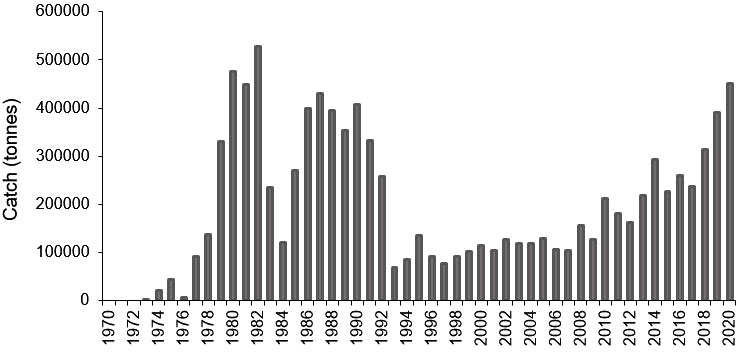
Figure 1 Antarctic krill catch 1970-2020 (CCAMLR, 2021).

The vast circumpolar distribution of krill (many potential habitats, Atkinson et al., 2008) and complex food–web relationships (Trathan and Hill, 2016; Warwick-Evans et al., 2021) are the obstacles to krill resource assessment. Krill are a micro-nektonic and move with ocean currents; they do have some behavioral control of their position in the water column (Nicol, 2006; Thorpe et al., 2007; Trathan et al., 2022). Therefore, the size, mobility, and variable behavior of krill are challenges for acoustic or net sampling (Watkins et al., 2016). On the other hand, estimating the krill standing stocks based on the acoustic data is restricted by limited spatial and temporal coverage (Reiss et al., 2008; Kinzey et al., 2015), particularly in near-shore waters (Trathan et al., 2022). Although a large number of investigations (Atkinson et al., 2017) and studies have been conducted on the assessment of Antarctica krill resources, estimates of their total biomass and production are still uncertain (Atkinson et al., 2009). In the Southern Ocean, due to the limitations of various factors, the large-scale scientific investigations had been undertaken only twice, one in 2000 (Watkins et al., 2004) and the other in 2019 (Krafft et al., 2021), which were both conducted in Area 48 of CCAMLR in the Atlantic sector, mostly stations concentrated in subareas 48.1–48.3 (Supplementary Figure 1).

Generally, the evaluations of distribution and biomass of marine organisms are based on scientific surveys characterized by the use of full-time dedicated vessels and pre-planned sampling designs (Gunderson, 1993). With the increased interest in acoustic data from fishing vessels, relative noise-mitigation (Wang et al., 2016), krill identification (Wang et al., 2017a), and statistical techniques for density estimation (Niklitschek and Skaret, 2016; Zhao et al., 2021) are already under development. The acoustic method to identify these swarms was established based on their biological characteristics using a biological swarm algorithm, which overcomes the limitations of having to use multiple frequencies in traditional frequency-difference identification methods (Wang et al., 2017a). This method improved the utility of fishing-vessel-based acoustic data for a range of objectives, and it was applied and validated based on the Antarctic krill resources data in the 2019 International Joint survey (Krafft et al., 2021). Multiple works using commercial fishing vessel acoustic data were promoted by the ASAM (SG-ASAM-2017, 2017; SG-ASAM-2018, 2018; SG-ASAM-2019, 2019); the outcomes indicated that fishery-based acoustic data could be applied to assess krill abundance. The methods using these acoustic data rationally and scientifically are being increasingly discussed (Watkins et al., 2016; Niklitschek and Skaret, 2016; Zhao et al., 2021).

Currently, to improve krill fishery monitoring and management, an important challenge is the estimation of krill population dynamics in the fishery hotspots (WG-EMM-2019, 2019; SC-CAMLR-XXXVIII, 2019). Thus, using fishery-based acoustic data in different spatiotemporal scales is useful to the assessment of krill density. However, the applications of the acoustic data collected during routine fishing operations remain in exploration (Watkins et al., 2016; Niklitschek and Skaret, 2016; Zhao et al., 2021), and there is no commonly used method. Though the spatial coverage of these trace tracking acoustic data is less systematically collected than the data in the general acoustic survey, these data cover more primary fishing grounds. At the same time, these data cover the entire fishing season, which can show the dynamic changes of krill density in fishing hotspots, and are of value to fishery management. Our objective is to develop a simple statistical approach to assess the density of Antarctic krill and an associated coefficient of variation (CV) using acoustic data collected by the krill fishing vessel from routine fishing operations.

Materials and methods

Fishing area

Surveys were conducted by the Chinese krill fishing vessel F/V Fu Rong Hai during the 2015/16 fishing season. The acoustic data were recorded using a scientific echosounder (Simrad EK60) at 38, 70, and 120 kHz. The acoustic navigation routes are depicted in Figure 2. Most fishing effort occurred in the Bransfield Strait, especially in a hotspot (59.50–57.75°W, 63.50–62.90°S) within the red polygon (Figure 2B). The bathymetry of the Bransfield Strait is generally shallower than 1000 m and characterized by steep slopes between the deep basin alongside the South Shetland Islands and Antarctic Peninsula. This topography with large depth gradient changes also complicates the physical environment of this region, especially the flow field (Wang et al., 2017a).

FIGURE 2

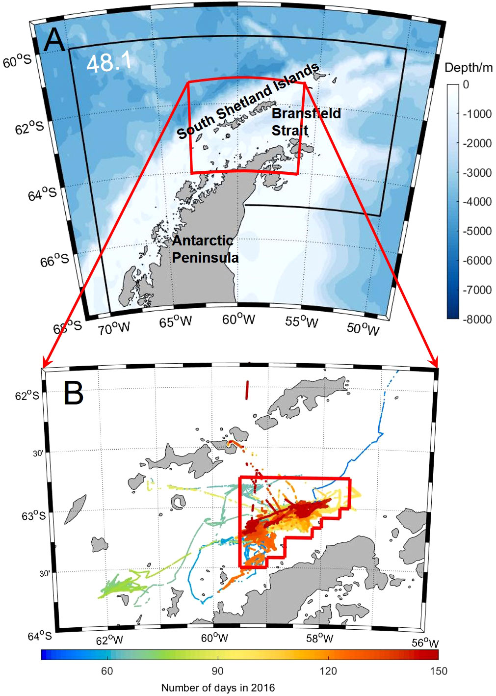
Figure 2 Study area: (A) CCAMLR Subarea 48.1 topography, (B): F/V Fu Rong Hai track lines, February–May 2016 (color intensity indicates number of days). The red polygon denotes area within grid 59.50–57.75°W, 63.50–62.90° S.

Acoustic data collection and processing

Acoustic data were collected using a Simrad EK60 echosounder system with hull-mounted transducers operating at 38, 70, and 120 kHz. Echosounder parameters were set in accordance with CCAMLR specifications (SC-CAMLR-XXX, 2011). Acoustic data were processed using Echoview (v 10.0.298). Krill backscatter was identified using a swarm-based method (Krafft et al., 2021) at 120 kHz, and a ‘nautical area scattering coefficient’ [acoustic density, NASC or S_A, m² nautical mile (nm)^-2] was integrated on a 0.1 nm horizontal resolution grid and exported for analysis. Detailed information of transducer specification and transceiver settings during data collection and the process of data analysis is described in Wang et al. (2017a).

Statistical approach

After the preprocessing of the raw data, the chaotic acoustic data were gridded, and the mean value for each grid was calculated to evaluate acoustic density. In the further processing involved, we assumed the distribution of krill population to be relatively random; then we averaged the data during a month as the monthly mean value, filtering the effect of tides on krill migration. The processed acoustic data had many zero and lower values with the horizontal resolution grid of 0.1 nm. We designed the Regional Gridding and Extended Delta-distribution model (hereinafter RGED model) to make reasonable use of these data to evaluate dynamic changes of krill density. This statistical method was verified by the data collected during the 2015/16 fishing season.

Regional gridding

According to the tracks of the fishing season vessel (to determine the study area boundary), we selected data from February–May 2016 from an area of ~1753 nm² (6013 km²) within the Bransfield Strait as our study area (Figure 2B). We designed 10 scenario simulations with different grid sizes. We divided the grid cells on the basis of the length along the meridian direction, respectively 1’S (about 1 nm), 2’S,…, 10’S, with the corresponding length along the latitude direction being 2’W, 4’W, …, 20’W, respectively. Within each grid cell, data were averaged for each month and treated as independent observations for that grid and that month.

A principle of grid size selection is that the coefficient of variation (CV) of acoustic density is relatively small, at the same time the proportion of effective covered area is relatively optimal. Accordingly, we design a selection index calculated as CV/weight of the effective covered area. The weight of the effective covered area is the proportion of the acoustic data coverage to the total study area. The smaller the selection index, the better the grid design. Additionally, we also refer to the common space between stations and data analysis methods for the design of fishing resource bottom trawl survey stations.

Extended delta-distribution model

Delta-distribution has been applied to the distribution of catch-per-tow data from trawl surveys for fish and plankton (Pennington, 1996; Pennington and Strømme, 1998; Li et al., 2008). The delta-distribution is a logarithmic normal distribution that includes data with a sample value of zero, and its non-zero value part is a logarithmic normal distribution, that is, the natural logarithm of non-zero value conforms to normal distribution. The statistical advantage of using the delta-distribution is that the estimator of the mean defined for this distribution is more efficient than the ordinary sample mean typically used to estimate abundance within study area strata (Smith, 1988). Smith and Pennington have conducted many studies on the application of this method in fisheries resource assessment (Smith, 1996; Pennington, 1983; 1986 and 1996). During the data analysis, density data (non-zero value part) are first converted to natural logarithm, with converted values then tested for goodness of fit to a normal distribution. The prerequisite for logarithmic transformation is that there can be no zeros in the sample. If they conform to a lognormal distribution, then the model is used for calculation.

Acoustic data are highly skewed to the right and usually have a cluster of smaller values relatively close to zero. Even after removing zero values, it is difficult to completely satisfy the normal/lognormal distribution. Myers and Pepin (1990) demonstrated that the sample mean and variance are more robust than lognormal-based estimators of mean and variance of population abundance if the data don’t follow a lognormal distribution. Because low values can severely bias lognormal-based estimators, we suppose the values greater than k are distributed approximately lognormally (Pennington, 1991; Kappenman, 1999). Here, k is a value to ensure that the values greater than it are approximately conforming to lognormal distribution. The basic principle of the method is as follows (Pennington, 1996; Folmer and Pennington, 2000).

Let ρ_i be the NASC value of Grid i (i∈n). An alternative estimator  ρ, as the mean of ρ_i is given by

$\begin{array}{ll}\rho =\frac{n-m}{n}\overline{y}+\frac{m}{n}\text{exp}\left(\overline{x}\right)g_m\left(\frac{s_x^2}{2}\right)& (1)\end{array}$

Where n is the number of sample values, m is the number of sample values > k, $\overline{y}$ denotes the mean of the value ≤ k, and $\overline{x}$ and $s_x^2$ are the mean and variance, respectively. Here x=ln(ρ_i)  of the logged values > k, g_m(t) is a function of m and t ( $t=\frac{s_x^2}{2}$) defined by

$\begin{array}{ll}{g}_m(t)=1+\frac{m-1}{m}t+{\sum }_{j=2}^{\infty }\frac{{(m-1)}^{2j-1}}{m^j(m+1)(m+3)\dots (m+2j-3)}·\frac{t^j}{j^{!}}& (2)\end{array}$

The estimator of the variance of ρ_i is given by

$\begin{array}{ll}\text{var}(\rho )=\text{var}({\rho }_x)+\left(\frac{n-m-1}{n(n-1)}\right)s_y^2+\left(\frac{m(n-m)}{n(n-1)}\right){\overline{y}}^2-2\left(\frac{n-m}{n(n-1)}\right)\overline{y}{\rho }_x& (3)\end{array}$

where $s_y^2$ is the variance of the values less than or equal to k, and ρ_x is the mean of the values greater than k,

$\begin{array}{ll}{\rho }_x=\frac{m}{n}exp(\overline{x})g_m\left(\frac{s_x^2}{2}\right)& (4)\end{array}$

and

$\begin{array}{ll}\text{var}({\rho }_x)=\frac{m}{n}\text{exp(}2\overline{x})\left\{\frac{m}{n}{g}_m^2\left(\frac{s_x^2}{2}\right)-\left(\frac{m-1}{n-1}\right)·g_m\left(\frac{m-2}{m-1}{s}_x^2\right)\right\} & (5)\end{array}$

The standard error (SE) of the mean density is estimated by

$\begin{array}{ll}\text{SE}(\rho )=\sqrt{\text{var}(\rho )}& (6)\end{array}$

An approximate 95% confidence interval for the mean density ρ is calculated as

$\begin{array}{ll}\rho \pm 1.96\text{SE}(\rho ) & (7)\end{array}$

The coefficient of variation (CV) is given as

$\begin{array}{ll}\text{CV}=\frac{\text{SE}(\rho )}{\rho }& (8)\end{array}$

When determining k, we use a Kolmogorov–Smirnov (K–S) test to determine if the non-zero part of the original data is subject to a normal or lognormal distribution. For our data, we consider the k value to be subject to a lognormal distribution.

Results

Sensitivity test of grid size

Using chaotic acoustic data during fishing operations from February 2016 as an example, the krill density scatter distributions in the study area in 10 different grid scenarios are illustrated in Figure 3. The scatter distributions in March–May 2016 are shown in the supplementary material (Supplementary Figures 2A–C). It can be seen that when the grid size is small, there are many zero and low values in the acoustic data, which is unsuitable for statistical analysis. With the increase of the grid size, the area covered by grid points accounts for a larger proportion of the total study area. The number of grid points and weights of effective areas within the research area in the 10 scenarios are presented in Figure 4.

FIGURE 3

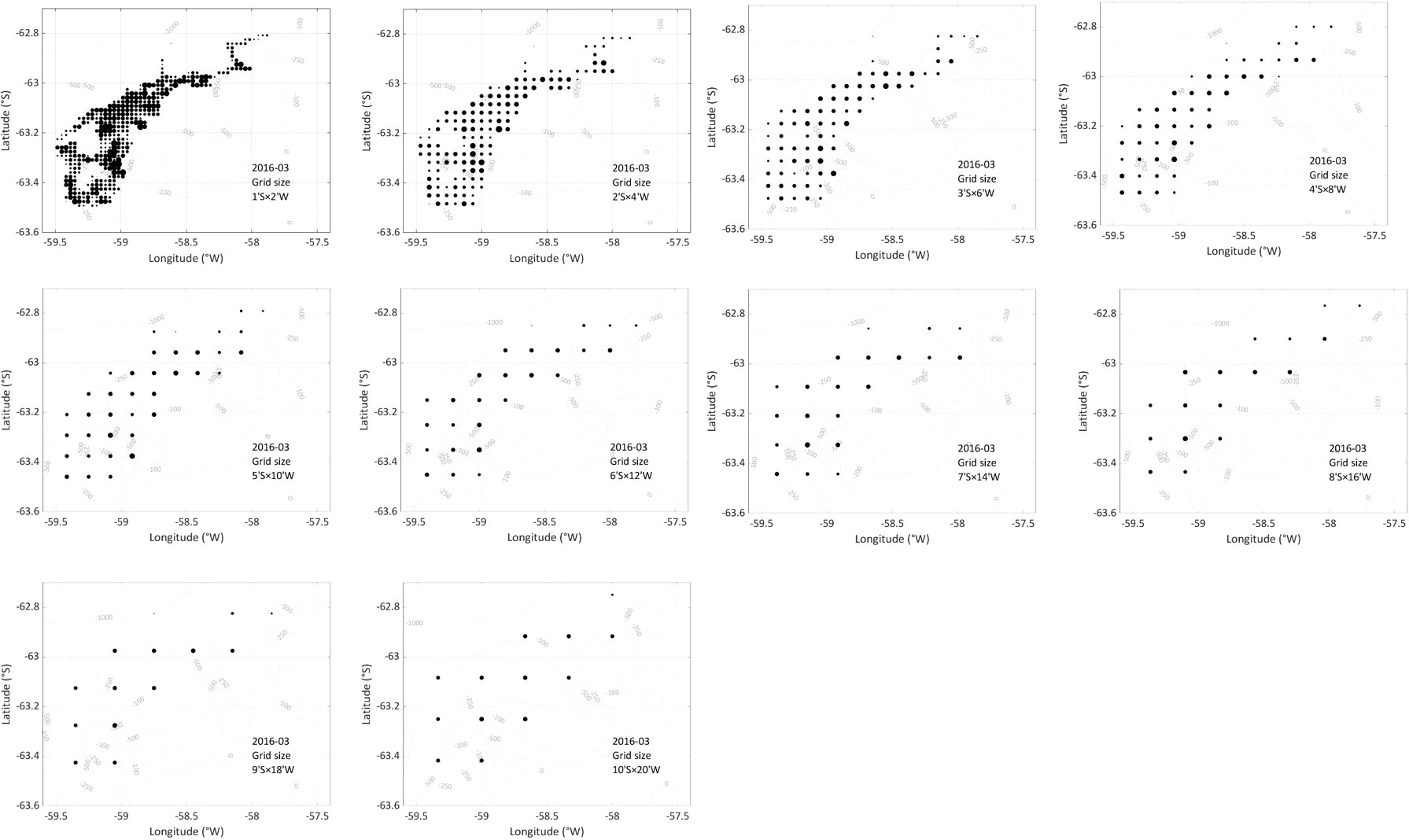
Figure 3 The scatter distributions of acoustic density for different grid sizes in February 2016. Circle diameter is proportional to krill density.

FIGURE 4

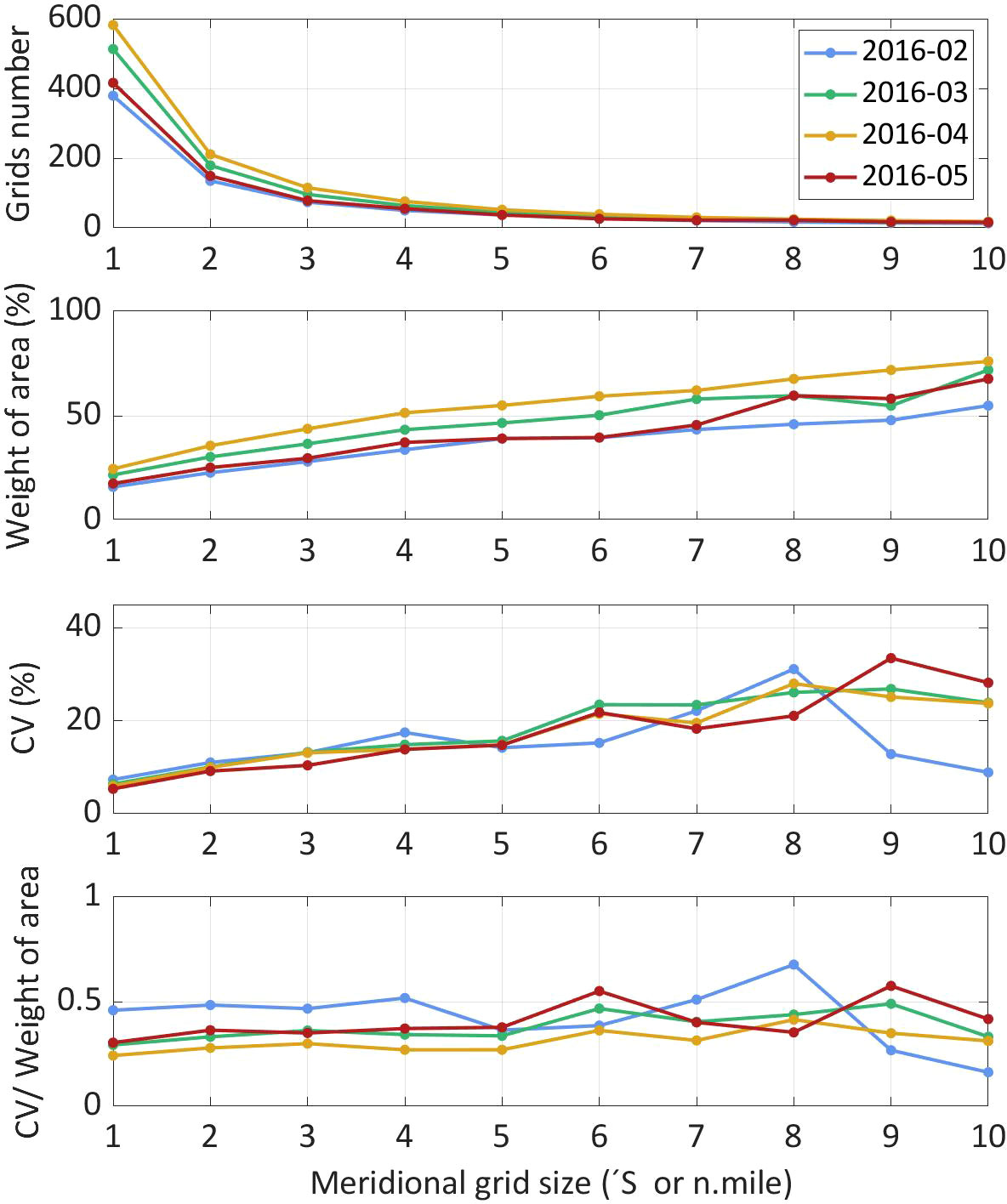
Figure 4 Gridded sample number, weight of effective covered area, coefficient of variation of the nautical area scattering coefficient (NASC), and grid selection index for different grid sizes.

Figure 4 also compares the CVs of the mean density for each scenario. When grid size decreased to<5 nm (meridian), CV values tended to converge. Few differences in CV were apparent among months at grid sizes<3 nm (meridian). At a grid size of 5′S × 10′W, the selection index (CV/Weight of effective covered area) decreased, with results for the four months being relatively homogeneous. In the survey designs of fishery resource assessment, a distance of 5 nm between stations is more commonly used. Accordingly, we selected the 5′S × 10′W grid to calculate krill resource density for this region.

Sensitivity test of the k value

The K-S test results of the extended delta-distribution model are shown in Table 1. After selecting the k value, the distribution of these data larger than the k value follows lognormal distribution and passes the hypothesis test of the significance level a = 0.05. Here the k value is the minimum value, and p-value >0.05 means the data obey a lognormal distribution. Histogram of the number of samples with a grid cell of 5′S × 10′W is shown in the supplementary material (Supplementary Figure 3).

TABLE 1

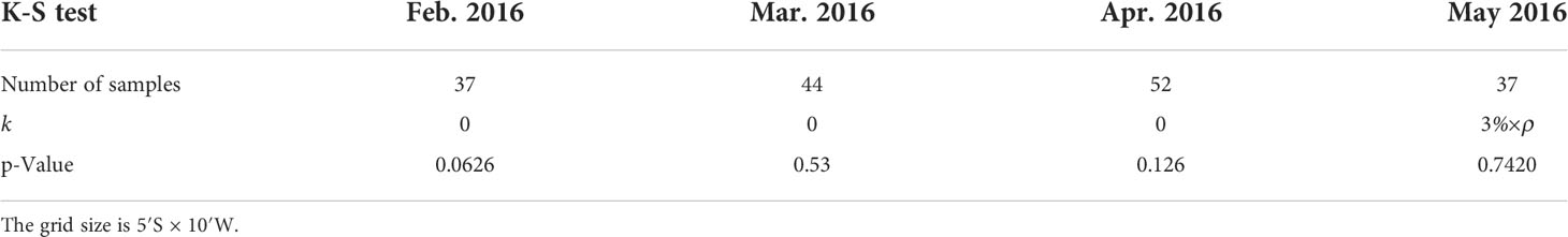
Table 1 From February to May 2016, the p-values corresponding to k values of the four groups of data and test values at the significance level a = 0.05 are shown in Table 1.

Krill density

Estimated krill density at multiple grid sizes (Figure 5) reveals similar means, but with some variation in confidence intervals among grid sizes, especially in high-density months (April and May). CVs generally increased with changing grid size (Figure 4). As grid size increased, the sample size used to estimate mean krill density decreased (Figure 3). Mean density was not strongly changing with grid size; however, a larger grid size resulted in greater variation (with larger confidence interval, CVs) in krill density estimates (Figure 5).

FIGURE 5

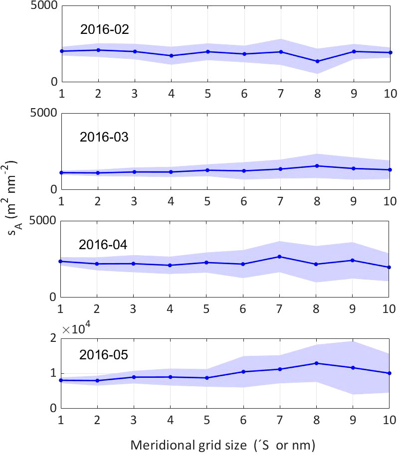
Figure 5 The estimations of nautical area scattering coefficient (NASC) in the hotspot with 10 gridding scenarios in February–May 2016. Error bars represent 95% confidence intervals of means.

The spatial distributions of acoustic density $S_A^{1/2}$ throughout the study area are presented in Figure 6, wherein differences in spatial sample sizes used to estimate pooled mean krill density of krill in fishery hotspots are apparent, with discrepant distribution in formations. Averaged acoustic density estimated in the hotspot with a 5’S × 10’W grid cell in February–May 2016 is presented in Figure 7 and Table 2. Krill density in the fishing ground is dynamic, and density was very high toward the end of the fishing season (May). Krill density in February was 1987.4 m² nm⁻² and reached 8757.9 m² nm⁻² in May (4.4× February values).

FIGURE 6

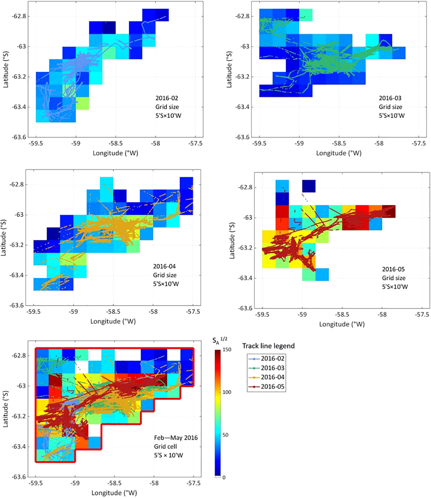
Figure 6 Monthly (February–May 2016) spatial distribution of nautical area scattering coefficient (NASC) values with a 5’S × 10’W grid cell.

FIGURE 7

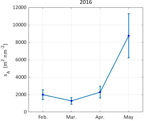
Figure 7 The estimations of the mean acoustic density in February–May 2016 in the fishing ground with a 5′S × 10′W grid cell. Error bars represent 95% confidence intervals of means.

TABLE 2

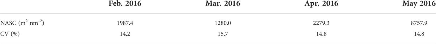
Table 2 Krill nautical area scattering coefficient (NASC) (= acoustic density), and coefficient of variation (CV) of the fishing ground in the Bransfield Strait in February–May 2016.

Discussion

Statistical approaches

The overall characteristics of acoustic data collected during fishing operations are disordered. As for traditional bottom trawl survey data, a proportion of zero or small values exist for sampling points (nets), and a proportion of sampling points have high density values. While traditional empirical statistical methods generally combine these zero, low, and high values, model-based methods generally treat them separately and, by doing so, better describe the resource distribution for an entire region (Gunderson, 1993; Li et al., 2008). According to the spatial distribution of krill acoustic density (Figure 6), the difference between high- and low-density areas is 10 or more times larger. Areas with high resource densities are inherent manifestations of the spatial distribution characteristics of fish populations, with high catch values making the distribution of resource density very discrete (Pennington, 1996). The working paper WG-FSA-2021/56 (Zhao et al., 2021) regarded high concentrations of, and high variation in, Antarctic krill resources to be natural characteristics of krill populations, for which reason the distribution of the Antarctic krill fishery must be highly concentrated, and the yield also highly variable.

Before using the extended delta-distribution model, we used the arithmetic average method, re-sampling (Bootstrap) method, delta-distribution model, and Gamma distribution models to perform relevant experimental simulations. Each approach has its pros and cons. When we use classical probability statistics in the study of data, data must be independent (random variables). However, the distribution of krill appears to have a degree of spatial correlation or continuity rather than being purely random. Here, we assume that the data is random and relatively independent. The mean density and CV calculated in our study using the arithmetic average method, Bootstrap method, and the extended delta-distribution model differed little (Supplementary Figure 4). On another side, if a data sample does not obey a normal distribution, the arithmetic mean method cannot accurately reflect the size characteristics of the variable, because this method is easily affected by the minimax value (Yuan et al., 2011). Taking this into account, the extended delta-distribution model in this paper has more advantages and stronger universality.

The delta-distribution model based on normal distribution has certain advantages over other methods in dealing with zero values (Smith, 1988; Pennington, 1996; Li et al., 2008). However, when processing acoustic data and simply using the delta-distribution model to analyze them, we find that non-zero data follow neither a normal nor logarithmic normal distribution, so CVs are large (Supplementary Figure 4). The extended delta-distribution model takes this problem into account.

The Gamma distribution model is not appropriate for analyzing samples with zero values (Smith, 1981). The average density and mean calculated using this model in monthly samples without zero values differ little from the extended delta-distribution model (Supplementary Figure 4). There is no zero value in the acoustic data of the 2015/16 fishing season applied, so the Gamma distribution model is applicable. However, if the data series has zero values, this method is not suitable (Supplementary Table 1).

The non-parametric Bootstrap method based on the resampling theory of EFRON (Efron, 1979) replicates observation information on the basis of the given original sample, does not need to make a distribution hypothesis or add new sample information, and can carry out statistical inference on the distribution characteristics of the whole population (Money and Duval, 1993; Zhao et al., 2010; Yuan et al., 2014). Although the spatial distribution of krill resources has not been determined, the Bootstrap method does not need to consider the overall distribution type. Therefore, this method can be used when there is uncertain data distribution, or the data layer distribution type is inconsistent (Zhao et al., 2021). The fitting analysis of the simulation results between the extended delta-distribution model and the bootstrap method showed high agreement, with R² = 0.9895 (Figure 8). In the case of this study, when the grid size is confirmed with 5′S × 10′W, the number of samples is around 37–52 (Table 1), so the two methods are both applicable (Supplementary Table 1). The bootstrap distribution is greatly affected by the samples; especially when the sample size is small, the bootstrap distribution will be significantly different. In this case, the bootstrap distribution reflects more the characteristics of the sample (Hesterberg et al., 2005). Therefore, with the increase of samples, the extended delta-distribution model might be more widely applicable.

FIGURE 8

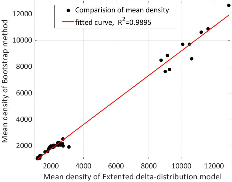
Figure 8 Fitting analysis of the simulation results (10 gridding scenarios) between extended the delta-distribution model and the bootstrap method.

Monthly variations of krill density

The Antarctic circumpolar current has a strong effect on the transportation of krill larvae, with the krill population distribution consistent with the overall current direction (Atkinson et al., 2008; Piñones et al., 2011; Piñones et al., 2013). For large-to-medium scale krill populations, ocean currents also influence their distribution, but how these currents retain or aggregate krill is not well understood (Reiss et al., 2008; Hinke et al., 2017). The Antarctic Ecosystem Research Division et al. (2016), indicated that seasonal horizontal migration of krill led to its accumulation in the Bransfield Strait, and the slower winter flow retained krill within it.

The krill hotspot that we report represents an important central fishing ground that for several months produces high yield (Ying et al., 2017; Wang et al., 2017b). Krill catch data statistics for this area reveals that with fishing season progression, krill fishery production sites gradually concentrated in the central Bransfield Strait, and by the end of summer and fishery closure, krill density in this hotspot trended significantly upward (Zhao et al., 2021). The direction of flow in the northern Bransfield Strait is from west to east, from the Bellingshausen Sea coastal current to the Bransfield Strait Current. The southern regional current forms a branch of the northward Antarctic coastal current from the Weddell Sea into the interior of the strait (Trathan et al., 2022). Currents from the Bellingshausen Sea and Weddell Sea intrude into the strait, providing a source of krill, and affecting changes in their biomass and biological structure. The special topography of the Bransfield Strait produces many eddies that provide an environment for the accumulation and retention of the krill. However, there are few reports detailing specific inputs and outputs of krill for this fishery hotspot. The driving mechanisms for the accumulation and retention of the krill in this hotspot need further research.

Krill fishery management

As krill is an important species in Antarctic marine ecosystems, the change of krill population will directly affect the entire ecosystem. Under the background of climate change, the health of the ecosystem has become a global concern. Striking a balance between conservation and sustainable fishery exploitation requires long-term monitoring and analysis of changes in the abundance and distribution of krill, which also presents a challenge for CCAMLR fisheries management (Wang et al., 2021). To promote the development of science-based management, the Commission endorsed a three-component strategy agreed upon by the Scientific Committee (CCAMLR-XXXVIII, 2019, para. 5.17; Ying et al., 2021): 1) the krill population is assessed to estimate a precautionary catch limit (i.e., the parameter gamma in the Generalized R Yield Model (GrYM) and the catch rate corresponding to a precautionary catch limit); 2) regular biomass estimate updates, initially at a subarea scale, but possibly at multiple scales; and 3) a risk-assessment framework to inform the spatial distribution of catches. It is not practical to regularly assess krill biomass by multi-year large-scale surveys. We explore how to apply acoustic data accumulated during routine commercial fishing operations to regionally assess krill density. Although this can only reflect the resource dynamic in the hotspot, it is a step towards achieving the goal of krill biomass assessment.

Conclusion

We present RGED model to process and apply “chaotic” acoustic data collected during routine fishing operations. Selection indexes calculated by the CV and weight of effective covered area of grids were screened using the Regional Gridding process. We then used an extended delta-distribution model to analyze the gridded data. Acoustic data collected by the Chinese krill fishing vessel F/V Fu Rong Hai since the 2015/16 fishing season in the Bransfield Strait were used as an application example. The results showed that the CV of the mean density for 4 months converged in a 5′S × 10′W grid cell at approximately 15%. Our method accurately reflects characteristics of the spatial and temporal distribution of krill density in the central Bransfield Strait fishing ground, with acoustic density in February of ~1990 m² nm^-2, reaching ~8760 m² nm^-2 in May. We demonstrate the RGED model to reasonably and scientifically analyze commercial fishery acoustic data collected during the production period to identify changes in Antarctic krill density and to provide a scientific basis upon which this fishery can be managed.

Data availability statement

The raw data supporting the conclusions of this article will be made available by the authors, without undue reservation.

Author contributions

YZ and XZ conceived the study. YZ led the study and writing of the manuscript. XW provided data and contributed substantially to writing the manuscript. YY contributed substantially to writing the manuscript. All authors read and approved the final manuscript.

Funding

This work was funded by the National Natural Science Foundation of China (No.42006194 and 41706219); the Marine S&T Fund of Shandong Province for Pilot National Laboratory for Marine Science and Technology (Qingdao) (No. 2022QNLM030002-1); the Major Scientific and Technological Innovation Project of Shandong Provincial Key Research and Development Program (No.2019JZZY010819); the Central Public-interest Scientific Institution Basal Research Fund, YSFRI, CAFS, China (No.20603022021017); and the Central Public-interest Scientific Institution Basal Research Fund, CAFS, China (No.2021TD02).

Acknowledgments

We would like to thank the fishing vessel F/V Fu Rong Hai for providing the acoustic data. We would also like to thank Steve O’Shea, PhD, from Liwen Bianji (Edanz) (www.liwenbianji.cn/), for editing the English text of a draft of this manuscript.

Conflict of interest

The authors declare that the research was conducted in the absence of any commercial or financial relationships that could be construed as a potential conflict of interest.

Publisher’s note

All claims expressed in this article are solely those of the authors and do not necessarily represent those of their affiliated organizations, or those of the publisher, the editors and the reviewers. Any product that may be evaluated in this article, or claim that may be made by its manufacturer, is not guaranteed or endorsed by the publisher.

Supplementary material

The Supplementary Material for this article can be found online at: https://www.frontiersin.org/articles/10.3389/fmars.2022.934504/full#supplementary-material

References

Antarctic Ecosystem Research Division, Southwest Fisheries Science Center and NOAA Fisheries, et al (2016). Background information to support development of a feedback management strategy for the krill fishery in subarea 48.1, WG-EMM-16/45. Hobart, Tasmania, Australia: CCAMLR.

Google Scholar

Atkinson A., Hill S., Pakhomov E. A., Siegel V., Anadon R., Chiba S., et al. (2017). KRILLBASE: a circumpolar database of Antarctic krill and salp numerical densitieS, 1926–2016. Earth System Science Data 9, 193–210. doi: 10.5194/essd-2016-52

CrossRef Full Text | Google Scholar

Atkinson A., Siegel V., Pakhomov E. A., Jessopp M. J., Loeb V. (2009). A re-appraisal of the total biomass and annual production of Antarctic krill. Deep-Sea Res. Part I: Oceanogr. Res. Papers 56 (5), 727–740. doi: 10.1016/j.dsr.2008.12.007

CrossRef Full Text | Google Scholar

Atkinson A., Siegel V., Pakhomov E. A., Rothery P., Loeb V., Ross R. M., et al. (2008). Oceanic circumpolar habitats of Antarctic krill. Mar. Ecol. Prog. Ser. 362, 1–23. doi: 10.3354/meps07498

CrossRef Full Text | Google Scholar

CCAMLR-XXXVIII (2019). Report of the thirty-eighth meeting of the commission (Hobart, Australia: CCAMLR).

Google Scholar

CCAMLR (2021). Statistical Bulletin (Hobart, Tasmania, Australia) Vol. 33. CCAMLR, Hobart, Tasmania, Australia. Available at: www.ccamlr.org.

Google Scholar

Efron B. (1979). Bootstrap methods: Another look at the jackknife. Ann. Statist. 7 (1), 1–26. doi: 10.1214/aos/1176344552

CrossRef Full Text | Google Scholar

Folmer O., Pennington M. (2000). A statistical evaluation of the design and precision of the shrimp trawl survey off West Greenland. Fish. Res. 49 (2), 165–178. doi: 10.1016/S0165-7836(00)00196-X

CrossRef Full Text | Google Scholar

Gunderson D. R. (1993). Surveys of fisheries resources (New York: Wiley).

Google Scholar

Hesterberg T., Moore D., Monaghan S., Clipson A., Epstein R. (2005). “Bootstrap methods and permutation tests,” in Introduction to the practice of statistics, 5th ed. New York: WH Freeman & Co.

Google Scholar

Hinke J. T., Cossio A. M., Goebel M. E., Reiss C. S., Trivelpiece W. Z., Watters G. M. (2017). Identifying risk: concurrent overlap of the Antarctic krill fishery with krill-dependent predators in the Scotia Sea. PloS One 12, e0170132. doi: 10.1371/journal.pone.0170132

PubMed Abstract | CrossRef Full Text | Google Scholar

Kappenman R. F. (1999). Trawl survey based abundance estimation using data sets with unusually large catches. ICES J. Mar. Sci. 56, 28–35. doi: 10.1006/jmsc.1998.0422

CrossRef Full Text | Google Scholar

Kinzey D., Watters G. M., Reiss C. S. (2015). Selectivity and two biomass measures in an age-based assessment of Antarctic krill (Euphausia superba). Fish. Res. 168, 72–84. doi: 10.1016/j.fishres.2015.03.023

CrossRef Full Text | Google Scholar

Krafft B. A., Macaulay G. J., Skaret G., Knutsen T., Bergstad O. A., Lowther A., et al. (2021). Standing stock of Antarctic krill (Euphausia superba Dana 1850) (Euphausiacea) in the Southwest Atlantic sector of the Southern Ocean 2018–19. J. Crustacean Biol. 41(3), 1–17. doi: 10.1093/jcbiol/ruab071

CrossRef Full Text | Google Scholar

Li F., Li X., Zhao X. (2008). Bottom trawl survey data analysis based on delta-distribution model and its application in the estimation of small yellow croak and silver pomfret in yellow Sea. J. Fish. China 32 (1), 145–151. (in Chinese, with English abstract). doi: 10.3321/j.issn:1000-0615.2008.01.023

CrossRef Full Text | Google Scholar

Money C. Z., Duval R. D. (1993). “Bootstrapping: A nonparametric approach to statistical inference,” in Sage university paper series on quantitative applications in the social sciences (Newbury Park: Sage).

Google Scholar

Murphy E. J., Watkins J. L., Trathan P. N., Reid K., Meredith M. P., Thorpe S. E., et al. (2007). Spatial and temporal operation of the Scotia Sea ecosystem: a review of large-scale links in a krill centered food web. Philos. Trans. R. Soc. B 362, 113–148. doi: 10.1098/rstb.2006.1957

CrossRef Full Text | Google Scholar

Myers R. A., Pepin P. (1990). The robustness of lognormal-based estimators of abundance. Biometrics 46, 1185–1192. doi: 10.2307/2532460

CrossRef Full Text | Google Scholar

Nicol S. (2006). Krill, currents, and sea ice: Euphausia superba and its changing environment. BioScience 56 (2), 111–120. doi: 10.1641/0006-3568(2006)056[0111:KCASIE]2.0.CO;2

CrossRef Full Text | Google Scholar

Niklitschek E. J., Skaret G. (2016). Distribution, density and relative abundance of Antarctic krill estimated by maximum likelihood geostatistics on acoustic data collected during commercial fishing operations. Fish. Res. 178, 114–121. doi: 10.1016/j.fishres.2015.09.017

CrossRef Full Text | Google Scholar

Pennington M. (1983). Efficient estimators of abundance, for fish and plankton surveys. Biometrics 39(1), 281–286.

Google Scholar

Pennington M. (1986). Some statistical techniques for estimating abundance indices from trawl surveys. Fish. Bull. 84, 519–525.

Google Scholar

Pennington M. (1991). Comments on the robustness of lognormal-based abundance estimators. Biometrics 47, 1623.

Google Scholar

Pennington M. (1996). Estimating the mean and variance from highly skewed marine data. Fish. Bull. 94, 498–505.

Google Scholar

Pennington M., Strømme T. (1998). Surveys as a research tool for managing dynamic stocks. Fish. Res. 37 (1-3), 97–106. doi: 10.1016/S0165-7836(98)00129-5

CrossRef Full Text | Google Scholar

Piñones A., Hofmann E. E., Daly K. L., Dinniman M. S., Klinck J. M. (2013). Modeling the remote and local connectivity of Antarctic krill populations along the western Antarctic peninsula. Mar. Ecol. Prog. Ser. 481, 69–92. doi: 10.3354/meps10256

CrossRef Full Text | Google Scholar

Piñones A., Hofmann E. E., Dinniman M. S., Klinck J. M. (2011). Lagrangian Simulation of transport pathways and residence times along the western Antarctic peninsula. Deep-Sea Res. Part II: Topical Stud. Oceanogr. 58 (13-16), 1524–1539. doi: 10.1016/j.dsr2.2010.07.001

CrossRef Full Text | Google Scholar

Reiss C. S., Cossio A. M., Loeb V., Demer D. A., et al (2008). Variations in the biomass of Antarctic krill (Euphausia superba) around the south Shetland islands 1996-2006. ICES J. Mar. Sci. 65 (4), 497–508. doi: 10.1093/icesjms/fsn033

CrossRef Full Text | Google Scholar

SC-CAMLR-XXX (2011). Report of the thirty-eighth meeting of scientific committee (Hobart, Australia: CCAMLR).

Google Scholar

SC-CAMLR-XXXVIII (2019). Report of the thirty-eighth meeting of scientific committee (Hobart, Australia: CCAMLR).

Google Scholar

SG-ASAM-2017 (2017). Report of the meeting of the subgroup on acoustic survey and analysis methods. In: Working Group meeting held in Qingdao, China (Hobart, Australia: CCAMLR).

Google Scholar

SG-ASAM-2018 (2018). Report of the meeting of the subgroup on acoustic survey and analysis methods. In: Working Group meeting held in Punta Arenas, Chile (Hobart, Australia: CCAMLR).

Google Scholar

SG-ASAM-2019 (2019). Report of the meeting of the subgroup on acoustic survey and analysis methods. In: Working Group meeting held in Bergen, Norway (Hobart, Australia: CCAMLR).

Google Scholar

Smith S. J. (1981). A comparison of estimators of location for skewed populations, with applications to groundfish trawl surveys. Can. Special Publ. Fish. Aquat. Sci. 58, 154–163.

Google Scholar

Smith S. J. (1988). Evaluating the efficiency of the Δ-distribution mean estimator. Biometrics 44 (2), 485–493. doi: 10.2307/2531861

CrossRef Full Text | Google Scholar

Smith S. J. (1996). Analysis of data from bottom trawl surveys. NAFO Sci. Council Stud. 28, 25–53. doi: 10.1016/S0967-0653(97)85798-5

CrossRef Full Text | Google Scholar

Thorpe S. E., Murphy E. J., Watkins J. L. (2007). Circumpolar connections between Antarctic krill (Euphausia superba dana) populations: investigating the roles of ocean and ice transport. Deep-Sea Res. Part I 54, 792–810. doi: 10.1016/j.dsr.2007.01.008

CrossRef Full Text | Google Scholar

Trathan P. N., Hill S. L. (2016). The importance of krill predation in the southern ocean. in: The biology and ecology of Antarctic krill, euphausia superba Dana 1850. Ed. Siegel V. (Dordrecht, The Netherlands: Springer), pp 321–pp 350.

Google Scholar

Trathan P. N., Warwick-Evans V., Young E. F., Friedlaender A., Kim J. H., Kokubun N. (2022). The ecosystem approach to management of the Antarctic krill fishery - the “devils are in the detail” at small spatial and temporal scales. J. Mar. Syst. 225, 103598. doi: 10.1016/j.jmarsys.2021.103598

CrossRef Full Text | Google Scholar

Wang X. L., Skaret G., Godø O. R. (2017a). Processing of acoustic recordings from krill fishing vessels collected during fishing operations and surveying. In: Working Paper submitted to the CCAMLR Working Group on Acoustic Survey and Analysis Methods (SG-ASAM-2017/03). (Hobart, Australia: CCAMLR). Available from the CCAMLR Secretariat or the authors.

Google Scholar

Wang X. L., Skaret G., Godø O. R., Zhao X. Y. (2017b). Dynamics of Antarctic krill in the bransfield strait during austral summer and autumn investigated using acoustic data from a fishing vessel. In: Working Paper submitted to the CCAMLR Working Group on Ecosystem Monitoring and management (WG-EMM-2017/40) (Hobart, Australia: CCAMLR). Available from the CCAMLR Secretariat or the authors.

Google Scholar

Wang X. L., Zhang J. C., Zhao X. Y. (2016). A post-processing method to remove interference noise from acoustic data collected from Antarctic krill fishing vessels. CCAMLR Sci. 23, 17–30.

Google Scholar

Wang X. L., Zhao Y. X., Fan G. Z., Ying Y. P., Zhao X. Y., Zhang J. C. (2021). Acoustic biomass estimates of Antarctic krill in subarea 48.1 to facilitate the development of the new management approach for the krill fishery. In: Working Paper submitted to the SC-CAMLR (SC-CAMLR-2021/13). CCAMLR, Hobart, Australia. Available from the CCAMLR Secretariat or the authors.

Google Scholar

Wang X. L., Zhao X. Y., Zou B., Fan G. Z., Yu X. T., Zhu J. C., et al. (2019). Implementation and preliminary results from the synoptic krill survey in Area 48, 2019 conducted by the Chinese krill fishing vessel Fu Rong Hai. In: Working Paper submitted to the CCAMLR Working Group on Ecosystem Monitoring and management (WG-EMM-2019/43). CCAMLR: Hobart, Australia. Available from the CCAMLR Secretariat or the authors.

Google Scholar

Warwick-Evans V. A., Santora J., Waggitt J. J., Trathan P. N. (2021). Multi-scale assessment of distribution and density of procellariiform seabirds within the Northern Antarctic Peninsula marine ecosystem. ICES Journal of Marine Science. doi: 10.1093/icesjms/fsab020

PubMed Abstract | CrossRef Full Text | Google Scholar

Watkins J. L., Hewitt R., Naganobu M., Sushin V.. (2004). The CCAMLR 2000 survey: a multinational, multi-ship biological oceanography survey of the Atlantic sector of the southern ocean. Deep Sea Res. Part II Topical Stud. Oceanogr. 51, 1205–1213. doi: 10.1016/S0967-0645(04)00075-X

CrossRef Full Text | Google Scholar

Watkins J. L., Reid K., Ramm D., Zhao X. Y., Cox M., Skaret G., et al. (2016). The use of fishing vessels to provide acoustic data on the distribution and abundance of Antarctic krill and other pelagic species. Fish. Res. 178, , 93–,100. doi: 10.1016/j.fishres.2015.07.013

CrossRef Full Text | Google Scholar

WG-EMM-2019 (2019). Report of the Meeting of the Working Group on Ecosystem Monitoring and Management. In: Working Group meeting held in Concarneau, France (Hobart, Australia: CCAMLR).

Google Scholar

Ying Y. P., Wang X. L., Zhu J. C., Zhao X. Y. (2017). Krill CPUE standardisation and comparison with acoustic data based on data collected from Chinese fishing vessels in subarea 48.1. In: Working Paper submitted to the CCAMLR Working Group on Ecosystem Monitoring and management (WG-EMM-2017/41) (Hobart, Australia: CCAMLR).

Google Scholar

Ying Y. P., Zhao X. Y., Fan G. Z., Wang X. L. (2021). The various spatial scales available for consideration and the distribution of the krill fishery in Subarea 48.1. In: Working Paper submitted to the CCAMLR Working Group on Acoustic Survey and Analysis Methods (WG-ASAM-2021/09). CCAMLR, Hobart, Australia. Available from the CCAMLR Secretariat or the authors.

Google Scholar

Yuan X. W., Jiang Y. Z., Cheng J. H. (2011). Estimating the average stock density with dominating large catches based on Δ–distribution model. Prog. Fish. Sci. 32 (1), 1–7 (in Chinese, with English abstract). doi: 10.3969/j.issn.1000-7075.2011.01.001

CrossRef Full Text | Google Scholar

Yuan X. W., Yan L. P., Liu Z. L., Cheng J. H. (2014). A performance comparison of stock density estimation of Larimichthys polyactis in the East China Sea using different models based on bottom trawl survey. South China Fish. Sci. 10 (6), 20–26 (in Chinese, with English abstract). doi: 10.3969/j.issn.2095-0780.2014.06.003

CrossRef Full Text | Google Scholar

Zhao L., Chen J. X., Xu M. Q., Li M. (2010). Bootstrap method and its application in biology. J. Zool. 29 (4), 638–641 (in Chinese, with English abstract). doi: CNKI:SUN:SCDW.0.2010-04-045

Google Scholar

Zhao X. Y., Wang X. L., Ying Y. P., Fan G. Z., Xu Q. C., Gao D. Q., et al. (2021). The potential impact of krill fishery concentration needs to be assessed against the highly patchy and dynamic nature of krill distribution. In: Working Paper submitted to the CCAMLR Working Group on Fish Stock Assessment (WG- FSA-2021/56). Hobart, Australia: CCAMLR. Available from the CCAMLR Secretariat or the authors.

Google Scholar

Zhao Y. X., Wang X. L., Zhao X. Y., Ying Y. P., Zhang J. C. (2021). Monthly variation of Antarctic krill biomass in a main fishing ground in the Bransfield strait based on fishing vessel acoustic data collected during routine fishing operations. In: Working Paper submitted to the CCAMLR Working Group on Acoustic Survey and Analysis Methods (WG-ASAM-2021/10). Hobart, Australia: CCAMLR. Available from the CCAMLR Secretariat or the authors.

Google Scholar

Zhao X. Y., Zuo T., Leng K. L., Tang Q. S. (2016). Engineering science and technology challenges in the Antarctic krill fishery. Chinese Journal of Engineering Science. 18, 2, 85–90 (in Chinese, with English abstract). doi: 10.15302/J-SSCAE-2016.02.010

CrossRef Full Text | Google Scholar